Abstract

Patients with Type I Diabetes (T1D) must take insulin injections to prevent the serious long term effects of hyperglycemia – high blood glucose (BG). These patients must also be careful not to inject too much insulin because this could induce hypoglycemia (low BG), which can potentially be fatal. Patients therefore follow a “regimen” that, based on various measures, determines how much insulin to inject at certain times. Current methods for managing this disease require adjusting the patient’s regimen over time based on the disease’s behavior (recorded in the patient’s diabetes diary).

If we can accurately predict a patient’s future BG values from his/her current features (e.g., predicting today’s lunch BG value given today’s diabetes diary entry for breakfast, including insulin injections, and perhaps earlier entries), then it is relatively easy to produce an effective regimen. This study explores the challenges of BG modeling by applying a number of machine learning algorithms, as well as various data preprocessing variations (corresponding to 312 [learner, preprocessed-dataset] combinations), to a new T1D dataset that contains 29 601 entries from 47 different patients. Our most accurate predictor is a weighted ensemble of two Gaussian Process Regression models, which achieved an $err_{L1}$ loss of $2.70$ mmol/L (48.65 mg/dl). This was an unexpectedly poor result given that one can obtain an $err_{L1}$ of $2.91$ mmol/L (52.43 mg/dl) using the naive approach of simply predicting the patient’s average BG. For each of data variant and model combination we report several evaluation metrics, including glucose-specific metrics, and find similarly disappointing results – again, the best model was only incrementally better than the simplest measure. These results suggest that the diabetes diary data that is typically collected may not be sufficient to produce accurate BG prediction models; additional data may be necessary to build accurate BG prediction models.

1 Introduction

Individuals suffering from Type I diabetes (T1D) are unable to produce insulin, meaning their bodies cannot properly regulate their blood glucose (BG) [1] – i.e., cannot maintain their BG between 4 – 8 mmol/L [2]. As a result, T1D is a serious long term condition that can lead to microvascular, macrovascular, neurolgical and metabolic complications [1, 2].

To manage their diabetes, patients give themselves periodic injections of insulin as directed by their health care team. Injecting too much insulin may induce hypoglycemia (BG$<4$ mmol/L, in our study), which can be dangerous, possibly causing a coma. However, injecting too little insulin can result in hyperglycemia (BG$>8$ mmol/L, in our study), which may lead to chronic complications such as blindness, kidney failure, nerve damage and circulatory problems [1, 2]. In general, a patient’s BG will depend on many factors, including past carbohydrate intake, the amount of bolus/basal insulin injected, exercise, and stress [2].

Diabetes patients try to properly maintain their BG in a normal range. This is challenging because tight glycemic control using bolus insulin injections (whether intermittent with insulin pens or boluses using insulin pumps) is associated with an increased the risk of having hypoglycemic events [1]. This challenge has led to attempts to create closed-loop systems and the use of computational techniques that assist in controlling patient’s BG levels [3]. An extreme example of this is the effort to create an “artificial pancreas”, which explicitly integrates automatic monitoring with automatic administration of insulin [4].

Another perspective on fully automated diabetes management views the BG control problem as two sequential subproblems:

1. “modeling”: learning an accurate BG prediction model that, for example, predicts the BG level at lunch given a description of the subject throughout breakfast (including perhaps her previous BG values, carbohydrate intake, etc., from earlier meals), as well as the amount of insulin injected at breakfast.

2. “controlling”: given the current information (at breakfast), consider the effects of injecting various possible amounts of insulin – e.g., {1 unit, 1.5 units, 2 units, …}. For each, use the learned model to predict the BG value at lunch, then inject the amount that is predicted to lead to the best lunch time BG-value (Of course, this assumes that decisions made at breakfast only affect lunch, then lunch decisions will only affect dinner, etc. – which does not consider the longer-range effects of actions; see Bastani [3]).

This paper focuses on the first subtask: developing a BG prediction system, where in general, a model $M$ will predict the blood glucose $\widehat{\hbox{{\sc BG}}_{i+1}}\ =\ M(\,x_{i},\,\Delta t_{i+1}\,)$ at the next time point ($\Delta t_{i+1}$ minutes into the future), based on information currently known about this patient, including the amount of insulin (bolus_i) the patient decided to inject (Note that this abstracts some issues; see Appendix A.1 for details):

$$x_{i}\quad=\quad[\hbox{{\sc time}${}_{i}$, \ {\sc BG}${}_{i}$,\ {\sc bolus}${}_{i}$,\ {\sc basal}${}_{i}$,\ {\sc EV}${}_{i}$,\ {\sc PV}${}_{i}$,\ {\sc IOB}${}_{i}$,\ \ldots}]$$ (1)

An example of this subtask might be to predict an individuals blood glucose at 12:01pm lunch on Tuesday, given information collected up-until 8am breakfast on Tuesday(Where this could only include the Tuesday breakfast information, or it could include other earlier information – e.g., the ellipses in Equation 1 might contain information about events from yesterday, or last week).

Explicitly, the goal of this work is to to determine if it is possible to accurately predict a T1D patient’s recorded BG, from one meal to the next, based only on the information typically recorded by the patient. To do this, a model must be able to deal with the data provided in a patient’s diabetes diary, which has varied prediction horizons.

This work is an extensive effort to learn an accurate BG prediction model, which involved exploring 312 different combinations of learner and preprocessing variant. To train and evaluate each of these variants, we used a dataset of 29 601 entries collected from 47 unique patients, where each entry included the information typically collected, including: the time of day, the patient’s current BG, the carbohydrate about to be consumed and the anticipated exercise.

1.1 Background Literature and its Limitations

As the mechanism of diabetes are not completely understood, we are considering the machine learning approach of learning a model, from a large labeled dataset, containing many records from many Type-1 diabetes patients. Of course, this requires access to such a dataset. Previous studies have been based on data from small numbers of subjects and/or data collected over a short time period. For example, several studies have been based on data from a single patient where records were only collected for fewer than 100 days [5, 2, 6, 7]. These studies are limited because different patients behave very differently. Other studies include more patients (12 – 15) but only have 3 – 22 days worth of data [8, 9]. Another study used three patients with two years of data [10]. Further, studies analyzing continuous glucose monitoring (CGM) data from larger patient sets (89 T1D patients) exist but are again sampled over relatively short periods of time (1 week) [11]. In these last four cases, datasets either had short histories for their patients or they had a small number of patients in total. In contrast, our work uses a larger number of patients who had up to two years worth of data, where records were collected multiple times each day.

There are large datasets of type-2 diabetes patients – e.g., Quinn et al. [12] measured glycated hemogloben changes in data collected data from 163 patients over the course of a year. However, studies that model type-2 diabetes [13, 14] should not be directly compared to those that model type-1 diabetes because there are significant differences between these diabetes types. In particular, there is less variance in the blood glucose readings over time for type-2 patients than there is for type-1 patients, making type-2 patients easier to model.

While we focus on predicting BG values many hours later, some studies instead attempt to predict the occurrence of hypoglycemic events, and only within a short window (e.g., 30 to 120 minutes) [15, 16, 8, 17, 18]. Indeed, a literature review by Contreras et al. identified 49 publications using modeling techniques for blood glucose prediction (primarily with T1D patients) of which 38 used predictions horizons that were 60 minutes or less [19]. Of these, one of these publications included prediction horizons of 180 minuets but on simulated data, and another had 1440 minute prediction horizons but used a dataset of 8 patients collected over only 3 days [19]. While this might help to protect patients from a very serious situation, it is lacking in several ways. First, such fine-grained measurements are often not practically obtainable outside of a study setting and without using a CGM device that provides measurements every 5 minutes. Second, these short-term predictions are not adequate for spanning the time between meals. Third, the goal of building a diabetes control system is better served with a more expressive model, as opposed to one that can only provide binary classifications – hypoglycemic or not. Note that these model provides no useful feedback for situations where patients are hyperglycemic.

In our work, we try to model blood glucose dynamics (including both hyperglycemia and hypoglycemia) and using only the standard records collected at meal times. While this makes our task more challenging, we do this because it involves only the data that medical professionals most often encounter in practice.

Like Pappada et al. [20], we also considered neural network models. After training on 17 T1D patients, Pappada et al.’s [20] evaluation, on a single held-out patient, yielded “scores” (a version of the rL1 measure defined in Equation 5) of 0.067 (resp., 0.089, 0.117, 0.145, 0.166, 0.189) when using predictive windows of 50 (resp., 75, 100, 120, 150 and 180) minutes in the future. While they were able to achieve a score of 0.189 using 180 minute predictive windows, note that their result is based on the test data of a single patient (other patients may be more difficult to predict) and that the dataset used in their study involved relatively short-range predictions (50 – 180 minutes), while our study involves predictions made, on average, 310.6 minutes in the future (averaging 593 minutes for overnight predictions and 236 minutes otherwise). Since Pappada et al. showed that larger predictive windows decrease the accuracy of their models, we expect that our data should be more difficult to model well. Also, their study involved only 3 to 9 days of data with continuous glucose monitoring, whereas our data were collected over a period of months to years.

Our work resembles previous works [21, 22] that use Gaussian Process Regression (GPR) for modeling diabetes. In particular, Duke [22] used GPR to learn models of individual patients that could be used to aid in cross-patient prediction. We similarly explore some transfer learning techniques with GPR, along with ensembles of learners and various other machine learning algorithms.

Prior works have also addressed the blood glucose modeling problem that we explore in this work [2, 6, 7]. These latter two evaluate their results using normalized blood glucose values; since they are unitless normalized values, they cannot be directly interpreted in terms of mmol/L, which means that we cannot compare our results to theirs. However, we do evaluate the performance of a model that is similar to the Gaussian Wavelet Neural Network used in the third [7].

One work of interest to our study is the previously mentioned 2018 publication by Gadaleta et al. [11] that analyzes CGM data. In comparison to our work, this work looks at shorter term blood glucose predictions over a shorter period of time but is similar in that it provides a fairly comprehensive analysis of the predictive performance of many different machine learning models. Gadaleta et al. focus on two different methods for training and evaluating models, “static” and “dynamic”. Similarly to their “dynamic” training process, the majority of our study focuses on training and testing on data from each patient separately. However, the stacking models used in our work effectively train a “static” model with a Leave One Patient Out and combine this model with a patient-specific model. Gadaleta et al. consider combining “static” and “dynamic” training processes as future work.

There are other works that define measures for evaluating the quality of glucose predictors, in general. In particular, Del Favero et al. [23] describes several different measures for comparing a patient’s specific glucose reading, with a predicted one, including both standard measures (like L1, relative L1 error, and L2 losses – there called MAD, MARD and RMSE) and some “glucose-specific metrics”, such as gMAD and gRMSE [24]. While our paper focuses on the L1 and relative L1 errors, we also include the others mentioned there.

1.2 Main Contributions

Below we list the main contributions of this work:

1. To our knowledge, this study examines the largest multi-year dataset of diabetes diary records, collected from Type 1 diabetes patients, used for modeling future BG.

2. We provide a comprehensive study of this data, considering 312 combinations of learning algorithm and type of data, to determine if machine learning can be used to create an accurate blood glucose prediction model.

3. Our results demonstrate that it is difficult for a machine learned model to perform better than a naive baseline (in this case, predicting a patient’s average BG), when considering both standard error measures, like L1 and L2 loss, and also for glucose-specific measures, such as gMAD.

The publically available MSc thesis [25] that corresponds to this work provides additional information, including a breakdown of the individual patients in the study, more detailed results, and a comparison to a diabetologist’s performance on this prediction task.

2 Materials and Methods

Section 2.1 first summarizes how we obtained this (real world) data; Section 2.2 then describes the pre-processing steps required to make this data usable. We then consider two ways to modify this dataset: Section 2.3 considers modifying the set of records; one class of studies involves the complete set of entries, and another class included just the subset of “Expert Predictable” records (defined below). For each of these two “sets of record”, we consider various “feature sets” – the original set of features, and also 12 other variants, each of which includes various new features, that are combination of those original features; see Section 2.4. Section 2.5 then summarizes the 12 different learning algorithms we considered (based on 7 distinct base learners); and Section 2.6.1 describes a trivial baseline, to help us determine whether the results of any of the learned models are actually meaningful. This requires describing how we evaluate the quality of a learned model – see Section 2.6. (This segues naturally to Section 3, which provides those empirical results.)

2.1 Dataset

This study used 47 patient histories from Type I diabetes patients, which were collected using the “Intelligent Diabetes Management” (IDM) software(described in Ryan et al. [26]). Note that the associated website https://idm.ualberta.ca/ has since been decommissioned. This data included patients who participated in Ryan et al.’s study, as well as additional patients who began using the IDM software after the completion of the study (up until December 2016). The participants gave their informed written consent, and the Research Ethics Board of the University of Alberta approved the collection and analysis of the data. For further details regarding patient participation, see Ryan et al. [26]. Some of the participants only used the system a few times. As we wanted to focus on patients that had sufficient information to find relevant patterns, we only included patients who made at least 100 diabetes diary entries with the system – i.e., produced at least 100 “sufficient” records. This led to a dataset of 16 pump users and 31 non-pump patients. Table 1 provides summary statistics for our data. The dataset used for this work differs from the one described in Borle [25] in that we limit the number of patients included to those with complete data.

Patient #16 is noteworthy for having by far the most records of any patient in our dataset; it is unusual for a patient to consistently produce diabetes entries over the course of many years. Because of the large number of records, we use part of this patient’s dataset as our hyper-parameter tuning (validation) dataset, as well as for visualization.

Table 1: Summary of Demographics

Distinct Patients	Age	Height	Weight	Sex	Pump Users
47	$42\pm 13$	$166\pm 8$ cm*	$74\pm 14$ kg	47 (9 $\mars$ / 38 $\venus$)	16

* Height could not be obtained for 7 individuals, so this average value was calculated using only the remaining patients. See Borle [25] for more details about individual patients.

Each record $i$ corresponds to an entry in a patient’s “diabetes diary”, which includes the meal associated with the record meal_i, a time stamp (date_i and time_i), the blood glucose value BG_i, the grams of carbohydrates consumed CHO_i, and the units of bolus (resp., basal) injected bolus_i, (resp., basal_i). The patients also entered the anticipated level of exercise using the non-numeric values {“less than normal”, “normal”, “active”, “very active”}. We converted these into numeric values ($2$, $4$, $7$ and $10$ respectively) for use by standard learning algorithms.

As was mentioned, 16 of the patients in this study used insulin pumps, which each directly infuse insulin from a reservoir, via a catheter, just under a patient’s skin at a basal rate. Moreover, they also self-inject larger amounts of bolus insulin when a patient ingests carbohydrates (as a patient would with an insulin pen http://www.diabetes.org/living-with-diabetes/treatment-and-care/medication/insulin/how-do-insulin-pumps-work.html). Each record of each insulin pump patient includes the basal infusion rate value PV_i, in $\frac{units}{hour}$. The insulin pump settings work by partitioning the 24h clock into intervals, and setting a particular delivery rate of insulin for each interval. The PV_i values for any specific record was then set to the insulin delivery rate for the interval containing the record’s time stamp We also computed two other features: $\Delta t_{i}$, which is the elapsed time since the previous record (Actually, $\Delta t_{i}$ is based on previous bolus_i-1 and CHO_i-1 values; see Appendix A.1) and “Insulin on Board” IOB_i, which captures the effect of any insulin remaining in a person’s system from previous injections [27]. This was based on the following pairs of elapsed time and percentage of post-injection insulin remaining [28]: (1.66 hours, 78%), (2.5 hours, 48%), (3.33 hours, 27%), (4.15 hours, 12%), (5 hours, 3%). We then used a simple spline to interpolate these values; see Fig 1. Table 2 formalizes all of these features and Table 3 provides example data.

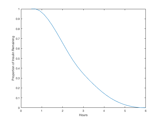
Fig 1: Spline of Insulin on Board over Time.

2.2 Data Preprocessing

The first step in analyzing the data was dealing with the missing or erroneous (unreasonably low) values. We discarded any record that did not have an associated BG value (572 records). This was necessary as we cannot evaluate a model on records where we do not have a ground truth for BG. We also discarded any records that had missing dates (6 records) because these timestamps are integral to deriving features from the data. Second, we changed any BG value less than 1 mmol/L (8 records) to 1 mmol/L, as glucose meters are simply not accurate at these low values, other than to state that the values are very low. We then log-transformed these blood glucose values for all our predictors, anticipating that this log-linear model would have better performance. This means that after this model makes a prediction, we must use simple exponentiation to transform that prediction back into the original interpretable units.

To address missing bolus insulin and CHO carbohydrate values, we imputed average values into the missing entry (variants for this step are described in Section 2.4). This was done on a per-subject, per-meal basis – that is, we imputed an individual’s average value for a particular meal. For example, say a specific patient injected, on average, 3 units of bolus insulin before breakfast. Whenever she does not enter the before-breakfast insulin, we replace that missing value with “3 units”. When dealing with missing exercise values, we imputed the “normal” value. For missing basal insulin values, we always imputed a constant value of 0. This allows a learner to distinguish when basal insulin was recorded and when it was not. After this preprocessing, we computed the auxiliary features ($\Delta t_{i}$, IOB_i) from the improved data. We describe the complete set of features in Table 6, and we show example records as columns in Table 7; see also Appendix A.1.

Table 2: Description of Original Features, and some Computed Features, used in this Study

meali	The time of day: { Before Breakfast, After Breakfast, Before lunch, After Lunch, Before Supper, After Supper, Before Bed, During the Night}
datei	The date as year-month-day
timei	The time as hour:minute:second
BGi	The BG value at the current time ($\frac{mmol}{L}$)
CHOi	The amount of carbohydrates ingested (grams)
bolusi	The amount of insulin injected (units)
basali	The units of background insulin injected
EVi	Numeric encoding of exercise value: $\{2,4,7,10\}$
PVi	Pump Value: The rate at which the insulin pump is infusing ($\frac{units}{hour}$). This is always 0 if the patient does not have a pump.
$\Delta t_{i}$	The elapsed time since last record
IOBi	Insulin on Board: Estimated residual insulin from the previous injection ($\frac{mmol}{L}$)

See text for further description of these terms. Note this is a simplified set of features; see Table 6 in the Appendix for the complete set of feature descriptions.

Table 3: Example of Data, over a single day, from Patient 16

index $i$	27	28	29	30	31	32
meali	Before Breakfast	After Breakfast	Before Lunch	After Lunch	Before Dinner	After Dinner
datei	2015-11-25	2015-11-25	2015-11-25	2015-11-25	2015-11-25	2015-11-25
timei	08:36:00	10:19:00	12:19:00	15:35:00	18:42:00	20:11:00
BGi	16.2	14.7	5.6	6.8	10.5	3.0
CHOi	30.0	0	30.0	0	15.0	0
bolusi	10.4	0	3.0	0	3.8	0
basali	0	0	0	0	0	0
EVi	4	4	4	4	4	4
PVi	0.50	0.50	0.63	0.45	0.90	0.90
$\Delta t_{i}$	540	103	120	196	187	89
IOBi	0.00	7.90	3.61	0.89	0.81	3.35

Note this is a simplified version of the data; Table 7 in the Appendix provides the general, complete set of features.

2.3 Subset of only “Expert Predictable” Entries

As our data was collected voluntarily from patients at their own convenience, sampling intervals are not uniform, and the relevant data is not recorded for every meal. This is problematic for our predictive task as blood glucose values are more difficult to predict as more time elapses between readings. To address this issue, our clinician co-author (E.A.R.) established the following criteria of when it is reasonable to predict the next glucose value; the BG is “expert predictable” (EP) at a given time if all of the following are true:

1. The preceding record is not a hypoglycemic event ( Note that this is difficult to predict due to potential glucose counterregulation effects [29] and the uncertainty in BG that follows from a physiological response to hypoglycemia).

2. The blood glucose reading is present for the preceding meal. For example, to make a prediction about a patient’s blood glucose value before lunch, a record detailing his/her previous breakfast must be available.

3. Six of the last eight days prior to a prediction must have records for both the current meal time and the previous meal time. For example, to predict the blood glucose before lunch, six of the last eight days must have both “before lunch” and “after breakfast” entries, to help capture this “after breakfast to before lunch” transition pattern.

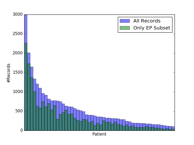
Fig 2: Records Meeting the EP Criteria From Section 2.3. Patients are sorted by descending total numbers of records. See Borle [25] for further details.

Fig 2 shows the number of records from each patient that qualify as EP – the number of records for which our expert would feel comfortable making predictions.

Later, we trained and evaluated 13 models using the entire dataset $D$ (called { $D_{a}$1, $D_{a}$2, …, $D_{a}$13}) as well as 13 corresponding models that were trained and then evaluated, using only the records that met the expert’s EP criteria, $D^{EP}$ (called { $D_{e}$1, $D_{e}$2, …, $D_{e}$13 }). Note that the $D_{a}$ and $D_{e}$ notation reflects that a dataset was derived from either all the data points ($D_{a}$) or from the expert’s subset $D^{EP}$ ($D_{e}$).

2.4 Feature Engineering

Table 2 shows the basic features used to describe each event. Additionally, we also considered many other feature sets to see if any could lead to better performance. Some of the variants completed records that were missing entries for carbohydrates or bolus insulin, which others removed those deficit records. Some added in the day of the week as an integer feature or as a one-hot encoded feature (http://scikit-learn.org/stable/modules/generated/sklearn.preprocessing.OneHotEncoder.html), while others removed the “basal insulin” feature. A few variants included non-temporal patient characteristics: age, gender, height and weight. Some replaced the set of features with just the first 4 principal components (obtained by principal component analysis, PCA).

Our “Kok Features” variant uses computed features similar to Kok [2], and subsequently used by Baghdadi et al. [6] and Zainuddin et al. [7]. Unlike Kok’s data, however, we do not have stress level values in our data and were therefore unable to incorporate that feature.

For any given dataset variant, some models have components that train on different subsets of the data. In addition, we also use models that include components that are trained on the data from all patients other than the current test patient, as well as models that involve sub-models that are each trained only on data from one meal type (e.g., before breakfast).

Note we consider each of these variants applied to the original dataset, and also to the reduced “EP-filters” datasets; see Section 2.3. Note that this reduces the predictions that our system attempts. For example, we do not attempt to predict a before-lunch BG value if there is no preceding after-breakfast reading. For each variant, we only considered the subset of the records that belonged to that variant, both for producing the model and also for estimating the quality of that model – in particular, the thirteen “EP”-models were trained and tested on the $D^{EP}$ set of records.

Table 8 (in Appendix A.1) describes all our dataset variants.

2.5 Machine Learning Algorithms

This work considers twelve different learners, based on seven base learning algorithms, each run on each of the various different datasets (differing based on the feature preprocessing used; see Section 2.4 K-Nearest Neighbors (KNN), Support Vector Regression (SVR), Artificial Neural Networks (ANN), Wavelet Neural Networks (WNN), Ridge Regression (RR), Random Forest Regression (RFR) and Gaussian Process Regression (GPR). We used patient#16’s first 3260 diabetes diary entries from dataset D21 to tune the hyper-parameters for the different base learners – e.g., for the GPR model (nugget = 0.25), KNN model (K = 10, weighting = uniform), RF model (maximum depth = 4), and our neural network model (batch size = 20, epochs = 1000). These 3260 records were then excluded from our testing data to reduce the risk of overfitting. All other unspecified parameters were defaults – e.g., the linear SVR model (C = 1), SVR with RBF kernel model (C = 1, $\sigma^{2}=\frac{1}{\hbox{\# of features}}$) and Ridge regression model ($\alpha$ = 1) are the defaults provided by scikit-learn [30]. The ANN architecture included one output neuron with linear activation and two hidden layers of $3\times(\hbox{\# of features})$ with rectified linear activation. The WNN architecture included one output neuron with linear activation and one hidden layer of $(\hbox{\# of features})$ neurons with Gaussian wavelet activations ($\Psi(x)=-xe^{-\frac{1}{2}x^{2}}$). Most of these models were implemented with the help of scikit-learn [30], except for the ANN that was implemented using Keras [31] and the WNN that was implemented in part with scikit-neuralnetwork
(http://scikit-neuralnetwork.readthedocs.io/en/latest/index.html). We assume the reader is familiar with these fairly standard learners.

We also combined base learners to develop more complex learners. The following section (Section 2.5.1) describes our GPR ensemble approach. We also considered another approach, which incorporates the information from the other patients – e.g., use patient histories #1 to #46 to help train a model for patient #47. This “Stacking” approach first trains a model on the auxiliary patients, then runs this model on the test patient’s data to produce a new feature for each meal – i.e., a 14th feature, to augment the 13 features shown in Table 7. Appendix A.6 shows the entire stacking process.

2.5.1 Modeling with a confidence weighted GPR Ensemble, $M_{gpr}^{w}$

For each patient, our “GPR ensemble” model first creates two different GPR models, then combines them into a single model called $M^{w}_{gpr}$. The first of these two models, $GPR_{p}$, learns from the entirety of a patient’s training data. The second model, $\{GRP_{m}\}$, is actually a collection of GPR models – one for each possible meal category $m$ (corresponding to meal_i in Table 2. Each of these $GPR_{m}$ models is trained using only the occurrences of that particular meal category in the patient’s training data (e.g., all occurrences of “Before Lunch”). Once we have obtained $GPR_{p}$ and the set of $GRP_{m}$ models and wish to make a prediction for instance $x_{i}$, we produce a weighted prediction of the form

$$\widehat{BG_{i+1}}\quad=\quad\frac{1}{\alpha+\beta}\left[\alpha\ GPR_{p}(\,[x_{i},\Delta t_{i+1}]\,)\ +\ \beta\ GPR_{m}(\,[x_{i},\Delta t_{i+1}]\,)\ \right]$$ (2)

where $\alpha=\frac{1}{{\sigma_{p}}_{i}}$ and $\beta=\frac{1}{{\sigma_{m}}_{i}}$, and where ${\sigma_{p}}_{i}$ and ${\sigma_{m}}_{i}$ are respectively the standard deviations of the posterior Gaussian distributions $\mathcal{N}(\,GPR_{p}(\,[x_{i},\Delta t_{i+1}]\,),\,{\sigma^{2}_{p}}_{i}\,)$ and $\mathcal{N}(\,GPR_{m}(\,[x_{i},\Delta t_{i+1}]\,),\,{\sigma^{2}_{m}}_{i}\,)$ at the point $x_{i}$.

2.6 Model Evaluation

To assess the performance of our models in general, evaluation functions are required to measure the quality of model predictions with respect to known true outcomes. In this paper we report our results in terms of “$L_{1}$-loss” ($err_{L1}$), “relative $L_{1}$-loss” ($err_{rLl}$) and Root Mean Squared Error (RMSE).

Given a model $M(\cdot)$ and a dataset

$$D\quad=\quad\{\,[\,[x_{i},\Delta t_{i+1}],\ \hbox{{\sc BG}}_{i+1}\,]\,\}_{i}$$ (3)

where each $x_{i}$ provides the “temporal information” shown in Equation 1, “$L_{1}$-loss” ($err_{L1}$), “relative $L_{1}$-loss” ($err_{rLl}$), and RMSE are defined as

$$\hbox{err}_{L1}(\,M(\cdot),D\,) = \frac{1}{|D|-1}\sum_{i=1}^{|D|-1}|\ M(x_{i},\,\Delta t_{i+1})-\hbox{{\sc BG}}_{i+1}\ |$$ (4)

$$\hbox{err}_{rL1}(\,M(\cdot),D\,) = \frac{1}{|D|-1}\sum_{i=1}^{|D|-1}\frac{|\ M(x_{i},\,\Delta t_{i+1})-\hbox{{\sc BG}}_{i+1}\ |}{\hbox{{\sc BG}}_{i+1}}$$ (5)

$$RMSE({M(\cdot),D}) = \sqrt{\frac{1}{|D|-1}\sum_{i=1}^{|D|-1}(\ M(x_{i},\,\Delta t_{i+1})-\hbox{{\sc BG}}_{i+1}\ )^{2}}$$ (6)

where BG_i+1 is the blood glucose associated with the next time point, occurring $\Delta t_{i+1}$ minutes later (Note that Del Favero et al. [23] refers to $err_{L1}$ and $err_{rLl}$ as MAD and MARD, respectively).

For each of these three metrics we also consider “glucose-specific” variants. These “glucose-specific” variants use a “Clark Error Grid inspired penalty function” to re-weight the relative costs of different mispredictions (see Del Favero et al. [23] for descriptions and definitions). Therefore in total, we consider the performance of our models across 6 different evaluation functions (See Appendix A.3 for why we include both $err_{L1}$ and $err_{rLl}$).

2.6.1 Baseline: Using a Naive Predictor

To establish a baseline for evaluating these learned models, we created a naive model ($M_{avg}$) that, for each patient, simply predicted that patient’s average BG value (over all meals/records) based on his/her diabetes history – that is, the naive model predicted the same average value (for that patient), independent of any other information about that patient. More concretely, given a patient’s data $D=\{[\dots,BG_{i},\dots]\}_{i}$, partitioned into a training set $D^{train}$ and a test set $D^{test}$, the model calculates the average blood glucose for the entire training set

$$BG_{avg}(D^{train})\quad=\quad\frac{1}{|D^{train}|}\sum_{[\dots,BG_{i},\dots]\in D^{train}}BG_{i}$$ (7)

including readings for all meals and all days. Then for all instances $x_{j}$ in the associated test set $D^{test}$, this model sets $M_{avg}(\,x_{j},\,\Delta t_{j+1}\,)\ =\ BG_{avg}(D^{train})$. So, for patient $16$: as the BG_avg value for her first training set was 8.4, this trivial model predicts that her blood glucose value will be 8.4 for each meal in the associated test set. We can then evaluate this trivial model using Equations 4,  5 and  6; we clearly hope that the less-trivial models will do significantly better.

2.6.2 10-Fold Cross Validation

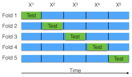
Fig 3: Illustration of 5-Fold CV with Contiguous Segments. In each CV iteration training is done on the blue segments and testing on the green segment.

Each of our learners will take the entire dataset and produce a model. The next challenge is evaluating this learned model. To evaluate the predictive quality of each learner, we use 10-fold cross validation (CV), with respect to each patient. We first partition time series history of a patient, denoted $X_{i}$, into ten contiguous segments $X_{i}=\bigcup_{j=1..10}X_{i}^{j}$. We then use nine of the ten segments for training in each CV round and use the remaining one segment for testing – so the first split would be train $X^{1}_{i,tr}=\bigcup_{j=2..10}X_{i}^{j}$ and test $X^{1}_{i,te}=X_{i}^{1}$. While the testing partition always consists of contiguous data, the training partition will not always be completely contiguous. Fig 3 provides a visualization of what it means to partition time series data into contiguous segments for the purposes of cross validation – for simplicity, here we show “5-fold CV” rather than 10.

3 Results

3.1 Cross Validation Results

In this section we will discuss the results of our models when evaluated with cross validation on the dataset variants created. Again, 12 different learners were evaluated (derived from 7 base learners) and 26 different dataset variants ($D_{e}$1 through $D_{e}$13, and $D_{a}$1 through $D_{a}$13) were created for the purpose of this analysis. For each of the 47 patient histories not used for hyperparameter selection (described in Section 2.1), we perform 10-fold CV using $12\times 26$ different learner/dataset-variant combinations to determine their effectiveness and how well they compare to the baseline model, $M_{ave}$ from Section 2.6.1. Appendix A.2 provides details about the models, and Appendix A.4 provides heat-maps that show both the performance of models on different datasets (in terms of $err_{L1}$ and $err_{rLl}$), as well as the improved performance relative to $M_{ave}$. Appendix A.5 also shows the performance of these learned models in terms of other measures.

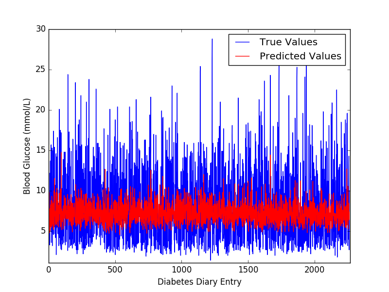
Fig 4: Model $M^{w}_{gpr}$: Our GPR ensemble’s predictions on data from patient 16.

For each learner and dataset variant pair, we compute the $err_{L1}$ error as a micro-average over all the records of each patient. These results allow us to determine the pair with the lowest average $err_{L1}$, over all 47 patient histories: These studies found that $M^{w}_{gpr}$ had the lowest $err_{L1}$ on average across all of the 26 different preprocessing variants of the data. On dataset $D_{e}$1 (the preprocessing variant with the lowest average $err_{L1}$ across all models), $M_{ave}$’s average $err_{L1}$ was 2.91 mmol/L, while $M^{w}_{gpr}$’s average $err_{L1}$ was 2.70 mmol/L – i.e., our best model saw an improvement of only 7.1% relative to the baseline!

To help understand why the improvement is not greater, Fig 4 shows the predictions of $M^{w}_{gpr}$ for the processed entries from patient#16 that were used for selecting hyperparameters. Here, we can see that the model is unable to account for the high amount of variance present in the BG records for this patient.

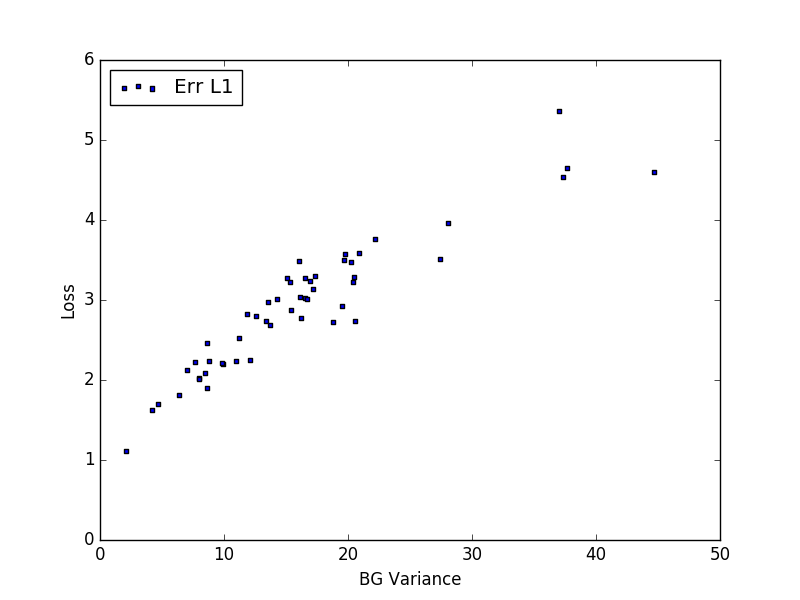
Fig 5: Model $M^{w}_{gpr}$: average $err_{L1}$ as a function of BG variance, for all patient histories.

Fig 5 plots the variance in each patient’s BG history and the corresponding patient’s $err_{L1}$ loss (Equations 4) that $M^{w}_{gpr}$ was able to achieve. This figure shows that the variance of a patient’s blood glucose was highly correlated with the $err_{L1}$ test loss ($0.93$ Pearson Correlation).

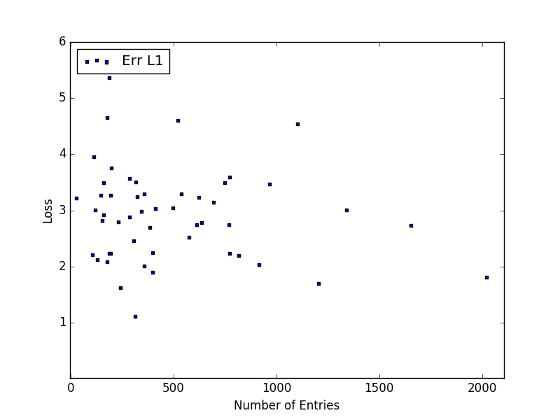
Fig 6: Model $M^{w}_{gpr}$: average $err_{L1}$ as a function of the # of diabetes diary entries for a patient, for all patient histories.

Fig 6 is a scatter plot of $err_{L1}$ loss as a function of the number of data points that were available for each patient in the dataset. This figure suggests that there is no relationship between how well the model performs (in terms of $err_{L1}$ test loss) on any particular patient, and how many data points were collected from that patient – Pearson Correlation: -$0.14$.

3.2 Other Evaluation Measures

We then considered the $err_{rLl}$ loss and found that $M^{w}_{gpr}$’s $err_{rLl}$ loss on $D_{e}$1 was 0.361. We also saw that $M^{w}_{gpr}$ achieved the best $err_{rLl}$, although this was on a different dataset-variant. The best [model, dataset-variant] pair was $M^{w}_{gpr}$ on dataset $D_{e}$11, which achieved an average $err_{rLl}$ error of 0.348; this was an improvement of 19.0% relative to the $M_{avg}$ baseline of 0.430. Note that $M^{w}_{gpr}$ achieved an $err_{L1}$ of 2.78 mmol/L dataset $D_{e}$11.

In addition to our $err_{L1}$ and $err_{rLl}$ metrics we also report RMSE and the glucose-specific versions of these metrics in Table 5. Interesting the best model across all metrics was $M^{w}_{gpr}$, and the best dataset preprocessing variant was either $D_{e}$1 or $D_{e}$11 (both $D_{e}$ variants).

Table 4: Performance of the best models across all metrics on $D_{e}$ Datasets.

Metric	Naive Model Error	Best Model Error	Percent Improvement	Best Model	Best Dataset Variant
RMSE	3.58	3.47	2.98%	$M^{w}_{gpr}$	$D_{e}$1
$err_{L1}$ (MAD)	2.91	2.70	7.12%	$M^{w}_{gpr}$	$D_{e}$1
$err_{rLl}$ (MARD)	0.430	0.348	18.97%	$M^{w}_{gpr}$	$D_{e}$11
gRMSE	5.01	4.86	2.95%	$M^{w}_{gpr}$	$D_{e}$1
gMAD	5.31	4.98	6.28%	$M^{w}_{gpr}$	$D_{e}$1
gMARD	0.783	0.648	17.28%	$M^{w}_{gpr}$	$D_{e}$11

Note that these error values are micro-averages. These are selected entries from the tables in Supporting Information Section A.5.

Table 5: Performance of the best models across all metrics on $D_{a}$ Datasets.

Metric	Naive Model Error	Best Model Error	Percent Improvement	Best Model	Best Dataset Variant
RMSE	3.67	3.58	2.49%	$M^{w}_{gpr}$	$D_{a}$1
$err_{L1}$ (MAD)	2.96	2.78	6.14%	$M^{w}_{gpr}$	$D_{a}$1
$err_{rLl}$ (MARD)	0.422	0.355	15.88%	$M^{w}_{gpr}$	$D_{a}$11
gRMSE	5.16	5.02	2.70%	$M^{w}_{gpr}$	$D_{a}$1
gMAD	5.45	5.14	5.70%	$M^{w}_{gpr}$	$D_{a}$1
gMARD	0.772	0.660	14.50%	$M^{w}_{gpr}$	$D_{a}$11

Note that these error values are micro-averages. These are selected entries from the tables in Supporting Information Section A.5.

4 Discussion

Our results show that our best learning algorithm is more accurate than a naive baseline – but only slightly – and that it can only achieve an average $err_{L1}$-loss of approximately 2.70 mmol/L. This loss means that, on average, if the patient’s blood glucose was normal (e.g., 6 mmol/L), the learned model may incorrectly identify the patient as either hypoglycemic (as $6-2.70<4$ mmol/L) or hyperglycemic ($6+2.70>8$ mmol/L). Together with the strong relationship between glucose variance and prediction error, this highlights how challenging it is to create models that produce fine-grained blood glucose predictions when only using diabetes diary entries – i.e., using only the information that is commonly available to medical practitioners.

Having tried 312 different combinations of learners and dataset variants, and observing minimal differences in their performance, it seems unlikely that another [learner, dataset-variant] combination would be better. Note that these limited results include models that use data from multiple patients, which suggest that simply including more patients in the study is not likely to improve model performance. Moreover, since the model accuracy did not seem to improve as the number of recorded entries increased, we suspect that simply collecting more of these entries for each individual will not improve model performance.

There are many possible reasons why modeling T1D glucose levels based on this standard type of diabetes diary data is so challenging. It is possibly just an artifact of our study: perhaps many of the patients who volunteered, did so because their diabetes was difficult to manage. Another reason could be that inaccuracies and omissions of variables in data prevent the model from producing accurate predictions. These omissions could possibly include: not knowing the site where the bolus insulin was injected, how much scar tissue was present at the injection site, skin temperature, how accurately the carbohydrate value was recorded, the accuracy of the recorded insulin dose, the levels of different hormones, whether the patient was menstruating, stress levels, accuracy of recording exertion, insulin age or storage conditions, amount of blood flow at the injection site and likely yet other factors. Given our belief that training more accurate models will require additional relevant variables, future research might incorporate more confounding variables, such as injection location [32], glucagon levels [33] and/or meal protein/fat content [34]. However, it is not clear which, if any, of such variables are sufficient to explain the response, nor whether they can be practically captured in a clinical setting.

5 Conclusion

This work explored the challenge of accurately predicting future blood glucose values in Type I diabetes patients, based on various models learning using several machine learning algorithms. Our extensive explorations – involving 12 different learning algorithms, and 26 different encodings of the data (312 combinations) – found that, on average, the model with the lowest expected $err_{L1}$ was a confidence weighted Gaussian process regression model ($M^{w}_{gpr}$). Using 10-fold cross validation on 29 601 blood glucose records from 47 different patients, our $M^{w}_{gpr}$ model performed only $7.1\%$ better than the naïve “mean predicting” model ($M_{avg}$). Anecdotally, a diabetologist also attempted to do this task – predicting the BG for the next meal. We found that this model’s predictions (insignificantly) outperformed the diabetologist’s, in terms of a simple unbiased loss function, but that the diabetologist performed (insignificantly) better when the evaluation was biased toward predicting hypoglycemic events; see Borle [25].

These results showed that our model could achieve an expected absolute error of $2.70$ mmol/L (48.65 mg/dl), which is disconcertingly large given that this is based on the type of data that is frequently collected and used for clinical practice (records are collected at meal times by the patients themselves). These results strongly suggest that the standard data collected by T1D patients, while apparently appropriate for clinical treatment of T1D, is not sufficient for accurately predicting blood glucose levels. We conjecture that using patient data that is sampled more frequently and that includes additional features would improve both the ability of professionals and machine learning practitioners to more accurately predict patient’s blood glucose levels, but there is a practical trade-off between patient convenience and highly detailed record keeping.

Appendix A Supporting Information

A.1 Dataset Preprocessing Variants and Example

As mentioned earlier, the features that we described in Section 2.2 are simplified so that they can be easily understood. This appendix describes the complete set of features that we used.

The previously described $\Delta t_{i}$ and BG_i features implicitly assume that the previous event involved both injecting a quantity of insulin and also consuming some carbohydrates. While this is typically the case, there are exceptions. To accommodate such situations, where an event involves only one of these, we decompose each of these terms into two different features: $\Delta t_{i}$ is separated into $\Delta t^{bolus}_{i}$ and $\Delta t^{CHO}_{i}$, and BG_i is separated into BG_i^bolus and BG_i^CHO. These correspond to the time since most recent (previous) bolus injection $\Delta t^{bolus}_{i}$ (when bolus_i- bolus units were injected and the blood glucose was BG_i^bolus), and the time since the most recent previous carbohydrate consumption $\Delta t^{CHO}_{i}$ (when the subject consumed CHO_i- and his/her blood glucose was BG_i^CHO).

Table 6 provides the complete set of features that we used and Table 7 provides the correct version of Patient#16’s data from Table 3 with these features.

Table 6: Description of Original and Processed Features used in this Study

meali	The time of day: { Before Breakfast, After Breakfast, Before lunch, After Lunch, Before Supper, After Supper, Before Bed, During the Night}
DOWi	The day of the week
xVi	Numeric encoding of exercise value: $\{2,4,7,10\}$
PVi	Pump Value: The rate at which the insulin pump is infusing ($\frac{units}{hour}$). This is always 0 if the patient does not have a pump
basali	The units of background insulin injected
BGi	The BG value at the current time ($\frac{mmol}{L}$)
IOBi	Insulin on Board: Estimated residual insulin from the previous injection ($\frac{mmol}{L}$)
CHOi-	The previous most recent amount of carbohydrates ingested (grams)
bolusi-	The previous most recent amount of insulin injected (units)
BGi-CHO	The BG value at the time that CHOi- was ingested ($\frac{mmol}{L}$)
BGi-bolus	The BG value at the time that bolusi- was injected ($\frac{mmol}{L}$)
$\Delta t^{CHO}_{i}$	The time between CHOi- and BGi+1 (min)
$\Delta t^{bolus}_{i}$	The time between bolusi-and BGi+1 (min)

Table 7: Example of Processed Data, over a single day, from Patient 16 (Variant D1)

index $i$	27	28	29	30	31	32
meali	Before Breakfast	After Breakfast	Before Lunch	After Lunch	Before Dinner	After Dinner
DOWi	Tuesday	Tuesday	Tuesday	Tuesday	Tuesday	Tuesday
EVi	4	4	4	4	4	4
PVi	0.50	0.50	0.63	0.45	0.90	0.90
basali	0	0	0	0	0	0
BGi	16.2	14.7	5.6	6.8	10.5	3.0
IOBi	0.00	7.90	3.61	0.89	0.81	3.35
CHOi-	17.5	30.0	20.5	30.0	18.5	15.0
bolusi-	1.93	10.40	2.44	3.00	2.54	3.80
BGi-CHO	10.3	16.2	14.7	5.6	6.8	10.5
BGi-bolus	10.3	16.2	14.7	5.6	6.8	10.5
$\Delta t^{CHO}_{i}$	540	103	120	196	187	89
$\Delta t^{bolus}_{i}$	540	103	120	196	187	89

Note that $\hbox{{\sc BG}}_{i}^{CHO}$ will differ from $\hbox{{\sc BG}}_{i}^{bolus}$ and $\Delta t^{CHO}_{i}$ will differ from $\Delta t^{bolus}_{i}$whenever carbohydrates and insulin were not taken at the same time.

Table 8 lists all of the dataset variants that are generated by the various feature-creation/selection steps. Note the first 13 datasets ($D_{e}$1 - $D_{e}$13) contain only the subset of records that satisfy the EP criteria – see Section 2.3. The second 13 rows ($D_{a}$1 - $D_{a}$13) deal with, essentially, the entire set of records. The “Missing Carbs” and “Missing Bolus” columns address variants in handling missing data, “PCA Transformation” indicates if the features were transformed using PCA, the “Kok features” column indicates datasets that use the features described by Peter Kok and the remaining columns indicate whether specific other features are included.

Table 8: Datasets Generated from Different Feature Sets.

	# of Subjects	Records Predicted	EP Rules	DOW Features	Basal Feature	Patient Specific Features	Kok Features	PCA Transform	Missing Carbs	Missing Bolus
$D_{e}$1	42	7378	1	1	1	0	0	0	Throwout	Impute Mean
$D_{e}$2	39	5978	1	1	1	0	0	0	Throwout	Throwout
$D_{e}$3	47	16167	1	1	1	0	0	0	Impute Mean	Impute 0
$D_{e}$4	47	16167	1	1	1	0	0	0	Impute 0	Impute Mean
$D_{e}$5	47	16167	1	7	1	1	0	0	Impute Mean	Impute Mean
$D_{e}$6	47	16167	1	1	1	0	0	0	Impute Mean	Impute Mean
$D_{e}$7	47	16167	1	7	1	0	0	0	Impute Mean	Impute Mean
$D_{e}$8	47	16167	1	0	0	0	0	0	Impute Mean	Impute Mean
$D_{e}$9	37	7349	1	0	0	0	1	0	N/A	N/A
$D_{e}$10	47	16167	1	1	1	0	0	0	Impute 0	Impute 0
$D_{e}$11	45	10623	1	1	1	0	0	0	Impute Mean	Throwout
$D_{e}$12	47	16167	1	0	0	0	0	1	Impute Mean	Impute Mean
$D_{e}$13	37	7349	1	0	0	0	1	1	N/A	N/A
$D_{a}$1	42	15961	0	1	1	0	0	0	Throwout	Impute Mean
$D_{a}$2	39	13832	0	1	1	0	0	0	Throwout	Throwout
$D_{a}$3	47	24896	0	1	1	0	0	0	Impute Mean	Impute 0
$D_{a}$4	47	24896	0	1	1	0	0	0	Impute 0	Impute Mean
$D_{a}$5	47	24896	0	7	1	1	0	0	Impute Mean	Impute Mean
$D_{a}$6	47	24896	0	1	1	0	0	0	Impute Mean	Impute Mean
$D_{a}$7	47	24896	0	7	1	0	0	0	Impute Mean	Impute Mean
$D_{a}$8	47	24896	0	0	0	0	0	0	Impute Mean	Impute Mean
$D_{a}$9	37	11888	0	0	0	0	1	0	N/A	N/A
$D_{a}$10	47	24896	0	1	1	0	0	0	Impute 0	Impute 0
$D_{a}$11	45	19122	0	1	1	0	0	0	Impute Mean	Throwout
$D_{a}$12	47	24896	0	0	0	0	0	1	Impute Mean	Impute Mean
$D_{a}$13	37	11888	0	0	0	0	1	1	N/A	N/A

Here, “Basal feature” and “Patient Specific Features” are features that were included (1) or excluded (0) from datasets. “DOW Features” indicates if the day of the week was not included (0), included (1), or included as a one hot encoded feature (7). “PCA Transform” indicates whether the data was reduced to 4 principle components. “Kok Features” means that the data was preprocessed to replicate (as best as possible) the features used in Kok’s MSc thesis [2]. In the final two columns, the value “Throwout” means that these records were removed from the dataset. The “# of Subjects” column shows that some datasets did not include all (47) patients. In these cases, patients were excluded because they had too few records (under 100) after the preprocessing steps were applied to their data. The table is partitioned so that datasets with the EP rules ($D_{e}$1 – $D_{e}$13) precede their corresponding datasets without EP rules ($D_{a}$1 – $D_{a}$13).

A.2 Model Variants

Table 9: Descriptions of the Different Learners Used.

name	Symbol	Algorithm	Confidence Weighting	Stacking
gpr_be	$M^{w}_{gpr}$	GPR	1	0
gpr_be_AllPat_AllMeals	$M^{ws}_{gpr}$	GPR	1	1
gpr_IndPat_AllMeals	$M_{gpr}$	GPR	0	0
gpr_AllPat_AllMeals	$M^{s}_{gpr}$	GPR	0	1
svr1	$M_{svr}$	SVR (RBF Kernel)	0	0
svr1_lin	$M^{lin}_{svr}$	SVR (Linear Kernel)	0	0
svr1_allpats	$M^{s}_{svr}$	SVR (RBF Kernel)	0	1
rf4	$M_{rf}$	Random Forest	0	0
KNN10U	$M_{knn}$	KNN	0	0
ridge	$M_{ridge}$	Ridge Regression	0	0
wnn	$M_{wnn}$	Wavelet Neural Network	0	0
NN	$M_{nn}$	Feed-Forward NN	0	0
naive	$M_{avg}$	BG History Average	0	0

Confidence Weighting is explained in Section 2.5.1 and Stacking is explained in Appendix A.6.

A.3 Inclusion of $err_{rLl}$ in addition to $err_{L1}$

While $err_{L1}$ is the standard loss function, it can be problematic: Note the [predicted, true] pair $[M(x_{1},\,\Delta t_{2}),\ \hbox{{\sc BG}}_{2}]\ =\ [5,\,3]$ and $[M(x_{3},\,\Delta t_{4}),\ \hbox{{\sc BG}}_{4}]\ =\ [10,\,12]$ each have an $err_{L1}$ of 2 – i.e., $|M(x_{1},\Delta t_{2})-\hbox{{\sc BG}}_{2}|=2=|M(x_{3},\Delta t_{4})-\hbox{{\sc BG}}_{4}|$ – but predicting 5 mmol/L instead of 3 mmol/L is potentially much more dangerous, in terms of patient health, than predicting 10 mmol/L instead of 12 mmol/L. Here, the $err_{rLl}$ function would correctly impose a larger penalty to the first $\frac{|M(x_{1},\Delta t_{2})-\hbox{{\sc BG}}_{2}|}{\hbox{{\sc BG}}_{2}}=\frac{2}{3}$ versus the second $\frac{|M(x_{3},\Delta t_{4})-\hbox{{\sc BG}}_{4}|}{\hbox{{\sc BG}}_{4}}=\frac{2}{12}$. See Fig 7 for a visualization of the $err_{rLl}$ function, showing that this error is especially large in the dangerous situation when the true value BG is small but the predicted value $M(x,\Delta t)$ is large.

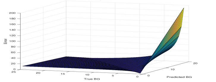
Fig 7: Target $err_{rLl}$ Loss Function. This function emphasizes loss when the model fails to predict hypoglycemic events. Here, “True BG” refers to BG_i+1 and “Predicted BG” refers to $\widehat{\hbox{{\sc BG}}_{i+1}}\ =\ M(\,x_{i},\,\Delta t_{i+1}\,)$. Note that the error is large when the true BG is very low, but the predicted $\widehat{\hbox{{\sc BG}}}$ is relatively high.

A.4 Experimental Results: Heat-Maps

This sub-appendix provides a set of heat-maps (Figs 8,  9,  10 and  11). The left half of each heat-map contains the datasets that adhere to our EP rules, while the right half contains those datasets that do not. Models (on the y axis) are sorted in terms of their average $err_{L1}$ error (over all 26 datasets), so that the model with the best average $err_{L1}$ error across all datasets appears at the top of these figures. Further, datasets $D_{e}$1 to $D_{e}$13 and $D_{a}$1 to $D_{a}$13 (in each half of these heat maps) are sorted horizontally, in increasing order of average $err_{L1}$ error across all models, with the left most dataset in each half having the smallest error. In Figure 8, the best model/dataset combination is found in the top left corner. More detailed results for these heat-maps are seen in Borle [25].

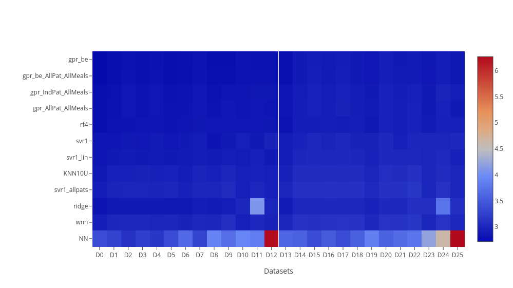
Fig 8: Average L1 Loss: Datasets vs. Models. Datasets using the EP criteria are on the left half of the bisecting white line. Each square represents the cross-validation L1 error, micro-averaged over patients.

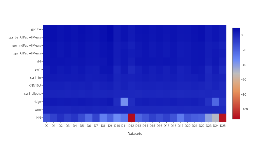
Fig 9: Percent Improvement in Average L1 Loss for Models vs. Baseline. Datasets using the EP criteria are on the left half of the bisecting white line. Each square corresponds with the percent change between the corresponding result in Figure 8 and the performance of $M_{ave}$.

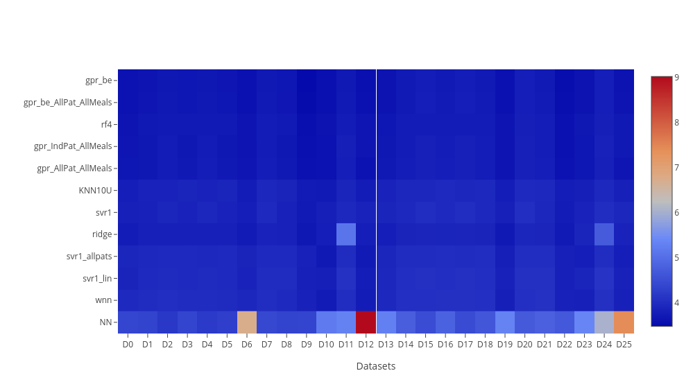
Fig 10: Average Relative L1 Loss: Datasets vs. Models. Datasets using the EP criteria are on the left half of the bisecting white line. Each square represents the cross-validation relative L1 error, micro-averaged over patients.

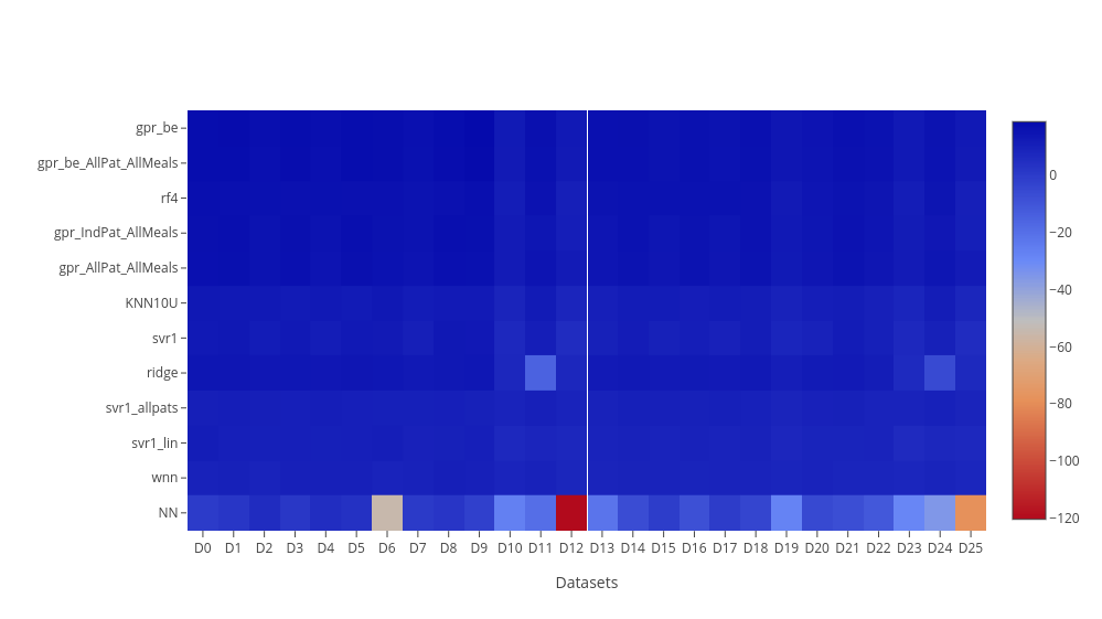
Fig 11: Percent Improvement in Average Relative L1 Loss for Models vs. Baseline. Datasets using the EP criteria are on the left half of the bisecting white line. Each square corresponds with the percent change between the corresponding result in Figure 10 and the performance of $M_{ave}$.

A.5 Experimental Results: Tables

Table 10: Losses Corresponding to Fig 8.

	$M^{w}_{gpr}$	$M^{ws}_{gpr}$	$M_{gpr}$	$M^{s}_{gpr}$	$M_{rf}$	$M_{svr}$	$M^{lin}_{svr}$	$M_{knn}$	$M^{s}_{svr}$	$M_{ridge}$	$M_{wnn}$	$M_{nn}$
$D_{e}$1	2.7	2.71	2.74	2.75	2.74	2.8	2.81	2.8	2.86	2.87	2.88	3.29
$D_{e}$2	2.79	2.79	2.82	2.83	2.83	2.88	2.9	2.88	2.91	2.93	2.95	3.8
$D_{e}$3	2.78	2.79	2.81	2.82	2.84	2.86	2.89	2.89	2.96	3.0	3.01	3.22
$D_{e}$4	2.79	2.79	2.82	2.82	2.84	2.86	2.9	2.89	2.97	3.0	3.01	3.37
$D_{e}$5	2.81	2.82	2.85	2.86	2.84	2.88	2.9	2.9	2.96	2.99	3.0	3.14
$D_{e}$6	2.78	2.78	2.81	2.81	2.83	2.84	2.89	2.88	2.96	2.98	3.01	3.2
$D_{e}$7	2.81	2.82	2.85	2.86	2.84	2.9	2.9	2.9	2.96	2.99	2.99	3.16
$D_{e}$8	2.79	2.79	2.82	2.82	2.84	2.84	2.9	2.9	2.97	3.0	3.0	3.44
$D_{e}$9	2.82	2.82	2.84	2.84	2.84	2.94	2.9	2.99	2.94	2.93	2.95	3.9
$D_{e}$10	2.82	2.83	2.86	2.86	2.87	2.91	2.92	2.92	2.98	3.0	3.02	3.31
$D_{e}$11	2.78	2.79	2.84	2.85	2.85	2.89	2.93	2.92	2.99	3.05	3.05	3.61
$D_{e}$12	2.84	2.84	2.87	2.88	2.88	2.87	2.93	2.93	2.99	3.03	3.0	3.64
$D_{e}$13	2.82	2.82	2.83	2.84	2.88	2.9	2.89	2.98	2.95	2.94	2.96	29.04
$D_{a}$1	2.78	2.78	2.83	2.83	2.82	2.9	2.9	2.89	2.94	2.97	2.99	3.58
$D_{a}$2	2.86	2.86	2.9	2.9	2.91	2.97	2.97	2.96	3.0	3.03	3.05	3.83
$D_{a}$3	2.89	2.9	2.92	2.93	2.94	2.97	3.0	3.01	3.07	3.12	3.12	3.47
$D_{a}$4	2.9	2.9	2.93	2.93	2.93	2.98	3.01	3.02	3.07	3.11	3.13	3.48
$D_{a}$5	2.92	2.93	2.96	2.97	2.93	3.01	3.03	3.02	3.07	3.1	3.12	3.35
$D_{a}$6	2.89	2.89	2.92	2.92	2.93	2.96	3.01	3.01	3.07	3.1	3.12	3.61
$D_{a}$7	2.92	2.93	2.96	2.97	2.93	3.02	3.03	3.02	3.07	3.1	3.11	3.38
$D_{a}$8	2.89	2.9	2.92	2.93	2.93	2.95	3.02	3.02	3.07	3.11	3.12	3.77
$D_{a}$9	2.87	2.87	2.89	2.89	2.91	3.0	2.97	3.09	3.0	3.0	3.0	4.14
$D_{a}$10	2.93	2.93	2.96	2.96	2.97	3.02	3.03	3.04	3.08	3.12	3.15	3.53
$D_{a}$11	2.9	2.9	2.95	2.96	2.96	3.0	3.02	3.1	3.12	3.16	3.17	4.22
$D_{a}$12	2.94	2.94	2.97	2.97	2.96	2.98	3.03	3.05	3.09	3.13	3.12	4.7
$D_{a}$13	2.87	2.87	2.89	2.89	2.94	2.96	2.95	3.06	3.01	3.0	3.01	6.1

See Table 8 for descriptions of the different datasets and Table 9 for descriptions of the models.

Table 11: Percentage Improvements Corresponding to Fig 9.

	$M^{w}_{gpr}$	$M^{ws}_{gpr}$	$M_{gpr}$	$M^{s}_{gpr}$	$M_{rf}$	$M_{svr}$	$M^{lin}_{svr}$	$M_{ridge}$	$M_{knn}$	$M^{s}_{svr}$	$M_{wnn}$	$M_{nn}$
$D_{e}$1	7.12	7.02	5.75	5.54	5.95	3.73	3.58	3.77	1.8	1.45	1.11	-13.15
$D_{e}$2	6.19	6.14	5.02	4.8	4.62	2.93	2.28	3.18	1.97	1.48	0.85	-27.86
$D_{e}$3	7.98	7.85	6.96	6.83	6.03	5.51	4.43	4.6	1.98	0.88	0.56	-6.35
$D_{e}$4	7.79	7.74	6.82	6.75	6.07	5.47	4.26	4.44	1.66	0.87	0.39	-11.52
$D_{e}$5	7.01	6.82	5.86	5.59	6.13	4.61	4.02	4.27	2.19	1.05	0.69	-3.69
$D_{e}$6	8.18	8.02	7.23	6.98	6.34	6.09	4.38	4.62	2.24	1.3	0.48	-5.91
$D_{e}$7	7.01	6.76	5.86	5.57	6.2	4.25	4.02	4.27	2.19	1.19	0.98	-4.47
$D_{e}$8	7.93	7.8	6.91	6.73	6.04	6.27	4.06	3.99	1.9	0.73	0.94	-13.7
$D_{e}$9	4.2	4.15	3.5	3.49	3.39	0.11	1.42	-1.55	0.01	0.16	-0.23	-32.75
$D_{e}$10	6.65	6.48	5.57	5.38	5.06	3.62	3.33	3.51	1.33	0.75	0.09	-9.39
$D_{e}$11	9.94	9.72	8.04	7.61	7.61	6.47	5.15	5.33	3.11	1.09	1.23	-16.83
$D_{e}$12	6.27	6.03	5.0	4.71	4.96	4.99	3.17	2.85	1.29	-0.13	0.72	-20.35
$D_{e}$13	4.1	3.99	3.7	3.53	2.15	1.19	1.8	-1.24	-0.4	-0.18	-0.75	-887.75
$D_{a}$1	6.14	6.08	4.63	4.49	4.79	2.14	2.13	2.37	0.9	-0.18	-0.73	-20.68
$D_{a}$2	4.97	4.9	3.69	3.53	3.31	1.27	1.31	1.59	0.5	-0.53	-1.49	-27.2
$D_{a}$3	7.02	6.97	6.1	6.0	5.62	4.57	3.54	3.27	1.42	-0.06	-0.26	-11.37
$D_{a}$4	6.9	6.86	5.91	5.83	5.78	4.42	3.34	2.97	1.35	-0.01	-0.52	-11.91
$D_{a}$5	6.07	5.93	4.84	4.61	6.04	3.33	2.83	2.84	1.49	0.28	-0.28	-7.63
$D_{a}$6	7.23	7.07	6.34	6.1	5.96	4.96	3.43	3.27	1.51	0.38	-0.12	-15.97
$D_{a}$7	6.07	5.9	4.84	4.59	6.05	2.89	2.83	2.84	1.49	0.35	0.06	-8.41
$D_{a}$8	7.13	6.93	6.22	5.97	5.84	5.4	3.13	2.99	1.33	-0.01	-0.03	-20.94
$D_{a}$9	4.21	4.2	3.29	3.25	2.8	-0.19	0.56	-3.19	-0.22	-0.15	-0.16	-38.48
$D_{a}$10	5.95	5.85	4.92	4.79	4.73	3.05	2.72	2.46	0.93	-0.17	-1.19	-13.24
$D_{a}$11	7.91	7.81	6.26	5.99	6.17	4.73	4.22	1.68	1.1	-0.39	-0.74	-34.05
$D_{a}$12	5.64	5.53	4.66	4.49	4.8	4.47	2.55	2.15	0.75	-0.59	-0.27	-51.06
$D_{a}$13	4.11	4.0	3.51	3.36	1.62	1.1	1.47	-2.33	-0.69	-0.46	-0.61	-103.85

See Table 8 for descriptions of the different datasets and Table 9 for descriptions of the models.

Table 12: Losses Corresponding to Fig 10.

	$M^{w}_{gpr}$	$M^{ws}_{gpr}$	$M_{gpr}$	$M_{rf}$	$M^{s}_{gpr}$	$M_{ridge}$	$M_{knn}$	$M_{svr}$	$M^{s}_{svr}$	$M_{wnn}$	$M^{lin}_{svr}$	$M_{nn}$
$D_{e}$1	3.61	3.61	3.65	3.64	3.66	3.76	3.81	3.81	3.9	3.95	3.88	4.62
$D_{e}$2	3.62	3.62	3.68	3.65	3.69	3.77	3.78	3.82	3.89	3.97	3.9	4.6
$D_{e}$3	3.67	3.67	3.71	3.75	3.72	3.83	3.91	3.88	3.99	4.0	3.99	4.28
$D_{e}$4	3.67	3.68	3.72	3.75	3.72	3.84	3.92	3.88	3.99	4.02	3.99	4.3
$D_{e}$5	3.71	3.72	3.77	3.74	3.78	3.85	3.89	3.93	3.98	4.01	4.0	4.24
$D_{e}$6	3.66	3.67	3.7	3.74	3.72	3.83	3.89	3.85	3.96	4.03	3.99	4.27
$D_{e}$7	3.71	3.73	3.77	3.73	3.78	3.85	3.89	3.93	3.97	4.0	4.0	4.26
$D_{e}$8	3.67	3.68	3.71	3.75	3.72	3.86	3.91	3.85	3.99	4.02	4.02	4.37
$D_{e}$9	3.58	3.58	3.6	3.6	3.6	3.77	3.74	3.81	3.71	3.74	3.79	4.79
$D_{e}$10	3.73	3.74	3.78	3.8	3.79	3.87	3.94	3.98	3.99	4.03	4.02	4.41
$D_{e}$11	3.48	3.5	3.57	3.57	3.59	3.69	3.74	3.72	3.86	3.85	3.84	4.68
$D_{e}$12	3.75	3.76	3.8	3.8	3.81	3.89	3.95	3.93	4.03	4.0	4.05	4.73
$D_{e}$13	3.58	3.58	3.59	3.64	3.6	3.77	3.77	3.77	3.73	3.76	3.77	6.02
$D_{a}$1	3.64	3.64	3.71	3.68	3.72	3.81	3.89	3.9	3.91	3.93	3.95	4.73
$D_{a}$2	3.62	3.62	3.67	3.66	3.67	3.75	3.8	3.86	3.81	3.85	3.88	4.73
$D_{a}$3	3.75	3.75	3.78	3.79	3.79	3.9	3.98	3.97	4.03	4.06	4.05	4.66
$D_{a}$4	3.75	3.75	3.79	3.79	3.79	3.91	3.98	3.98	4.03	4.08	4.06	4.82
$D_{a}$5	3.79	3.79	3.84	3.79	3.85	3.92	3.96	4.02	4.02	4.07	4.08	4.45
$D_{a}$6	3.74	3.74	3.77	3.78	3.78	3.9	3.96	3.95	4.01	4.06	4.05	4.63
$D_{a}$7	3.79	3.8	3.84	3.78	3.85	3.92	3.96	4.03	4.02	4.04	4.08	4.48
$D_{a}$8	3.75	3.75	3.78	3.8	3.79	3.93	3.98	3.94	4.03	4.09	4.09	4.78
$D_{a}$9	3.63	3.63	3.66	3.69	3.66	3.88	3.81	3.87	3.78	3.84	3.88	5.35
$D_{a}$10	3.8	3.8	3.84	3.82	3.85	3.93	4.0	4.05	4.04	4.05	4.09	4.68
$D_{a}$11	3.55	3.56	3.61	3.6	3.62	3.73	3.78	3.78	3.83	3.88	3.84	4.73
$D_{a}$12	3.82	3.82	3.86	3.85	3.87	3.97	4.02	4.01	4.06	4.07	4.13	11.06
$D_{a}$13	3.63	3.64	3.65	3.72	3.66	3.86	3.84	3.82	3.8	3.85	3.85	7.52

See Table 8 for descriptions of the different datasets and Table 9 for descriptions of the models. Here all values are multiplied by 10 so that they are the same order of magnitude as in Table 20.

Table 13: Percentage Improvements Corresponding to Fig 11.

	$M^{w}_{gpr}$	$M^{ws}_{gpr}$	$M_{gpr}$	$M_{rf}$	$M^{s}_{gpr}$	$M_{ridge}$	$M_{knn}$	$M_{svr}$	$M^{s}_{svr}$	$M^{lin}_{svr}$	$M_{wnn}$	$M_{nn}$
$D_{e}$1	17.53	17.45	16.52	16.76	16.33	14.19	12.9	12.99	10.96	11.37	9.68	-5.64
$D_{e}$2	16.69	16.63	15.34	16.03	15.13	13.16	12.99	12.06	10.56	10.16	8.59	-5.95
$D_{e}$3	17.97	17.79	16.9	16.16	16.71	14.2	12.47	13.16	10.83	10.76	10.4	4.17
$D_{e}$4	17.81	17.73	16.79	16.15	16.72	14.04	12.3	13.13	10.73	10.78	10.07	3.82
$D_{e}$5	16.91	16.73	15.64	16.42	15.39	13.89	13.0	12.14	10.87	10.58	10.32	5.19
$D_{e}$6	18.16	17.95	17.16	16.34	16.86	14.21	13.01	13.76	11.31	10.79	9.93	4.5
$D_{e}$7	16.91	16.64	15.64	16.43	15.32	13.89	13.0	11.96	11.1	10.58	10.39	4.67
$D_{e}$8	17.85	17.7	16.92	16.07	16.73	13.59	12.45	13.77	10.69	10.16	10.12	2.34
$D_{e}$9	12.68	12.61	12.07	12.09	12.06	7.84	8.65	7.01	9.38	7.43	8.72	-16.97
$D_{e}$10	16.57	16.38	15.46	14.89	15.26	13.36	11.91	11.01	10.62	10.03	9.82	1.38
$D_{e}$11	18.97	18.7	16.87	16.89	16.42	14.1	12.95	13.47	10.26	10.72	10.5	-8.95
$D_{e}$12	16.13	15.86	15.06	14.9	14.73	12.82	11.7	12.11	9.8	9.42	10.51	-5.72
$D_{e}$13	12.65	12.49	12.27	11.01	12.06	7.96	7.93	7.99	9.01	7.83	8.31	-46.92
$D_{a}$1	15.85	15.83	14.3	14.9	14.17	12.11	10.15	9.93	9.79	8.86	9.22	-9.33
$D_{a}$2	13.7	13.63	12.54	12.67	12.41	10.56	9.29	7.96	9.05	7.39	8.14	-12.83
$D_{a}$3	16.61	16.54	15.77	15.59	15.66	13.19	11.36	11.66	10.18	9.73	9.56	-3.7
$D_{a}$4	16.55	16.5	15.63	15.71	15.56	13.02	11.39	11.41	10.22	9.71	9.15	-7.34
$D_{a}$5	15.68	15.54	14.52	15.67	14.31	12.76	11.85	10.45	10.48	9.26	9.36	0.96
$D_{a}$6	16.84	16.65	16.03	15.85	15.76	13.17	11.84	12.02	10.71	9.75	9.58	-3.01
$D_{a}$7	15.68	15.51	14.52	15.91	14.28	12.76	11.85	10.18	10.62	9.26	10.0	0.23
$D_{a}$8	16.64	16.43	15.83	15.36	15.59	12.6	11.44	12.2	10.29	9.07	9.0	-6.37
$D_{a}$9	12.88	12.89	12.11	11.57	12.1	6.83	8.53	7.19	9.21	6.86	7.8	-28.32
$D_{a}$10	15.47	15.35	14.51	14.86	14.38	12.45	11.04	9.85	10.0	9.02	9.74	-4.16
$D_{a}$11	15.88	15.74	14.61	14.71	14.33	11.55	10.49	10.47	9.25	9.15	8.15	-11.98
$D_{a}$12	15.02	14.9	14.15	14.34	13.95	11.59	10.63	10.81	9.73	7.97	9.49	-146.23
$D_{a}$13	12.89	12.76	12.47	10.71	12.29	7.49	7.98	8.28	8.85	7.64	7.68	-80.39

See Table 8 for descriptions of the different datasets and Table 9 for descriptions of the models.

Table 14: Losses Using gMAD.

	$M_{svr}$	$M^{w}_{gpr}$	$M^{ws}_{gpr}$	$M_{rf}$	$M_{gpr}$	$M^{s}_{gpr}$	$M^{lin}_{svr}$	$M_{ridge}$	$M_{knn}$	$M^{s}_{svr}$	$M_{wnn}$	$M_{nn}$
$D_{e}$1	5.03	4.98	4.99	5.05	5.08	5.09	5.12	5.19	5.24	5.37	5.38	5.75
$D_{e}$2	5.13	5.09	5.09	5.18	5.17	5.17	5.21	5.26	5.28	5.4	5.42	6.43
$D_{e}$3	5.16	5.19	5.2	5.31	5.25	5.26	5.32	5.41	5.48	5.69	5.68	5.68
$D_{e}$4	5.16	5.2	5.21	5.31	5.26	5.26	5.33	5.42	5.49	5.7	5.7	6.1
$D_{e}$5	5.21	5.25	5.26	5.3	5.32	5.33	5.33	5.41	5.47	5.6	5.7	5.58
$D_{e}$6	5.13	5.17	5.18	5.29	5.23	5.25	5.32	5.41	5.47	5.65	5.68	5.67
$D_{e}$7	5.22	5.25	5.27	5.3	5.32	5.33	5.33	5.41	5.47	5.62	5.66	5.63
$D_{e}$8	5.14	5.2	5.21	5.31	5.27	5.28	5.36	5.47	5.5	5.67	5.66	5.97
$D_{e}$9	5.2	5.18	5.18	5.17	5.22	5.22	5.15	5.32	5.34	5.49	5.46	6.4
$D_{e}$10	5.27	5.27	5.28	5.37	5.34	5.35	5.4	5.48	5.51	5.7	5.71	5.82
$D_{e}$11	5.1	5.08	5.09	5.2	5.18	5.2	5.23	5.33	5.41	5.63	5.59	6.04
$D_{e}$12	5.25	5.33	5.34	5.39	5.42	5.43	5.46	5.56	5.54	5.69	5.68	6.37
$D_{e}$13	5.15	5.18	5.18	5.23	5.21	5.22	5.23	5.4	5.35	5.49	5.49	31.86
$D_{a}$1	5.2	5.14	5.14	5.19	5.25	5.25	5.29	5.36	5.4	5.6	5.61	6.17
$D_{a}$2	5.28	5.23	5.23	5.3	5.32	5.33	5.33	5.42	5.44	5.63	5.65	6.44
$D_{a}$3	5.36	5.4	5.41	5.48	5.47	5.47	5.52	5.64	5.7	5.94	5.94	6.09
$D_{a}$4	5.37	5.41	5.41	5.47	5.48	5.49	5.53	5.65	5.69	5.95	5.92	6.11
$D_{a}$5	5.43	5.46	5.47	5.46	5.55	5.57	5.55	5.65	5.69	5.86	5.93	5.91
$D_{a}$6	5.34	5.38	5.4	5.46	5.45	5.47	5.52	5.64	5.69	5.91	5.89	6.2
$D_{a}$7	5.45	5.46	5.48	5.45	5.55	5.57	5.55	5.65	5.69	5.88	5.91	5.93
$D_{a}$8	5.33	5.4	5.41	5.47	5.47	5.48	5.57	5.68	5.7	5.92	5.92	6.42
$D_{a}$9	5.33	5.28	5.28	5.33	5.34	5.34	5.29	5.49	5.47	5.62	5.57	6.81
$D_{a}$10	5.46	5.47	5.48	5.53	5.55	5.56	5.58	5.69	5.72	5.95	5.99	6.18
$D_{a}$11	5.3	5.29	5.3	5.38	5.41	5.42	5.38	5.59	5.67	5.88	5.84	6.79
$D_{a}$12	5.42	5.52	5.53	5.55	5.6	5.61	5.64	5.76	5.74	5.93	5.93	7.73
$D_{a}$13	5.26	5.28	5.28	5.37	5.32	5.33	5.35	5.55	5.49	5.61	5.58	9.04

See Table 8 for descriptions of the different datasets and Table 9 for descriptions of the models.

Table 15: Percentage Improvements for gMAD.

	$M_{svr}$	$M^{w}_{gpr}$	$M^{ws}_{gpr}$	$M_{rf}$	$M_{gpr}$	$M^{s}_{gpr}$	$M^{lin}_{svr}$	$M_{ridge}$	$M_{knn}$	$M^{s}_{svr}$	$M_{wnn}$	$M_{nn}$
$D_{e}$1	5.41	6.28	6.19	5.07	4.43	4.23	3.73	2.35	1.39	-1.0	-1.15	-8.12
$D_{e}$2	3.29	4.02	4.01	2.45	2.62	2.46	1.8	0.91	0.57	-1.73	-2.17	-21.15
$D_{e}$3	7.47	6.9	6.69	4.73	5.81	5.67	4.52	2.93	1.7	-2.08	-1.95	-1.99
$D_{e}$4	7.38	6.68	6.57	4.77	5.61	5.56	4.36	2.81	1.46	-2.23	-2.35	-9.52
$D_{e}$5	6.58	5.81	5.56	4.97	4.6	4.28	4.44	2.85	1.8	-0.43	-2.27	-0.07
$D_{e}$6	8.03	7.2	6.97	5.07	6.17	5.89	4.6	3.02	1.83	-1.37	-2.0	-1.82
$D_{e}$7	6.41	5.81	5.5	4.94	4.6	4.29	4.44	2.85	1.8	-0.76	-1.49	-1.1
$D_{e}$8	7.78	6.72	6.59	4.72	5.5	5.35	3.79	1.92	1.37	-1.62	-1.41	-7.01
$D_{e}$9	1.36	1.79	1.72	1.85	1.0	0.98	2.23	-0.93	-1.26	-4.19	-3.6	-21.35
$D_{e}$10	5.43	5.4	5.19	3.63	4.19	3.97	3.16	1.7	1.06	-2.32	-2.54	-4.43
$D_{e}$11	6.54	6.94	6.73	4.74	5.03	4.65	4.09	2.35	0.87	-3.16	-2.35	-10.64
$D_{e}$12	5.9	4.49	4.31	3.27	2.85	2.61	2.07	0.07	0.59	-2.08	-1.9	-14.29
$D_{e}$13	2.37	1.79	1.68	0.82	1.28	1.07	0.85	-2.49	-1.47	-4.03	-4.12	-504.3
$D_{a}$1	4.59	5.7	5.67	4.83	3.76	3.63	2.95	1.58	0.85	-2.83	-2.89	-13.21
$D_{a}$2	2.45	3.29	3.27	1.98	1.65	1.52	1.47	-0.14	-0.62	-4.07	-4.34	-19.05
$D_{a}$3	6.94	6.24	6.14	4.87	5.08	4.98	4.09	2.07	1.11	-3.21	-3.06	-5.73
$D_{a}$4	6.72	6.07	6.0	5.07	4.83	4.76	3.92	1.89	1.25	-3.23	-2.81	-6.07
$D_{a}$5	5.64	5.15	4.96	5.24	3.63	3.35	3.71	1.89	1.24	-1.71	-3.0	-2.58
$D_{a}$6	7.35	6.51	6.29	5.18	5.41	5.11	4.08	2.12	1.24	-2.56	-2.34	-7.68
$D_{a}$7	5.37	5.15	4.9	5.31	3.63	3.32	3.71	1.89	1.24	-2.0	-2.67	-2.94
$D_{a}$8	7.5	6.22	6.05	5.11	5.07	4.84	3.38	1.36	0.99	-2.66	-2.81	-11.38
$D_{a}$9	1.14	2.03	2.02	1.13	0.88	0.85	1.73	-1.85	-1.55	-4.29	-3.46	-26.43
$D_{a}$10	5.21	5.02	4.88	3.9	3.69	3.53	3.09	1.23	0.75	-3.36	-4.06	-7.38
$D_{a}$11	5.62	5.66	5.6	4.15	3.63	3.38	4.11	0.35	-1.02	-4.77	-4.08	-21.08
$D_{a}$12	5.98	4.13	4.07	3.76	2.86	2.7	2.16	-0.08	0.3	-2.92	-2.91	-34.21
$D_{a}$13	2.3	2.05	1.96	0.35	1.25	1.06	0.72	-3.01	-1.83	-4.22	-3.55	-67.75

See Table 8 for descriptions of the different datasets and Table 9 for descriptions of the models.

Table 16: Losses Using gMARD

	$M^{w}_{gpr}$	$M^{ws}_{gpr}$	$M_{rf}$	$M_{gpr}$	$M^{s}_{gpr}$	$M_{svr}$	$M_{ridge}$	$M_{knn}$	$M^{lin}_{svr}$	$M^{s}_{svr}$	$M_{wnn}$	$M_{nn}$
$D_{e}$1	6.88	6.89	6.95	7.01	7.02	7.1	7.22	7.23	7.38	7.58	7.68	8.63
$D_{e}$2	6.74	6.74	6.78	6.88	6.89	6.97	7.06	6.96	7.21	7.33	7.44	7.99
$D_{e}$3	7.1	7.12	7.29	7.21	7.23	7.32	7.49	7.51	7.7	7.88	7.9	7.94
$D_{e}$4	7.12	7.13	7.27	7.22	7.23	7.33	7.5	7.52	7.7	7.9	7.92	7.92
$D_{e}$5	7.2	7.23	7.25	7.33	7.35	7.41	7.5	7.47	7.69	7.75	7.94	7.89
$D_{e}$6	7.08	7.1	7.28	7.18	7.21	7.27	7.49	7.47	7.69	7.81	7.94	7.89
$D_{e}$7	7.2	7.23	7.25	7.33	7.36	7.41	7.5	7.47	7.69	7.76	7.91	7.94
$D_{e}$8	7.13	7.14	7.3	7.23	7.24	7.3	7.58	7.54	7.79	7.84	7.93	8.11
$D_{e}$9	6.65	6.66	6.64	6.71	6.71	6.85	6.83	6.9	6.87	7.04	7.04	8.11
$D_{e}$10	7.24	7.26	7.4	7.35	7.37	7.53	7.57	7.55	7.78	7.91	7.96	8.22
$D_{e}$11	6.48	6.5	6.63	6.64	6.67	6.74	6.87	6.86	7.05	7.22	7.19	7.91
$D_{e}$12	7.33	7.34	7.42	7.45	7.48	7.5	7.69	7.62	7.92	7.88	7.91	8.64
$D_{e}$13	6.65	6.66	6.71	6.68	6.7	6.77	6.94	6.94	6.95	7.03	7.04	9.39
$D_{a}$1	6.97	6.97	7.01	7.15	7.16	7.28	7.33	7.44	7.51	7.67	7.68	8.48
$D_{a}$2	6.75	6.75	6.8	6.87	6.88	7.03	7.01	7.06	7.16	7.24	7.28	8.2
$D_{a}$3	7.26	7.27	7.34	7.35	7.37	7.48	7.61	7.69	7.82	8.01	8.05	8.53
$D_{a}$4	7.26	7.27	7.33	7.37	7.38	7.51	7.62	7.66	7.82	8.02	8.07	8.63
$D_{a}$5	7.35	7.37	7.34	7.48	7.51	7.6	7.63	7.63	7.84	7.88	8.08	8.23
$D_{a}$6	7.23	7.25	7.32	7.32	7.35	7.45	7.61	7.63	7.81	7.95	8.04	8.44
$D_{a}$7	7.35	7.37	7.32	7.48	7.51	7.6	7.63	7.63	7.84	7.9	8.0	8.3
$D_{a}$8	7.27	7.29	7.36	7.36	7.39	7.46	7.7	7.68	7.91	7.96	8.08	8.65
$D_{a}$9	6.81	6.81	6.85	6.89	6.88	7.02	7.06	7.1	7.08	7.23	7.28	9.06
$D_{a}$10	7.37	7.38	7.41	7.48	7.5	7.66	7.68	7.69	7.89	8.03	8.03	8.57
$D_{a}$11	6.6	6.61	6.67	6.72	6.73	6.84	6.9	6.98	7.02	7.22	7.26	8.05
$D_{a}$12	7.46	7.47	7.47	7.57	7.59	7.63	7.83	7.76	8.06	7.98	8.03	15.13
$D_{a}$13	6.8	6.81	6.91	6.84	6.86	6.94	7.14	7.13	7.14	7.24	7.27	11.0

See Table 8 for descriptions of the different datasets and Table 9 for descriptions of the models. Here all values are multiplied by 10 so that they are the same order of magnitude as in Table 20.

Table 17: Percentage Improvements Corresponding to gMARD.

	$M^{w}_{gpr}$	$M^{ws}_{gpr}$	$M_{rf}$	$M_{gpr}$	$M^{s}_{gpr}$	$M_{svr}$	$M_{ridge}$	$M_{knn}$	$M^{lin}_{svr}$	$M^{s}_{svr}$	$M_{wnn}$	$M_{nn}$
$D_{e}$1	18.38	18.28	17.53	16.81	16.63	15.73	14.29	14.18	12.44	10.05	8.87	-2.41
$D_{e}$2	16.37	16.35	15.83	14.59	14.45	13.49	12.39	13.57	10.54	9.04	7.65	0.76
$D_{e}$3	18.29	18.02	16.06	17.05	16.85	15.71	13.76	13.52	11.37	9.33	9.13	8.61
$D_{e}$4	18.08	17.93	16.27	16.88	16.81	15.58	13.64	13.5	11.41	9.05	8.86	8.86
$D_{e}$5	17.09	16.84	16.54	15.64	15.36	14.67	13.67	14.06	11.49	10.84	8.65	9.22
$D_{e}$6	18.56	18.27	16.22	17.41	17.04	16.32	13.84	14.03	11.52	10.12	8.66	9.18
$D_{e}$7	17.09	16.76	16.52	15.64	15.29	14.69	13.67	14.06	11.49	10.64	9.0	8.61
$D_{e}$8	18.03	17.84	16.03	16.84	16.66	15.98	12.77	13.29	10.41	9.84	8.82	6.75
$D_{e}$9	11.56	11.47	11.72	10.82	10.81	8.9	9.18	8.32	8.65	6.42	6.37	-7.75
$D_{e}$10	16.68	16.43	14.87	15.38	15.14	13.35	12.84	13.07	10.46	8.98	8.36	5.35
$D_{e}$11	17.28	17.02	15.34	15.17	14.77	13.99	12.29	12.4	10.01	7.78	8.15	-1.04
$D_{e}$12	15.72	15.51	14.61	14.26	13.98	13.72	11.35	12.34	8.88	9.35	9.02	0.62
$D_{e}$13	11.65	11.47	10.81	11.15	10.89	10.0	7.79	7.81	7.65	6.49	6.36	-24.83
$D_{a}$1	16.96	16.95	16.46	14.85	14.73	13.24	12.71	11.35	10.48	8.62	8.47	-1.04
$D_{a}$2	13.43	13.42	12.78	11.9	11.81	9.83	10.13	9.48	8.2	7.1	6.7	-5.09
$D_{a}$3	17.1	16.98	16.09	15.98	15.85	14.53	13.05	12.19	10.66	8.47	8.07	2.52
$D_{a}$4	17.01	16.91	16.24	15.78	15.7	14.16	12.98	12.52	10.69	8.41	7.86	1.39
$D_{a}$5	16.03	15.84	16.12	14.5	14.25	13.2	12.82	12.88	10.45	9.93	7.74	5.95
$D_{a}$6	17.39	17.13	16.38	16.33	15.98	14.92	13.08	12.85	10.77	9.23	8.2	3.61
$D_{a}$7	16.03	15.8	16.41	14.5	14.21	13.12	12.82	12.88	10.46	9.72	8.63	5.17
$D_{a}$8	16.99	16.8	15.89	15.89	15.65	14.8	12.08	12.32	9.68	9.12	7.73	1.19
$D_{a}$9	11.96	11.98	11.45	10.97	10.98	9.21	8.7	8.14	8.49	6.45	5.81	-17.13
$D_{a}$10	15.81	15.63	15.32	14.5	14.34	12.46	12.3	12.11	9.85	8.22	8.2	2.13
$D_{a}$11	14.5	14.4	13.59	13.04	12.79	11.45	10.59	9.64	9.07	6.54	6.03	-4.28
$D_{a}$12	14.74	14.69	14.68	13.53	13.36	12.81	10.49	11.35	7.94	8.88	8.34	-72.84
$D_{a}$13	12.11	11.99	10.67	11.53	11.32	10.31	7.69	7.8	7.65	6.43	6.01	-42.24

See Table 8 for descriptions of the different datasets and Table 9 for descriptions of the models.

Table 18: Losses Using RMSE.

	$M^{w}_{gpr}$	$M^{ws}_{gpr}$	$M_{gpr}$	$M^{s}_{gpr}$	$M_{rf}$	$M_{svr}$	$M^{lin}_{svr}$	$M_{knn}$	$M_{wnn}$	$M^{s}_{svr}$	$M_{ridge}$	$M_{nn}$
$D_{e}$1	3.47	3.47	3.52	3.53	3.52	3.59	3.57	3.66	3.64	3.64	3.58	4.37
$D_{e}$2	3.57	3.57	3.6	3.61	3.63	3.69	3.75	3.73	3.72	3.7	3.65	6.71
$D_{e}$3	3.59	3.6	3.62	3.63	3.66	3.66	3.67	3.81	3.83	3.84	3.69	4.24
$D_{e}$4	3.6	3.6	3.63	3.63	3.66	3.67	3.68	3.83	3.85	3.84	3.7	6.02
$D_{e}$5	3.63	3.63	3.66	3.67	3.66	3.69	3.69	3.81	3.83	3.85	3.71	4.17
$D_{e}$6	3.59	3.59	3.61	3.62	3.65	3.65	3.68	3.81	3.84	3.83	3.7	4.35
$D_{e}$7	3.63	3.63	3.66	3.67	3.66	3.71	3.69	3.81	3.81	3.84	3.71	4.24
$D_{e}$8	3.6	3.6	3.63	3.63	3.66	3.65	3.69	3.82	3.83	3.86	3.72	5.76
$D_{e}$9	3.64	3.64	3.66	3.66	3.66	3.76	3.74	3.78	3.78	3.77	4.73	5.94
$D_{e}$10	3.64	3.64	3.67	3.68	3.69	3.73	3.71	3.84	3.86	3.84	3.73	4.6
$D_{e}$11	3.58	3.58	3.63	3.65	3.66	3.68	3.7	3.82	3.85	3.88	3.72	6.61
$D_{e}$12	3.65	3.65	3.69	3.7	3.7	3.68	3.72	3.84	3.84	3.88	3.75	6.07
$D_{e}$13	3.64	3.64	3.65	3.65	3.71	3.71	3.69	3.78	3.8	3.78	4.52	254.95
$D_{a}$1	3.58	3.58	3.63	3.63	3.63	3.71	3.71	3.76	3.81	3.78	3.71	5.56
$D_{a}$2	3.66	3.66	3.7	3.71	3.72	3.78	3.82	3.83	3.87	3.85	3.78	6.48
$D_{a}$3	3.72	3.73	3.75	3.76	3.78	3.8	3.82	3.94	3.99	3.99	3.95	5.01
$D_{a}$4	3.73	3.73	3.76	3.77	3.78	3.81	3.83	3.94	3.99	3.98	4.11	5.17
$D_{a}$5	3.76	3.76	3.8	3.81	3.77	3.85	3.86	3.94	3.98	3.99	3.96	5.04
$D_{a}$6	3.72	3.72	3.75	3.76	3.77	3.79	3.83	3.94	3.98	3.98	3.94	6.64
$D_{a}$7	3.76	3.77	3.8	3.81	3.77	3.87	3.86	3.94	3.97	3.98	3.96	5.02
$D_{a}$8	3.72	3.73	3.75	3.76	3.78	3.78	3.84	3.95	3.98	3.99	3.88	9.06
$D_{a}$9	3.7	3.7	3.73	3.73	3.74	3.84	3.84	3.86	3.85	3.84	5.16	7.55
$D_{a}$10	3.76	3.77	3.8	3.8	3.81	3.86	3.85	3.96	4.02	3.98	4.07	5.7
$D_{a}$11	3.71	3.71	3.77	3.78	3.78	3.82	3.83	3.98	4.01	4.02	5.81	13.15
$D_{a}$12	3.77	3.78	3.81	3.81	3.82	3.8	3.86	3.97	3.99	4.01	3.9	20.01
$D_{a}$13	3.7	3.7	3.72	3.72	3.79	3.79	3.76	3.86	3.86	3.86	4.86	41.78

See Table 8 for descriptions of the different datasets and Table 9 for descriptions of the models.

Table 19: Percentage Improvements for RMSE.

	$M^{w}_{gpr}$	$M^{ws}_{gpr}$	$M_{gpr}$	$M^{s}_{gpr}$	$M_{rf}$	$M_{svr}$	$M^{lin}_{svr}$	$M_{knn}$	$M^{s}_{svr}$	$M_{wnn}$	$M_{ridge}$	$M_{nn}$
$D_{e}$1	2.98	2.93	1.65	1.5	1.6	-0.3	0.38	-2.38	-1.62	-1.75	0.05	-22.06
$D_{e}$2	2.06	2.18	1.22	1.2	0.61	-1.05	-2.65	-2.15	-1.39	-1.95	-0.14	-83.81
$D_{e}$3	4.29	4.15	3.53	3.36	2.55	2.47	2.24	-1.51	-2.31	-2.16	1.59	-12.86
$D_{e}$4	4.05	3.97	3.3	3.2	2.46	2.2	2.0	-1.97	-2.21	-2.52	1.41	-60.39
$D_{e}$5	3.39	3.26	2.53	2.33	2.54	1.56	1.62	-1.45	-2.51	-2.18	1.16	-11.05
$D_{e}$6	4.45	4.24	3.75	3.48	2.74	2.77	2.02	-1.43	-2.04	-2.3	1.46	-15.86
$D_{e}$7	3.39	3.15	2.53	2.27	2.57	1.04	1.62	-1.45	-2.36	-1.6	1.16	-13.0
$D_{e}$8	4.14	4.02	3.3	3.18	2.44	2.88	1.76	-1.73	-2.71	-1.95	0.88	-53.49
$D_{e}$9	0.93	0.89	0.35	0.31	0.24	-2.47	-2.02	-2.95	-2.77	-3.0	-28.94	-61.96
$D_{e}$10	3.11	2.94	2.19	1.99	1.63	0.64	1.23	-2.24	-2.32	-2.89	0.61	-22.57
$D_{e}$11	6.25	6.05	4.81	4.39	4.17	3.43	2.88	-0.26	-1.63	-1.07	2.54	-73.25
$D_{e}$12	2.84	2.67	1.7	1.47	1.39	1.96	1.01	-2.26	-3.31	-2.24	-0.1	-61.66
$D_{e}$13	0.8	0.71	0.61	0.48	-0.98	-1.2	-0.6	-3.09	-3.03	-3.54	-23.2	-6846.22
$D_{a}$1	2.49	2.49	1.11	1.03	1.18	-1.01	-0.99	-2.54	-3.04	-3.73	-1.1	-51.5
$D_{a}$2	1.8	1.85	0.64	0.62	0.2	-1.51	-2.44	-2.71	-3.17	-3.79	-1.28	-73.68
$D_{a}$3	3.67	3.61	2.87	2.75	2.29	1.69	1.1	-1.93	-3.12	-3.26	-2.26	-29.54
$D_{a}$4	3.49	3.43	2.64	2.53	2.3	1.45	0.82	-2.07	-3.0	-3.12	-6.4	-33.72
$D_{a}$5	2.72	2.6	1.63	1.46	2.52	0.47	0.13	-1.99	-3.18	-2.93	-2.55	-30.45
$D_{a}$6	3.83	3.62	3.06	2.78	2.43	1.92	0.88	-1.99	-2.87	-2.94	-1.85	-71.78
$D_{a}$7	2.72	2.53	1.63	1.39	2.51	-0.07	0.13	-1.99	-3.07	-2.69	-2.55	-29.79
$D_{a}$8	3.68	3.53	2.87	2.67	2.32	2.28	0.66	-2.11	-3.32	-2.91	-0.26	-134.27
$D_{a}$9	1.04	1.03	0.17	0.13	-0.27	-2.68	-2.7	-3.23	-2.92	-3.11	-38.13	-102.02
$D_{a}$10	2.69	2.58	1.77	1.6	1.34	0.25	0.44	-2.44	-3.1	-4.01	-5.4	-47.41
$D_{a}$11	5.02	4.94	3.51	3.28	3.3	2.1	1.91	-1.91	-2.9	-2.74	-48.79	-236.69
$D_{a}$12	2.41	2.34	1.52	1.36	1.29	1.61	0.03	-2.6	-3.74	-3.17	-0.91	-417.57
$D_{a}$13	1.01	0.93	0.51	0.38	-1.48	-1.46	-0.76	-3.39	-3.28	-3.48	-30.03	-1018.57

See Table 8 for descriptions of the different datasets and Table 9 for descriptions of the models.

Table 20: Losses Using gRMSE.

	$M^{w}_{gpr}$	$M^{ws}_{gpr}$	$M_{svr}$	$M_{gpr}$	$M^{s}_{gpr}$	$M_{rf}$	$M^{lin}_{svr}$	$M_{knn}$	$M_{wnn}$	$M^{s}_{svr}$	$M_{ridge}$	$M_{nn}$
$D_{e}$1	4.86	4.87	4.96	4.94	4.95	4.93	4.97	5.12	5.14	5.13	5.02	5.88
$D_{e}$2	5.0	4.99	5.09	5.05	5.04	5.07	5.15	5.18	5.22	5.2	5.1	8.62
$D_{e}$3	5.06	5.07	5.07	5.1	5.11	5.16	5.14	5.35	5.44	5.45	5.21	5.72
$D_{e}$4	5.07	5.08	5.09	5.11	5.12	5.16	5.15	5.37	5.46	5.45	5.22	8.68
$D_{e}$5	5.11	5.12	5.12	5.16	5.17	5.15	5.16	5.34	5.45	5.43	5.23	5.62
$D_{e}$6	5.05	5.06	5.06	5.09	5.1	5.15	5.15	5.34	5.44	5.43	5.22	5.92
$D_{e}$7	5.11	5.12	5.14	5.16	5.17	5.16	5.16	5.34	5.41	5.43	5.23	5.78
$D_{e}$8	5.07	5.08	5.07	5.12	5.13	5.16	5.18	5.36	5.42	5.46	5.26	7.28
$D_{e}$9	5.1	5.1	5.17	5.13	5.13	5.11	5.14	5.27	5.33	5.34	6.12	7.35
$D_{e}$10	5.13	5.13	5.17	5.18	5.19	5.21	5.2	5.38	5.47	5.45	5.27	6.1
$D_{e}$11	4.99	5.0	5.05	5.07	5.09	5.09	5.11	5.31	5.38	5.43	5.18	8.06
$D_{e}$12	5.15	5.16	5.13	5.22	5.23	5.23	5.24	5.4	5.45	5.48	5.32	7.63
$D_{e}$13	5.1	5.11	5.11	5.12	5.12	5.17	5.14	5.27	5.36	5.34	5.97	256.36
$D_{a}$1	5.02	5.02	5.12	5.1	5.1	5.07	5.15	5.26	5.38	5.35	5.2	7.08
$D_{a}$2	5.12	5.12	5.21	5.19	5.19	5.19	5.26	5.33	5.44	5.42	5.27	7.99
$D_{a}$3	5.24	5.25	5.26	5.29	5.3	5.32	5.35	5.54	5.67	5.67	5.51	6.55
$D_{a}$4	5.25	5.26	5.28	5.31	5.31	5.32	5.36	5.54	5.65	5.66	5.65	6.73
$D_{a}$5	5.3	5.31	5.33	5.36	5.37	5.31	5.39	5.53	5.65	5.64	5.52	6.57
$D_{a}$6	5.23	5.25	5.25	5.28	5.3	5.31	5.36	5.53	5.64	5.65	5.49	8.14
$D_{a}$7	5.3	5.31	5.35	5.36	5.38	5.31	5.39	5.53	5.64	5.65	5.52	6.44
$D_{a}$8	5.25	5.25	5.24	5.3	5.31	5.32	5.38	5.54	5.65	5.67	5.47	10.56
$D_{a}$9	5.19	5.19	5.28	5.24	5.24	5.24	5.26	5.39	5.43	5.44	6.57	9.26
$D_{a}$10	5.3	5.31	5.35	5.36	5.37	5.37	5.39	5.56	5.71	5.67	5.63	7.19
$D_{a}$11	5.17	5.18	5.24	5.26	5.27	5.26	5.28	5.54	5.62	5.65	7.22	14.56
$D_{a}$12	5.33	5.33	5.3	5.39	5.39	5.38	5.43	5.57	5.66	5.68	5.51	21.96
$D_{a}$13	5.18	5.19	5.22	5.22	5.22	5.29	5.24	5.39	5.44	5.45	6.31	43.34

See Table 8 for descriptions of the different datasets and Table 9 for descriptions of the models.

Table 21: Percentage Improvements for gRMSE.

	$M^{w}_{gpr}$	$M^{ws}_{gpr}$	$M_{svr}$	$M_{gpr}$	$M^{s}_{gpr}$	$M_{rf}$	$M^{lin}_{svr}$	$M_{knn}$	$M_{wnn}$	$M^{s}_{svr}$	$M_{ridge}$	$M_{nn}$
$D_{e}$1	2.95	2.88	1.01	1.45	1.32	1.58	0.9	-2.07	-2.49	-2.38	-0.13	-17.3
$D_{e}$2	1.22	1.37	-0.51	0.29	0.31	-0.19	-1.75	-2.4	-3.19	-2.67	-0.86	-70.36
$D_{e}$3	4.33	4.15	4.06	3.54	3.36	2.42	2.75	-1.11	-2.82	-3.12	1.36	-8.25
$D_{e}$4	4.05	3.93	3.7	3.26	3.16	2.33	2.52	-1.51	-3.26	-3.1	1.2	-64.21
$D_{e}$5	3.37	3.2	3.22	2.49	2.26	2.51	2.36	-1.06	-3.05	-2.63	1.1	-6.34
$D_{e}$6	4.52	4.29	4.35	3.8	3.51	2.63	2.62	-1.06	-2.92	-2.71	1.32	-11.89
$D_{e}$7	3.37	3.1	2.83	2.49	2.24	2.49	2.36	-1.06	-2.25	-2.69	1.1	-9.25
$D_{e}$8	4.1	3.98	4.19	3.17	3.08	2.35	2.08	-1.43	-2.56	-3.21	0.49	-37.66
$D_{e}$9	0.23	0.18	-1.16	-0.39	-0.43	0.03	-0.5	-3.07	-4.24	-4.44	-19.8	-43.78
$D_{e}$10	3.05	2.87	2.13	2.08	1.87	1.51	1.6	-1.83	-3.56	-3.19	0.3	-15.42
$D_{e}$11	4.86	4.68	3.67	3.46	3.08	2.91	2.53	-1.12	-2.53	-3.44	1.35	-53.6
$D_{e}$12	2.54	2.4	2.95	1.24	1.03	1.08	0.89	-2.05	-2.98	-3.61	-0.87	-44.25
$D_{e}$13	0.16	0.06	0.02	-0.09	-0.24	-1.12	-0.53	-3.12	-4.81	-4.44	-16.7	-4914.91
$D_{a}$1	2.7	2.71	0.66	1.15	1.08	1.62	0.01	-2.1	-4.29	-3.75	-0.88	-37.37
$D_{a}$2	1.27	1.35	-0.52	-0.03	-0.03	-0.12	-1.35	-2.85	-4.83	-4.47	-1.55	-54.15
$D_{a}$3	3.84	3.76	3.5	2.95	2.82	2.42	1.89	-1.53	-4.02	-3.98	-1.04	-20.19
$D_{a}$4	3.64	3.56	3.17	2.69	2.56	2.48	1.65	-1.56	-3.62	-3.91	-3.61	-23.41
$D_{a}$5	2.83	2.69	2.26	1.61	1.42	2.68	1.22	-1.51	-3.63	-3.51	-1.26	-20.54
$D_{a}$6	4.03	3.8	3.72	3.18	2.86	2.59	1.76	-1.51	-3.42	-3.63	-0.79	-49.27
$D_{a}$7	2.83	2.61	1.84	1.61	1.34	2.69	1.22	-1.51	-3.41	-3.56	-1.26	-18.21
$D_{a}$8	3.79	3.65	3.88	2.87	2.68	2.49	1.29	-1.68	-3.66	-3.93	-0.33	-93.6
$D_{a}$9	0.47	0.45	-1.35	-0.52	-0.55	-0.56	-0.91	-3.38	-4.25	-4.46	-26.04	-77.7
$D_{a}$10	2.79	2.65	1.92	1.75	1.57	1.45	1.15	-1.95	-4.8	-3.98	-3.21	-31.92
$D_{a}$11	4.12	4.06	2.88	2.48	2.26	2.57	2.26	-2.6	-4.08	-4.66	-33.8	-169.81
$D_{a}$12	2.25	2.2	2.89	1.23	1.08	1.34	0.5	-2.23	-3.81	-4.19	-1.23	-302.7
$D_{a}$13	0.5	0.43	-0.25	-0.09	-0.24	-1.6	-0.58	-3.5	-4.47	-4.61	-21.15	-731.8

See Table 8 for descriptions of the different datasets and Table 9 for descriptions of the models.

A.6 Feature Stacking with models trained on all patients

Up to this point, all the previous learning algorithms described have been trained specifically on a single patient and then evaluated on new data from that same patient. To incorporate the available data from the other patients in the dataset, we use stacking (originally introduced as “stacked generalization” [35]), which involves training higher levels of learners on a combination of meta-data/data with the predictions of other basic learners [36]. In our case, this involves training a stacking learner on all the other patients to produce a stacking model, which is then used to make BG predictions for each record associated with the current patient. (See Fig 12 for a description of the stacking process that we use). These BG predictions then become a new feature for the patient under test.Specifically, we use SVR as our stacking learner and use GPR (resp., confidence weighted GPR and SVR) as our base learner, to produce the $M^{s}_{gpr}$ model (resp., $M^{ws}_{gpr}$, $M^{s}_{svr}$). Here the superscript s indicates that the model uses stacking, whereas the superscript w indicates confidence weighting.

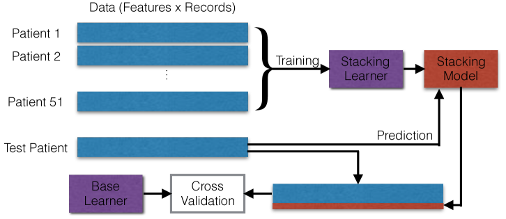
Fig 12: How we Implement Stacking.

This stacking approach is motivated by the realization that, as our data is self-reported, some patients (such as patient 16) have a large number of records, while other patients have relatively few records. Consider the datasets (features and outcome) for two patients, $D_{1}=\{(\mathbf{x}^{1}_{i},y^{1}_{i})|i=1..n\}$ and $D_{2}=\{(\mathbf{x}^{2}_{j},y^{2}_{j})|j=1..m\}$ where $m\ll n$. Let $f_{1}:\mathbf{X}\rightarrow Y$ and $f_{2}:\mathbf{X}\rightarrow Y$ be the true underlying glucose functions for these patients. Both functions are sufficiently complex that a learning algorithm cannot learn a good approximation $\hat{f}_{2}$ when only learning with $D_{2}$, but a learning algorithm can learn a good approximation $\hat{f}_{1}$ when only learning with $D_{1}$. If $f_{1}$ and $f_{2}$ are closely related in some sense – e.g., affinely related $f_{2}(\mathbf{x})=a\,f_{1}(\mathbf{x})+b$ – then $\hat{f}_{2}$ can be learned using $D_{1}$ and $D_{2}$ by first learning $\hat{f}_{1}$. As another perspective, we could view this stacking approach as mimicking health care professionals, who apply the knowledge that they have acquired from previous patients, to a new patient.

Competing interests

The authors declare that they have no competing interests.

Author’s contributions

Conceptualization:	NCB EAR RG
Data curation:	NCB EAR RG
Formal analysis:	NCB
Funding acquisition:	RG
Investigation:	NCB
Methodology:	NCB EAR RG
Project administration:	EAR RG
Resources:	EAR RG
Software:	NCB
Supervision:	EAR RG
Validation:	NCB EAR
Visualization:	NCB RG
Writing - original draft:	NCB EAR RG
Writing - review and editing:	NCB EAR RG

References

- 1. Daneman D. Type 1 diabetes. The Lancet. 2006;367(9513):847–858.
- 2. Kok P. Predicting blood glucose levels of diabetics using artificial neural networks. Research Assignment for Master of Science, Delft University of Technology. 2004;.
- 3. Bastani M. Model-free intelligent diabetes management using machine learning. Department of Computing Science, University of Alberta; 2014.
- 4. Lunze K, Singh T, Walter M, Brendel MD, Leonhardt S. Blood glucose control algorithms for type 1 diabetic patients: A methodological review. Biomedical Signal Processing and Control. 2013;8(2):107–119.
- 5. Tresp V, Briegel T, Moody J. Neural-network models for the blood glucose metabolism of a diabetic. IEEE Transactions on Neural networks. 1999;10(5):1204–1213.
- 6. Baghdadi G, Nasrabadi AM. Controlling blood glucose levels in diabetics by neural network predictor. In: Engineering in Medicine and Biology Society, 2007. EMBS 2007. 29th Annual International Conference of the IEEE. IEEE; 2007. p. 3216–3219.
- 7. Zainuddin Z, Pauline O, Ardil C. A neural network approach in predicting the blood glucose level for diabetic patients. International Journal of Computational Intelligence. 2009;5:72–79.
- 8. Georga EI, Protopappas VC, Polyzos D, Fotiadis DI. Online prediction of glucose concentration in type 1 diabetes using extreme learning machines. In: Engineering in Medicine and Biology Society (EMBC), 2015 37th Annual International Conference of the IEEE. IEEE; 2015. p. 3262–3265.
- 9. Andreassen S, Benn JJ, Hovorka R, Olesen KG, Carson ER. A probabilistic approach to glucose prediction and insulin dose adjustment: description of metabolic model and pilot evaluation study. Computer methods and programs in biomedicine. 1994;41(3-4):153–165.
- 10. Magni P, Bellazzi R. A stochastic model to assess the variability of blood glucose time series in diabetic patients self-monitoring. IEEE Transactions on biomedical engineering. 2006;53(6):977–985.
- 11. Gadaleta M, Facchinetti A, Grisan E, Rossi M. Prediction of Adverse Glycemic Events from Continuous Glucose Monitoring Signal. IEEE journal of biomedical and health informatics. 2018;.
- 12. Quinn CC, Shardell MD, Terrin ML, Barr EA, Ballew SH, Gruber-Baldini AL. Cluster-randomized trial of a mobile phone personalized behavioral intervention for blood glucose control. Diabetes care. 2011;34(9):1934–1942.
- 13. Chemlal S, Colberg S, Satin-Smith M, Gyuricsko E, Hubbard T, Scerbo MW, et al. Blood glucose individualized prediction for type 2 diabetes using iPhone application. In: Bioengineering Conference (NEBEC), 2011 IEEE 37th Annual Northeast. IEEE; 2011. p. 1–2.
- 14. Sudharsan B, Peeples M, Shomali M. Hypoglycemia prediction using machine learning models for patients with type 2 diabetes. Journal of diabetes science and technology. 2014;9(1):86–90.
- 15. Bunescu R, Struble N, Marling C, Shubrook J, Schwartz F. Blood glucose level prediction using physiological models and support vector regression. In: Machine Learning and Applications (ICMLA), 2013 12th International Conference on. vol. 1. IEEE; 2013. p. 135–140.
- 16. Eren-Oruklu M, Cinar A, Quinn L. Hypoglycemia prediction with subject-specific recursive time-series models; 2010.
- 17. Pappada SM, Cameron BD, Rosman PM, Bourey RE, Papadimos TJ, Olorunto W, et al. Neural network-based real-time prediction of glucose in patients with insulin-dependent diabetes. Diabetes technology & therapeutics. 2011;13(2):135–141.
- 18. Plis K, Bunescu R, Marling C, Shubrook J, Schwartz F. A machine learning approach to predicting blood glucose levels for diabetes management. Modern Artificial Intelligence for Health Analytics Papers from the AAAI-14. 2014;.
- 19. Contreras I, Vehi J. Artificial Intelligence for Diabetes Management and Decision Support: Literature Review. Journal of medical Internet research. 2018;20(5).
- 20. Pappada SM, Cameron BD, Rosman PM. Development of a neural network for prediction of glucose concentration in type 1 diabetes patients. Journal of diabetes science and technology. 2008;2(5):792–801.
- 21. Valletta JJ, Chipperfield AJ, Byrne CD. Gaussian process modelling of blood glucose response to free-living physical activity data in people with type 1 diabetes. In: Engineering in Medicine and Biology Society, 2009. EMBC 2009. Annual International Conference of the IEEE. IEEE; 2009. p. 4913–4916.
- 22. Duke DL. Intelligent diabetes assistant: A telemedicine system for modeling and managing blood glucose. Carnegie Mellon University; 2010.
- 23. Del Favero S, Facchinetti A, Cobelli C. A glucose-specific metric to assess predictors and identify models. IEEE Transactions on Biomedical Engineering. 2012;59(5):1281–1290.
- 24. Clarke WL. The original Clarke error grid analysis (EGA). Diabetes technology & therapeutics. 2005;7(5):776–779.
- 25. Borle N. The Challenge of Predicting Future Blood Glucose for Patients with Type I Diabetes. Department of Computing Science, University of Alberta; 2017.
- 26. Ryan EA, Holland J, Stroulia E, Bazelli B, Babwik SA, Li H, et al. Improved A1C Levels in Type 1 Diabetes with Smartphone App Use. Canadian Journal of Diabetes. 2017;41(1):33–40.
- 27. Al-Taee AM, Al-Taee MA, Al-Nuaimy W, Muhsin ZJ, AlZu’bi H. Smart bolus estimation taking into account the amount of insulin on board. In: Computer and Information Technology; Ubiquitous Computing and Communications; Dependable, Autonomic and Secure Computing; Pervasive Intelligence and Computing (CIT/IUCC/DASC/PICOM), 2015 IEEE International Conference on. IEEE; 2015. p. 1051–1056.
- 28. Mudaliar SR, Lindberg FA, Joyce M, Beerdsen P, Strange P, Lin A, et al. Insulin aspart (B28 asp-insulin): a fast-acting analog of human insulin: absorption kinetics and action profile compared with regular human insulin in healthy nondiabetic subjects. Diabetes care. 1999;22(9):1501–1506.
- 29. Gerich JE. Glucose counterregulation and its impact on diabetes mellitus. Diabetes. 1988;37(12):1608–1617.
- 30. Pedregosa F, Varoquaux G, Gramfort A, Michel V, Thirion B, Grisel O, et al. Scikit-learn: Machine Learning in Python. Journal of Machine Learning Research. 2011;12:2825–2830.
- 31. Chollet F, et al.. Keras; 2015. https://github.com/fchollet/keras.
- 32. Koivisto VA, Felig P, et al. Alterations in insulin absorption and in blood glucose control associated with varying insulin injection sites in diabetic patients. Ann Intern Med. 1980;92(1):59–61.
- 33. Unger RH, Cherrington AD. Glucagonocentric restructuring of diabetes: a pathophysiologic and therapeutic makeover. The Journal of clinical investigation. 2012;122(1):4.
- 34. Paterson M, Smart C, Lopez P, Howley P, McElduff P, Attia J, et al. Increasing the protein quantity in a meal results in dose-dependent effects on postprandial glucose levels in individuals with Type 1 diabetes mellitus. Diabetic Medicine. 2017;34(6):851–854.
- 35. Wolpert DH. Stacked generalization. Neural networks. 1992;5(2):241–259.
- 36. Marton ZC, Seidel F, Balint-Benczedi F, Beetz M. Ensembles of strong learners for multi-cue classification. Pattern Recognition Letters. 2013;34(7):754–761.