User Preference Aware Lossless Data Compression at the Edge

Abstract

Data compression is an efficient technique to save data storage and transmission costs. However, traditional data compression methods always ignore the impact of user preferences on the statistical distributions of symbols transmitted over the links. Notice that the development of big data technologies and popularization of smart devices enable analyses on user preferences based on data collected from personal handsets. This paper presents a user preference aware lossless data compression method, termed edge source coding, to compress data at the network edge. An optimization problem is formulated to minimize the expected number of bits needed to represent a requested content item in edge source coding. For edge source coding under discrete user preferences, DCA (difference of convex functions programming algorithm) based and $k$-means++ based algorithms are proposed to give codebook designs. For edge source coding under continuous user preferences, a sampling method is applied to give codebook designs. In addition, edge source coding is extended to the two-user case and codebooks are elaborately designed to utilize multicasting opportunities. Both theoretical analysis and simulations demonstrate the optimal codebook design should take into account user preferences.

I Introduction

With the popularization of smart devices and the rise of mobile multimedia applications, network traffic has undergone an explosive growth in the past decades. By using fewer bits to encode information than the original representation, data compression is an efficient technique to reduce the cost of storing or transmitting data. Traditional data compression methods are always source-based. The major design criterion is the average compression ratio for content generated by the information source. In the era of 5G, a large number of various content items are generated at the network. Because each user might only be interested in a few kinds of content items, a source-based data compression algorithm probably cannot achieve a satisfactory compression ratio for these specific kinds of content items. Recently the development of big data technologies and popularization of smart devices enable us to analyze user preferences and predict user requests based on private data collected from personal handsets. It becomes possible to improve the efficiency of data compression according to user preferences.

Since C. E. Shannon published his famous source coding theorem [1], data compression has been widely studied and various data compression schemes have been proposed. The LZ77 algorithm was presented in [2], which is the basis of several ubiquitous compression schemes, including ZIP and GIF. To improve the compression ratio, lossy compression algorithms for various types of content have also been developed, such as MPEG-4 for videos [3] and JPEG for images [4]. To solve the scalability problem resulting from packet classification in network services, a lossy compression based classifier was designed to reduce the classifier size [5]. Recently considerable attention has been paid to data compression in sensor networks [6]-[8]. A lossy compression algorithm was proposed to cope with large volumes of data generated by meters in smart distribution systems [6]. To reduce the power consumption of wireless sensors in Internet of Things applications, [7] proposed a hybrid data compression scheme, in which both lossless and lossy techniques were used. For wireless sensor networks with correlated sparse sources, a complexity-constrained distributed variable-rate quantized compression sensing method was developed in [8]. Machine learning techniques were also applied in data compression and transmission [9]-[10]. A joint source-channel coding design of text was provided by deep learning in [9]. End-to-end communications were implemented by neural networks in [10].

With the coming of Internet of Things and 5G, the edge of networks is attracting more and more attentions [11], because it can handle the concerns of latency requirement, bandwidth saving, and data security [12]. Edge computing has the potential to support “smart city” [13], improve vehicle services [14], and implement task offloading [15]. As edge nodes are closer to users, caching in the edge is capable of reducing the delivery latency and network congestion. Various content delivery and caching schemes were developed for edge networks [16]-[22]. The energy efficiency of edge caching was revealed in [19]. In [20], a learning-based method was proposed for edge caching. Furthermore, many papers have focused on improve the performance of edge caching via user preferences [23]-[26]. In edge networks, user preferences also contribute to improve streaming video services [27], the Quality-of-Experience [28], wireless resource allocations [29], and device-to-device content deliveries [30].

In this paper, we are interested in data compression at the edge under user preferences. More specifically, we consider the situation in which users are located at the network edge and are connected to content providers through a service provider. In traditional communication systems, data compression processes are executed at content providers when content items are generated. In these compression processes, more common symbols should be assigned with shorter codewords to minimize the expected codeword length according to information theory [31]. However, because user interests vary with content items, a symbol that is common in the whole set of content items might not be common in the requested content items. In other words, the statistical distribution of symbols in the transmission link is not likely to be identical to that in the information source due to user preferences. As a result, it is necessary to re-compress content items at the service provider according to user preferences. In this paper, a user preference aware lossless data compression scheme, termed edge source coding, is proposed to compress data according to finitely many codebooks at the network edge.

To obtain the optimal codebooks, we formulate an optimization problem for edge source coding, which is however nonconvex for the general case. For edge source coding with a single codebook, we solve the optimization problem via the method of Lagrange multipliers. An optimality condition is further presented. For edge source coding under discrete user preferences, the optimization problem reduces to a clustering problem. DCA (difference of convex functions programming algorithm) based and $k$-means++ based algorithms are proposed to give codebook designs [32]. For edge source coding under continuous user preferences, a sampling based method is applied to give codebook designs. We further extend edge source coding to the two-user case and present two algorithms to reduce transmission costs by using multicasting opportunities. Finally, simulation results are presented to demonstrate the potential of edge source coding and the performance of our algorithms.

The rest of the paper is organized as follows. Section II presents the content distribution system model and the concept of edge source coding. And then the formulation of edge source coding is given in Section III. Sections IV presents codebook designs for edge source coding. In Section V, edge source coding for two users with preference correlation is studied. Simulation results are presented in Section VI. Finally, Section VII concludes this paper and lists some directions for future research.

II System Model

In this section, we present our system model, based on which the key idea of edge source coding is introduced.

II-A Content Distribution System

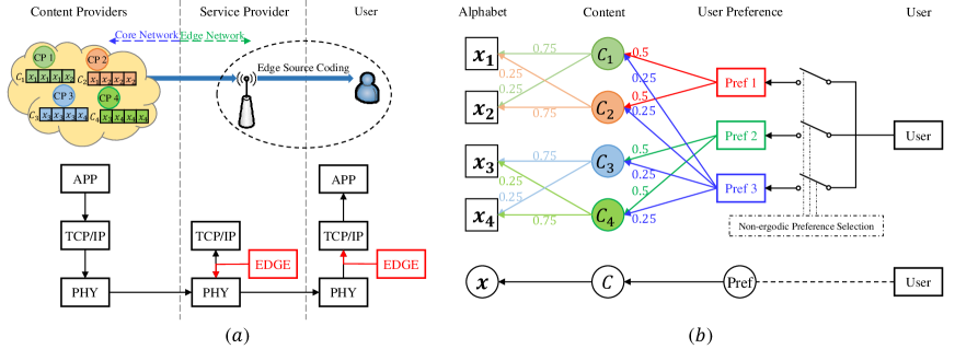
Figure 1: Content distribution system and a demo to illustrate how user preferences impact the statistical distributions of symbols transmitted in the network edge. In this realization, the alphabet is $\mathcal{X}=\{x_{1},x_{2},x_{3},x_{4}\}$. The four content items $C_{1}$, $C_{2}$, $C_{3}$, and $C_{4}$ generated by the four CPs are with SPVs $\bm{p}_{1}=[0.75,0.25,0,0],\bm{p}_{2}=[0.25,0.75,0,0],\bm{p}_{3}=[0,0,0.75,0.25],$ and $\bm{p}_{4}=[0,0,0.25,0.75]$, respectively. The user has three possible preferences. Under Pref 1, the symbols $x_{3}$ and $x_{4}$ never appear in the link from the service provider to the user.

Consider a content distribution system as shown in Fig. 1. A user is interested in content items generated by content providers (CPs) scattered around the Web. A base station (BS) serves as service provider to satisfy the user requests. Assume each CP produces its content item by choosing symbols from the same alphabet $\mathcal{X}=\{x_{1},...,x_{N}\}$ and each content item consists of $L$ symbols. The $L$ symbols of a content item are generated independently and based on the same discrete distribution, denoted by $\bm{p}=[p_{1},...,p_{N}]$, where $p_{n}$ denotes the probability that a symbol is $x_{n}$. The vector $\bm{p}$ is an attribute of that content item and will be referred to as the symbol probability vector (SPV). Note that a content item with SPV $\bm{p}$ has entropy $LH(\bm{p})=-L\sum_{n=1}^{N}p_{n}\log p_{n}$. All the feasible SPVs form a set $\Omega=\large\{[p_{1},...,p_{N}]:\sum_{n=1}^{N}p_{n}=1\text{ and }p_{n}\geq 0\text{ for }n\in[N]\}$.

In the content distribution system, the user issues requests for the content items. Let $f(\bm{p})$ describe the interest of the user in the content item with SPV $\bm{p}$. Then $f$ is a probability density function with support set $\Omega$. The function $f$ will also be referred to as the user preference. To give further insights, we present a tripartite graph model as shown in Fig. 1$(b)$. As stated before, each content item has its own probability distribution of the symbols, i.e., SPV. The symbol distributions of two content items can be totally different. We assume that each user has an individual preference that can be characterized by the request probability for various content items. In practice, the empirical request probability can be learned from a user’s historical requests. Further, we assume that a user has a fixed preference in our considered timescale. In other words, a non-ergodic preference selection is assumed to determine the preference of a user newly accessing to the service provider, or more particularly, a BS. In other words, the random symbols of the equivalent source at the edge are generated according to a simple probabilistic graphical model, as shown at the bottom of Fig. 1$(b)$.

The BS responds to a user request and initiates an end-to-end transmission to satisfy it. To improve transmission efficiency, data compression techniques can be used to eliminate statistical redundancy of the original symbol sequences. Traditionally, data compression is executed only in application (APP) layers at the content providers. Content items are compressed according to the statistical distributions of symbols, i.e., their SPVs, and are associated with codebooks for decoding. Edge information including user preferences is always ignored in traditional data compression methods, which however have a significant impact on the statistical distributions of symbols transmitted at the edge, as illustrated in Fig. 1. To reduce the transmission cost at the network edge, we present a user preference aware lossless data compression method, termed edge source coding, to re-compress original symbol sequences at the service provider. As shown in Fig. 1$(a)$, edge source coding exploits edge information in physical (PHY) layer transmissions.

II-B Edge Source Coding

In edge source coding, the BS compresses the content items according to finitely many binary codebooks to satisfy the user requests. These binary codebooks are cached in both the BS and the user. In this way, the encoded symbol sequences do not need to be associated with a whole codebook for decoding. Let $K$ be the total number of codebooks used in edge source coding. In the $k$-th codebook, the symbol $x_{n}$ is represented by $l_{k,n}$ bits. If the BS applies the $k$-th codebook to encode a content item with SPV $\bm{p}$, this content item can be represented by $L\sum_{n=1}^{N}p_{n}l_{k,n}=L(H(\bm{p})+D(\bm{p}||\bm{q_{k}}))$ bits, where $\bm{q}_{k}=[q_{k,1},...,q_{k,n}]$ and $q_{k,n}=2^{-l_{k,n}}$. To satisfy the request for this content item, the BS only needs to transmit these $L\sum_{n=1}^{N}p_{n}l_{k,n}$ bits. The user can decode the received bits by trying all the cached codebooks. In the rest of this paper, we also use $\bm{q}_{k}$ to represent the $k$-th codebook. According to Kraft’s inequality [31], $\bm{q}_{k}$ should satisfy

$$\sum_{n=1}^{N}q_{k,n}\leq 1$$ (1)

to ensure decodability.

As there are $K$ codebooks, the minimum cost to satisfy a request for the content item with SPV $\bm{p}$ is given by $L(H(\bm{p})+\min_{k\in[K]}D(\bm{p}||\bm{q_{k}}))$. Because the SPV of the requested content item obeys a probability density function $f$, the transmission cost for a requested content item is given by

$$\begin{split}\int_{\bm{p}\in\Omega}f(\bm{p})\left(L\left(H(\bm{p})+\min_{k\in[K]}D(\bm{p}||\bm{q_{k}})\right)\right)d\bm{p}.\end{split}$$ (2)

In this paper, we aim to design codebooks to minimize the transmission cost, i.e., expected number of bits to represent a requested content item.

III User Preference Aware Compression: A Problem Formulation

In this section, we formulate an optimization problem for edge source coding and solve it for the $K=1$ case. In addition, an optimality condition for the optimization problem is presented.

As stated in Subsection II-B, the codebooks can be described by $\{\bm{q}_{k}:k\in[K]\}$. Kraft’s inequality is a sufficient and necessary condition for the existence of a uniquely decodable code. We only require $\bm{q}_{k}$ to obey Kraft’s inequality and relax the constraint that each component of $\bm{q}_{k}$ should be a negative integer power of two. Note that Eq. (2) can be rewritten as

$$\begin{split}L\int_{\bm{p}\in\Omega}f(\bm{p})H(\bm{p})d\bm{p}+L\int_{\bm{p}\in\Omega}f(\bm{p})\min_{k\in[K]}D(\bm{p}||\bm{q_{k}})d\bm{p}\end{split}$$ (3)

To minimize the transmission cost, we only need to minimize $\int_{\bm{p}\in\Omega}f(\bm{p})\min_{k\in[K]}D(\bm{p}||\bm{q_{k}})d\bm{p}$ in Eq. (3), which indicates the additional transmission cost per symbol under user preference $f$ due to the mismatch between SPVs and codebooks.

Let $\Omega_{k}$ be the set of SPVs that have the smallest Kullback-Leibler divergence with codebook $\bm{q}_{k}$ among all the codebooks, i.e.,

$$\Omega_{k}=\{\bm{p}:\bm{p}\in\Omega,D(\bm{p}||\bm{q_{k}})\leq D(\bm{p}||\bm{q_{j}})\text{ for }j\in[K]\}.$$ (4)

One can see that the sets $\Omega_{k}$ are disjoint, $\Omega=\cup_{k=1}^{K}\Omega_{k}$, and $\min_{j\in[K]}D(\bm{p}||\bm{q}_{j})=D(\bm{p}||\bm{q}_{k})$ for $\bm{p}\in\Omega_{k}$. To minimize the transmission cost per symbol, a content item with SPV belonging to $\Omega_{k}$ should be encoded according to codebook $\bm{q_{k}}$. The following optimization problem gives the optimal codebook design:

$$\begin{split}\min_{\bm{q}_{k}}\quad&\sum_{k=1}^{K}\int_{\bm{p}\in\Omega_{k}}f(\bm{p})D(\bm{p}||\bm{q}_{k})d\bm{p}\\ \text{s.t.}\quad&\text{Eqs. }(\ref{kraft})\text{ and }(\ref{split_omega}),\\ &q_{k,n}\geq 0,k\in[K],n\in[N].\end{split}$$ (5)

In the objective function, the integral over $\Omega$ is calculated by summing up the integrals over its subsets $\Omega_{k}$. Note that swapping the values of different $\bm{q}_{k}$ does not change the objective value of problem (5). Thus, problem (5) has more than one optimal solutions, which further implies the nonconvexity of problem (5).

Because $\Omega_{k}$ is a set depending on ${\bm{q}_{k}},$ it is nontrivial to solve problem (5) for the general case. We first solve problem (5) for $K=1$ to give greater insight. In this case, there is only one codebook $\bm{q}_{1}$ and thus we denote it as $\bm{q}=[q_{1},...,q_{n}]$ for simplicity. Theorem 1 presents the optimal codebook design.

Theorem 1.

For $K=1$, the optimal codebook for edge source coding is given by

$$q_{n}=\frac{\mathbb{E}\{p_{n}\}}{\sum_{j=1}^{N}\mathbb{E}\{p_{j}\}}.$$ (6)

Proof.

Let us consider the Lagrange function

$$L(\bm{q},\lambda)=\int_{\bm{p}\in\Omega}f(\bm{p})D(\bm{p}||\bm{q})d\bm{p}+\lambda(\bm{1}^{T}\bm{q}-1),$$ (7)

where $\lambda$ is the Lagrange multiplier and $\bm{1}$ is an $N$-dimensional vector all of whose components are equal to 1. The partial derivative of $L(\bm{q},\lambda)$ with respect to $q_{n}$ is given by

$$\begin{split}\frac{\partial L(\bm{q},\lambda)}{\partial q_{n}}&=-\frac{1}{q_{n}}\int_{\bm{p}\in\Omega}f(\bm{p})p_{n}d\bm{p}+\lambda\\ &=\lambda-\frac{\mathbbm{E}\{p_{n}\}}{q_{n}}.\end{split}$$ (8)

By the optimality conditions $\frac{\partial L(\bm{q},\lambda)}{\partial q_{n}}=0$ and $\bm{1}^{T}\bm{q}=1$, the optimal codebook can be derived as Eq. (6). ∎

In the optimal codebook, the codeword of $x_{n}$ consists of $-\log q_{n}$ bits. Eq. (6) implies that the more frequently the requested content items contain a symbol, the shorter the codeword corresponding to this symbol will be. To improve the data compression efficiency at the network edge, user preferences must be taken into account in designing the codebook.

Based on Theorem 1, the following theorem gives an optimality condition for any values of the number of codebooks, i.e., $K$.

Theorem 2.

The optimal codebook design for edge source coding satisfies

$$q_{k,n}=\frac{\mathbb{E}\{p_{n}|\bm{p}\in\Omega_{k}\}}{\sum_{j=1}^{N}\mathbb{E}\{p_{j}|\bm{p}\in\Omega_{k}\}},$$ (9)

where $\Omega_{k}$ is defined in Eq. (4).

Proof.

After splitting $\Omega$ into $K$ disjoint subsets $\Omega_{k}$, the codebook $\bm{q}_{k}$ is used to encode content items with SPV in $\Omega_{k}$. Applying Theorem 1 on each set $\Omega_{k}$ yields Eq. (9). ∎

Theorem 2 reveals the coupling between the optimal $\bm{q}_{k}$ and $\Omega_{k}$. Note that the inequality $D(\bm{p}||\bm{q_{k}})\leq D(\bm{p}||\bm{q_{j}})$ can be expanded as

$$\sum_{n=1}^{N}p_{n}\log\frac{q_{j,n}}{q_{k,n}}\leq 0$$ (10)

which is a linear inequality in the vector $\bm{p}$. Then $\Omega_{k}$ is a convex polytope characterized by hyperplanes defined by $\{\bm{q}_{k}:k\in[K]\}$. The vector $\bm{q}_{k}$ can be given by conditional expectations over $\Omega_{k}.$ To some extend, $\bm{q}_{k}$ can be viewed as a central point in $\Omega_{k}$.

IV Codebook Design for User Preference Aware Compression

In this section, we investigate codebook design for edge source coding under user preference $f$. If the user is interested only in finitely many content items, $f$ reduces to a probability mass function. Then $f$ is referred to as a discrete user preference. If $f$ is a continuous probability density function over $\Omega$, $f$ is referred to as a continuous user preference. Codebook designs for both discrete and continuous user preferences are considered in this section. It will be shown that codebook designs rely on user preferences in both the two cases.

IV-A DCA based Codebook Design under Discrete User Preferences

In this subsection, edge source coding under discrete user preferences is studied. Mathematically, $f(\bm{p})$ is nonzero only at finite points. As a result, the edge source coding problem becomes a clustering problem. A DCA (difference of convex functions programming algorithm) based algorithm is proposed to give a codebook design.

Denote the set of nonzero points of $f$ as $\Omega^{d}=\{\bm{p}_{1},...,\bm{p}_{J}\}$. We have $\Omega^{d}\subseteq\Omega$ and $|\Omega^{d}|=J$. Let $f_{j}$ be the probability that the content item with SPV $\bm{p}_{j}$ is requested. Then, we have $f_{j}=f(\bm{p}_{j})$ and $\sum_{j=1}^{J}f_{j}=1$. In this case, problem (5) becomes the following form:

$$\begin{split}\min_{\bm{q}_{k}}\quad&\sum_{k=1}^{K}\sum_{j\in\Omega_{k}^{d}}f_{j}D(\bm{p}_{j}||\bm{q}_{k})\\ \text{s.t.}\quad&\bm{1}^{T}\bm{q}_{k}\leq 1,k\in[K],\hskip 65.72578pt(\ref{op_2}.a)\\ &q_{k,n}\geq 0,k\in[K],n\in[N],\hskip 28.45274pt(\ref{op_2}.b)\end{split}$$ (11)

where

$$\Omega_{k}^{d}=\{j:D(\bm{p}_{j}||\bm{q}_{k})\leq D(\bm{p}_{j}||\bm{q}_{i})\text{ for }i\in[K]\}.$$ (12)

Similarly, a content item with SPV in $\Omega_{k}^{d}$ should be encoded by codebook $\bm{q}_{k}$ in order to minimize the transmission cost.

Problem (11) can be viewed as a clustering problem. The $J$ points in $\Omega^{d}$ are clustered into $K$ subsets. In the discrete case, Eq. (9) becomes

$$q_{k,n}=\frac{\sum_{j\in\Omega_{k}^{d}}f_{j}p_{j,n}}{\sum_{i=1}^{N}\sum_{j\in\Omega_{k}^{d}}f_{j}p_{j,i}}.$$ (13)

Again, Eq. (13) implies that the best codebook design should take into account the discrete user preferences. Once the optimal clustering scheme is obtained, the optimal codebooks can be derived from Eq. (13). To solve problem (11) is to find the optimal clustering scheme. However, there are around $K^{J}$ clustering schemes. It is computationally prohibitive to traverse all the possible ones. To give a suboptimal clustering scheme within affordable space and time costs, we transform problem (11) into a DC (difference of convex functions) programming problem and present a DCA based method to give an appropriate clustering scheme. The core idea behind the construction of the DC programming is probabilistic clustering in which the codebook used to encode each content item is randomly selected.

Lemma 1 presents an equivalent problem for problem (11) in which the variables $\Omega_{k}$ are removed.

Lemma 1.

Problem (11) is equivalent to the following problem:

$$\begin{split}\min_{r_{j,k}}\quad&\sum_{k=1}^{K}\sum_{j=1}^{J}\sum_{n=1}^{N}f_{j}p_{j,n}r_{j,k}\log\frac{\sum_{j=1}^{J}\sum_{i=1}^{N}f_{j}p_{j,i}r_{j,k}}{\sum_{j=1}^{J}f_{j}p_{j,n}r_{j,k}}\\ \text{s.t.}\quad&\sum_{k=1}^{K}r_{j,k}=1,j\in[J],\hskip 56.9055pt(\ref{op_4}.a)\\ &r_{j,k}\geq 0,k=\in[K],j\in[J].\hskip 28.45274pt(\ref{op_4}.b)\end{split}$$ (14)

Proof.

The key to prove the equivalence between two optimization problems is to show that the optimal solution of one can be easily derived from the optimal solution of the other and vice-versa. We first show the transformation from the optimal solution of problem (11) to that of problem (14). Let us consider a probabilistic clustering scheme. For the content item with SPV $\bm{p}_{j}$, let $r_{j,k}$ be the probability that codebook $q_{k}$ is selected to encode it. Then problem (11) can be rewritten as

$$\begin{split}\min_{\bm{q}_{k},r_{j,k}}\quad&\sum_{j=1}^{J}\sum_{k=1}^{K}f_{j}r_{j,k}D(\bm{p}_{j}||\bm{q}_{k})\\ \text{s.t.}\quad&\bm{1}^{T}\bm{q}_{k}\leq 1,k\in[K],\hskip 126.04549pt(\ref{op_3}.a)\\ &\sum_{k=1}^{K}r_{j,k}=1,j\in[J],\hskip 117.79439pt(\ref{op_3}.b)\\ &q_{k,n},r_{j,k}\geq 0,k\in[K],n\in[N],j\in[J],\hskip 28.45274pt(\ref{op_3}.c)\end{split}$$ (15)

where the constraint Eq. ($\ref{op_3}.b$) corresponds to the probability normalization.

The method of Lagrange multipliers can be used to simplify problem (15). Let us consider the Lagrange function

$$L(\bm{q}_{k},r_{j,k},\lambda_{k},\mu_{j})=\sum_{j=1}^{J}\sum_{k=1}^{K}f_{j}r_{j,k}D(\bm{p}_{j}||\bm{q}_{k})+\sum_{k=1}^{K}\lambda_{k}(\bm{1}^{T}\bm{q}_{k}-1)+\sum_{j=1}^{J}\mu_{j}\left(\sum_{k=1}^{K}r_{j,k}-1\right).$$ (16)

The partial derivative of $L(\bm{q}_{k},r_{j,k},\lambda_{k},\mu_{j})$ with respect to $q_{k,n}$ is given by

$$\begin{split}\frac{\partial L(\bm{q}_{k},r_{j,k},\lambda_{k},\mu_{j})}{\partial q_{k,n}}&=-\frac{1}{q_{k,n}}\sum_{j=1}^{J}f_{j}p_{j,n}r_{j,k}+\lambda_{k}.\end{split}$$ (17)

Again, we have

$$q_{k,n}=\frac{\sum_{j=1}^{J}f_{j}p_{j,n}r_{j,k}}{\sum_{j=1}^{J}\sum_{i=1}^{N}f_{j}p_{j,i}r_{j,k}}.$$ (18)

according to the optimality conditions $\frac{\partial L(\bm{q}_{k},r_{j,k},\lambda_{k},\mu_{j})}{\partial q_{k,n}}=0$ and $\sum_{n=1}^{N}q_{k,n}=1$. It can be seen that Eqs. (18) and (13) are very similar. If we impose each $r_{j,k}$ equal to 0 or 1, Eq. (18) reduces to Eq. (13). That is because the deterministic clustering is a special case of probabilistic clustering. Substituting Eq. (18) into problem (15) yields problem (14).

Suppose $\{\bm{q}_{k}^{*}:k\in[K]\}$ is the optimal solution of problem (11). We set

$$r_{j,k}^{*}=\begin{cases}1,&\text{if }k=\arg\min_{k_{0}\in[K]}D(\bm{p}_{j}||\bm{q}_{k_{0}}^{*}),\\ 0,&\text{if }k\neq\arg\min_{k_{0}\in[K]}D(\bm{p}_{j}||\bm{q}_{k_{0}}^{*}).\end{cases}$$ (19)

Then $\{\bm{q}_{k}^{*}\}$ and $\{r_{j,k}^{*}\}$ form the optimal solution of problem (15) and Eq. (18) holds for $\{\bm{q}_{k}^{*}\}$ and $\{r_{j,k}^{*}\}$. As a result, $\{r_{j,k}^{*}\}$ is the optimal solution of problem (14). The transformation from from the optimal solution of problem (14) to that of problem (11) is presented in Appendix. ∎

Note that $r_{j,k}$ represents that the probability that the content item with SPV $\bm{p}_{j}$ is encoded by codebook $\bm{q}_{k}$. Lemma 1 indicates the best probabilistic clustering is exactly a deterministic clustering. Although the constraints of problem (14) are linear, problem (14) is still intractable due to the nonconvex objective function. Notice the objective function of problem (14) contains the logarithms of fractions. We can transform the original problem (11) into a DC programming problem and apply DCA to solve it.

Theorem 3.

Problem (11) is equivalent to a DC programming problem having the following form:

$$\begin{split}\min_{\bm{x}}\quad&\sum_{m=1}^{M}\lambda_{1,m}x_{m}\log x_{m}-\sum_{m=1}^{M}\lambda_{2,m}x_{m}\log x_{m}\\ \text{s.t.}\quad&\bm{A}_{1}\bm{x}=\bm{b}_{1},\hskip 63.5064pt(\ref{op_5}.a)\\ &x_{m}\geq 0,m\in[M],\hskip 28.45274pt(\ref{op_5}.b)\end{split}$$ (20)

where $M=K+KN+KJ$, $\lambda_{1,m}=1$ for $1\leq m\leq M$, $\lambda_{1,m}=0$ for other values of $m$, $\lambda_{2,m}=1$ for $K+1\leq m\leq K+KN$, and $\lambda_{2,m}=0$ for other values of $m$.

Proof.

According to Lemma 1, we only need to show the equivalence between problems (14) and (20). By introducing two groups of auxiliary variables

$$s_{k,n}=\sum_{j=1}^{J}f_{j}p_{j,n}r_{j,k},\hskip 25.6073pt$$ (21)

$$t_{k}=\sum_{j=1}^{J}\sum_{i=1}^{N}f_{j}p_{j,i}r_{j,k},$$ (22)

and defining $\bm{x}=[t_{1},..,t_{K},s_{1,1},...,s_{K,N},r_{1,1},...,r_{J,K}]$, problem (14) can be rewritten (20). ∎

Algorithm 1 DCA based Codebook Design under Discrete User Preferences

0:  $\bm{p}_{1},...,\bm{p_{J}},f_{1},...,f_{J},\varepsilon$;

0:  $\bm{q}_{1},...,\bm{q}_{K}$;

1:  Calculate $\bm{\lambda}_{1},\bm{\lambda}_{2},\bm{A}_{1},\bm{b}_{1}$ according to $\bm{p}_{1},...,\bm{p}_{J}$ and $f_{1},...,f_{J}$;

2:  Solve problem (20) according to Algorithm 2 and obtain $\bm{x}^{\text{opt}}$;

3:  Extract $r_{1,1},...,r_{J,K}$ from $\bm{x}^{\text{opt}}$;

4:  for $j=1$ to $J$ do

5:     $k^{\max}=\arg\max_{k}r_{j,k}$;

6:     Set $r_{j,k^{\max}}=1$ and $r_{j,k}=0$ for $k\neq k^{\max}$;

7:  end for

8:  Compute $\bm{q}_{1},...,\bm{q}_{K}$ according to Eq. (18).

Algorithm 2 DCA for Problem (20)

0:  $\bm{\lambda}_{1},\bm{\lambda}_{2},\bm{A}_{1},\bm{b}_{1},\varepsilon$;

0:  $\bm{x}^{\text{opt}}$;

1:  Randomly initialize $\bm{x}^{\text{old}}$ satisfying $\bm{A}_{1}\bm{x}^{\text{old}}=\bm{b}_{1}$;

2:  Calculate $R^{\text{new}}=\sum_{m=1}^{M}(\lambda_{1,m}-\lambda_{2,m})x_{m}^{\text{old}}\log x_{m}^{\text{old}}$;

3:  Initialize $R^{\text{old}}=\inf$;

4:  while $|R^{\text{old}}-R^{\text{new}}|>\varepsilon$ do

5:     $R^{\text{old}}=R^{\text{new}}$;

6:     for $m=1$ to $M$ do

7:        $y_{m}^{\text{old}}=\lambda_{2,m}(1+\log(x_{m}^{\text{old}}))$;

8:     end for

9:     Solve problem (23) and obtain $\bm{x}^{\text{new}}$;

10:     Calculate $R^{\text{new}}=\sum_{m=1}^{M}(\lambda_{1,m}-\lambda_{2,m})x_{m}^{\text{new}}\log x_{m}^{\text{new}}$;

11:     $x^{\text{old}}=x^{\text{new}}$;

12:  end while

13:  $\bm{x}^{\text{opt}}=\bm{x}^{\text{new}}$.

Note that $s_{k,n}$ is weighted average of SPVs. The weights are related to the probabilities in the probabilistic clustering scheme. In problem (20), the linear equality constraint $\bm{A}_{1}\bm{x}=\bm{b}_{1}$ results from Eqs. ($\ref{op_4}.a$), (21), and (22). Denote $\bm{\lambda}_{1}=[\lambda_{1,1},...,\lambda_{1,M}]$ and $\bm{\lambda}_{2}=[\lambda_{2,1},...,\lambda_{2,M}]$, which are two 0-1 vectors. Algorithm 1 provides a codebook design based on DCA for problem (20). Considering Lemma 1 implies that each $r_{j,k}$ is 0-1 in the optimal solution, Algorithm 1 resets the values of $r_{j,k}$ in Steps 4-7 after obtaining $\bm{x}^{\text{opt}}$ from Algorithm 2. Algorithm 2 provides a suboptimal solution for problem (20) by solving the following convex problem iteratively:

$$\begin{split}\min_{\bm{x}}\quad&\sum_{m=1}^{M}\lambda_{1,m}x_{m}\log x_{m}-\left(\bm{y}^{\text{old}}\right)^{T}\bm{x}\\ \text{s.t.}\quad&\bm{A}_{1}\bm{x}=\bm{b}_{1},\hskip 62.0268pt(\ref{op_6}.a)\\ &x_{m}\geq 0,m\in[M].\hskip 28.45274pt(\ref{op_6}.b)\end{split}$$ (23)

In each iteration, $\bm{y}^{\text{old}}$ is calculated in Steps 6-8. It can be seen that $\bm{y}^{\text{old}}$ is the gradient of function $\sum_{m=1}^{M}\lambda_{2,m}x_{m}\log x_{m}$ at the point $\bm{x}^{\text{old}}$. Then $\left(\bm{y}^{\text{old}}\right)^{T}\bm{x}+C$ is a local approximation of function $\sum_{m=1}^{M}\lambda_{2,m}x_{m}\log x_{m}$ ($C$ is a constant). This is the reason we use $\left(\bm{y}^{\text{old}}\right)^{T}\bm{x}$ to replace $\sum_{m=1}^{M}\mu_{m}x_{m}\log x_{m}$ in problem (23). It should be pointed out that it is easy to initialize $\bm{x}^{\text{old}}$ satisfying $\bm{A}_{1}\bm{x}^{\text{old}}=\bm{b}_{1}$. We only need to initialize $r_{j,k}$ satisfying Eqs. ($\ref{op_4}.a$) and ($\ref{op_4}.b$) and then generate $s_{k,n}$ and $t_{k}$ according to Eqs. (21) and (22).

IV-B $k$-means++ based Codebook Design under Discrete User Preferences

Algorithm 3 $k$-means++ based Codebook Design under Discrete User Preferences

0:  $\bm{p}_{1},...,\bm{p_{J}},f_{1},...,f_{J}$;

0:  $\bm{q}_{1},...,\bm{q}_{K}$;

1:  Randomly select a vector from $\Omega^{d}$ as $\bm{q}_{1}$ where $\bm{p}_{j}$ is selected with probability $f_{j}$;

2:  for $k=2$ to $K$ do

3:     Compute $G_{j}=\min_{i<k}D(\bm{p}_{j}||\bm{q}_{i})$ for $j=1,...,J$;

4:     Randomly select a vector from $\Omega^{d}$ as $\bm{q}_{k}$ where $\bm{p}_{j}$ is selected with probability proportional to $f_{j}G_{j}^{2}$;

5:  end for

6:  Initialize $\Omega_{k}^{d}$ according to Eq. (12);

7:  while Eq. (13) is FALSE for some $n,k$ do

8:     Update $\bm{q}_{k}$ according to Eq. (13);

9:     Update $\Omega_{k}$ according to Eq. (12);

10:  end while

11:  return  $\{\bm{q}_{k}:k=1,...,K\}.$

Recall that the edge source coding problem reduces to a clustering problem under discrete user preferences. Considering that $k$-means++ is a typical heuristic algorithm for clustering problems [32], we present a codebook design for edge source coding under discrete user preferences based on the $k$-means++ approach in this subsection, as detailed in Algorithm 1. In Steps 1-5, each codebook is initialized according to the probabilities of the SPVs and the Kullback-Leibler divergence with codebooks having been determined. In Steps 6-10, a variant of the $k$-means approach is employed to update the clustering centers $\{\bm{q}_{k}:k\in[K]\}$. Compared with the traditional $k$-means++ approach, Algorithm 3 uses the Kullback-Leibler divergence instead of Euclidean distance to reassign the points into different clusters. In addition, the center of a cluster is derived from some conditional expectations in Algorithm 3, which is usually not the arithmetic mean of points in this cluster.

Algorithm 4 $k$-means++ based Codebook Design under Continuous User Preferences

0:  $f,\varepsilon$;

0:  $\bm{q}_{1},...,\bm{q}_{K}$;

1:  Randomly select a vector from $\Omega$ as $\bm{q}_{1}$ according to probability density function $f$;

2:  for $k=2$ to $K$ do

3:     $g(p)=\min_{i<k}D(\bm{p}||\bm{q}_{i})$;

4:     Randomly select a vector from $\Omega$ as $\bm{q}_{k}$ according to $\frac{fg^{2}}{\int_{\bm{p}\in\Omega}fg^{2}d\bm{p}}$;

5:  end for

6:  Initialize $\Omega_{k}$ according to Eq. (4);

7:  while $\min_{k,n}\left|q_{k,n}-\frac{\mathbb{E}\{p_{n}|\bm{p}\in\Omega_{k}\}}{\sum_{j=1}^{N}\mathbb{E}\{p_{j}|\bm{p}\in\Omega_{k}\}}\right|>\varepsilon$ do

8:     Update $\bm{q}_{k}$ according to Eq. (9);

9:     Update $\Omega_{k}$ according to Eq. (4);

10:  end while

11:  return  $\{\bm{q}_{k}:k\in[K]\}.$

IV-C $k$-means++ based Codebook Design under Continuous User Preferences

In this subsection, we extend the $k$-means++ based algorithm proposed in the previous subsection to the continuous user preferences. Based on the coupling relationship between $\Omega_{k}$ and $\bm{q}_{k}$ revealed in Eqs. (4) and (9), Algorithm 4 presents an iterative method to obtain a suboptimal solution of problem (5), which is a continuous version of Algorithm 3. In Algorithm 4, the codebooks are also initialized based on user preferences. The parameter $\varepsilon$ in Step 7 is a sufficiently small positive number. Instead of summation, Algorithm 4 calculates several integrals to update $\bm{q}_{k}$. The convergence of Algorithm 4 is guaranteed by the fact that each update of $\bm{q}_{k}$ or $\Omega_{k}$ achieves a lower objective value of problem (5). Thus, Algorithm 4 at least reaches a locally optimal point.

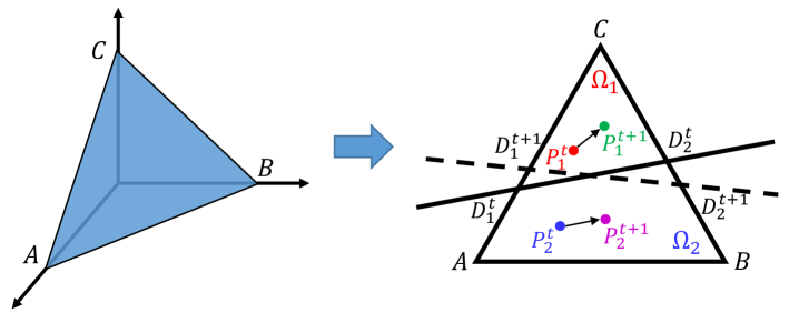
Figure 2: Illustration of the iterative process for $N=3$ and $K=2$.

We illustrate the iterative process in Algorithm 4 by the case $N=3$, $K=2$, and the user preferences are uniform, i.e., $f=1/\int_{\bm{p}\in\Omega}d\bm{p}$. In this case, the set $\Omega$ is formed by points in an equilateral triangle with vertices $A=[1,0,0],B=[0,1,0],$ and $C=[0,0,1]$, as shown in Fig. 2. The codebooks $\bm{q}_{1}$ and $\bm{q}_{2}$ are two three-dimensional vectors, corresponding to $P_{1}^{t}$ and $P_{2}^{t}$ respectively after the $t$-th iteration. Because there are only two codebooks, we need just a single hyperplane to split $\Omega$. The hyperplane is a line in the $N=3$ case, denoted as $D_{1}^{t}D_{2}^{t}$. Note that $D_{1}^{t}D_{2}^{t}$ is not the perpendicular bisector of $P_{1}^{t}P_{2}^{t}$ but instead is given by the equality $\sum_{n=1}^{3}p_{n}(\log q_{1,n}-\log q_{2,n})=0$. In the $(t+1)$-th iteration, the points corresponding to the two codebooks are updated to $P_{1}^{t+1}$ and $P_{2}^{t+1}$, which happen to be the centroids of the triangle $CD_{1}^{t}D_{2}^{t}$ and quadrilateral $AD_{1}^{t}D_{2}^{t}B$. When the user preferences are uniform, $P_{1}^{t+1}$ can be obtained by

$$P_{1}^{t+1} = \frac{C+D_{1}^{t}+D_{2}^{t}}{3}.$$ (24)

$P_{2}^{t+1}$ can also be obtained by a short calculation [33]. After obtaining $P_{1}^{t+1}$ and $P_{2}^{t+1}$, the new split line $D_{1}^{t+1}D_{2}^{t+1}$ can be calculated and further $\Omega_{1}$ and $\Omega_{2}$ are updated.

In the general case, namely, $f$ is an arbitrary probability density function and $N\geq 3$, it is intractable to calculate integrals over $\Omega_{k}$. This is because $\Omega_{k}$ is a convex polytope bounded by high dimensional hyperplanes. As a result, Algorithm 4 is of high computational complexity for arbitrary $f$ and large $N$. More specifically, the integrals over sets $\Omega_{k}$ induce the majority of the computational complexity. In the following subsection, we overcome this by a sampling method.

IV-D Sampling based Codebook Design under Continuous User Preferences

Algorithm 5 Sampling based Codebook Design under Continuous User Preferences

0:  $f,S$;

0:  $\bm{q}_{1},...,\bm{q}_{K}$;

1:  Sample $S$ points from $\Omega$ as $\bm{p}_{1},...,\bm{p}_{S}$ according to probability density function $f$;

2:  Set $f_{s}=\frac{1}{S}$ for $s=1,...,S;$

3:  Run Algorithm 3 or Algorithm 1 with $\bm{p}_{1},..,\bm{p}_{S},f_{1},...,f_{S}$ as input and obtain $\bm{q}_{1},...,\bm{q}_{K}$;

4:  return  $\{\bm{q}_{k}:k\in[K]\}.$

Algorithm 5 presents a sampling based method to give a codebook design for edge source coding under continuous user preferences. The core idea behind Algorithm 5 is that integrals over a set with a probability measure can be estimated by summations over sample points. In Algorithm 5, $S$ is the number of sample points. These points are sampled according to the function $f$. In Step 2, every sample point is associated with an identical probability $f_{s}=\frac{1}{S}$. Step 3 calls Algorithm 3 or Algorithm 1 to gives a suboptimal codebook design.

The number of sample points $S$ is a key parameter in Algorithm 5. On the one hand, too large $S$ will result in a high computing time. On the other hand, too small $S$ will reduce the estimation accuracy of the sampling method. There are two versions of Algorithm 5 according to the algorithm called in Step 3. Simulations will demonstrate that these two versions of Algorithm 5 have similar performance.

V Edge Source Coding for Two Users with Common Interests

In this section, we extend edge source coding to the two-user case, which will be referred to as user 1 and user 2. In contrast with the scenario considered in previous sections, two-user edge source coding is capable of reducing the total transmission cost by taking advantage of multicasting opportunities. The preferences of the two users will be described by a matrix.

Recall that $\Omega=\large\{[p_{1},...,p_{N}]:\sum_{n=1}^{N}p_{n}=1\text{ and }p_{n}\geq 0\text{ for }n=1,...,N\}$ represents the set of feasible SPVs. Let $\bm{p}[1]$ and $\bm{p}[2]$ denote the SPVs of the content items requested by user 1 and user 2, respectively. Then $\bm{p}[1]$ and $\bm{p}[2]$ are two random variables with support set $\Omega\times\Omega$. We denote the probability density function of $\bm{p}[1]$ and $\bm{p}[2]$ as $f(\bm{p}[1],\bm{p}[2])$. Let $K_{1}^{t}$ and $K_{2}^{t}$ be the total numbers of codebooks used by user 1 and user 2, respectively. As the two users probably request the same content item, we assume there are $K_{0}$ codebooks that the two users have in common, denoted by $\bm{q}_{1}^{0},...,\bm{q}_{K_{0}}^{0}$. In other words, user 1 and user 2 have $K_{1}=K_{1}^{t}-K_{0}$ and $K_{2}=K_{2}^{t}-K_{0}$ exclusive codebooks, respectively. Let $\{\bm{q}_{1}^{1},...,\bm{q}_{K_{1}}^{1}\}$ and $\{\bm{q}_{1}^{2},...,\bm{q}_{K_{2}}^{2}\}$ denote the sets of exclusive codebooks for user 1 and user 2, respectively.

In the two-user edge source coding, multicasting opportunities can be utilized when the two users request the same content item. In this case, the requested content item will be encoded by a common codebook of the $K_{0}$ ones and then be transmitted to the two users simultaneously. If the two users request different content items, the BS has to compress the content item for each user separately. The total transmission cost to satisfy the user requests is given by

$$\begin{split}&\int_{\bm{p}[1]=\bm{p}[2]}\!f(\bm{p}[1],\bm{p}[2])\!\left(\!L\!\left(\!H(\bm{p}[1])\!+\!\min_{k\in[K_{0}]}\!D(\bm{p}[1]||\bm{q}_{k}^{0})\!\right)\!\right)\!d\bm{p}[1]d\bm{p}[2]+\\ &\int_{\bm{p}[1]\neq\bm{p}[2]}\!f(\bm{p}[1],\bm{p}[2])\!\left(\!L\!\left(\!H(\bm{p}[1])\!+\!\min\!\left\{\min_{k\in[K_{0}]}\!D(\bm{p}[1]||\bm{q}_{k}^{0}),\min_{k\in[K_{1}]}\!D(\bm{p}[1]||\bm{q}_{k}^{1})\!\right\}\!\right)\!\right)\!d\bm{p}[1]d\bm{p}[2]+\\ &\int_{\bm{p}[1]\neq\bm{p}[2]}\!f(\bm{p}[1],\bm{p}[2])\!\left(\!L\!\left(\!H(\bm{p}[2])\!+\!\min\!\left\{\min_{k\in[K_{0}]}\!D(\bm{p}[2]||\bm{q}_{k}^{0}),\min_{k\in[K_{2}]}\!D(\bm{p}[2]||\bm{q}_{k}^{2})\!\right\}\!\right)\!\right)\!d\bm{p}[1]d\bm{p}[2].\end{split}$$ (25)

The minimum operations in Eq. (25) imply that each content item is encoded by the codebook with the smallest Kullback-Leibler divergence. The first term in Eq. (25) corresponds to the transmission cost when the two users’ requests are identical and multicasting technique is used. The second and third terms correspond to the transmission costs of user 1 and user 2 when the two users’ requests are different. In this section, we aim to minimize Eq. (25) by elaborately designing $K_{0}$ and codebooks $\bm{q}_{1}^{0},...,\bm{q}_{K_{0}}^{0},\bm{q}_{1}^{1},...,\bm{q}_{K_{1}}^{1},\bm{q}_{1}^{2},...,\bm{q}_{K_{2}}^{2}$. It should be noted that if the probability that the two users request the same content item is zero, i.e., $\text{Pr}\left(\bm{p}[1]=\bm{p}[2]\right)=0$, the first term in Eq. (25) becomes 0. Then multicasting opportunities cannot be created. The optimal coding scheme should be setting $K_{0}=0$ and designing codebooks for the two users separately, which reduces to the problem considered in the previous sections. Thus, we pay attention to the situation that $\text{Pr}\left(\bm{p}[1]=\bm{p}[2]\right)\neq 0$ in this section.

To make sure $\text{Pr}\left(\bm{p}[1]=\bm{p}[2]\right)\neq 0$, $f(\cdot,\cdot)$ cannot be a continuous probability density function, because otherwise the Lebasgue measure of the set $\{(\bm{p_{1}},\bm{p_{2}})\in\Omega\times\Omega:\bm{p_{1}}=\bm{p_{2}})\}$ is 0. As discussed in Subsection IV-A, we consider $f(\cdot,\cdot)$ to be a probability mass function. More specifically, user 1 and user 2 are interested only in $J$ different content items with SPVs $\bm{p}_{1},...,\bm{p}_{J}\in\Omega^{d}$. The support of $f(\cdot,\cdot)$ reduces to $\{\bm{p}_{1},...,\bm{p}_{J}\}\times\{\bm{p}_{1},...,\bm{p}_{J}\}$, which allows us to describe the user preferences by a matrix $\bm{F}=(f_{i,j})_{J\times J}$ where $f_{i,j}=\text{Pr}(\bm{p}[1]=\bm{p}_{i},\bm{p}[2]=\bm{p}_{j})$. The matrix $\bm{F}$ will be referred to as the joint preference matrix. The trace of $\bm{F}$ reflects the two users’ common interests. Hence, our task becomes minimizing Eq. (25) given $\bm{F}$ and $K_{1}^{t},K_{2}^{t}$. To this end, we formulate an optimization problem as follows:

$$\begin{split}\min_{\bm{q}_{k}^{0},\bm{q}_{k}^{1},\bm{q}_{k}^{2}}\quad&\sum_{j=1}^{J}f_{j,j}\min_{k\in[K_{0}]}D(\bm{p}_{j}||\bm{q}_{k}^{0})+\sum_{j=1}^{J}\sum_{i\neq j}f_{j,i}\min\left\{\min_{k\in[K_{0}]}D(\bm{p}_{j}||\bm{q}_{k}^{0}),\min_{k\in[K_{1}]}D(\bm{p}_{j}||\bm{q}_{k}^{1})\right\}\\ &+\sum_{j=1}^{J}\sum_{i\neq j}f_{i,j}\min\left\{\min_{k\in[K_{0}]}D(\bm{p}_{j}||\bm{q}_{k}^{0}),\min_{k\in[K_{1}]}D(\bm{p}_{j}||\bm{q}_{k}^{2})\right\}\\ \text{s.t.}\quad&\bm{1}^{T}\bm{q}_{k}^{0}\leq 1,k\in[K_{0}],\hskip 103.28363pt(\ref{op_7}.a)\\ &\bm{1}^{T}\bm{q}_{k}^{1}\leq 1,k\in[K_{1}],\hskip 103.28363pt(\ref{op_7}.b)\\ &\bm{1}^{T}\bm{q}_{k}^{2}\leq 1,k\in[K_{2}],\hskip 103.28363pt(\ref{op_7}.c)\\ &K_{0}+K_{1}=K_{1}^{t},K_{0}+K_{2}=K_{2}^{t},\hskip 43.53267pt(\ref{op_7}.d)\\ &q_{k,n}^{0},q_{k,n}^{1},q_{k,n}^{2}\geq 0,K_{0},K_{1},K_{2}\in\mathbb{N},\hskip 28.45274pt(\ref{op_7}.e)\\ \end{split}$$ (26)

which is a mixed integer programming (MIP) with linear constraints. The objective of problem (26) is derived from Eq. (25) by removing a constant factor and a constant addend. Suffering from the nonconvex objective, problem (26) is intractable. Two low-complexity algorithms are proposed to give codebook designs.

V-A DCA based Codebook Design for Edge Source Coding with Two Users

In this subsection, a DCA based algorithm is proposed to give a codebook design for edge source coding with two users. The major obstacle to solve problem (26) results from the minimum operations, which impose that each content item is encoded by the codebook bringing the smallest transmission cost. Again, we consider a probabilistic clustering scheme, in which content items are encoded by randomly chosen codebooks.

Let $r^{0}_{j,k}$ be the probability that codebook $\bm{q}_{k}^{0}$ is used when the two users request the content item with SPV $\bm{p}_{j}$ simultaneously. In the case only user 1 requests the content item with SPV $\bm{p}_{j}$, we let $r_{j,k}^{1}$ and $r_{j,k+K_{0}}^{1}$ be the probabilities that codebooks $\bm{q}_{k}^{0}$ and $\bm{q}_{k}^{1}$ are used, respectively. Similarly, we define $r_{j,k}^{2}$ and $r_{j,k+K_{0}}^{2}$. In the probability clustering scheme, problem (26) becomes

$$\begin{split}\min&\sum_{j=1}^{J}\sum_{k=1}^{K_{0}}f_{j,j}r^{0}_{j,k}D(\bm{p}_{j}||\bm{q}_{k}^{0})+\sum_{j=1}^{J}\sum_{i\neq j}f_{j,i}\left(\sum_{k=1}^{K_{0}}r_{j,k}^{1}D(\bm{p}_{j}||\bm{q}_{k}^{0})+\sum_{k=1}^{K_{1}}r^{1}_{j,k+K_{0}}D(\bm{p}_{j}||\bm{q}_{k}^{1})\right)\\ &+\sum_{j=1}^{J}\sum_{i\neq j}f_{i,j}\left(\sum_{k=1}^{K_{0}}r_{j,k}^{c,2}D(\bm{p}_{j}||\bm{q}_{k}^{0})+\sum_{k=1}^{K_{2}}r^{2}_{j,k+K_{0}}D(\bm{p}_{j}||\bm{q}_{k}^{2})\right)\\ \text{s.t.}\,&\text{Constraints of Problem (\ref{op_7})},\\ &\sum_{k=1}^{K_{0}}r_{j,k}^{0}=1,j\in[J],\hskip 65.44142pt(\ref{op_8}.a)\\ &\sum_{k=1}^{K_{1}^{t}}r_{j,k}^{1}=1,j\in[J],\hskip 65.44142pt(\ref{op_8}.b)\\ &\sum_{k=1}^{K_{2}^{t}}r_{j,k}^{2}=1,j\in[J],\hskip 65.44142pt(\ref{op_8}.c)\\ &r_{j,k}^{0},r_{j,k}^{1},r_{j,k}^{2}\geq 0.\hskip 85.35826pt(\ref{op_8}.d)\end{split}$$ (27)

Similar to the analysis in Subsection IV-A, problem (27) is equivalent to problem (26). The probabilistic clustering method eliminates the minimum operations without any loss in the optimality.

If we fix $K_{0}$, problem (27) becomes an optimization problem without integer variables. Then, the method of Lagrange multipliers can help us get greater insight on problem (27). We have the theorem stated below.

Theorem 4.

The optimal probabilistic clustering satisfies

$$q_{k,n}^{0} = \frac{\sum_{j=1}^{J}\left(r^{0}_{j,k}f_{j,j}+r^{1}_{j,k}\sum_{i\neq j}f_{j,i}+r^{2}_{j,k}\sum_{i\neq j}f_{i,j}\right)p_{j,n}}{\sum_{n_{0}=1}^{N}\sum_{j=1}^{J}\left(r^{0}_{j,k}f_{j,j}+r^{1}_{j,k}\sum_{i\neq j}f_{j,i}+r^{2}_{j,k}\sum_{i\neq j}f_{i,j}\right)p_{j,n_{0}}},$$ (28)

$$q_{k,n}^{1} = \frac{\sum_{j=1}^{J}\left(\sum_{i\neq j}f_{j,i}\right)r^{1}_{j,k+K_{0}}p_{j,n}}{\sum_{n_{0}=1}^{N}\sum_{j=1}^{J}\left(\sum_{i\neq j}f_{j,i}\right)r^{1}_{j,k+K_{0}}p_{j,n_{0}}},$$ (29)

$$q_{k,n}^{2} = \frac{\sum_{j=1}^{J}\left(\sum_{i\neq j}f_{i,j}\right)r^{2}_{j,k+K_{0}}p_{j,n}}{\sum_{n_{0}=1}^{N}\sum_{j=1}^{J}\left(\sum_{i\neq j}f_{i,j}\right)r^{2}_{j,k+K_{0}}p_{j,n_{0}}}.$$ (30)

Proof.

Taking partial derivatives of the Lagrange function of problem (27) yields Eqs. (28)-(30). ∎

Eqs. (28)-(30) enable us to remove the optimization variables $\bm{q}_{k}^{0},\bm{q}_{k}^{1},\bm{q}_{k}^{2}$ in problem (27). As a consequence, problem (27) becomes an optimization problem similar to problem (14), which contains the logarithms of fractions in the objective. As discussed in Subsection IV-A, we introduce several auxiliary variables to obtain a simplified equivalent problem of problem (27):

$$s^{0}_{k,n} = \sum_{j=1}^{J}\left(r^{0}_{j,k}f_{j,j}+r^{1}_{j,k}\sum_{i\neq j}f_{j,i}+r^{2}_{j,k}\sum_{i\neq j}f_{i,j}\right)p_{j,n},$$ (31)

$$t^{0}_{k} = {\sum_{n_{0}=1}^{N}\sum_{j=1}^{J}\left(r^{0}_{j,k}f_{j,j}+r^{1}_{j,k}\sum_{i\neq j}f_{j,i}+r^{2}_{j,k}\sum_{i\neq j}f_{i,j}\right)p_{j,n_{0}}},$$ (32)

$$s_{k,n}^{1} = \sum_{j=1}^{J}\left(\sum_{i\neq j}f_{j,i}\right)r^{1}_{j,k+K_{0}}p_{j,n}$$ (33)

$$t_{k}^{1} = {\sum_{n_{0}=1}^{N}\sum_{j=1}^{J}\left(\sum_{i\neq j}f_{j,i}\right)r^{1}_{j,k+K_{0}}p_{j,n_{0}}},$$ (34)

$$s^{2}_{k,n} = \sum_{j=1}^{J}\left(\sum_{i\neq j}f_{i,j}\right)r^{2}_{j,k+K_{0}}p_{j,n},$$ (35)

$$t^{2}_{k} = {\sum_{n_{0}=1}^{N}\sum_{j=1}^{J}\left(\sum_{i\neq j}f_{i,j}\right)r^{2}_{j,k+K_{0}}p_{j,n_{0}}}.$$ (36)

Again, $s_{k,n}^{0}$ is weighted average of SPVs, and so do $s_{k,n}^{1}$ and $s_{k,n}^{2}$. The variables $t_{k}^{0},t_{k}^{1},$ and $t_{k}^{2}$ are introduced to normalize $s_{k,n}^{0},s_{k,n}^{1},$ and $s_{k,n}^{2}$.

Define $\bm{z}=[t_{1}^{0},...,t_{K_{2}}^{2},s_{1,1}^{0},...,s_{K_{2},N}^{2},r^{0}_{1,1},...,r^{2}_{J,K_{2}^{t}}]$, which is a vector consisting of $L=((K_{0}+K_{1}+K_{2})(N+1)+J(3K_{0}+K_{1}+K_{2}))$ components. Then problem (27) can be transformed into a DC programming problem as follows:

$$\begin{split}\min_{\bm{z}}\quad&\sum_{l=1}^{L}\mu_{1,l}z_{l}\log z_{l}-\sum_{l=1}^{L}\mu_{2,l}z_{l}\log z_{l}\\ \text{s.t.}\quad&\bm{A}_{2}\bm{z}=\bm{b}_{2},\hskip 45.52458pt(\ref{op_9}.a)\\ &z_{l}\geq 0,l\in[L].\hskip 28.45274pt(\ref{op_9}.b)\end{split}$$ (37)

In problem (37), $\bm{\mu}_{1}=[\mu_{1,1},...,\mu_{1,L}]$ is a vector satisfying $\mu_{1,l}=1$ for $l\leq K_{0}+K_{1}+K_{2}$ and $\mu_{1,l}=0$ for other values of $l$. In addition, $\bm{\mu}_{2}=[\mu_{2,1},...,\mu_{2,L}]$ is a vector satisfying $\mu_{2,l}=1$ for $K_{0}+K_{1}+K_{2}<l\leq(K_{0}+K_{1}+K_{2})(N+1)$ and $\mu_{2,l}=0$ for other values of $l$. The equality constraint $\bm{A}_{2}\bm{z}=\bm{b}_{2}$ comes from Eqs. $(\ref{op_8}.a)$-$(\ref{op_8}.c)$ and Eqs. (31)-(36). One can see that problems (37) and (23) are almost identical apart from the difference in dimension. Thus, Algorithm 2 can also be used to solve problem (37).

Algorithm 6 DCA based Codebook Design for Edge Source Coding with Two Users

0:  $\bm{p}_{1},...,\bm{p_{J}},\bm{F},K_{1}^{t},K_{2}^{t},\varepsilon$;

0:  $K_{0},\bm{q}_{1}^{0},...,\bm{q}_{K_{0}}^{0},\bm{q}_{1}^{1},...,\bm{q}_{K_{1}}^{1},\bm{q}_{1}^{2},...,\bm{q}_{K_{2}}^{2}$;

1:  for $K_{0}=1$ to $\min\{K_{1}^{t},K_{2}^{t}\}$  do

2:     $K_{1}=K_{1}^{t}-K_{0},K_{2}=K_{2}^{t}-K_{0}$;

3:     Calculate $\bm{\mu_{1},\mu_{2},A_{2},b_{2}}$ according to $\bm{p}_{1},...,\bm{p}_{J}$ and $f_{1},...,f_{J}$;

4:     Solve problem (37) according to Algorithm 2 and obtain $\bm{z}^{\text{opt}}$;

5:     Extract $r^{0}_{1,1},...,r^{2}_{J,K_{2}^{t}}$ from $\bm{z}^{\text{opt}}$;

6:     for $j=1$ to $J$ do

7:        Find $k_{\max}^{*}=\arg\max_{k\in[K_{*}]}r_{j,k}^{*}$ for $*\in\{0,1,2\}$;

8:        Set $r_{j,k_{\max}^{*}}^{*}=1$ and $r_{j,k}^{*}=0$ for $k\neq k_{\max}^{*}$ and $*\in\{0,1,2\}$;

9:     end for

10:     Compute $\bm{q}_{1}^{0},...,\bm{q}_{K_{0}}^{0},\bm{q}_{1}^{1},...,\bm{q}_{K_{1}}^{1},\bm{q}_{1}^{2},...,\bm{q}_{K_{2}}^{2}$ according to Eqs. (28)-(30);

11:     Compute the objective of problem (26) $R_{K_{0}}$ for given $\bm{q}_{1}^{0},...,\bm{q}_{K_{0}}^{0},\bm{q}_{1}^{1},...,\bm{q}_{K_{1}}^{1},\bm{q}_{1}^{2},...,\bm{q}_{K_{2}}^{2}$;

12:  end for

13:  Return $K_{0}^{*}=\arg\min R_{K_{0}}$ and the corresponding $\bm{q}_{1}^{0},...,\bm{q}_{K_{0}^{*}}^{0},\bm{q}_{1}^{1},...,\bm{q}_{K_{1}^{*}}^{1},\bm{q}_{1}^{2},...,\bm{q}_{K_{2}^{*}}^{2}$;

Algorithm 6 gives a suboptimal codebook design for the two-user edge source coding. In Algorithm 6, we traverse all possible values of $K_{0}$. For each $K_{0}$, the optimal probabilistic clustering scheme is obtained by calling Algorithm 2. Afterwards, the probabilities $r^{0}_{1,1},...,r^{2}_{J,K_{2}^{t}}$ are normalized to be 0-1 and then the optimal codebook designs for this $K_{0}$ are derived. The optimal $K_{0}$ are determined by comparing the transmission costs $R_{K_{0}}$.

Before running Algorithm 6, we can have some insights on the results. Qualitatively, the more similar the two users’ preferences, the smaller the transmission cost. Note that the user preferences are described by matrix $\bm{F}$. The trace of $\bm{F}$ measures how similar the two users’ preferences are. Thus, the higher the trace of $\bm{F}$, the smaller the transmission cost, which will be demonstrated in simulations later.

V-B $k$-means++ based Codebook Design for Edge Source Coding with Two Users

Algorithm 7 $k$-means++ based Codebook Design for Edge Source Coding with Two Users

0:  $\bm{p}_{1},...,\bm{p_{J}},\bm{F}$;

0:  $K_{0},\bm{q}_{1}^{0},...\bm{q}_{K_{0}}^{0},\bm{q}_{1}^{1},...\bm{q}_{K_{1}}^{1},\bm{q}_{1}^{2},...\bm{q}_{K_{2}}^{2}$;

1:  for $K_{0}=1$ to $\min\{K_{1}^{t},K_{2}^{t}\}$ do

2:     Let $K_{1}=K_{1}^{t}-K_{0}$ and $K_{2}=K_{2}^{t}-K_{0}$;

3:     Randomly select a vector from $\Omega^{d}$ as $\bm{q}_{1}^{0}$ where $\bm{p}_{j}$ is selected with probability proportional to $\sum_{i=1}^{J}f_{i,j}+\sum_{i=1}^{J}f_{j,i}-f_{j,j}$;

4:     for $k=2$ to $K_{0}$ do

5:        Compute $G_{j}=\min_{i<k}D(\bm{p}_{j}||\bm{q}_{i}^{0})$ for $j=1,...,J$;

6:        Randomly select a vector from $\Omega^{d}$ as $\bm{q}_{k}$ where $\bm{p}_{j}$ is selected with probability proportional to $(\sum_{i=1}^{J}f_{i,j}+\sum_{i=1}^{J}f_{j,i}-f_{j,j})G_{j}^{2}$;

7:     end for

8:     Initialize $\bm{q}_{k}^{1}$ and $\bm{q}_{k}^{2}$ based on $\Omega^{d}$ accordingly;

9:     Compute $\Omega^{0}_{k},\Omega^{1}_{k},\Omega^{2}_{k}$ according to Eqs. (38)-(42);

10:     while at least one of Eqs. (44)-(46) is FALSE for some $n,k$ do

11:        Update $\bm{q}_{k}^{0},\bm{q}_{k}^{1},\bm{q}_{k}^{2}$ according to Eqs. (44)-(46);

12:        Update $\Omega^{0}_{k},\Omega^{1}_{k},\Omega^{2}_{k}$ according to Eqs. (38)-(42);

13:     end while

14:     Compute the objective of problem (26) $R_{K_{0}}$ for given $\bm{q}_{1}^{0},...,\bm{q}_{K_{0}}^{0},\bm{q}_{1}^{1},...,\bm{q}_{K_{1}}^{1},\bm{q}_{1}^{2},...,\bm{q}_{K_{2}}^{2}$;

15:  end for

16:  Return $K_{0}^{*}=\arg\min R_{K_{0}}$ and the corresponding $\bm{q}_{1}^{0},...,\bm{q}_{K_{0}^{*}}^{0},\bm{q}_{1}^{1},...,\bm{q}_{K_{1}^{*}}^{1},\bm{q}_{1}^{2},...,\bm{q}_{K_{2}^{*}}^{2}$;

In this subsection, we present a variant of the $k$-means++ approach to give a suboptimal codebook design. As discussed in Section IV, problem (26) is viewed as a clustering problem and the best clustering scheme is obtained by iteration.

For fixed $K_{0}$, let us define

$$\Omega_{k}^{0} = \{j:D(\bm{p}_{j}||\bm{q}_{k}^{0})=\min_{i\in[K_{0}]}D(\bm{p}_{j}||\bm{q}_{i}^{0})\},\text{ for }k\in[K_{0}],$$ (38)

$$\Omega_{k}^{1} = \left\{j:D(\bm{p}_{j}||\bm{q}_{k}^{0})=\min\left\{\min_{i\in[K_{0}]}D(\bm{p}_{i}||\bm{q}_{i}^{0}),\min_{i\in[K_{1}]}D(\bm{p}_{i}||\bm{q}_{i}^{1})\right\}\right\},\text{ for }k\in[K_{0}],$$ (39)

$$\Omega_{k+K_{0}}^{1} = \left\{j:D(\bm{p}_{j}||\bm{q}_{k}^{1})=\min\left\{\min_{i\in[K_{0}]}D(\bm{p}_{i}||\bm{q}_{i}^{0}),\min_{i\in[K_{1}]}D(\bm{p}_{i}||\bm{q}_{i}^{1})\right\}\right\},\text{ for }k\in[K_{1}],$$ (40)

$$\Omega_{k}^{2} = \left\{j:D(\bm{p}_{j}||\bm{q}_{k}^{0})=\min\left\{\min_{i\in[K_{0}]}D(\bm{p}_{i}||\bm{q}_{i}^{0}),\min_{i\in[K_{2}]}D(\bm{p}_{i}||\bm{q}_{i}^{2})\right\}\right\},\text{ for }k\in[K_{0}],$$ (41)

$$\Omega_{k+K_{0}}^{2} = \left\{j:D(\bm{p}_{j}||\bm{q}_{k}^{2})=\min\left\{\min_{i\in[K_{0}]}D(\bm{p}_{i}||\bm{q}_{i}^{0}),\min_{i\in[K_{2}]}D(\bm{p}_{i}||\bm{q}_{i}^{2})\right\}\right\},\text{ for }k\in[K_{2}].$$ (42)

It can be seen that $\Omega_{k}^{0}$ are disjoint sets and $\cup_{k}\Omega_{k}^{0}=\Omega^{d}$, and so do $\Omega_{k}^{1}$ and $\Omega_{k}^{2}$ . When the two users’ requests are identical, $q_{k}^{0}$ is used to encode content items in $\Omega^{0}_{k}$. When the two users’ requests are different, $q_{k}^{0}$ is used to encode the content item requested by user 1 and in $\Omega^{0}_{k}$. In addition, $\bm{q}_{k}^{1}$ is used to encode the content item requested by user 1 and in $\Omega^{0}_{k+K_{0}}$. The sets $\Omega^{2}_{k}$ and $\Omega^{2}_{k+K_{0}}$ have similar meanings. The objective of problem (26) can be rewritten as

$$\begin{split}R(\bm{q}_{k}^{0},\bm{q}_{k}^{1},\bm{q}_{k}^{2},\Omega^{0}_{k},\Omega^{1}_{k},\Omega^{2}_{k})=&\sum_{k=1}^{K_{0}}\left(\sum_{j\in\Omega_{k}^{0}}f_{j,j}D(\bm{p}_{j}||\bm{q}_{k}^{0})+\sum_{j\in\Omega_{k}^{1}}\left(\sum_{i\neq j}f_{j,i}\right)D(\bm{p}_{j}||\bm{q}_{k}^{0})\right.\\ &\left.+\sum_{j\in\Omega_{k}^{2}}\left(\sum_{i\neq j}f_{i,j}\right)D(\bm{p}_{j}||\bm{q}_{k}^{0})\right)+\sum_{k=1}^{K_{1}}\sum_{j\in\Omega_{k+K_{0}}^{1}}\left(\sum_{i\neq j}f_{j,i}\right)D(\bm{p}_{j}||\bm{q}_{k}^{1})\\ &+\sum_{k=1}^{K_{2}}\sum_{j\in\Omega_{k+K_{0}}^{2}}\left(\sum_{i\neq j}f_{i,j}\right)D(\bm{p}_{j}||\bm{q}_{k}^{2}).\end{split}$$ (43)

It should be noted that the sets $\Omega^{0}_{k},\Omega^{1}_{k},$ and $\Omega^{2}_{k}$ rely on the values of $\bm{q}^{0}_{k},\bm{q}^{1}_{k},$ and $\bm{q}^{2}_{k}$.

Eq. (43) enables us to improve the codebook design $\bm{q}^{0}_{k},\bm{q}^{1}_{k},\bm{q}^{2}_{k}$ through $\Omega^{0}_{k},\Omega^{1}_{k},\Omega^{2}_{k}$. Taking partial derivatives of Eq. (43) with respect to $\bm{q}^{0}_{k},\bm{q}^{1}_{k},\bm{q}^{2}_{k}$ yields

$$q_{k,n}^{0} = \frac{\sum_{j\in\Omega_{k}^{0}}f_{j,j}p_{j,n}\!+\!\sum_{j\in\Omega_{k}^{1}}\left(\sum_{i\neq j}f_{j,i}\right)p_{j,n}\!+\!\sum_{j\in\Omega_{k}^{2}}\left(\sum_{i\neq j}f_{i,j}\right)p_{j,n}}{\sum_{n_{0}=1}^{N}\left(\sum_{j\in\Omega_{k}^{0}}f_{j,j}p_{j,n_{0}}\!+\!\sum_{j\in\Omega_{k}^{1}}\left(\sum_{i\neq j}f_{j,i}\right)p_{j,n_{0}}\!+\!\sum_{j\in\Omega_{k}^{2}}\left(\sum_{i\neq j}f_{i,j}\right)p_{j,n_{0}}\right)},$$ (44)

$$q_{k,n}^{1} = \frac{\sum_{j\in\Omega_{k+K_{0}}^{1}}\left(\sum_{i\neq j}f_{j,i}\right)p_{j,n}}{\sum_{n_{0}=1}^{N}\sum_{j\in\Omega_{k+K_{0}}^{1}}\left(\sum_{i\neq j}f_{j,i}\right)p_{j,n_{0}}},$$ (45)

$$q_{k,n}^{2} = \frac{\sum_{j\in\Omega_{k+K_{0}}^{2}}\left(\sum_{i\neq j}f_{i,j}\right)p_{j,n}}{\sum_{n_{0}=1}^{N}\sum_{j\in\Omega_{k+K_{0}}^{2}}\left(\sum_{i\neq j}f_{i,ji}\right)p_{j,n_{0}}}.$$ (46)

Eqs. (44)-(46) minimize $R(\bm{q}_{k}^{0},\bm{q}_{k}^{1},\bm{q}_{k}^{2},\Omega^{0}_{k},\Omega^{1}_{k},\Omega^{2}_{k})$ for fixed $\Omega^{0}_{k},\Omega^{1}_{k},\Omega^{2}_{k}$ and further reveal the coupling between $\Omega^{0}_{k},\Omega^{1}_{k},\Omega^{2}_{k}$ and $\bm{q}^{0}_{k},\bm{q}^{1}_{k},\bm{q}^{2}_{k}$. Combining Eqs. (38)-(42) and (44)-(46), we propose a $k$-means++ based algorithm to give a heuristic codebook design in Algorithm 7.

Algorithm 7 traverses all the possible values of $K_{0}$ and compares the transmission costs they bring. For each value of $K_{0}$, Algorithm 7 achieves a locally optimal solution by improving the randomly initialized one iteratively. The fact that each iteration reduces the transmission cost ensures the convergence of Algorithm 7.

VI Simulation Results

In this section, we present numerical results to demonstrate the performance of the proposed algorithms and the potential of edge source coding. Throughput this section, we assume $L=20$, i.e., each content item consists of 20 symbols. We always set $\varepsilon=10^{-6}$ in the simulations.

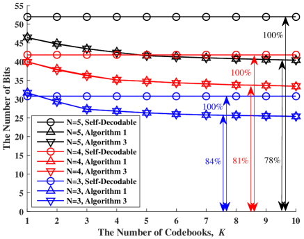
Figure 3: Expected number of bits versus the number of codebooks under discrete user preferences.

Fig. 3 presents the expected number of bits to represent a requested content item versus the number of codebooks under discrete user preferences, where the total number of SPVs with nonzero probability is set to be $J=1000$. These SPVs are uniformly sampled from $\Omega$. It is not surprising that the larger the alphabet, the greater the number of bits needed to represent a requested content item. To demonstrate the potential of edge source coding, we compare our algorithms with a traditional self-decodable method, in which each requested content item is encoded according to its SPV and carries a codebook for decoding. Thus, the self-decodable method encode a content item with SPV $\bm{p}$ into $LH(\bm{p})+\sum_{n=1}^{N}\log p_{n}$ bits. In Fig. 3, it can be seen the proposed DCA based and $k$-means++ based algorithms, i.e., Algorithms 1 and 3, always achieve similar performance. Except the case $N=3$ and $K=1$, Algorithms 1 and 3 use fewer bits to represent a requested content item than the self-decodable method does. When $N=5$ and $K=10$, our algorithms can even save 22% of the total number of bits. For fixed $N$, the number of bits to represent a requested content item decreases with an increase in the number of codebooks. This is because the mismatch between SPVs and codebooks is small when more codebooks are used. However, an increase in the number of codebooks $K$ only slightly reduces the number of bits when $K$ is large.

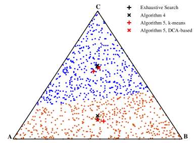
(a) Uniform

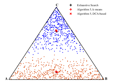
(b) Nonuniform

Figure 4: Edge source coding under uniform and nonuniform user preferences

Fig. 4 illustrates the performance of Algorithms 4 and 5. For the sake of illustration, we set $N=3$ and $K=2$ in the simulation. The notation $A,B,$ and $C$ in these two figures has identical meaning to that in Fig. 2. In the subfigures (a) and (b), the function $f$ is respectively set to be $f=1/{\int_{\bm{p}\in\Omega}d\bm{p}}$ and $f=(||\bm{p}-\bm{p}_{0}||_{2})/{\int_{\bm{p}\in\Omega}||\bm{p}-\bm{p}_{0}||_{2}d\bm{p}}$, where $\bm{p}_{0}=[1/3,1/3,1/3]$ and $||\cdot||_{2}$ denotes the Euclidean norm. Thus, the user preferences are uniform and nonuniform respectively in the two subfigures. The black cross and x mark represent the solutions given by exhaustive search and Algorithm 4, respectively. The red x mark and cross represent the solutions when Algorithm 5 calls Algorithms 1 and 3, respectively. The blue and orange dots represents the sample points when Algorithm 5 runs ($S=1000$ points are sampled). The color of a dot indicates the codebook used by this dot. Fig. 4 reveals that the optimal codebook designs vary with user preferences. It is seen that the codebook designs given by Algorithms 4 and 5 are very close to the optimal solution given by exhaustive search. For the uniform user preferences, the expected numbers of bits resulting from Algorithm 4, Algorithm 5 calling Algorithm 1, Algorithm 5 calling Algorithm 3, and exhaustive search are 29.0682, 29.0486, 29.0816, and 29.0457, respectively. For the considered nonuniform user preferences, the expected numbers of bits resulting from Algorithm 5 calling Algorithm 1, Algorithm 5 calling Algorithm 3, and exhaustive search are 26.2575, 26.2753, and 27.2523. The gaps between the expected numbers of bits given by our algorithms and the optimal are very small.

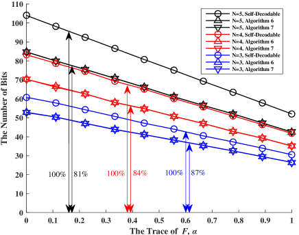
Figure 5: Expected number of bits versus the trace of joint preference matrix for edge source coding with two users.

Fig. 5 presents the number of bits to represent a requested content item versus the similarity of the user preferences for edge source coding with two users. We assume there are $J=1000$ content items which are with SPVs uniformly sampled from $\Omega$. The joint preference matrix $\bm{F}=(f_{i,j})_{J\times J}$ is set to be

$$f_{i,j}=\begin{cases}\frac{\alpha}{J},&\text{if }i=j;\\ \frac{1-\alpha}{J(J-1)},&\text{others.}\end{cases}$$ (47)

Then, the trace of $\bm{F}$ is $\alpha$, which describes the similarity of the two users’ preferences. In Fig. 5, we assume the total numbers of codebooks used by user 1 and user 2 are $K_{1}^{t}=4$ and $K_{2}^{t}=4$. Again, we compare our algorithms with the self-decodable method, in which each content item is attached with a codebook in transmission. It can be seen that the expected number of bits to satisfy user requests almost linearly decrease with the trace of $\bm{F}$. This is due to the fact that higher trace of $\bm{F}$ induces more multicasting opportunities. The DCA based and $k$-means++ based algorithms, i.e., Algorithms 6 and 7, have similar performance. Furthermore, our algorithms always achieve lower number of bits than the self-decodable method does. When $N=5$, our algorithms can save 19% of the total number of bits.

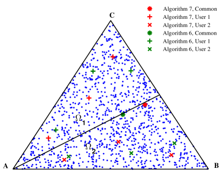
Figure 6: Expected number of bits versus the similarity of user preferences in two-user case.

Fig. 6 illustrates optimal codebook designs for $N=3$ and $K_{1}^{t}=K_{2}^{t}=4$. There are total $J=1000$ content items. We assume user 1 is interested only in content items with SPVs in $\Omega_{1}$ and user 2 is interested only in content items with SPVs in $\Omega_{2}$. The green and red asterisks represents the common codebooks given by Algorithms 6 and 7, respectively. The cross and x mark represents the codebooks exclusively used by user 1 and user 2, respectively. It can be seen both the common codebooks are located around the boundary between $\Omega_{1}$ and $\Omega_{2}$. The codebook designs resulting from the two algorithms differ sharply, which implies the existence of multiple locally optimal solutions. The numbers of bits given by Algorithms 6 and 7 are 51.0691 and 50.9569. Again, the performances of the two algorithms are similar.

VII Conclusion and Directions for Future Work

In this paper, we have studied user preference aware lossless data compression at the edge, where content items are characterized by SPVs and user preferences are described by probability density functions. We have noted that the statistical distributions of symbols over the links generally differ from that in the information source and have presented an edge source coding method, which employs finitely many codebooks to encode the requested content items at the service provider. An optimization problem has been formulated to give the optimal codebook design for edge source coding, which is however nonconvex in general. The optimal solution for edge source coding with one codebook has been given by the method of Lagrange multipliers. Furthermore, an optimality condition has been presented. For edge source coding under discrete user preferences, the optimization problem reduces to a clustering problem. DCA based and $k$-means++ algorithms have been proposed to give codebook designs. For edge source coding under continuous user preferences, an iterative algorithm has been proposed to give a codebook design according to the optimality condition. To provide a codebook design with low computational complexity, a sampling based algorithm has also been proposed. In addition, we have extended edge source coding to the two-user case and codebooks have been designed to utilize the multicasting opportunities. It has been shown that the solutions of the proposed algorithms are close to the optimal. In the two-user case, the expected number of bits needed to represent a requested content item linearly decreases with the trace of the joint preference matrix. Both theoretical analysis and simulations have verified that the optimal codebook design in edge source coding relies on user preferences.

Significant future topics include edge source coding with more than two users, more-refined theoretical analysis on the optimal codebook design and the resulting transmission cost, as well as practical user preference model based on real data.

Here we show the transformation from the optimal solution of problem (14) to that of problem (11). To show that, we only need to show the existence of 0-1 optimal solution of problem (14). The core idea is to improve the solution by removing elements unequal to 0 or 1. Suppose $\{r_{j,k}^{*}:j\in[J],k\in[K]\}$ is an optimal solution of problem (14) and let $R_{\ref{op_2}}(r_{j,k}^{*})$ denote the corresponding optimization value. We have

$$\sum_{k=1}^{K}r_{j,k}^{*}=1,$$ (48)

for $j\in[J]$. From Eq. (18), we can obtain $\{\bm{q}_{k}^{*}:k\in[K]\}$ such that $\bm{q}_{k}^{*}$ and $r_{j,k}^{*}$ form the optimal solution of problem (15). Let $R_{\ref{op_3}}(\bm{q}^{*}_{k},r_{j,k}^{*})$ denote the optimization value of problem (15). Then we have $R_{\ref{op_3}}(\bm{q}^{*}_{k},r_{j,k}^{*})=R_{\ref{op_2}}(r_{j,k}^{*})$. If there exist $j_{0}$ such that $0<r_{j_{0},k}^{*}<1$ for certain values of $k$, we set

$$r_{j,k}^{**}=\begin{cases}r_{j,k}^{*},&\text{if }j\neq j_{0},\\ 1,&\text{if }j=j_{0}\text{ and }k=\arg\min_{k_{0}\in[K]}D(\bm{p}_{j}||\bm{q}_{k_{0}}^{*}),\\ 0,&\text{if }j=j_{0}\text{ and }k\neq\arg\min_{k_{0}\in[K]}D(\bm{p}_{j}||\bm{q}_{k_{0}}^{*}).\end{cases}$$ (49)

Then, $\{r_{j,k}^{**}\}$ is feasible for problem (14). In addition, we have

$$R_{\ref{op_2}}(r_{j,k}^{**})=R_{\ref{op_3}}(\bm{q}^{**}_{k},r_{j,k}^{**})\geq R_{\ref{op_3}}(\bm{q}^{*}_{k},r_{j,k}^{**})\geq R_{\ref{op_3}}(\bm{q}^{*}_{k},r_{j,k}^{*})=R_{\ref{op_2}}(r_{j,k}^{*}),$$ (50)

where $\bm{q}_{k}^{**}$ is derived from Eq. (18) by substituting $\{r_{j,k}^{**}\}$. As a result, $\{r_{j,k}^{**}\}$ is an optimal solution of problem (14). By applying Eq. (49) iteratively, we can remove all the non 0-1 elements of an optimal solution of problem (14) without the loss of optimality.

References

• [1] C. E. Shannon, “A mathematical theory of communication,” Bell System Technical Journal, vol. 27, pp. 379-423, 623-656, July, Oct., 1948
• [2] J. Ziv and A. Lempel, “A universal algorithm for sequential data compression,” IEEE Transactions on Information Theory, vol. 23, no. 3, pp. 337-343, May 1977.
• [3] T. Sikora, “The MPEG-4 video standard verification model,” IEEE Transactions on Circuits and Systems for Video Technology, vol. 7, no. 1, pp. 19-31, Feb. 1997.
• [4] A. Skodras, C. Christopoulos and T. Ebrahimi, “The JPEG 2000 still image compression standard,” IEEE Signal Processing Magazine, vol. 18, no. 5, pp. 36-58, Sept. 2001.
• [5] O. Rottenstreich and J. Tapolcai, “Optimal rule caching and lossy compression for longest prefix matching,” IEEE/ACM Transactions on Networking, vol. 25, no. 2, pp. 864-878, Apr. 2017.
• [6] J. C. S. de Souza, T. M. L. Assis, and B. C. Pal, “Data compression in smart distribution systems via singular value decomposition,” IEEE Transactions on Smart Grid, vol. 8, no. 1, pp. 275-284, Jan. 2017.
• [7] C. J. Deepu, C. Heng, and Y. Lian, “A hybrid data compression scheme for power reduction in wireless sensors for IoT,” IEEE Transactions on Biomedical Circuits and Systems, vol. 11, no. 2, pp. 245-254, Apr. 2017.
• [8] M. Leinonen, M. Codreanu, and M. Juntti, “Distributed distortion-rate optimized compressed sensing in wireless sensor networks,” IEEE Transactions on Communications, vol. 66, no. 4, pp. 1609-1623, Apr. 2018.
• [9] N. Farsad, M. Rao, and A. Goldsmith, “Deep learning for joint source-channel coding of text,” in Proceeding of IEEE International Conference on Acoustics, Speech and Signal Processing (ICASSP), Calgary, Apr. 2018.
• [10] S. Dorner, S. Cammerer, J. Hoydis, and S. t. Brink, “Deep learning based communication over the air,” IEEE Journal of Selected Topics in Signal Processing, vol. 12, no. 1, pp. 132-143, Feb. 2018.
• [11] S. Wang, X. Zhang, Y. Zhang, L. Wang, J. Yang, and W. Wang, “A survey on mobile edge networks: Convergence of computing, caching and communications,” IEEE Access, vol. 5, pp. 6757-6779, Mar. 2017.
• [12] W. Shi, J. Cao, Q. Zhang, Y. Li, and L. Xu, “Edge computing: Vision and challenges,” IEEE Internet of Things Journal, vol. 3, no. 5, pp. 637-646, Oct. 2016.
• [13] T. Taleb, S. Dutta, A. Ksentini, M. Iqbal, and H. Flinck, “Mobile edge computing potential in making cities smarter,” IEEE Communications Magazine, vol. 55, no. 3, pp. 38-43, Mar. 2017.
• [14] K. Zhang, Y. Mao, S. Leng, Y. He, and Y. Zhang, “Mobile-edge computing for vehicular networks: a promising network paradigm with predictive off-loading,” IEEE Vehicular Technology Magazine, vol. 12, no. 2, pp. 36-44, June 2017.
• [15] M. Chen and Y. Hao, “Task offloading for mobile edge computing in software defined ultra-dense network,” IEEE Journal on Selected Areas in Communications, vol. 36, no. 3, pp. 587-597, Mar. 2018.
• [16] Q. Xu, Z. Su, Q. Zheng, M. Luo, and B. Dong, “Secure content delivery with edge nodes to save caching resources for mobile users in green cities,” IEEE Transactions on Industrial Informatics, vol. 14, no. 6, pp. 2550-2559, June 2018.
• [17] S. M. Azimi, O. Simeone, A. Sengupta, and R. Tandon, “Online edge caching and wireless delivery in fog-aided networks with dynamic content popularity,” IEEE Journal on Selected Areas in Communications, vol. 36, no. 6, pp. 1189-1202, June 2018.
• [18] Q. Yuan, H. Zhou, J. Li, Z. Liu, F. Yang, and X. S. Shen, “Toward efficient content delivery for automated driving services: an edge computing solution,” IEEE Network, vol. 32, no. 1, pp. 80-86, Jan. 2018.
• [19] T. X. Vu, S. Chatzinotas, and B. Ottersten, “Edge-caching wireless networks: Performance analysis and optimization,” IEEE Transactions on Wireless Communications, vol. 17, no. 4, pp. 2827-2839, Apr. 2018.
• [20] Z. Chang, L. Lei, Z. Zhou, S. Mao, and T. Ristaniemi, “Learn to cache: Machine learning for network edge caching in the big data era,” IEEE Wireless Communications, vol. 25, no. 3, pp. 28-35, June 2018.
• [21] Y. Lu, W. Chen, and H. V. Poor, “Multicast pushing with content request delay information,” IEEE Transactions on Communications, vol. 66, no. 3, pp. 1078-1092, Mar. 2018.
• [22] Y. Lu, W. Chen, and H. V. Poor, “Coded joint pushing and caching with asynchronous user requests,” IEEE Journal on Selected Areas in Communications, vol. 36, no. 8, pp. 1843-1856, Aug. 2018.
• [23] Q. Yan, W. Chen, and H. V. Poor, “Big data driven wireless communications: A human-in-the-loop pushing technique for 5G systems,” IEEE Wireless Communications, vol. 25, no. 1, pp. 64-69, Feb. 2018.
• [24] Y. Lu, W. Chen, and H. V. Poor, “Source coding at the edge: user preference oriented lossless data compression,” in Proceeding of IEEE International Conference on Communications (ICC), Shanghai, May 2019, to appear.
• [25] K. Shanmugam, N. Golrezaei, A. G. Dimakis, A. F. Molisch and G. Caire, “FemtoCaching: Wireless content delivery through distributed caching helpers,” IEEE Transactions on Information Theory, vol. 59, no. 12, pp. 8402-8413, Dec. 2013.
• [26] T. Zhang, H. Fan, J. Loo, and D. Liu, “User preference aware caching deployment for device-to-device caching networks,” IEEE Systems Journal, vol. 13, no. 1, pp. 226-237, Mar. 2019.
• [27] S. Dernbach, N. Taft, J. Kurose, U. Weinsberg, C. Diot, and A. Ashkan, “Cache content-selection policies for streaming video services,” in Proceeding of IEEE International Conference on Computer Communications (INFOCOM), San Francisco, Apr. 2016.
• [28] Y. Wang, P. Li, L. Jiao, Z. Su, N. Cheng, X. Shen, and P. Zhang, “A data-driven architecture for personalized QoE management in 5g wireless networks,” IEEE Wireless Communications, vol. 24, no. 1, pp. 102-110, Feb. 2017.
• [29] O. Semiari, W. Saad, S. Valentin, M. Bennis, and H. V. Poor, “Context-aware small cell networks: How social metrics improve wireless resource allocation,” IEEE Transactions on Wireless Communications, vol. 14, no. 11, pp. 5927-5940, Nov. 2015.
• [30] X. Wang, Y. Zhang, V. C. M. Leung, N. Guizani, and T. Jiang, ”D2D big data: Content deliveries over wireless device-to-device sharing in large-scale mobile networks,” IEEE Wireless Communications, vol. 25, no. 1, pp. 32-38, Feb. 2018.
• [31] T. M. Cover and J. A. Thomas, Elements of Information Theory, Second Edition, New York: Wiley, 2006.
• [32] D. Arthur and S. Vassilvitskii. “$k$-means++: The advantages of careful seeding.” in Proceedings of the 18th Annual ACM SIAM Symposium on Discrete Algorithms (SODA), New Orleans, Jan. 2007.
• [33] M. H. Protter and C. B. Morrey, College Calculus With Analytic Geometry, Third Edition, Addison-Wesley, 1977.