Deep Convolutional Spiking Neural Networks
for Image Classification

Abstract

Spiking neural networks are biologically plausible counterparts of the artificial neural networks, artificial neural networks are usually trained with stochastic gradient descent and spiking neural networks are trained with spike timing dependant plasticity. Training deep convolutional neural networks is a memory and power intensive job. Spiking networks could potentially help in reducing the power usage. In this work we focus on implementing a spiking CNN using Tensorflow to examine behaviour of the network and empirically study the effect of various parameters on learning capabilities and also study catastrophic forgetting in the spiking CNN and weight initialization problem in R-STDP using MNIST and N-MNIST data sets.

1 Introduction

Deep learning, i.e., the use of deep convolutional neural networks (DCNN ), is a powerful tool for pattern recognition (image classification) and natural language (speech) processing [54][45]. Deep convolutional networks use multiple convolution layers to learn the input data [27] [55] [13]. They have been used to classify the large data set Imagenet [26] with an accuracy of 96.6% [4]. In this work deep spiking networks are considered[48]. This is new paradigm for implementing artificial neural networks using mechanisms that incorporate spike-timing dependent plasticity which is a learning algorithm discovered by neuroscientists [17] [37]. Advances in deep learning has opened up multitude of new avenues that once were limited to science fiction [63]. The promise of spiking networks is that they are less computationally intensive and much more energy efficient as the spiking algorithms can be implemented on a neuromorphic chip such as Intel’s LOIHI chip [7] (operates at low power because it runs asynchronously using spikes [65] [64] [66] [53] [6]). Our work is based on the work of Masquelier and Thorpe [39] [38], and Kheradpisheh et al. [24] [23]. In particular a study is done of how such networks classify MNIST image data [29] and N-MNIST spiking data [46]. The networks used in [24] [23] consist of multiple convolution/pooling layers of spiking neurons trained using spike timing dependent plasticity (STDP [56]) and a final classification layer done using a support vector machine (SVM) [18].

1.1 Spike Timing Dependant Plasticity (STDP)

Spike timing dependant plasticity (STDP) [36] has been shown to be able to detect hidden (in noise) patterns in spiking data [38]. Figure 1 shows a simple 2 layer fully connected network with $N$ input (pre-synaptic) neurons and 1 output neuron. The spike signals $s_{i}(t)$ are modelled as being either 0 or 1 in one millisecond increments. That is, 1 msec pulse of unit amplitude represents a spike while a value of 0 represents no spike present. See the left side of the Figure 1. Each spike signal has a weight (synapse) associated with it which multiplies the signal to obtain $w_{i}s_{i}(t)$ which is called the post synaptic potential due to the $i^{th}$ input neuron. These potentials are then summed as

$$V(t)=\sum_{i=1}^{N}w_{k}s_{k}(t).$$

$V(t)$ is called the membrane potential of the output neuron. At any time $t$ if the membrane potential $V(t)$ is greater than a specified threshold $\gamma$, i.e., if

$$V(t)>\gamma$$

then the output neuron spikes. By this we mean that the output neuron produces a 1 msec pulse of unit amplitude. See the right side of Figure 1.

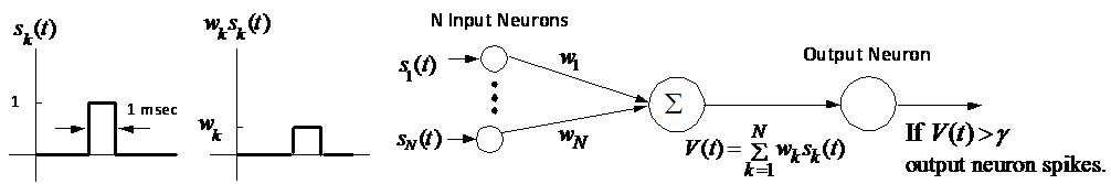
Figure 1: The neurons $s_{i},i=1,...,N$ are the pre-synaptic neurons and the output neuron is the post-synaptic neuron.

Denote the input spike pattern $s(t)$ as

$$s(t)=\left[\begin{array}[c]{c}s_{1}(t)\\ s_{2}(t)\\ \vdots\\ s_{N}(t)\end{array}\right]$$

Let $t_{1}<t_{2}<t_{3}<\cdots$ be a sequence of times for which the spike pattern is fixed, that is, $s_{fixed}=s(t_{1})=s(t_{2})=s(t_{3})=\cdots$ while at all other times the values $s_{i}(t)$ are random (E.g., $P(s_{i}(t)=1)=0.01$ and $P(s_{i}(t)=0)=0.99$). The idea here is that the weights can be updated according to an unsupervised learning rule that results in the output spiking if and only if the fixed pattern is present. The learning rule used here is called spike timing dependent plasticity or STDP. Specifically, we used a simplified STDP model as in given as [24]

$$w_{i}\leftarrow w_{i}+\Delta w_{i},\text{ \ }\Delta w_{i}=\begin{cases}-a^{-}w_{i}(1-w_{i}),\ \ \text{if}\ \ t_{out}-t_{i}<0\\ +a^{+}w_{i}(1-w_{i}),\ \ \text{if}\ \ t_{out}-t_{i}\geq 0.\end{cases}$$

Here $t_{i}$ and $t_{out}$ are the spike times of the pre-synaptic (input) and the post-synaptic (output) neuron, respectively. That is, if the $i^{th}$ input neuron spikes before the output neuron spikes then the weight $w_{i}$ is increased otherwise the weight is decreased. Learning refers to the change $\Delta w_{i}$ in the (synaptic) weights with $a^{+}$ and $a^{-}$ denoting the learning rate constants. These rate constants are initialized with low values $(0.004,0.003)$ and are typically increased as learning progresses. This STDP rule is considered simplified because the amount of weight change doesn’t depend on the time duration between pre-synaptic and post-synaptic spikes.

To summarize, if the pre-synaptic (input) neuron spikes before post-synaptic (output) neuron, then the synapse is increased. If the pre-synaptic neuron doesn’t spike before the post-synaptic neuron then it is assumed that the pre-synaptic neuron will spike later and the synapse is decreased.

The membrane potential profile of the type of output neuron considered here looks as shown in the Figure 2. In Figure 2 the output neuron is shown to receive a spike at 1 msec, two spikes at 2 msec and another two spikes at 3 msec. The output neuron spikes at time 3 msec as its membrane potential exceeded the threshold ($\gamma=4.5$).

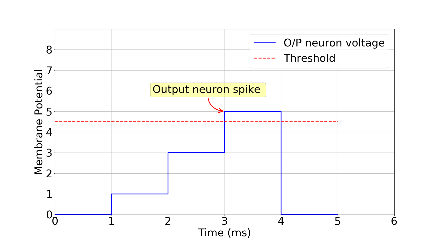
Figure 2: Spike generation by an output neuron.

Figure 3 shows a raster plot of an input neuron versus its spike times for the first 54 msecs. Figure 3 shows $N=100$ input neurons and at time $t$ a dot $\ast$ denotes a spike while an empty space denotes no spike. Red dots in the plot indicates a spike as part of a fixed pattern of spikes. In Figure 3 the pattern presented to the output neuron is 5 msec long in duration. The blue part of Figure 3 denotes random spikes being produced by the input neurons (noise). On close observation of Figure 3 one can see that fixed spike pattern in red is presented at time 0, time 13, and time 38.

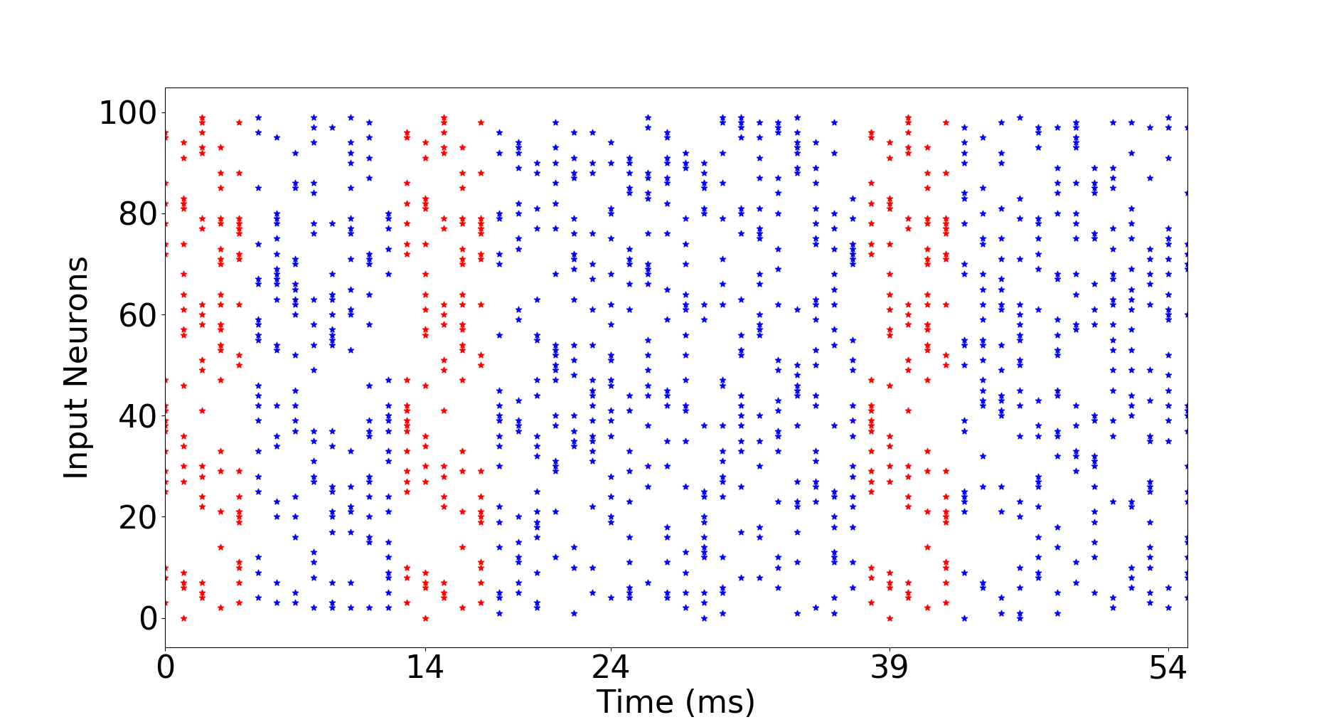
Figure 3: The pattern is red and has a duration of 5 miliseconds. This pattern is presented recurrently to the network at random times. The random noisy spikes are represented in blue.

Using only the above STDP learning rule, the output neuron learns to spike only when the fixed pattern $s_{fixed}$ is produced by the input neurons. With the weights $w_{i}$ set randomly from normal distribution, i.e., $w_{i}\sim\mathcal{N}(0.5,0.05)$ Figure 4 (top plot) shows the output spiking randomly for the first 50 msecs. However after about 2000 msec, Figure 4 (middle plot) shows the output neuron starts to spike selectively, though it incorrectly spikes at times when the pattern is not present. Finally, after about 3000 msec, Figure 4 (bottom plot) shows that the output neuron spikes only when the pattern is present.

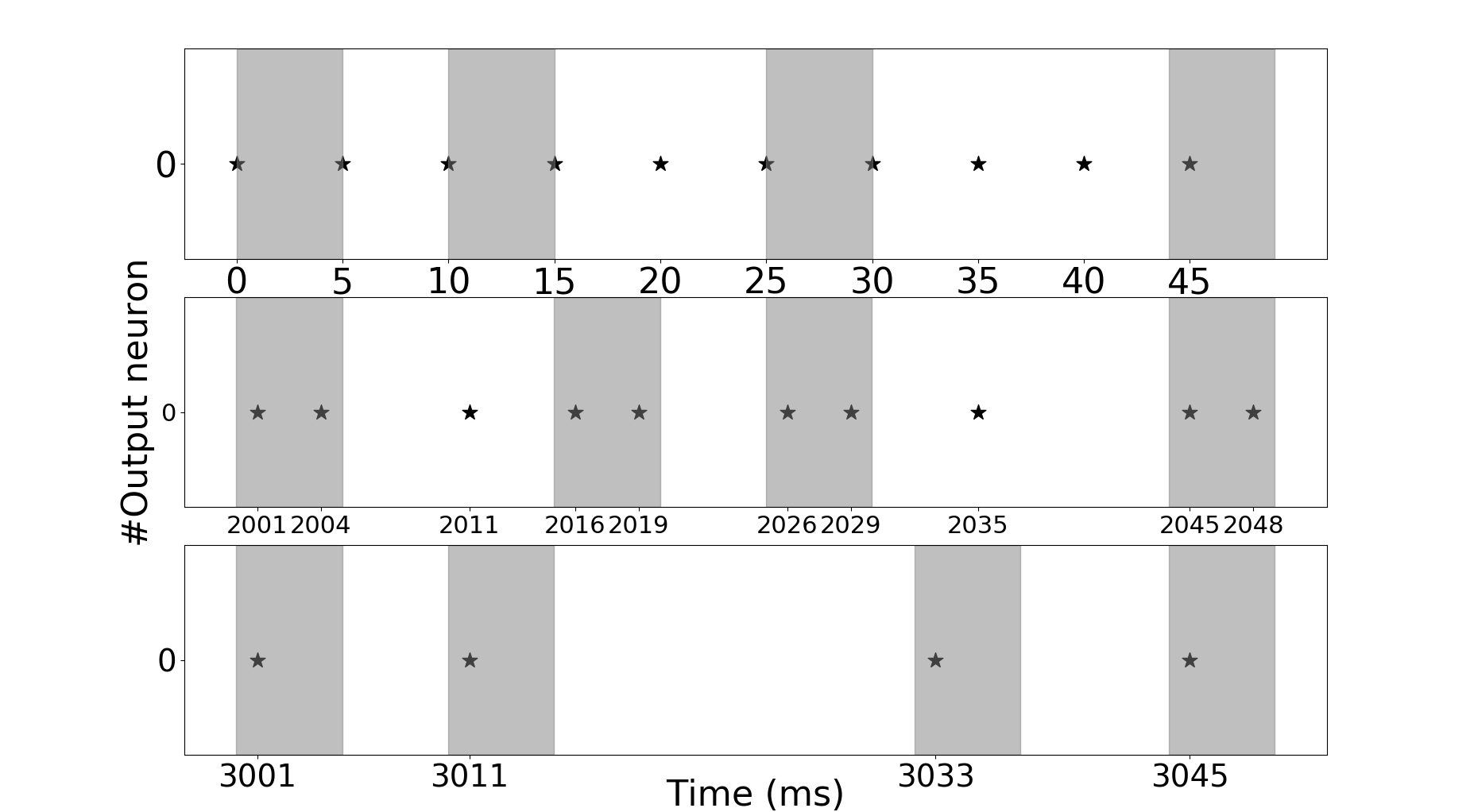
Figure 4: The grey box indicates the fixed pattern being produced by the input neurons $s_{i}.$

1.2 Convolution operation

In this work spiking convolutional neural networks (SCNN) are used for feature extraction. A short explanation of convolution is now presented. Figure 5 shows a convolution operation on an input image.

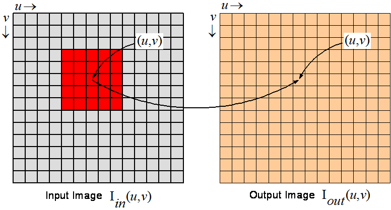
Figure 5: Convolution operation.

Let

$$W_{C}(i,j),\text{ \ \ }0\leq i,j\leq 4$$

denote a $5\times 5$ convolution weight kernel (filter) indicated by the red square Figure 5 above. With the kernel centered on the location $(u,v)$ of the input image $\mathbf{I}_{in}(u,v)$ ($0\leq u,v\leq 14$) the value $\mathbf{I}_{out}(u,v)$ ($0\leq u,v\leq 14$) of the output image at $(u,v)$ is given by

$$\mathbf{I}_{out}(u,v)=\sum_{j=-2}^{j=2}\sum_{i=-2}^{i=2}\mathbf{I}_{in}(u+i,v+j)W_{C}(i,j).$$

Note that the shape of the output image is same as the input image, such convolutions are called same mode convolutions.

Convolution networks are used to detect features in images. To explain, consider the convolution kernel $W_{C1}(i,j,1)$ as shown in Figure 6. This kernel is used to find vertical lines of spikes at any location of the spiking input image. For example, at the location $(u,v)$ at time $\tau$ the kernel is convolved with the spiking image to give

$$\sum_{j=-2}^{2}\sum_{i=-2}^{2}s_{in}(u+i,v+j,\tau)W_{C1}(i,j,1).$$

If there is a vertical line of spikes in the spiking image that matches up with the kernel, then this result will be a maximum (maximum correlation of the kernel with the image). The accumulated membrane potential for the neuron at $(u,v)$ of map1 of the Conv1 layer is given by

$$V_{m}(u,v,t,1)=\sum\limits_{\tau=0}^{t}\left(\sum_{j=-2}^{2}\sum_{i=-2}^{2}s_{in}(u+i,v+j,\tau)W_{C1}(i,j,1)\right).$$

The neuron at $(u,v)$ of map 1 of the Conv1 layer then spikes at time $t$ if

$$V_{m}^{(1)}(u,v,t)\geq\gamma_{C1}$$

where $\gamma_{C1}$ is the threshold. If the neuron at $(u,v)$ in map 1 of Conv1 spikes then a vertical line of spikes have been detected in the spiking image centered at $(u,v)$.

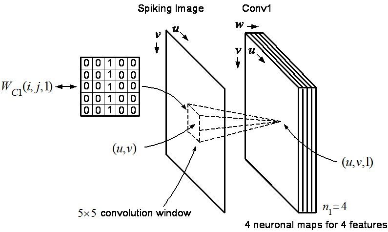
Figure 6: Feature detection.

Figure 7 shows that map 2 (second feature map) of Conv1 is used to detect a line of spikes at 45 degrees. The third feature map (map 3) is used to detect a line of spikes at 135 degrees and the fourth feature map (map 4) is used to detect a horizontal line of spikes.

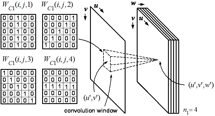
Figure 7: Feature detection.

A typical SCNN has multiple layers. Each layer will have multiple feature maps (simply, maps).

2 Literature survey

In $1951$ Hubel and Wiesel [19] showed that a cat’s neurons in primary visual cortex are tuned to simple features and the inner regions of the cortex combined these simple features to represent complex features. The neocognitron model was proposed in $1980$ by Fukushima to explain this behavior [12]. This model didn’t require a ”teacher” (unsupervised) to learn the inherent features in the input, akin to the brain. The neocognitron model is a forerunner to the spiking convolutional neural networks considered in this work. These convolutional layers are arranged in layers to extract features in the input data. The terminology ”deep” CNNs refers to a network with many such layers. However, the deep CNNs used in industry (Google, Facebook, etc.) are fundamentally different in that they are trained using supervision (back propagation of a cost function). Here our interest is to return to the neocognitron model using spiking convolutional layers in which all but the output layer is trained without supervision.

2.1 Unsupervised networks

A network equipped with STDP [36] and lateral inhibition was shown to develop orientation selectivity similar to the visual frontal cortex in a cat’s brain [8] [68]. STDP was shown to facilitate approximate Bayesian computation in the visual cortex using expectation-maximization [44]. STDP is used for feature extraction in multi-layer spiking CNNs. It has been shown that deeper layers combine the features learned in the earlier layers in order to represent advanced features, but at the same time sparsity of the network spiking activity is maintained [47] [24] [23] [10] [39] [62] [61] [67] [59]. In [9] a fully connected networks trained using unsupervised STDP and homeostasis achieved a 95.6% classification accuracy on the MNIST data set.

2.2 Reward modulated STDP

Mozafari et al. [41] [42] proposed reward modulated STDP (R-STDP) to avoid using a support vector machine (SVM) as a classifier. It has been shown that the STDP learning rule can find spiking patterns embedded in noise [38]. That is, after unsupervised training, the output neuron spikes if the spiking pattern is input to it. A problem with this unsupervised STDP approach is that as this training proceeds the output neuron will spike when just the first few milliseconds of the pattern have been presented. (For example, the pattern in Figure 3 is 5 msecs long and the output starts to spike when only (say) the first 2 msecs of the pattern have been presented to it though it should only spike after the full 5 msec pattern has been presented. Mozafari et al showed in [42] that R-STDP helps to alleviate this problem.

When unsupervised training methods are used, the features learned in the last layer are used as input to an SVM classifier [23][24] or a simple two or three layer back propagation classifier [58]. In contrast, R-STDP uses a reward or punishment signal (depending upon if the prediction is correct or not) to update the weights in the final layer of a multi-layer (deep) network. Spiking convolutional networks are successful in extracting features [42][23][24]. Because R-STDP is a supervised learning rule, the extracted features (reconstructed weights) more closely resemble the object they detect and thus can (e.g.,) more easily differentiate between a digit “1” and a digit ”7” compared to STDP. That is, reward modulated STDP seems to compensate for the inability of the STDP to differentiate between features that closely resemble each other [11] [32] [41] [57]. It is also reported in [41] that R-STDP is more computationally efficient. However, R-STDP is prone to over fitting, which is alleviated to some degree by scaling the rewards and punishments (e.g., receiving higher punishment for a false positive and a lower reward for a true positive) [41] [42]. In more detail, the reward modulated STDP learning rule is:

If a reward signal is generated then the weights are updated according to

$$\begin{cases}\Delta w_{ij}=+\frac{N_{miss}}{N}a_{r}^{+}w_{ij}(1-w_{ij})&\text{ if}\ t_{j}-t_{i}\leq 0\\ \Delta w_{ij}=-\frac{N_{miss}}{N}a_{r}^{-}w_{ij}(1-w_{ij})&\text{ if}\ t_{j}-t_{i}>0.\end{cases}$$

If a punishment signal is generated then the weights are updated according to

$$\begin{cases}\Delta w_{ij}=-\frac{N_{hit}}{N}a_{p}^{+}w_{ij}(1-w_{ij})&\text{ if}\ t_{j}-t_{i}\leq 0\\ \Delta w_{ij}=+\frac{N_{hit}}{N}a_{p}^{-}w_{ij}(1-w_{ij})&\text{ if}\ t_{j}-t_{i}>0.\end{cases}$$

Here $t_{j}$ and $t_{i}$ are the pre- and post-synaptic times, respectively. For every $N$ input images, $N_{miss}$ and $N_{hit}$ are number of misclassified and correctly classified samples. Note that $N_{miss}+N_{hit}=N$, if the decision of the network is based on the maximum potential of the network, if the decision of the network is based on the early spike $N_{miss}+N_{hit}\leq N$ because there might be no spikes for some inputs.

2.3 Spiking networks with back propagation

[30] used two unsupervised spiking CNNs for feature extraction. Then initializing with these weights, they used a type of softmax cost function for classification with the error back propagated through all layers. They were able to obtain a classification accuracy 99.1% on the MNIST data set. A similar approach with comparable accuracy was carried by [60]. Other methods such as computing the weights on conventional (non spiking) CNNs trained using the back propagation algorithm and then converting them to work on spiking networks have been shown to achieve an accuracy of 99.4% on MNIST data set and 91.35% on CIFAR10 data set [52]. An approximate back propagation algorithm for spiking neural networks was proposed in [2] [31]. In [21] a spiking CNN with 15C5-P2-40C5-P2-300-10 layers using error back propagation through all the layers reported an accuracy of 99.49% on the MNIST data set. The authors in [21] also classified the N-MNIST data set using a fully connected three-layer network with 800 neurons in the hidden layer and reported an accuracy of 98.84%.

Another approach to back propagation in spiking networks is the random back propagation approach. First the standard back propagation equations in (non-spiking) neural networks is now summarized [45]. The gradient of a quadratic cost $C=\sum_{i=1}^{n_{0ut}}(y-a^{L})^{2}$ gives the error from the last layer as

$$\delta^{L}=\frac{\partial C}{\partial a^{L}}\sigma^{\prime}(z^{L}).$$ (1)

$a^{L}$ is the activation of the neurons in the output layer, $\sigma$ is the activation function and $z$ is the net input to the output layer. This error on the last layer is back propagated according to

$$\delta^{l}=((W^{l+1})^{T}\delta^{l+1})\odot\sigma^{\prime}(z^{l})$$ (2)

where $W^{l+1}$ are the weights connecting the $l^{th}$ and ($l+1)^{th}$ layer. The weights and biases are updated as follows:

$$\frac{\partial C}{\partial b_{j}^{l}}=\delta_{j}^{l}$$ (3)

$$\frac{\partial C}{\partial W_{jk}^{l}}=a_{k}^{l-1}\delta_{j}^{l}$$ (4)

In equation (2), the weight matrix $W^{l+1}$ connecting the $l^{th}$ and ($l+1)^{th}$ layer is the same as the weight matrix used in forward propagation to calculate the activations $a^{l+1}$ of $(l+1)^{th}$ layer. This is bothersome to the neuroscience community as this is not biologically plausible [33] [15] [51]. This is referred to as the weight transport problem. Lillicrap et al. [34] showed that the back propagation algorithm works well even if $W^{l+1}$ in equation (2) is replaced with another fixed random matrix $(W^{\prime})^{l+1}$. This eliminates the requirement of weight symmetry, i.e., the same weights for forward and backward propagations. A neuromorphic hardware specific adaptation of random error back propagation that solves the weight transport problem was introduced by [43] and was shown to achieve an error rate of 1.96% for the MNIST data set. The cost function in [43] is defined as

$$L_{sp}=0.5{\displaystyle\sum\limits_{i}}(v_{i}^{p}(t)-v_{i}^{l}(t))^{2}$$ (5)

where $e_{i}(t)$ is the error of the $i^{th}$ output neuron and $v^{p}$ and $v^{l\text{ }}$are the firing rates of the prediction neuron and the label neuron.

$$\dfrac{\partial L_{sp}}{\partial W_{ij}}=-{\displaystyle\sum\limits_{i}}e_{i}(t)\dfrac{\partial v_{i}^{p}(t)}{\partial W_{ij}}$$ (6)

In equation (6), $\dfrac{\partial v_{i}^{p}(t)}{\partial W_{ij}}$ was approximated as

$$\dfrac{\partial v_{i}^{p}(t)}{\partial W_{ij}}\propto\begin{cases}1&\text{ if}\ s_{j}^{h}(t)=1\text{ and }b_{\min}<I_{i}(t)<b_{\max}\\ 0&\text{ otherwise}\end{cases}$$ (7)

Where $I_{i}(t)$ is the current entering into $i^{th}$ post-synaptic neuron and $s_{j}^{h}(t)=1$ indicates the presence of a pre-synaptic spike. For more details see [43]. The weight update for the last layer is then

$$\Delta W_{ij}^{E}\propto\begin{cases}-e_{i}(t)&\text{ if}\ s_{j}^{h}(t)=1\text{ and }b_{\min}<\text{\ }I_{i}(t)<b_{\max}\\ 0&\text{ otherwise}\end{cases}$$ (8)

The weight update for hidden layers is

$$\Delta w_{ij}^{C}\propto\begin{cases}-\sum_{k}g_{ik}e_{k}^{E}(t)&\text{ if}\ s_{j}^{C}(t)=1\text{ and }b_{\min}<\text{\ }I_{i}(t)<b_{\max}\\ 0&\text{ otherwise}\end{cases}$$ (9)

where $e_{k}^{E}(t)$ denotes the error term of the $k^{th}$ neuron in the output layer and $g_{ik}$ is a fixed random number as suggested by the random back propagation algorithm. In the work to be reported below, random back propagation is not used. Specifically, when back propagation is used below, it is only between the penultimate and output layer making random back propagation unnecessary.

2.4 Spike encoding

Spikes are either rate coded or latency coded [14] [25] [50] [3]. Rate coding refers to the information encoded by the number of spikes per second (more spikes per time carries more information) In this case the spike rate is determined by the mean rate of a Poisson process. Latency encoding refers to the information encoded in the time of arrival of a spike (earlier spikes carry more information). The raster plot of Figure 3 shows that spatiotemporal information is provided by the input spikes to the output neuron. That is, which input neuron is spiking (spatio) and the time a neuron spikes (temporal) is received by the output neuron. The spiking networks use this spatiotemporal information to extract features (e.g., detect the pattern in Figure 3) in the input data [16] [40].

2.5 Realtime spikes

Image sensors (silicon retinas) such as ATIS [49] and eDVS [5] provide (latency encoded) spikes as their output. These sensors detect changes in pixel intensities. If the pixel value at location $(u,v)$ increases then an ON-center spike is produced while if the pixel value decreased an OFF-center spike is produced. Finally, if the pixel value does not change, no spike is produced. The spike data from an image sensor is packed using an address event representation (AER [20]) protocol and can be accessed using serial communication ports. A recorded version of spikes from eDVS data set was introduced in [35] and a similar data set of MNIST images recorded with ATIS data set was introduced in [46].

3 Background

3.1 Spiking Images

We have considered the standard $27\times 27$ grey-scale MNIST images [29] and the spiking N-MNIST data files [46] for our experiments. In the case of the MNIST images we needed to convert them to spikes. This was done by first using both an on-center and an off-center Difference of Gaussian (DoG) convolution filter $\Gamma_{\sigma_{1},\sigma_{2}}(i,j)$ for edge detection given by

$$K_{\sigma_{1},\sigma_{2}}(i,j)=\left\{\begin{array}[c]{cl}\dfrac{1}{2\pi\sigma_{1}^{2}}e^{-\dfrac{i^{2}+j^{2}}{2\sigma_{1}^{2}}}-\dfrac{1}{2\pi\sigma_{2}^{2}}e^{-\dfrac{i^{2}+j^{2}}{2\sigma_{2}^{2}}}&\text{for }-3\leq i\leq 3,-3\leq j\leq 3\\ 0&\text{otherwise}\end{array}\right.$$

where $\sigma_{1}=1,\sigma_{2}=2$ for the on-center and $\sigma_{1}=2,\sigma_{2}=1$ for the off-center.

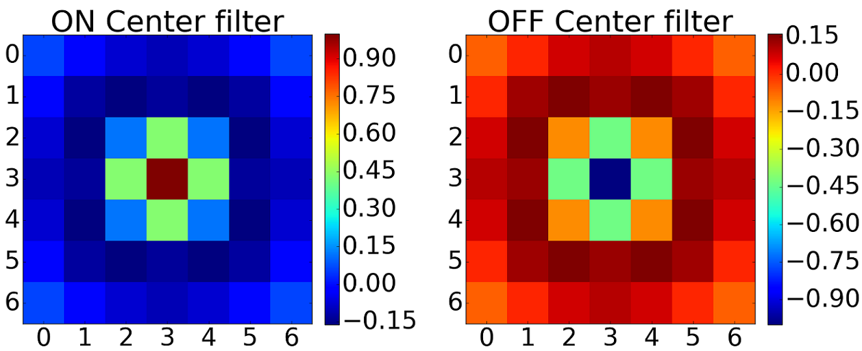
Figure 8: On center filter has higher values in the center whereas the off center filter has lower values in the center. Colour code indicates the filter values.

With the input image $\mathbf{I}_{in}(u,v)\in\mathbb{R}^{27\times 27}$, the output of each of the two DoG filters is computed using the same mode convolution

$$\Gamma_{\sigma_{1},\sigma_{2}}(u,v)=\sum_{j=-3}^{j=3}\sum_{i=-3}^{i=3}\mathbf{I}_{in}(u+i,v+j)K_{\sigma_{1},\sigma_{2}}(i,j)\text{ \ for }0\leq u\leq 26,0\leq v\leq 26.$$

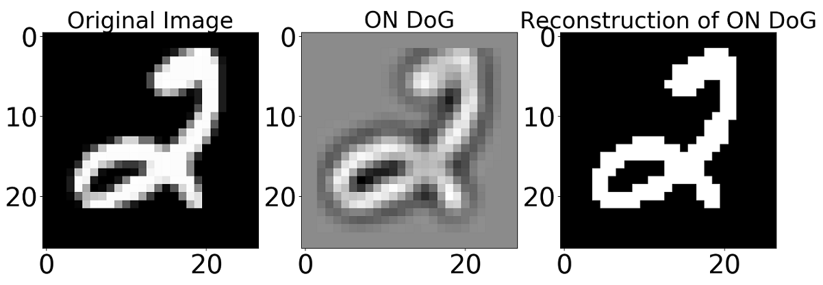
Figure 9: Left: Original grey-scale image. Center: Output of the ON DoG filter. Right: Accumulation of spikes (white indicates a spike black indicates no spike).

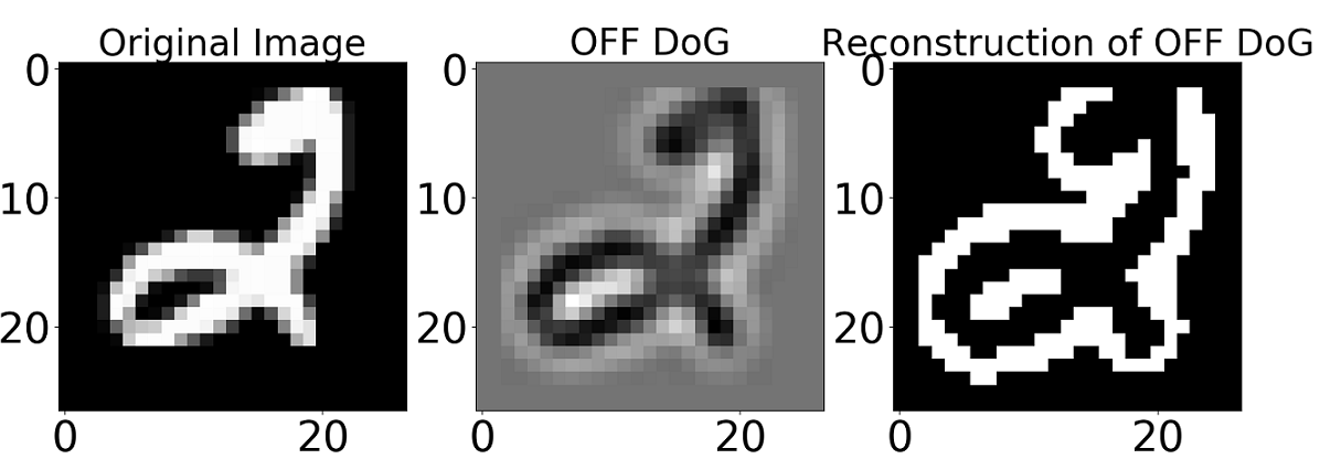
Figure 10: Left: Original grey-scale image. Center: Output of the OFF DoG filter. Right: Accumulation of spikes (white indicates a spike black indicates no spike).

Then these two resulting “images” were then converted to an on and an off spiking image by  At each location $(u,v)$ of the output image $\Gamma_{\sigma_{1},\sigma_{2}}(u,v)$ a unit spike $s_{(u,v)}$ is produced if and only if ([22])

$$\Gamma_{\sigma_{1},\sigma_{2}}(u,v)>\gamma_{DoG}=50.$$

The spike signal $s_{(u,v)}(t)$ is temporally coded (rank order coding[8]) by having it delayed “leaving” the Difference of Gaussian image $\Gamma_{\sigma_{1},\sigma_{2}}(u,v)$ by the amount

$$\tau_{(u,v)}=\frac{1}{\Gamma_{\sigma_{1},\sigma_{2}}(u,v)}\text{ in milliseconds}.$$

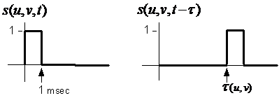
Figure 11: Spike signal

That is, the more $\Gamma_{\sigma_{1},\sigma_{2}}(u,v)$ exceeds the threshold $\gamma_{DoG}$ the sooner it leaves $\Gamma_{\sigma_{1},\sigma_{2}}(u,v)$ or equivalently, the value of $\Gamma_{\sigma_{1},\sigma_{2}}(u,v)$ is encoded in the value $\tau_{(u,v)}.$

For all experiments the arrival times of the spikes were sorted in ascending order and then (approximately) equally divided into 10 bins (10 times in Figure 12). The raster plot shows which neurons (pixels of $\Gamma_{\sigma_{1},\sigma_{2}}(u,v)$) spiked to make up bin 1 (time 0), bin 2 (time 1), etc. Figure 12 shows an example for ON center cell spikes. In all the experiments each image is encoded into 10 msec (10 bins) and there is a 2 msec silent period between every image.

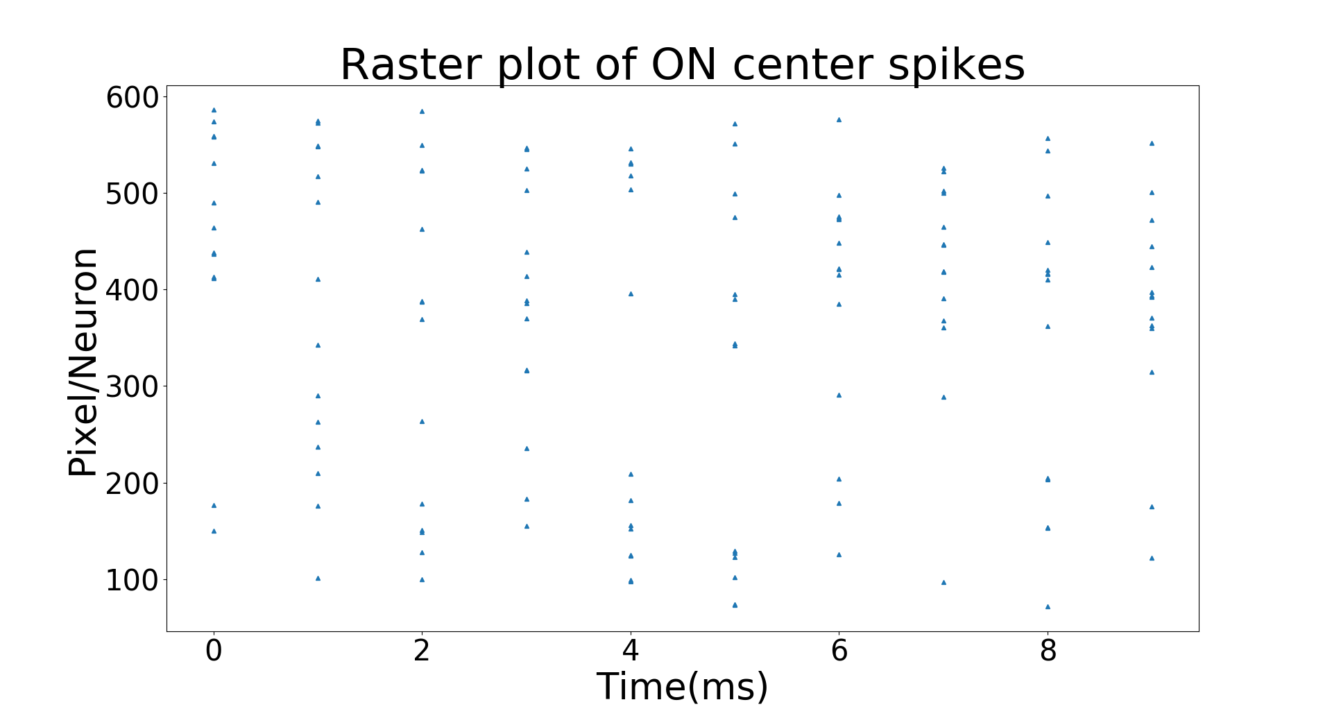
Figure 12: Rasterplot of spikes for an on centre cell. Blue dots in the plot indicates the presence of a spike for a particular neuron and bin (timestep).

3.2 Network Description

We have a similar network as in [24][23] as illustrated in Figure 13. We let $s_{L1}(t,k,u,v)$ denote the spike signal at time $t$ emanating from the $(u,v)$ neuron of spiking image $k$ where $k=0$ (ON center) or $k=1$ (OFF center). The L2 layers consists of 30 maps with each map having its own convolution kernel (weights) of the form

$$W_{C1}(w,k,i,j)\in\mathbb{R}^{2\times 5\times 5}\text{ \ for \ }w=0,1,2,...,29$$

The “membrane potential” of the $(u,v)$ neuron of map $w$ ($w=0,1,2,...,29$) of L2 at time $t$ is given by the valid mode convolution

$$V_{L2}(t,w,u,v)=\sum_{\tau=0}^{t}\left(\sum_{k=0}^{1}\sum_{i=0}^{4}\sum_{i=0}^{4}s_{L1}(\tau,k,u+i,v+j)W_{C1}(w,k,i,j)\right)\text{\ \ for }(0,0)\leq(u,v)\leq(22,22)$$

If at time $t$ the potential

$$V_{L2}(t,w,u,v)>\gamma=15$$

then the neuron at $(w,u,v)$ emits a unit spike.

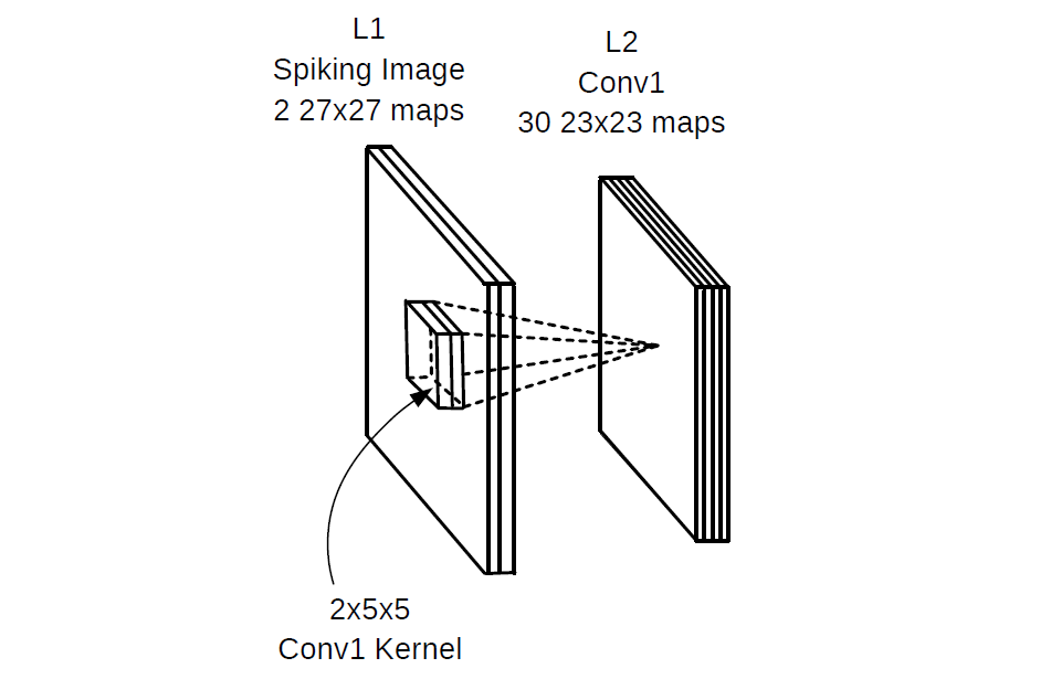
Figure 13: Demonstration of convolution with a 3D kernel.

3.2.1 Convolution Layers and STDP

At any time $t,$ all of the potentials $V_{L2}(t,w,u,v)$ for $(0,0)\leq(u,v)\leq(22,22)$ and $w=0,1,2,...,29$ are computed (in theory this can all be done in parallel) with the result that neurons in different locations within a map and in different maps may have spiked. In particular, at the location $(u,v)$ there can be multiple spikes (up to 30) produced by different maps. The desire is to have different maps learn different features of an image. To enforce this learning, lateral inhibition and STDP competition are used [24].

Lateral Inhibition

To explain lateral inhibition, suppose at the location $(u,v)$ there were potentials $V_{L2}(t,w,u,v)$ in different maps $w$ at time $t$ that exceeded the threshold $\gamma$ Then the neuron in the map with the highest potential $V_{L2}(t,w,u,v)$ at $(u,v)$ inhibits the neurons in all the other maps at the location $(u,v)$ from spiking till the end of the present image (even if their potential exceeded the threshold). Figure 14 shows the accumulated spikes (from an MNIST image of “5”) from all 30 maps at each location $(u,v)$ with lateral inhibition not being imposed. For example, at location (19,14) in Figure 14 the color code is yellow indicating in excess of 20 spikes, i.e., more than 20 of the maps produced a spike at that location.

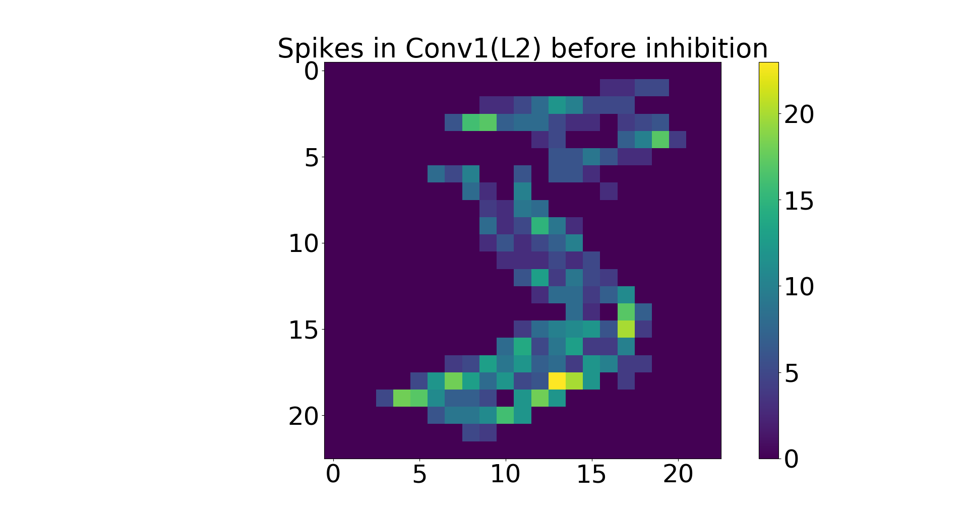
Figure 14: Accumulation of spikes in L2 without lateral inhibition.

Figure 15 shows the accumulation of spikes from all 30 maps, but now with lateral inhibition imposed. Note that at each location there is either 1 spike or no spike as indicated by the color code.

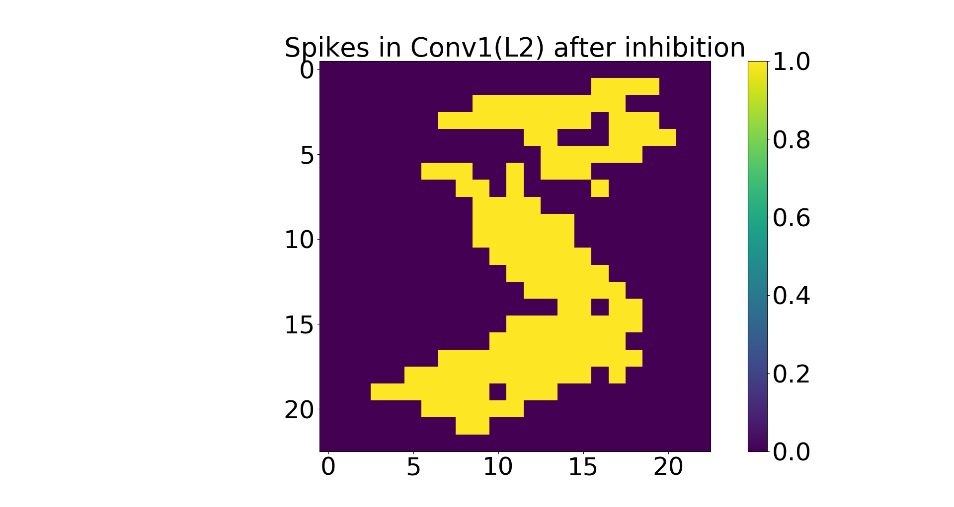
Figure 15: Accumulation of spikes from the MNIST digit “5” with lateral inhibition imposed.

STDP Competition

After lateral inhibition, we consider each map that had one or more neurons whose potential $V$ exceeded $\gamma.$ Let these maps be $w_{k1},w_{k2},...,w_{km}$ where $0\leq k_{1}<k_{2}<\cdots<k_{m}\leq 29$. Then in each map $w_{ki}$ we locate the neuron in that map that has the maximum potential value. Let $(u_{k1},v_{k1}),(u_{k2},v_{k2}),...,(u_{km},v_{km})$ be the location of these maximum potential neurons in each map. Then neuron $(u_{ki},v_{ki})$ inhibits all other neurons in map $w_{ki}$ from spiking for the remainder of the time steps of that spiking image. Further, these $m$ neurons can inhibit each other depending on their relative location as we now explain. Suppose neuron $(u_{ki},v_{ki})$ of map $w_{ki}$ has the highest potential of these $m$ neurons. Then, in an $11\times 11$ area centered about $(u_{ki},v_{ki}),$ this neuron inhibits all neurons of all the other maps in the same $11\times 11$ area. Next, suppose neuron $(u_{kj},v_{kj})$ of map $w_{kj}$ has the second highest potential of the remaining $m-1$ neurons. If the location $(u_{kj},v_{kj})$ of this neuron was within the $11\times 11$ area centered on neuron $(u_{ki},v_{ki})$ of map $w_{ki},$ then it is inhibited. Otherwise, this neuron at $(u_{kj},v_{kj})$ inhibits all neurons of all the other maps in a $11\times 11$ area centered on it. This process is continued for the remaining $m-2$ neurons. In summary, there can be no more than one neuron that spikes in the same $11\times 11$ area of all the maps.

Figure 16 shows the spike accumulation after both lateral inhibition and STDP competition have been imposed. The figure shows that there is at most one spike from all the maps in any $11\times 11$ area.

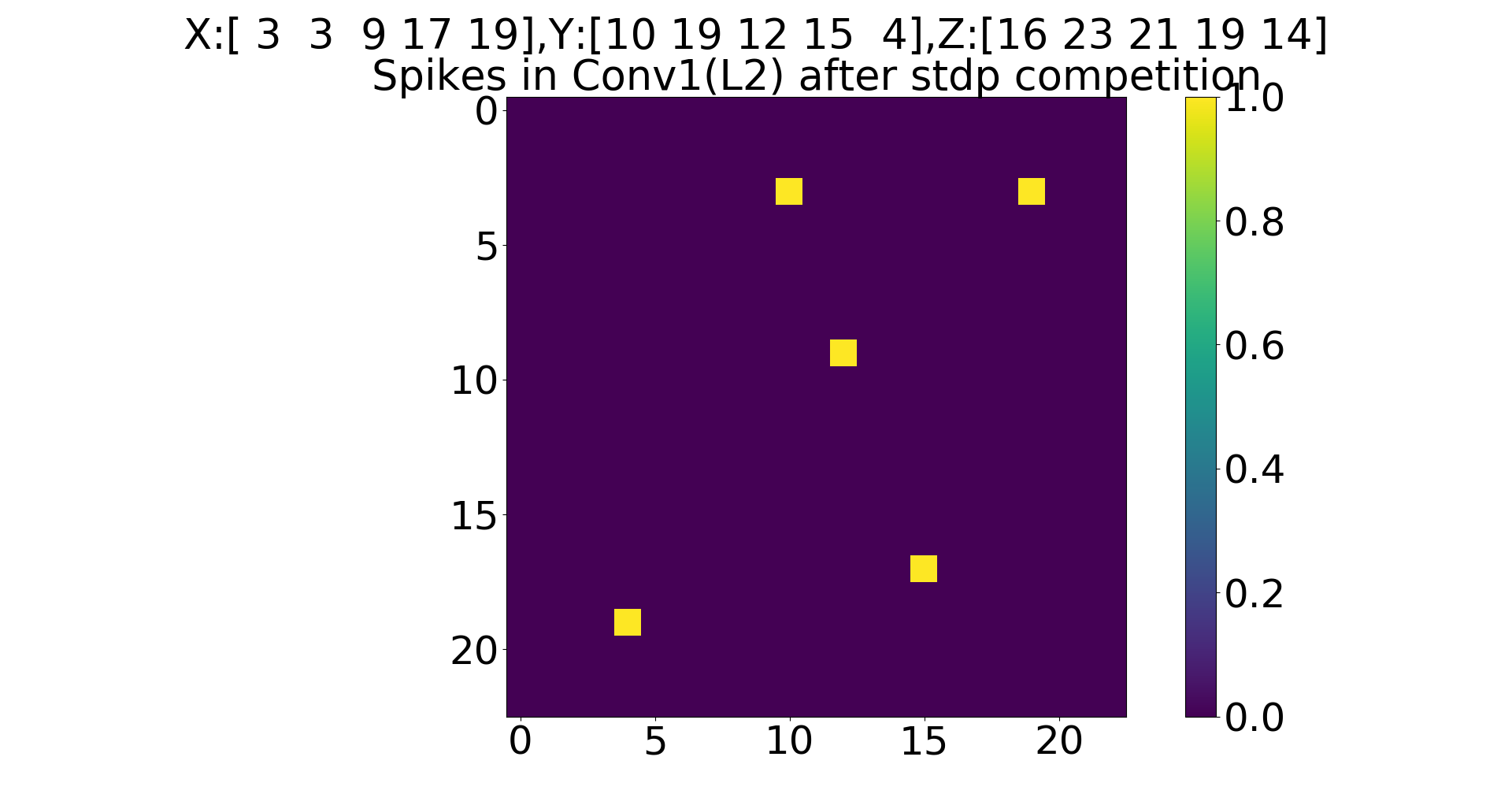
Figure 16: Accumulation of spikes with both lateral inhibition and STDP competition imposed.

Lateral Inhibition and STDP inhibition enforce sparse spike activity and, as a consequence, the network tends to spike sparsely

Spike Timing Dependent Plasticity (STDP)

Only those maps that produced a spike (with lateral inhibition and STDP competition imposed) have their weights (convolution kernels) updated using spike timing dependent plasticity. Let $w_{ij}$ be the weight connecting the $j^{th}$ pre-synaptic neuron in the L1 layer to $i^{th}$ post-synaptic neuron in the L2 layer. If the $i^{th}$ post-synaptic neuron spikes at time $t_{i}$ with the pre-synaptic neuron spiking at time $t_{j}$ then the weight $w_{ij}$ is updated according to the simplified STDP rule [8]

$$w_{ij}\longleftarrow w_{ij}+\Delta w_{ij},\text{ \ where \ }\Delta w_{ij}=\begin{cases}+a^{+}w_{ij}(1-w_{ij})\ \ \text{if }\ t_{i}>t_{j}\\ -a^{-}w_{ij}(1-w_{ij})\ \ \text{otherwise.}\end{cases}$$

The parameters $a^{+}>0$ and $a^{-}>0$ are referred to as learning rate constants. $a^{+}$ is initialized to $0.004$ and $a^{-}$ is initialized to $0.003$ and are increased by a factor of 2 after every 1000 spiking images. STDP is shown to detect a hidden pattern in the incoming spike data [38]. In all of our experiments we used the above simplified STDP model as in [24] (simplified STDP refers to the weight update not depending on the exact time difference between pre-synaptic and post-synaptic spikes). If the pre-synaptic neuron spikes before post-synaptic neuron then the synapse is strengthened, if the pre-synaptic neuron doesn’t spike before post-synaptic neuron then it is assumed that the pre-synaptic neuron will spike later and the synapse is weakened.

Figure 17 is a plot of the weights (convolution kernels) for each of the 30 maps. Following [24], each column corresponds to a map and each row presents the weights after every 500 images. For example, $W_{C1}(29,k,i,j)$ for $k=0,1$ and $(0,0)\leq(i,j)\leq(26,26)$ are the weights for the ON (green) and OFF (red) filters for the $30^{th}$ map (right-most column of Figure 17). It turned out that there were approximately 17 spikes per image in this layer (L2). At the end of the training most of the synapses will be saturated either at 0 or 1.

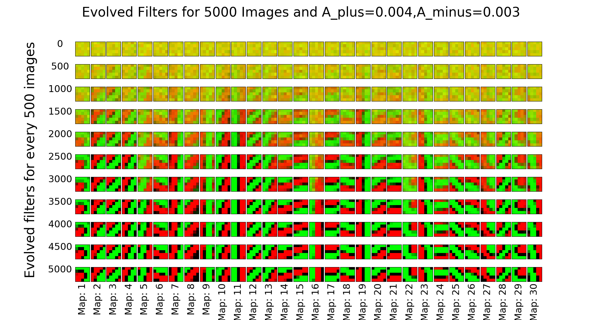
Figure 17: Plot of the weights of 30 maps of L2. The ON (green) $5\times 5$ filter and the OFF (red) $5\times 5$ filter are superimposed on top of each other.

Homeostasis

Homeostasis refers to the convolution kernels (weights) for all maps being updated approximately the same number of times during training. With homeostasis each kernel gets approximately the same number of opportunities to learn its unique feature. Some maps tend to update their weights more than others and, if this continues, these maps can take over the learning. That is, only the features (weights of the convolution filter) of those maps that get updated often will be of value with the rest of the maps not learning any useful feature (as their weights are not updated). Homeostasis was enforced by simply decreasing the weights of a map by $w_{ij}\rightarrow w_{ij}-a^{-}w_{ij}(1-w_{ij})$ if it tries to update more than twice for every 5 of input images.

3.2.2 Pooling Layers

A pooling layer is a way to down sample the spikes from the previous convolution layer to reduce the computational effort.

Max Pooling

After the synapses (convolution kernels or weights) from L1 to L2 have been learned (unsupervised STDP learning is over), they are fixed, but lateral inhibition continues to be enforced in L2. Spikes from the maps of the convolution layer L2 are now passed on to layer L3 using max pooling. First of all, we ignored the last row and last column of each of the $23\times 23$ maps of L2 so that they may be considered to be $22\times 22.$  Next, consider the first map of the convolution layer L2. This map is divided into non-overlapping $2\times 2$ area of neurons. In each of these $2\times 2$ sets of neurons, at most one spike is allowed through. If there is more than one spike coming from the $2\times 2$ area, then one compares the membrane potentials of the spikes and passes the one with the highest membrane potential. Each $2\times 2$ set of neurons in the first map is then a single neuron in the first map of the L3 layer. Thus each map of L3 has $11\times 11$ (down sampled) neurons. This process is repeated for all the maps of L2 to obtain the corresponding maps of L3. Lateral inhibition is not applied in a pooling layer. There is no learning done in the pooling layer, it is just way to decrease the amount of data to reduce the computational effort.

After training the L2 convolution layer, we then passed 60,000 MNIST digits through the network and recorded the spikes from the L3 pooling layer. This is shown in Figure 18. For example, in the upper left-hand corner of Figure 18 is shown the number spikes coming out of the first map of the pooling layer L3 for each of the 10 MNIST digits. It shows that the digit “3” produced over 100, 000 spikes when the 60,000 MNIST digits were passed through the network while the digit “1” produced almost no spikes. That is, the spikes coming from digit “1” do not correlate with the convolution kernel (see the inset) to produce a spike. On the other hand, the digit ”3” almost certainly causes a spike in the first map of the L3 pooling layer. In the bar graphs of Figure 18 the red bars are the five MNIST digits that produced the most spikes in the L3 pooling layer while the blue bars are the five MNIST digits that produced the least.

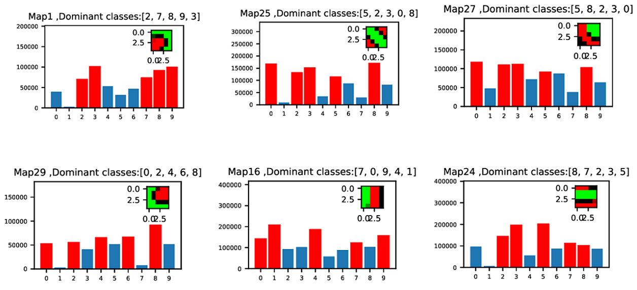
Figure 18: Spikes per map per digit. Headings for each of the sub-plots indicate the dominant (most spiking) digit for respective features.

Figure 19 shows convolution kernel between the L3 pooling layer and the L4 convolution layer. We chose to have 500 maps in L4 which means that for $w=0,1,2,...,499$ we have

$$W_{C2}(w,k,i,j)\in\mathbb{R}^{30\times 5\times 5}\text{ \ for \ }0\leq k\leq 29\text{ \ and }(0,0)\leq(i,j)\leq(4,4).$$

The spikes from the L3 pooling layer are then used to train the weights (convolutional kernels) $W_{C2}$ in the same manner as $W_{C1}.$

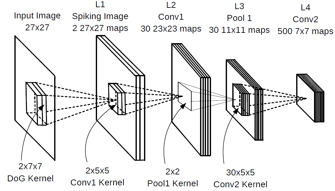
Figure 19: Network showing two convolution layers.

In some of our experiments we simply did a type of global pooling to go to the output layer L5. Specifically, at each time step, we convolve the spikes from L3 to compute the potential for each of the $500\times 7\times 7$ neurons of L4. The maximum potential for each map in L4 was then found and stored (This is a vector in $\mathbb{R}^{500}$). The potentials in L4 were then reset to 0 and the process repeated for each of the remaining time steps of the current image. This procedure results in ten $\mathbb{R}^{500}$ vectors for each image. The sum of these vectors then encodes the current image in L5, i.e., as a single vector in $\mathbb{R}^{500}.$ The motivation to take the maximum potential of each map at each time step is because all the neurons in a given map of L4 are looking for the same feature in the current image.

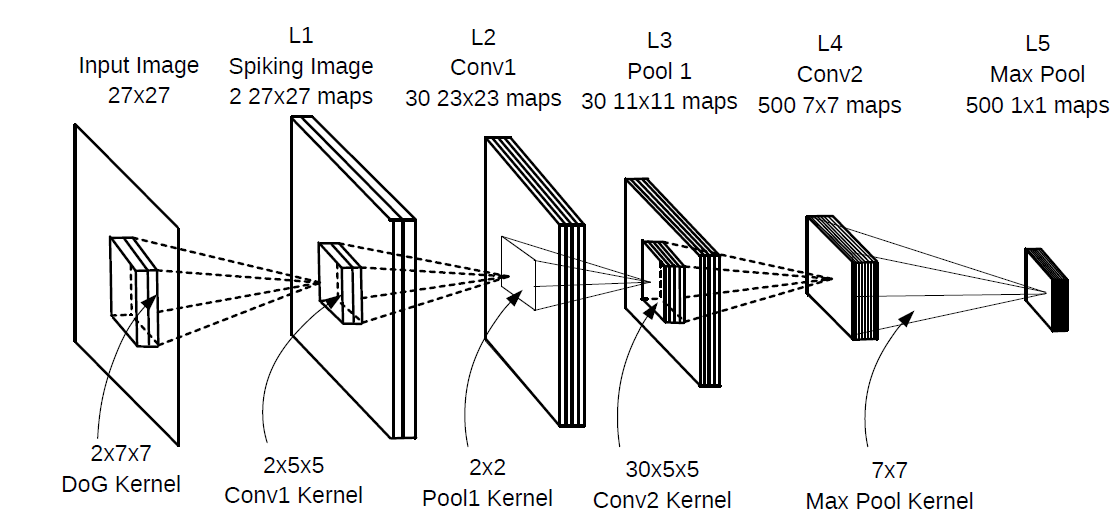
Figure 20: Network with two convolution and pooling layers, global pooling is also shown here.

Unsupervised STDP training is done in the convolution layers with both STDP competition and lateral inhibition applied to the maps of the convolution layer doing training. Once a convolution layer is trained, it’s weights are fixed and the spikes are passed through it with only lateral inhibition imposed.

4 Classification of MNIST data set

In the following subsections we considered two different network architectures along with different classifiers for the MNIST data set.

4.1 Classification with Two Convolution/Pool Layers

In this first experiment the architecture shown in Figure 20 was used. Max pooled ”membrane potentials”, i.e., the L5 layer of Figure 20, was used to transform each $27\times 27$ ($=729)$ training image into a new ”image” in $R^{500}$. Using these images along with their labels, a support vector machine [18] was then used to find the hyperplanes that optimally separate the training digits into 10 classes. With $W\in\mathbb{R}^{45\times 500}$ the SVM weights, the quantity $\lambda W^{T}W$ was added to the SVM Lagrangian to for regularization. Both linear and radial basis function (RBF) kernels were used in the SVM. We used 20,000 MNIST images for the (unsupervised) training of the two convolution/pool layers (Layers L2-L5). Then we used 50,000 images to train the SVM with another 10,000 images used for validation (to determine the choice of $\lambda$). The SVM gives the hyperplanes that optimally separate the 10 classes of digit. Table 1 shows classification accuracies when $500$ maps were used in L4. The first two rows of Table 2 give the test accuracy on 10,000 MNIST test images. In particular, note a 98.01 % accuracy for the RBF SVM and a 97.8 % accuracy for a Linear SVM. Using a similar network with linear SVM, Kheradpisheh et al. [24] reported an accuracy of 98.3%.

Classifier	Test Acc	Valid Acc	Training Time	$\lambda$	$\eta$	Epochs
RBF SVM	97.92 %	97.98 %	8 minutes	1/3.6	-	-
Linear SVM	97.27 %	97.30 %	4 minutes	1/0.012	-	-
2 Layer FCN (backprop)	96.90 %	97.02 %	15 minutes	1.0	$\frac{0.1}{(1.007)^{\#Epoch}}$	30
3 layer FCN (backprop)	97.8 %	97.91 %	50 minutes	6.0	$\frac{0.1}{(1.007)^{\#Epoch}}$	30

Table 1: Classification accuracies on MNIST data set with various classifiers when number of maps in L4 is 500.

For comparison purposes with SVM, we also considered putting the L5 neurons (i.e., vectors in $\mathbb{R}^{500}$) into both a conventional two and three layer fully connected network (FCN). Using a two layer FCN (see Figure 21) with sigmoidal outputs, a cross-entropy cost function, and a learning rate $\eta=0.1/(1.001)^{\#Epoch}$ we obtained 97.97 % classification accuracy. Similarly with a three layer FCN (see Figure 22) with the same conditions an accuracy of 98.01 % was obtained.

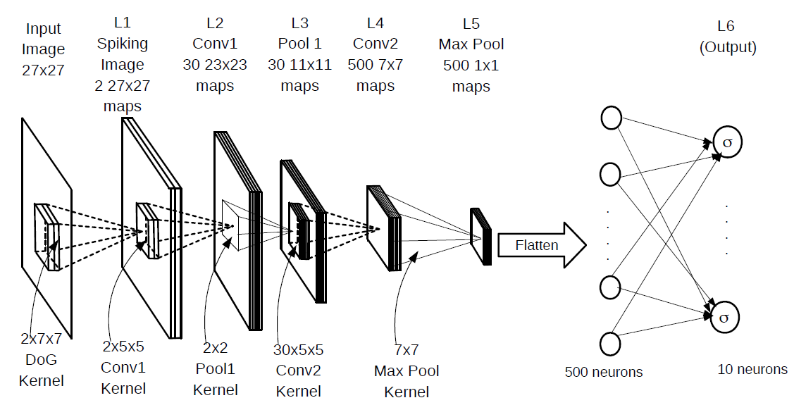
Figure 21: Network showing with 2 fully connected layers as a classifier.

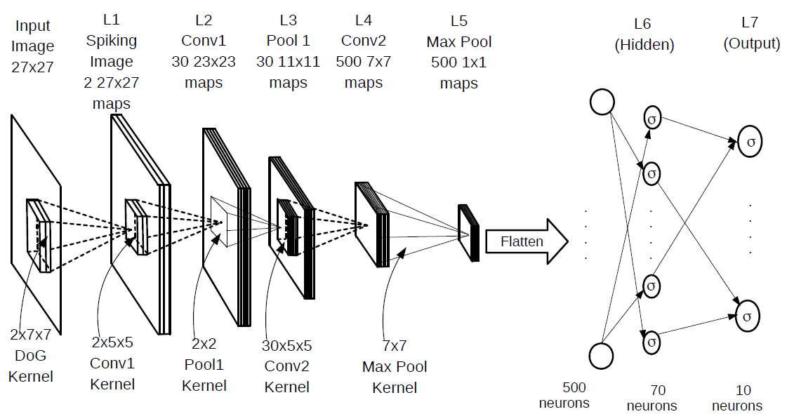
Figure 22: Network showing with 2 fully connected layers as a classifier.

Separability of the MNIST Set

If $\lambda=1/1000$ then the 50,000 training and 10,000 validation images converted to $\mathbb{R}^{500}$ “images” turn out to be completely separable into the 10 digit classes! However, the accuracy on the remaining 10,000 test images drops to 97.01%. The original 60,000 MNIST (training & validation) images in $R^{784}$ are not separable by a linear SVM (The SVM code was run for 16 hours with $\lambda=1/1000$ without achieving separability).

Increasing the Number of Output Maps

If the number of maps in the L4 layer are increased to 1000 with the L5 $1\times 1$ maps correspondingly increased to 1000, then there is a slight increase in test accuracy as shown in Table 2. With $\lambda=1$ the 50,000 training and 10,000 validation images converted to $\mathbb{R}^{1000}$ “images” also turn out to be completely separable into the 10 digit classes. However, with $\lambda=1$ the test accuracy decreases to 97.61.

Classifier	Test Acc	Valid Acc	Training Time	$\lambda$	$\eta$	Epochs
RBF SVM	98.01 %	98.20 %	8 minutes	1/3.6	-	-
Linear SVM	97.80 %	98.02 %	4 minutes	1/0.012	-	-
2 Layer FCN (backprop)	97.71 %	98.74 %	15 minutes	1.0	$\frac{0.1}{(1.007)^{\#Epoch}}$	30
3 layer FCN (backprop)	98.01 %	98.10 %	50 minutes	6.0	$\frac{0.1}{(1.007)^{\#Epoch}}$	30

Table 2: Classification accuracies on MNIST data set with various classifiers when number of maps in L4 is 1000.

4.2 Classification with a Single Convolution/Pool Layer

The architecture shown in Figure 23 has a single convolutional/pooling layer with $30\times 11\times 11=3630$ pooled neurons in L3. These neurons are fully connected to L4 layer of $3630$ neurons. However, the neurons in L4 are in 1-1 correspondence with the L3 neurons (flatten). Further, each neuron in L4 simply sums the spikes coming into it from its corresponding neuron in L3. The L4 neurons are fully connected (with trainable weights) to 10 output neurons. This final layer of weights are then trained using backprop only on this output layer, i.e., only backprop to L4. (See Lee at al. [30] where the error is back propagated through all the layers and reported an accuracy of 99.3%). Inhibition settings are same as in the above experiment.

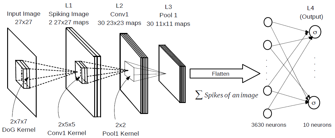
Figure 23: Deep spiking convolutional network architecture for classification of the MNIST data set.

The first row of Table 3 shows a 98.4% test accuracy using back propagation on the output layer (2 Layer FCN). The second and third rows give the classification accuracy using an SVM trained on the L4 neurons (their spike counts). The feature extraction that takes place in the L2 layer (and passed through the pooling layer) results in greater than 98% accuracy with a two layer conventional FCNN output classifier. A conventional FC two layer NN (i.e., no hidden layer) with the $28\times 28$ images of the MNIST data set as input has only been reported to achieve 88% accuracy and 91.6% with preprocessed data [28]. This result strengthens our view that the unsupervised STDP appears to convert the MNIST classes into classes in a higher space that are separable.

We also counted the spikes in network with two convolution/pool layers (see Figure 20) but found that the accuracy decreased (see Table 2) This decrease may be due to that reduced number of spikes in the output neurons compared to have only one convolution/pool layer.

Classifier	Test Acc	Valid Acc	Training Time	$\mathbf{\lambda}$	$\eta$	Epochs
2 Layer FCN	98.4%	98.5%	10mins	$1/10$	$0.1/(1.007)^{\#Epoch}$	20
RBF SVM	98.8%	98.87%	150 minutes	$1/3.6$	-	-
Linear SVM	98.41%	98.31%	100 minutes	$1/0.012$	-	-

Table 3: Classification accuracies on MNIST data set with various classifiers when a single convolution/pool layer is used.

5 Reward Modulated STDP

Reward modulated STDP is a way to use the accumulated spikes at the output to do the final classification (in contrast to SVM and a two layer backprop mentioned above). Figure 24 shows the network architecture where the reward modulated STDP is carried out between the (flattened) L5 layer and the ten output neurons of the L6 layer. The weights between the fully connected neurons of Layer 5 and Layer 6 are then trained as follows: For any input image the spikes through the network arrive between $t=0$ and $t=11$ time steps. The final ($t=11$) membrane potential of the $k^{th}$ output neuron for $k=1,2,...,10$ is then

$$V_{k}=\sum_{t=0}^{11}\sum_{j=1}^{12000}w_{kj}s_{L5}(t,j).$$

Denote by $N_{hit}$ and $N_{miss}$ the number of correctly classified and incorrectly classified images for every $N$ (e.g., $N=100,500,1500,$ etc.) input images so $N_{miss}+N_{hit}=N$. If the $k^{th}$ output potential $V_{k}$ is maximum (i.e., $V_{k}>V_{j}$ for $j\neq k$) and the input image has label $k$ then the weights going into the $k^{th}$ output neuron are rewarded in the sense that

$$w_{kj}\longleftarrow w_{kj}+\Delta w_{kj},\text{ \ where \ }\Delta w_{kj}=\begin{cases}+\dfrac{N_{miss}}{N}a_{r}^{+}w_{kj}(1-w_{kj})\text{ \ if at least one pre-synaptic spike from j to k.}\\ -\dfrac{N_{miss}}{N}a_{r}^{-}w_{kj}(1-w_{kj})\ \ \text{otherwise.}\end{cases}$$ (10)

If $V_{k}$ is the maximum potential, but the label of the image is $j\neq k,$ then the weights going into output neuron $k$ are punished in the sense that

$$w_{kj}\longleftarrow w_{kj}+\Delta w_{kj},\text{ \ where \ }\Delta w_{kj}=\begin{cases}-\dfrac{N_{hit}}{N}a_{p}^{+}w_{kj}(1-w_{kj})\text{ \ if at least one pre-synaptic spike from j to k.}\\ +\dfrac{N_{hit}}{N}a_{p}^{-}w_{kj}(1-w_{kj})\ \ \text{otherwise.}\end{cases}$$ (11)

Note that only the weights of those neurons connected to the output neuron with the maximum potential are updated. The term “modulated” in reward modulated STDP refers to the factors $\dfrac{N_{miss}}{N}$ and $\dfrac{N_{hit}}{N}$ which multiply (modulate) the learning rule. Equation (10) refers to the case where the k^th output neuron also has the high membrane potential of the ten outputs. If $N_{miss}/N$ is small then the network accuracy is performing well in terms of accuracy and the change is weights is small (as the weights are thought to already have learned to correctly classify). On the other hand, equation (11) refers to the case where the k^th output has the highest membrane potential, but the label is $j\neq k.$ Then, if $N_{miss}/N$ is small, it follows that $N_{hit}/N$ is large the weights of the neurons going into the k^th neuron have their values changed by a relatively large amount to (hopefully) correct the misclassification.

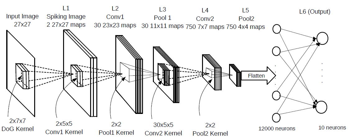
Figure 24: Network with 750 maps in L4.

In this experiment with R-STDP, only 20,000 MNIST digits were used for training, 10,000 digits for validation (used to choose the number of training epochs), and the 40,000 remaining digits were used for testing. The R-STDP synaptic weights between L5 and L6 were initialized from the normal distribution $\mathcal{N}(0.8,0.01)$. Table 4 shows that a test accuracy of only 90.1% was obtained.

Maps in L4	Valid acc %	Test Acc %	Epochs
750	91.2	90.1	150

Table 4: Classification accuracy on MNIST data set with R-STDP when one neuron per class is used.

For comparison, we replaced the R-STDP classifier (from L5 to L6) with a simple 2 layer neural network (from L5 to L6) which used error back propagation. These weights for back propagation were initialized from the normal distribution $\mathcal{N}(0,1/\sqrt{12000})$ as in [45]. Table 6 shows that R-STDP performed poorly compared to the simple two layer backprop which ran for only 20 epochs.

Classifier	Test Acc	Valid Acc	$\mathbf{\lambda}$	$\eta$	Epochs
2 Layer FCN	97.5%	97.6%	$1.0$	$0.1/(1.007)^{\#Epoch}$	20

Table 5: Classification accuracy on MNIST data set with single layer backprop.

Mozafari et al. [42][41] got around this poor performance by having 250 neurons in the output layer and assigning 25 output neurons per class. They reported 97.2 % test accuracy while training on 60,000 images and testing on 10,000 images. We also considered multiple neurons per class in the output layer. As Table 6 shows, we considered 300 output neurons (30 per class) and we also consider dropout. $P_{drop}=0.4$ means that $0.4(300)=120$ output neurons were prevented from updating their weights for the particular training image. For each input image a different set of 120 randomly neurons were chosen to not have their weights updated. Table 6 shows that the best performance of 95.91 % test accuracy was obtained with $P_{drop}=0.4.$

Maps in L4	#Output Neurons	Pdrop	Valid acc %	Test acc %	Epochs
750	300	0.3	95.81	95.84	400
750	300	0.4	96.01	95.91	400
750	300	0.5	95.76	95.63	400

Table 6: Classification accuracy on MNIST data set with R-STDP when more than one neuron per class is used.

5.1 R-STDP as a Classification Criteria

We experimented with R-STDP learning rule applied to L5-L6 synapses of the network in the Figure 24 by two different kinds of weight initialization and also varying initialization of parameters like $\dfrac{N_{miss}}{N},$ $\dfrac{N_{hit}}{N}$ and $N$.

5.1.1 Backprop Initialized Weights for R-STDP

We were concerned with the poor performance using an R-STDP as a classifier as given in Table 6. In particular, perhaps the weight initialization plays a role in that the R-STDP rule can get stuck in a local minimum. To study this in more detail the network in Figure 24 was initialized with a set of weight that are known to give a high accuracy. To explain, the final weights used in the 2 Layer FCN reported in Table 5 were used as a starting point. As these weights are both positive and negative, they were shifted to be all positive. This was done by first finding the minimum value $w_{\min}$ $(<0)$ of these weights and simply adding $-w_{\min}>0$ to them so that they are all positive. Then this new set of weights were re-scaled to be between 0 and 1 by dividing them all by their maximum value (positive). These shifted and scaled weights were then used to initialize the weights of the R-STDP classifier. The parameters $a_{r}^{+},a_{r}^{-},a_{p}^{+},a_{p}^{-}$ were initialized to be 0.004, 0.003, 0.0005, 0.004 respectively. With the network in Figure 24 initialized by these weights, the validation images were fed through the network and the neuron number with the maximum potential is the predicted output. The validation accuracy was found to be 97.1%.

With weights of the fully connected layer of Figure 24 initialized as just described, the R-STDP rule was used to train the network further for various number of epochs and two different ways of updating $\dfrac{N_{miss}}{N}$ and $\dfrac{N_{hit}}{N}.$

Batch Update of $\dfrac{N_{miss}}{N}$ and $\dfrac{N_{hit}}{N}$

The first set of experiments were done with the $\dfrac{N_{miss}}{N}$ and $\dfrac{N_{hit}}{N}$ ratios updated after every batch of $N$ images for $N=100,500,1500,2500.$ As the weights of the fully connected layer of Figure 24 with the backprop trained values, we expect $\dfrac{N_{miss}}{N}$ to be a low fraction or equivalently $\dfrac{N_{hit}}{N}$ to be high. Consequently, they were initialized as $\dfrac{N_{miss}}{N}=0.1,$ $\dfrac{N_{hit}}{N}=0.9.$ With these initialization, Table 7 shows that accuracy on the validation set did not decrease significantly for $N$ not too large. However, using larger values of $N$ (value of N depends on the initialization of $N_{miss}/N$ and $N_{hit}/N$) the accuracy goes down significantly. For example, for the cases where $N_{miss}/N=0.035$ and $N_{hit}/N=0.965$ the accuracy didn’t significantly decrease until the batch size was $N=3500.$ In the case with $N_{miss}/N=0.0$ and $N_{hit}/N=1.0$ the accuracy didn’t decrease at all. This is because the best performing weights for validation accuracy were used, but these same weights also gave 100% accuracy on the training data.

$\dfrac{N_{miss}}{N}$	$\dfrac{N_{hit}}{N}$	$N$	Acc. at start	Acc. at end
0.1	0.9	100	97.1%	96.91%
0.1	0.9	500	97.1%	96.96%
0.1	0.9	1500	97.1%	96.82%
0.1	0.9	2500	97.1%	90.76%
0.035	0.965	2500	97.1%	96.69%
0.035	0.965	3000	97.1%	96.58%
0.035	0.965	3500	97.1%	91.05%
0.035	0.965	4000	97.1%	90.98%
0.0	1.0	100	97.1%	96.93%
0.0	1.0	500	97.1%	96.93%
0.0	1.0	1500	97.1%	96.94%
0.0	1.0	2500	97.1%	96.94%
0.0	1.0	3000	97.1%	96.94%
0.0	1.0	3500	97.1%	96.94%
0.0	1.0	4000	97.1%	96.93%

Table 7: Demonstration of sensitivity of R-STDP to N value with correct initialization of hit and miss ratios.

Table 8 shows the classification accuracy with ”poor” initialization $N_{miss}/N=0.9$ and $N_{hit}/N=0.1.$ If the weights had been randomly initialized then the initialization $N_{miss}/N=0.9$ and $N_{hit}/N=0.1$ would be appropriate. However, Table 8 shows that R-STDP isn’t able to recover from this poor initialization.

$\dfrac{N_{miss}}{N}$	$\dfrac{N_{hit}}{N}$	$N$	Acc. at start	Acc. at end
0.9	0.1	100	97.1%	91.52%
0.9	0.1	500	97.1%	90.67%
0.9	0.1	1500	97.1%	90.47%
0.9	0.1	2500	97.1%	90.45%

Table 8: Demonstration of sensitivity of R-STDP to N value with incorrect initialization of hit and miss ratios.

Update of $\dfrac{N_{miss}}{N}$ and $\dfrac{N_{hit}}{N}$ after each image

Next, $N_{miss}/N$ and $N_{hit}/N$ were updated after every image using the most recent $N$ images. Even with $N_{miss}/N$ and $N_{hit}/N$ initialized incorrectly, the validation accuracies in Table 9 did not decrease significantly. Though the accuracy still goes down slightly, the table indicates that updating $N_{miss}/N$ and $N_{hit}/N$ after every image mitigates this problem.

$\dfrac{N_{miss}}{N}$	$\dfrac{N_{hit}}{N}$	$N$	Acc. at start	Acc. at end
0.9	0.1	100	97.1%	96.93%
0.9	0.1	500	97.1%	96.94%
0.9	0.1	1500	97.1%	96.93%
0.9	0.1	2500	97.1%	96.94%

Table 9: Demonstration of sensitivity of R-STDP.

Still updating $N_{miss}/N$ and $N_{hit}/N$ after each image, it was found that R-STDP accuracy was very sensitive to the initialized weights. Specifically the L5-L6 R-STDP weights were initialized using the backprop trained weights (as explained above) by doing the backprop for just 10 epochs (instead of 20) and $\lambda=10.0$ (regularization parameter) which gave 99.6% training and 96.8% validation accuracies. Table 10 gives the validation accuracies using R-STDP for 100 epochs. Surprisingly, even with a good initialization of the weights and the ratios $N_{miss}/N$ and $N_{hit}/N$, the validation accuracy suffers.

$\dfrac{N_{miss}}{N}$	$\dfrac{N_{hit}}{N}$	$N$	Acc. at start	Acc. at end
0.0	1.0	100	96.8%	90.75%
0.0	1.0	4000	96.8%	90.67%

Table 10: Demonstration of sensitivity of R-STDP for weight initialization.

For this same cases as Table 10, the R-STDP algorithm was run for 1000 epochs with the training and validation accuracies versus epoch plotted in Figure 25. Notice that the validation accuracy drops to ~90%. It seems that R-STDP is not a valid cost function as far as accuracy is concerned. Interestingly, as shown next, training with R-STDP with randomly initialized weights, the validation accuracy only goes up to ~90% (see Figure 26).

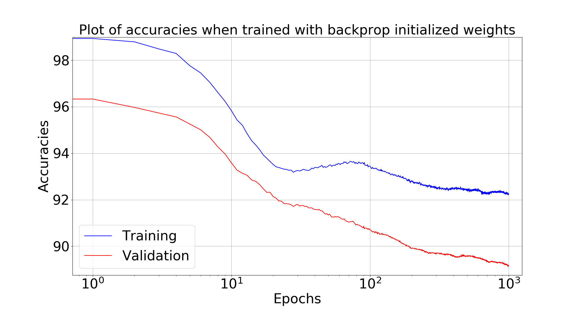
Figure 25: Plot of accuracies versus epochs when the weights were initialized with backprop trained weights.

5.1.2 Randomly Initialized Weights for R-STDP

In the set of experiments, the weights trained with R-STDP were randomly initialized from the normal distribution $\mathcal{N}(0.8,0.01)$ and the $N_{miss}/N,N_{hit}/N,N$ parameters initialized with the values given in Table 13. Validation accuracies are shown at the end of 100 epochs $N_{miss}/N$ and $N_{hit}/N,N$ were updated after every image.

$\dfrac{N_{miss}}{N}$	$\dfrac{N_{hit}}{N}$	$N$	Acc. at start	Acc. at end
0.9	0.1	100	10.3	90.22
0.9	0.1	500	10.1	90.13
0.9	0.1	1500	10.2	90.12
0.9	0.1	2500	10.6	90.16

Table 11: Demonstration of sensitivity of R-STDP.

For this same cases as Table 11, the R-STDP algorithm was run for 1000 epochs with the training and validation accuracies versus epoch plotted in Figure 26. The validation accuracy only goes up to ~90%.

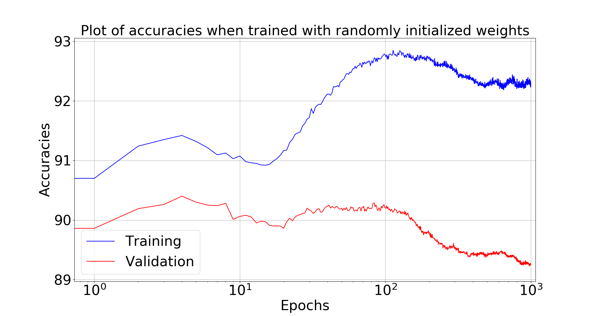
Figure 26: Plot of accuracies versus epochs when the weights were randomly initialized.

6 Classification of N-MNIST data set

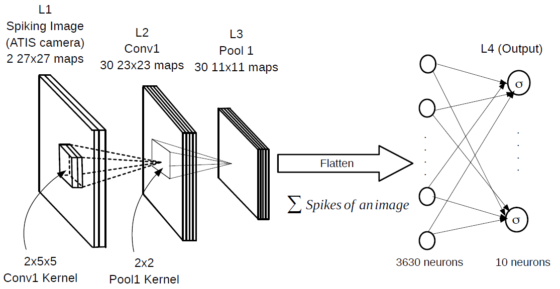
Figure 27: Network for N-MNIST classification.

In the above we artificially constructed spiking images using a DoG filter on the standard MNIST data set as in [24][23]. However the ATIS (silicon retina) camera [49] works by producing spikes. We also considered classification directly on recorded output from the ATIS camera given in the N-MNIST data set [46]. A silicon retinal detects change in pixel intensity and thus the MNIST digits are recorded with camera moving slightly (saccades). Figure 28 shows the raw accumulated spikes of the N-MNIST data set as given in [46].

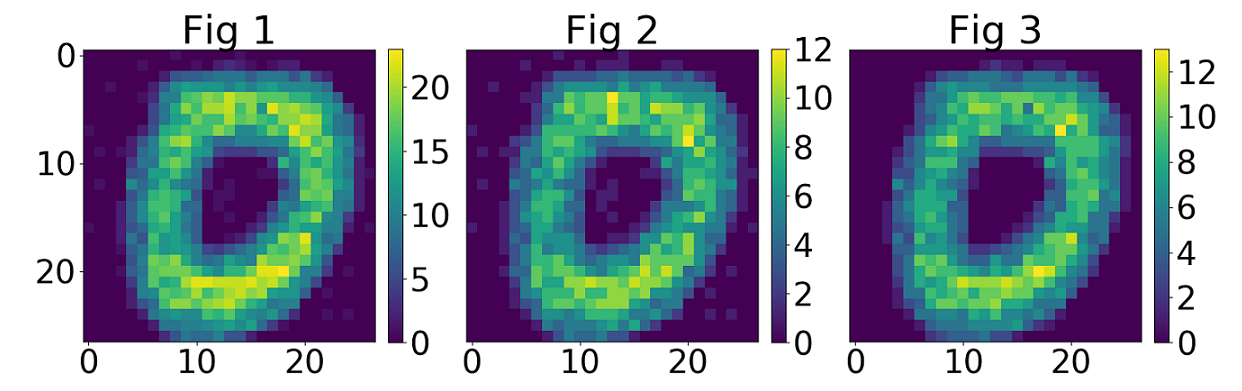
Figure 28: Left: Accumulated ON and OFF center spikes. Center: Accumulate ON center spikes. Right: Accumulated OFF center spikes.

Figure 29 is the same as Figure 28, but corrected for saccades (camera motion) using the algorithm given in [46].

Figure 29: Left: Accumulated ON and OFF center spikes. Center: Accumulate ON center spikes. Right: Accumulated OFF center spikes.

Figure 27 shows the network we used for classification of the N-MNIST data. We first hard wired the weights $W_{C1}$ of the convolution kernel from L1 to L2 of Figure 27 to the values already trained above in subsection 4.2 (see Figure 23). Only the weights from L4 to L5 were trained for classification by simply back propagating the errors from L5 to L4. This result in given in the first row of Table 12. We also trained an SVM on the L4 neuron outputs with the results given in row 2 (RBF) and row 3 (linear) of Table 12. All the results in Table 12 were done on the raw spiking inputs from [46] (i.e., not corrected for saccade) with training done on 50,000 (spiking) images, validation & testing done on 10,000 images each.

Classifier	Test Acc	Valid Acc	Training Time	$\mathbf{\lambda}$	$\eta$	Epochs
2 Layer FCN	97.45%	97.62%	5 minutes	$\frac{1}{10.0}$	$\frac{0.1}{1.007^{\#Epoch}}$	20
RBF SVM	98.32%	98.40%	200 minutes	$\frac{1}{3.6}$	-	-
Linear SVM	97.64%	97.71%	100 minutes	$\frac{1}{0.012}$	-	-

Table 12: Classification accuracies of N-MNIST data set with one convolution/pool layers for transfer learning.

In Table 13 we show the results for the case where the weights $W_{C1}$ of the convolution kernel from L1 to L2 of Figure 27 were trained (unsupervised) using the N-MNIST data set. In this instance we used N-MNIST data corrected for saccades since this gave better result than the uncorrected data. All the results in Table 8 were produced by training on 50,000 (spiking) images with validation & testing done using 10,000 images each.

Classifier	Test Acc	Valid Acc	Training Time	$\mathbf{\lambda}$	$\eta$	Epochs
1 Layer FCN	97.21%	97.46%	5 minutes	$\frac{1}{10.0}$	$\frac{0.1}{1.007^{\#Epoch}}$	20
RBF SVM	98.16%	98.2%	150 minutes	$\frac{1}{3.6}$	-	-
Linear SVM	97.38%	97.44%	100 minutes	$\frac{1}{0.012}$	-	-

Table 13: Classification accuracies of N-MNIST data set with one convolution/pool layers when trained with N-MNIST spikes.

We also added an extra convolution layer, but found that the classification accuracy decreased. Jin et al reported an accuracy of 98.84% by using a modification of error back propagation (all layers) algorithm [21]. Stromatias et al reported an accuracy of 97.23% accuracy by using artificially generated features for the kernels of the first convolutional layer and training a 3 layer fully connected neural network classifier on spikes collected at the first pooling layer [58].

7 Catastrophic Forgetting

Catastrophic forgetting is a problematic issue in deep convolutional neural networks. In the context of the MNIST data set this refers to training the network to learn the digits 0,1,2,3,4 and, after this is done, training on the digits 5,6,7,8,9 is carried on. The catastrophic part refers to the problem that the network is no longer able to classify the first set of digits 0,1,2,3,4. In more detail, Figure 30 shows a conventional (non-spiking) neural network with one convolution layer & one pool layer followed by a fully connected softmax output.

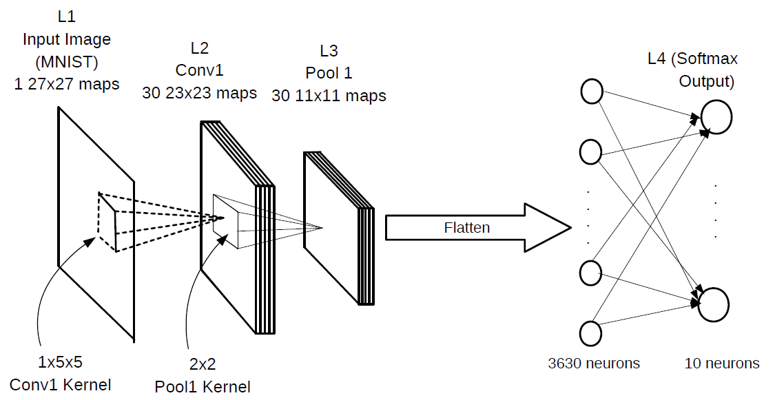
Figure 30: Network architecture for catastrophic forgetting.

This network has 10 outputs but was first trained only on the digits 0,1,2,3,4 back propagating the error (computed from all 10 outputs) to the input (convolution) layer. This training used approximately 2000 digits per class and was done for 75 epochs. Before training the network on the digits 5,6,7,8,9 we initialized the weights and biases of the convolution and fully connected layer with the saved weights of the previous training. For the training with the digits 5,6,7,8,9 we fixed the weights and biases of the convolution layer with their initial values. The network was then trained, but only the weights of fully connected layer were updated. (I.e., the error was only back propagated from the 10 output neurons to the previous layer (flattened pooled neurons). This training also used approximately 2000 digits per class and was done for 75 epochs. While the network was being trained on the second set of digits, we computed the validation accuracy on all 10 digits at the end of each epochs. We plotted these accuracies in Figure 31. The solid red line in Figure 31 are the accuracies versus epoch on the first set of digits {0,1,2,3,4} while the solid blue line gives the accuracies on the second set of digits {5,6,7,8,9} versus epoch. Figure 32 is a zoomed in picture of Figure 31 for better resolutions of the accuracies above 90%. These plots also show the validation accuracy results when the second set of training data modified to include a fraction of data from the first set of training digits {0,1,2,3,4}. For example, the dashed red line is the validation accuracy on the first set of digits when the network was trained with 2000 digits per class of {5,6,7,8,9} along with 200 (10%) digits per class of {0,1,2,3,4}. The blue dashed line is the validation accuracy of the second set of digits after each epoch. Similarly this was done with 15%, 25%, 27.5%, and 30% of the first set of digits included in the training set of the second set of digits. The solid red line shows that after training with the second set of digits for a single epoch the validation accuracy on first set goes down to 10% (random accuracy). The solid blue line shows a validation accuracy of over 97% on the second set of digits after the first epoch. Thus the network has now learned the second set of digits but has catastrophically forgotten the first set of digits shown by solid red line.

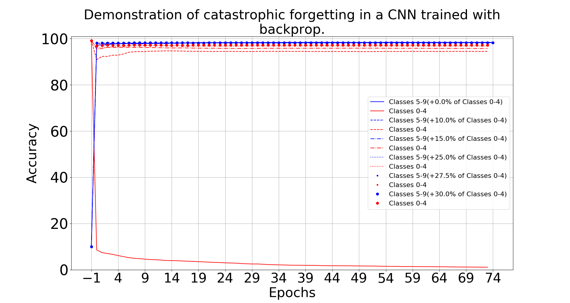
Figure 31: Catastrophic forgetting in a convolutional network while revising a fraction of the previously trained classes. Note that epoch -1 indicates that the network was tested for validation accuracy before training of the classes 5-9 started. Brackets in the legend shows the fraction of previously trained classes that were used to revise the weights from the previous classes.

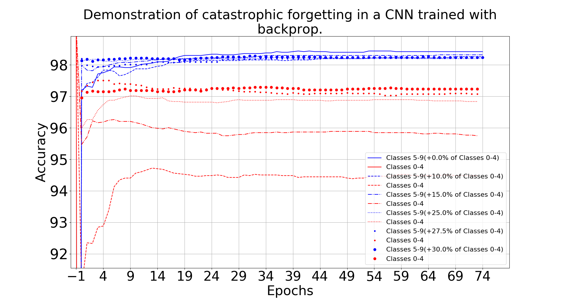
Figure 32: Zoomed upper portion of the Figure 31

7.1 Forgetting In Spiking Networks

For comparison we tested forgetting in our spiking network of Section 4.2 (see Figure 23). The network was first trained only on the digits 0,1,2,3,4 with STDP on the convolution layer and back propagating the error (computed from all 10 outputs) just to the previous (flattened pool layer) layer. This training used approximately 2000 digits per class and was done for 75 epochs. Then, before training the network on the set of digits {5,6,7,8,9}, we initialized the weights of the convolution and fully connected layer with the saved weights of the previous training. For the training with the digits 5,6,7,8,9 we fixed the weights of the convolution layer with their initial values. The network was then trained, but only the weights of fully connected layer were updated. (I.e., the error was only back propagated from the 10 output neurons to the previous layer (flattened pooled neurons). This training also used approximately 2000 digits per class and was done for 75 epochs. While the network was being trained on the second set of digits, we computed the validation accuracy on all 10 digits at the end of each epochs. We plotted these accuracies in Figure 33. The solid red line in Figure 33 are the accuracies versus epoch on the first set of digits {0,1,2,3,4} while the solid blue line gives the accuracies on the second set of digits {5,6,7,8,9} versus epoch. Figure 34 is a zoomed in picture of Figure 33 for better resolutions of the accuracies above 90%. These plots also show the validation accuracy results when the second set of training data modified to include a fraction of data from the first set of training digits {0,1,2,3,4}. For example, the dashed red line is the validation accuracy on the first set of digits when the network was trained with 2000 digits per class of {5,6,7,8,9} along with 200 (10%) digits per class of {0,1,2,3,4}. The blue dashed line is the validation accuracy of the second set of digits after each epoch. Similarly this was done with 15%, 25%, 27.5%, and 30% of the first set of digits included in the training set of the second set of digits. The solid red line shows that after training with the second set of digits for a single epoch the validation accuracy on first set goes down to 77% (compared to the 10% accuracy of a non-spiking CNN). The solid blue line shows a validation accuracy of about 95% on the second set of digits after the first epoch. Thus the network has now learned the second set of digits but has not catastrophically forgotten the first set of digits shown by solid red line.

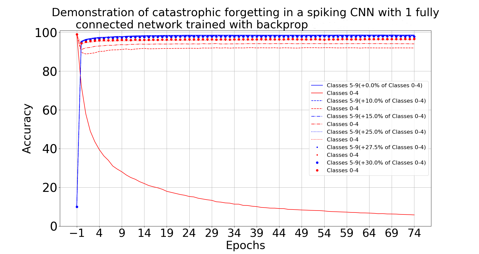
Figure 33: Catastrophic forgetting in a spiking convolutional network while revising a fraction of the previously trained classes. Note that epoch -1 indicates that the network was tested for validation accuracy before training of the classes 5-9 started. Brackets in the legend shows the fraction of previously trained classes that were used to revise the weights from the previous classes.

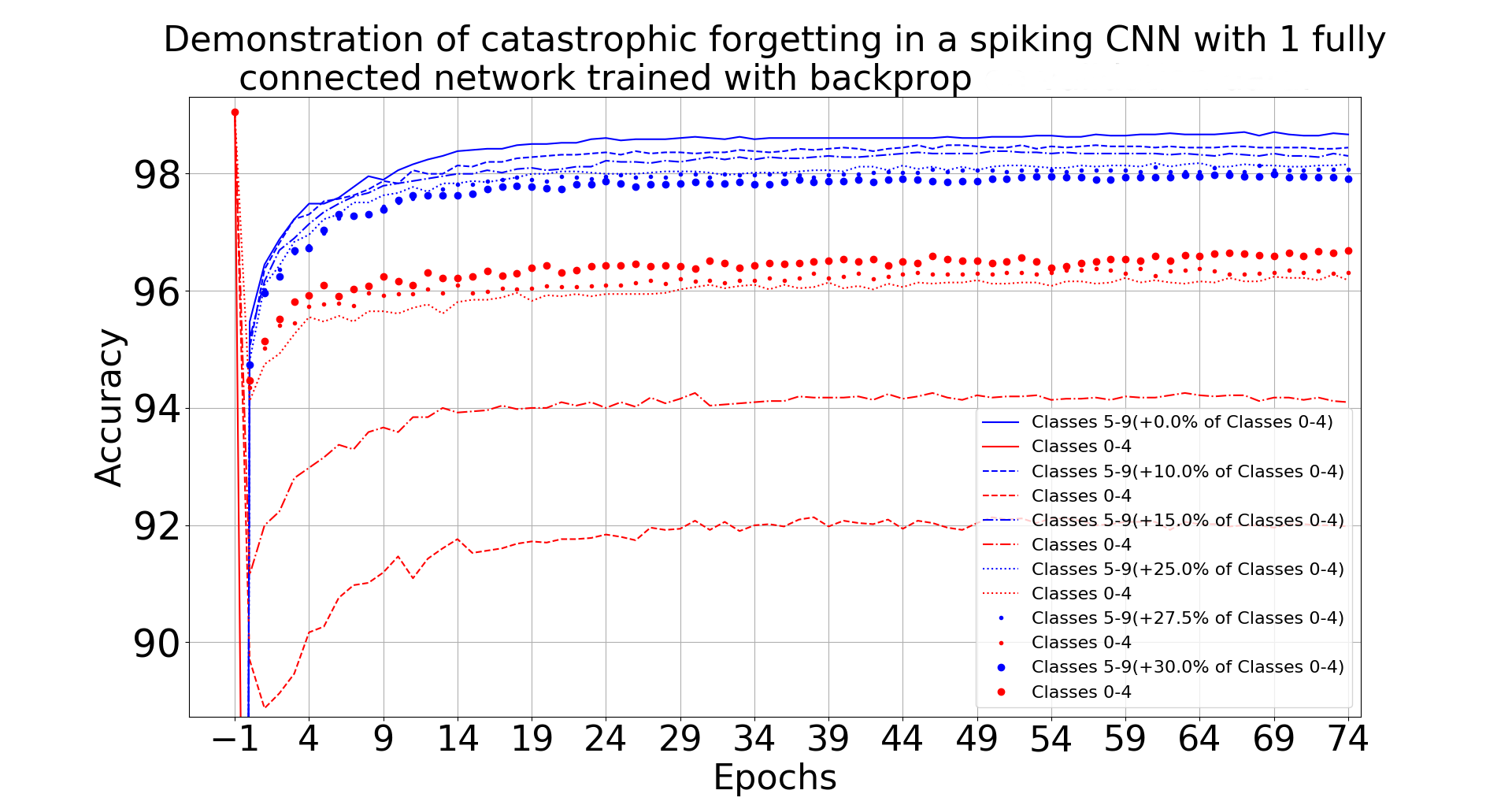
Figure 34: Zoomed upper portion of the Figure 33

As another approach we first trained on the set {0,1,2,3,4} exactly as just describe above. However, we then took a different approach to training on the set {5,6,7,8,9}. Specifically we trained on 500 random digits chosen from {5,6,7,8,9} (approximately 50 from each class) and then compute the validation accuracy on all ten digits. We repeated this for every additional 250 images with the results shown in Figure 35. Interestingly this shows that if we stop after training on 1000 digits from {5,6,7,8,9} we retain a validation accuracy of 91.1%  and 90.71% test accuracy on all 10 digits.

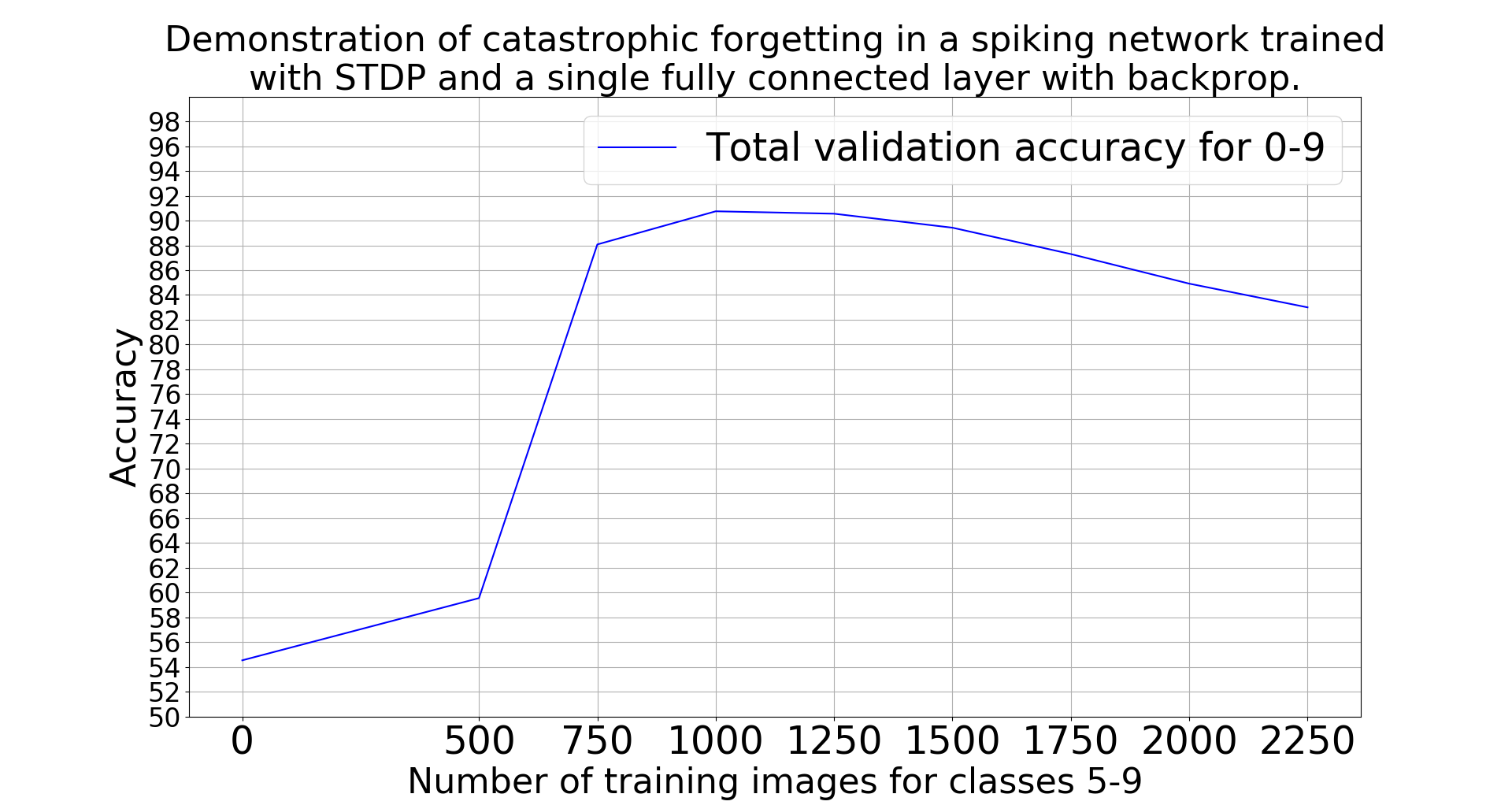
Figure 35: Note that as the number of training images for the classes 5-9 increases the total accuracy drops.

# images (classes 5-9)	# images (classes 0-4)	Validation	Test	Epochs
10,000	1000(10%)	95.235%	95.1%	75
10,000	1500(15%)	95.95%	95.9%	75
10,000	2500(25%)	96.83%	96.81%	75
10,000	2750(27.5%)	96.98%	96.92%	75
10,000	3000(30%)	97.1%	97.043%	75

Table 14: Demonstration of forgetting in a spiking convolution network.

Jason et al reported an accuracy of 93.88% for completely disjoint data sets[1].

8 Feature Reconstruction

We have already presented in Figure 17 which is a reconstruction of the convolution kernels (weights) from Layer L1 to Layer 2 into features. Each of the 30 maps of L2 has a convolution kernel in $\mathbb{R}^{2\times 5\times 5}$ associated with it which maps L1 to L2.

We now want to reconstruct (visualize) the features learned by the second convolution layer. Each of the 500 maps of L4 (see Figure 19) has a convolutional kernel in associated with it which maps L3 to L4, i.e., for $w=0,1,2,...,499$ we have

$$W_{C2}(w,k,i,j)\in\mathbb{R}^{30\times 5\times 5}\text{ \ for \ }0\leq k\leq 29\text{ \ and }(0,0)\leq(i,j)\leq(4,4).$$

A $5\times 5$ area of pooled layer L3 receives spikes from $10\times 10$ area of neurons in L2. Thus, for $w=0,1,2,...,499$, the kernels $W_{C2}(w,k,i,j)\in\mathbb{R}^{30\times 5\times 5}$ are reconstructed to be features

$$F_{P1}(w,k,i,j)\in\mathbb{R}^{30\times 10\times 10}\text{\ \ for \ }0\leq k\leq 29\text{ \ and }(0,0)\leq(i,j)\leq(9,9)$$

connecting L2 to L4. How is this done? Consider the $0^{th}$ kernel $W_{C2}(0,k,i,j)$ and for the $k^{th}$ $5\times 5$ slice of $W_{C2}(0,k,i,j)\in\mathbb{R}^{30\times 5\times 5}$ the value of the $(i,j)$ element is mapped to the $(2i,2j)$ element of the $k^{th}$ $10\times 10$ slice of $F_{P1}(0,k,i,j)\in\mathbb{R}^{30\times 10\times 10}.$ All other values of the $k^{th}$ $10\times 10$ slice are set to zero. This is done for $w=0,1,...,499.$

Now recall that there are 30 kernels in $W_{C1}$. Specifically, for $z=0,1,2,...,29,$

$$W_{C1}(z,k,i,j)\in\mathbb{R}^{2\times 5\times 5}\text{ \ for \ }0\leq k\leq 1\text{ \ and }(0,0)\leq(i,j)\leq(4,4).$$

$k=0$ is for ON center kernels and $k=1$ is for off center kernels. These $W_{C1}$ kernels maps spikes from $14\times 14$ area of neurons in L1 to a $10\times 10$ area of layer of L2. Thus the feature $F_{P1}(0,k,i,j)\in\mathbb{R}^{30\times 10\times 10}$ must be reconstructed to be a feature in $\mathbb{R}^{2\times 14\times 14}$. That is, for $k=0,1$

$$F_{L1}(w,k,i,j)\in\mathbb{R}^{2\times 14\times 14}$$

(Each neuron in L4 has a field of view of $2\times 14\times 14$ neurons in L1). How is this done?

Let the $5\times 5$ matrix on the left-hand side of Figure 36 denote an ON center kernel $W_{C1}(z,0,i,j)\in\mathbb{R}^{5\times 5}$ for some $z=0,1,...,29.$ In particular, let it be the second kernel so $z=1.$ Now the $0^{th}$ feature denoted by $F_{P1}(0,k,i,j)\in\mathbb{R}^{30\times 10\times 10}$ can be visualized as being made up of $10\times 10$ slices for $k=0,1,...,29.$ To go with the second kernel $W_{C1}(1,0,i,j)\in\mathbb{R}^{5\times 5}$ we take the second slice (k=1) of the feature $F_{P1}(0,k,i,j)\in\mathbb{R}^{30\times 10\times 10}$ denoted as $F_{P1}(0,1,i,j)\in\mathbb{R}^{10\times 10}$ which we take to be the $10\times 10$ matrix on the right-hand side of Figure 36. In practice these slices are sparse and we show the particular slice Figure 36 to have only two non zero elements, the $(1,1)$ and the $(5,5)$ elements.

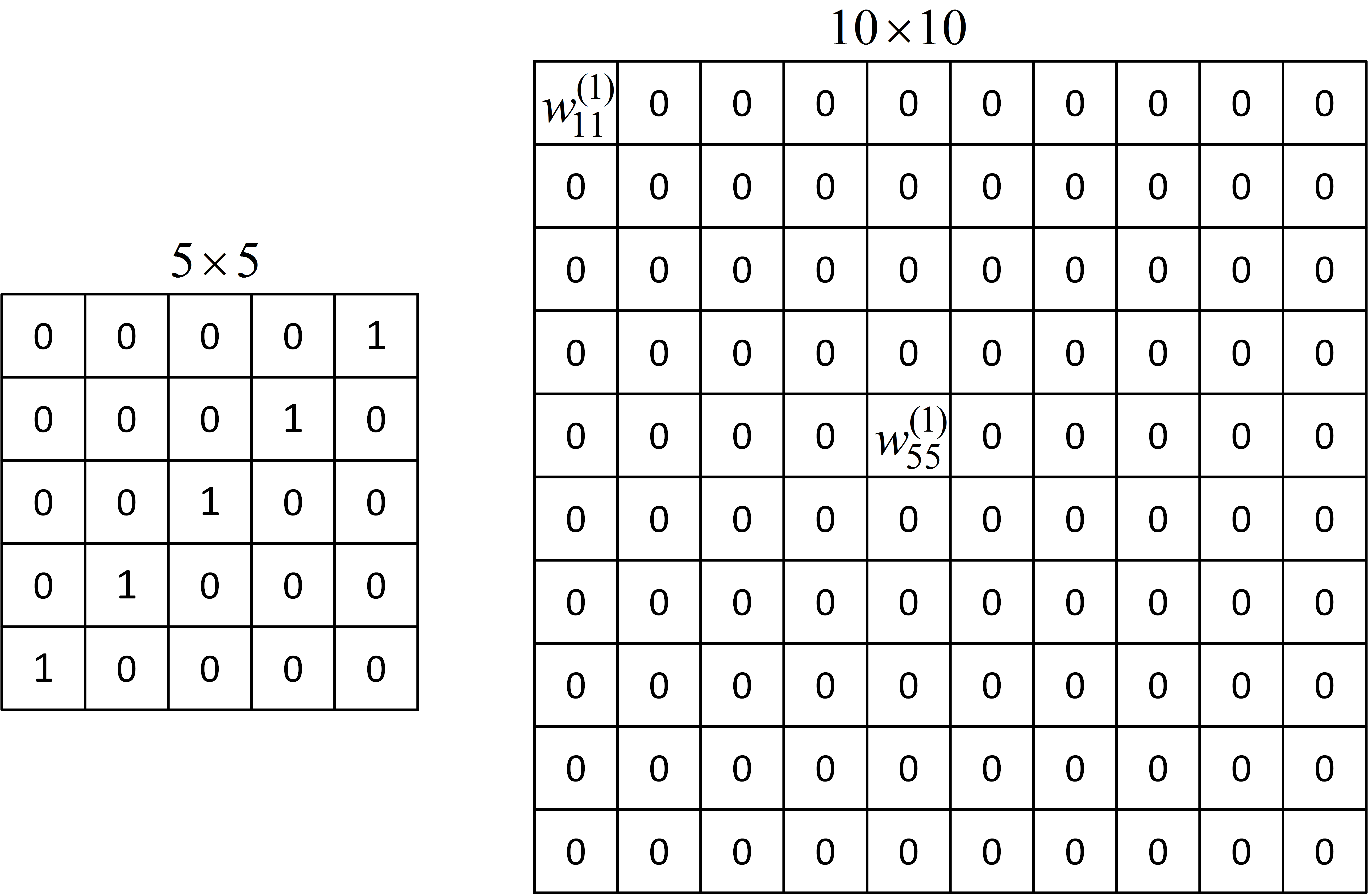
Figure 36: Left: First ON $5\times 5$ slice. Right: First $10\times 10$ slice of pool 1 features.

To carry out the reconstruction we compute $w_{11}^{(1)}W_{C1}(1,0,i,j)\in\mathbb{R}^{5\times 5}$ and center it on $w_{11}^{(1)}$ of $F_{P1}(0,1,i,j)\in\mathbb{R}^{10\times 10}$ as indicated in Figure 37. We then repeat this process for all non zero elements of $F_{P1}(0,1,i,j)\in\mathbb{R}^{10\times 10}$ which in this example is just $w_{55}^{(1)}$.

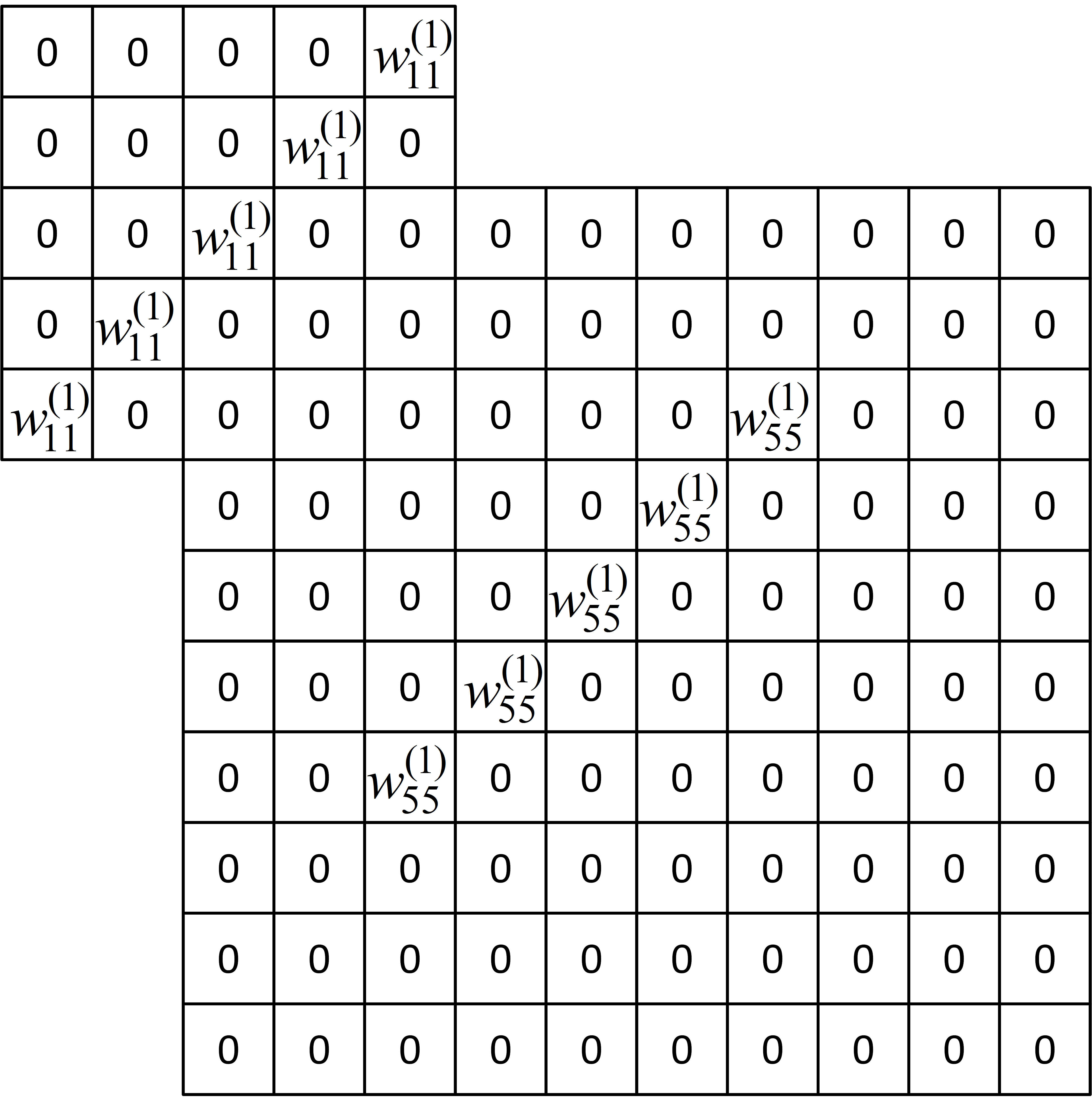
Figure 37: Reconstruction at Conv1 (L2)

Filling in with zeros we end up with the $14\times 14$ matrix shown in Figure 38.

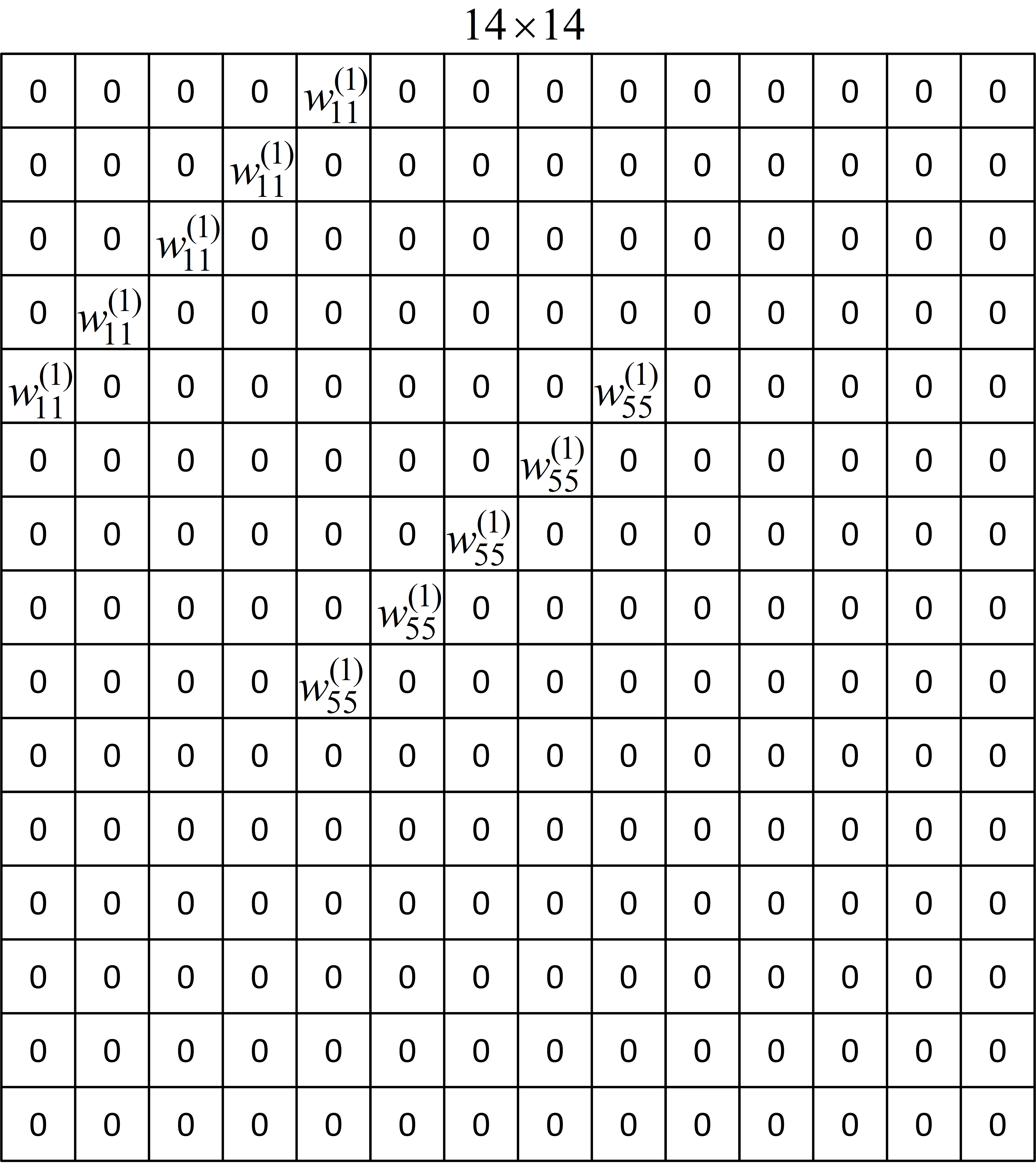
Figure 38: Reconstruction at Conv1 (L2)

Each of the 500 reconstructed features of which 150 are shown in Figure 42 is the sum of 30 $14\times 14$ matrices of the type shown in Figure 38.

To reconstruct the third $14\times 14$ matrix we use the third kernel $W_{C1}(2,0,i,j)\in\mathbb{R}^{5\times 5}$ ($z=2$) taken to be the $5\times 5$ matrix on the left-side of Figure 39 and the third slice ($k=2$) of the feature $F_{P1}(0,k,i,j)\in\mathbb{R}^{30\times 10\times 10}$ denoted as $F_{P1}(0,2,i,j)\in\mathbb{R}^{10\times 10}$ which we take to be the $10\times 10$ matrix on the right-hand side of Figure 39.

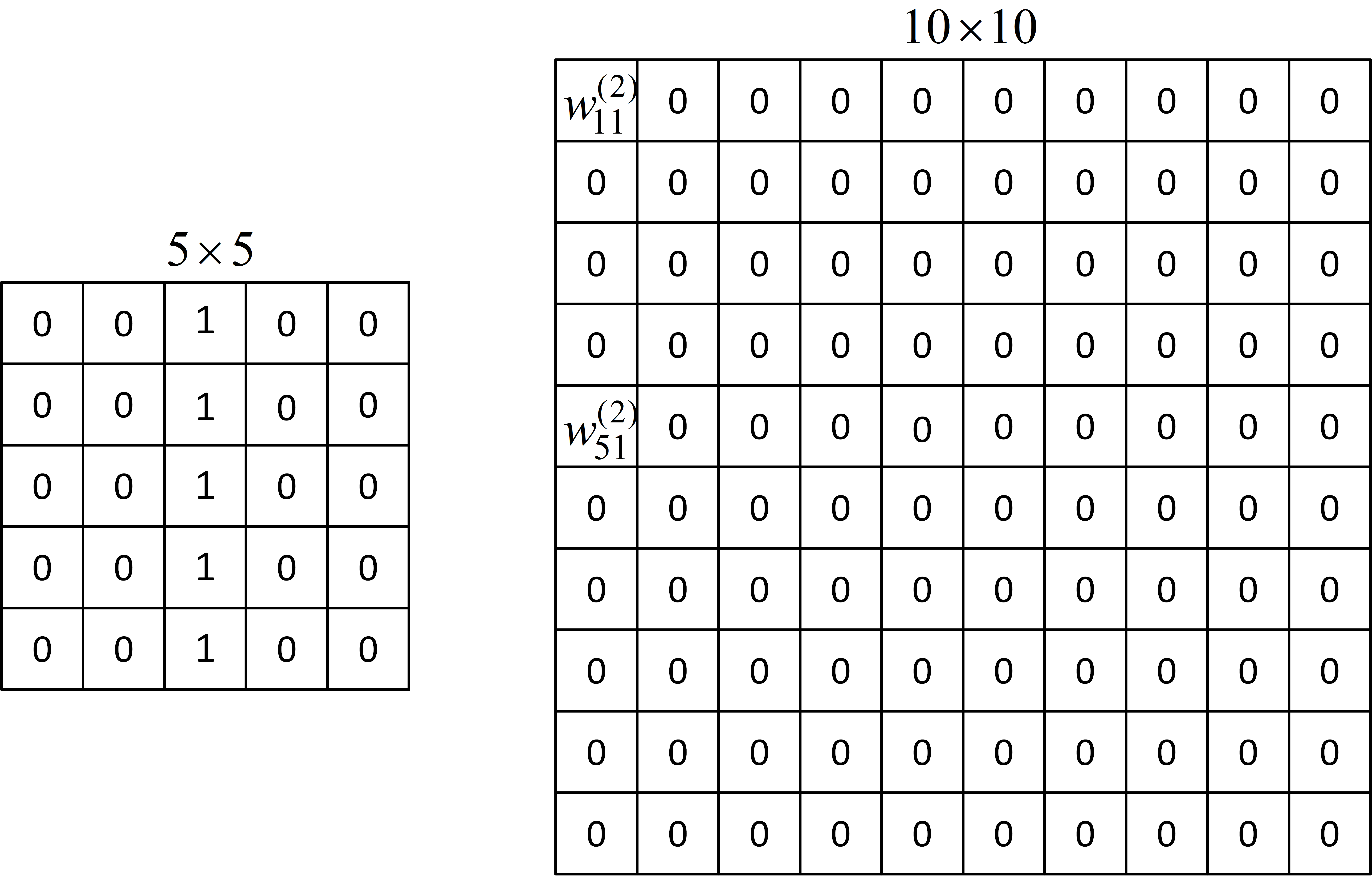
Figure 39: Left: Second ON $5\times 5$ slice. Right: Second $10\times 10$ slice of pool 1 features.

Here the only non zero components are $w_{11}^{(2)}$ and $w_{51}^{(2)}$. We compute $w_{11}^{(2)}W_{C1}(2,0,i,j)\in\mathbb{R}^{5\times 5}$ and center it on $w_{11}^{(1)}$ of $F_{P1}(0,2,i,j)\in\mathbb{R}^{10\times 10}$ as indicated in Figure 40. We then compute $w_{51}^{(2)}W_{C1}(2,0,i,j)\in\mathbb{R}^{5\times 5}$ and center it on $w_{51}^{(2)}$ of $F_{P1}(0,2,i,j)\in\mathbb{R}.$ In non zero overlapping elements of the $14\times 14$ matrix the components are just added together as shown in Figures 40 and 41.

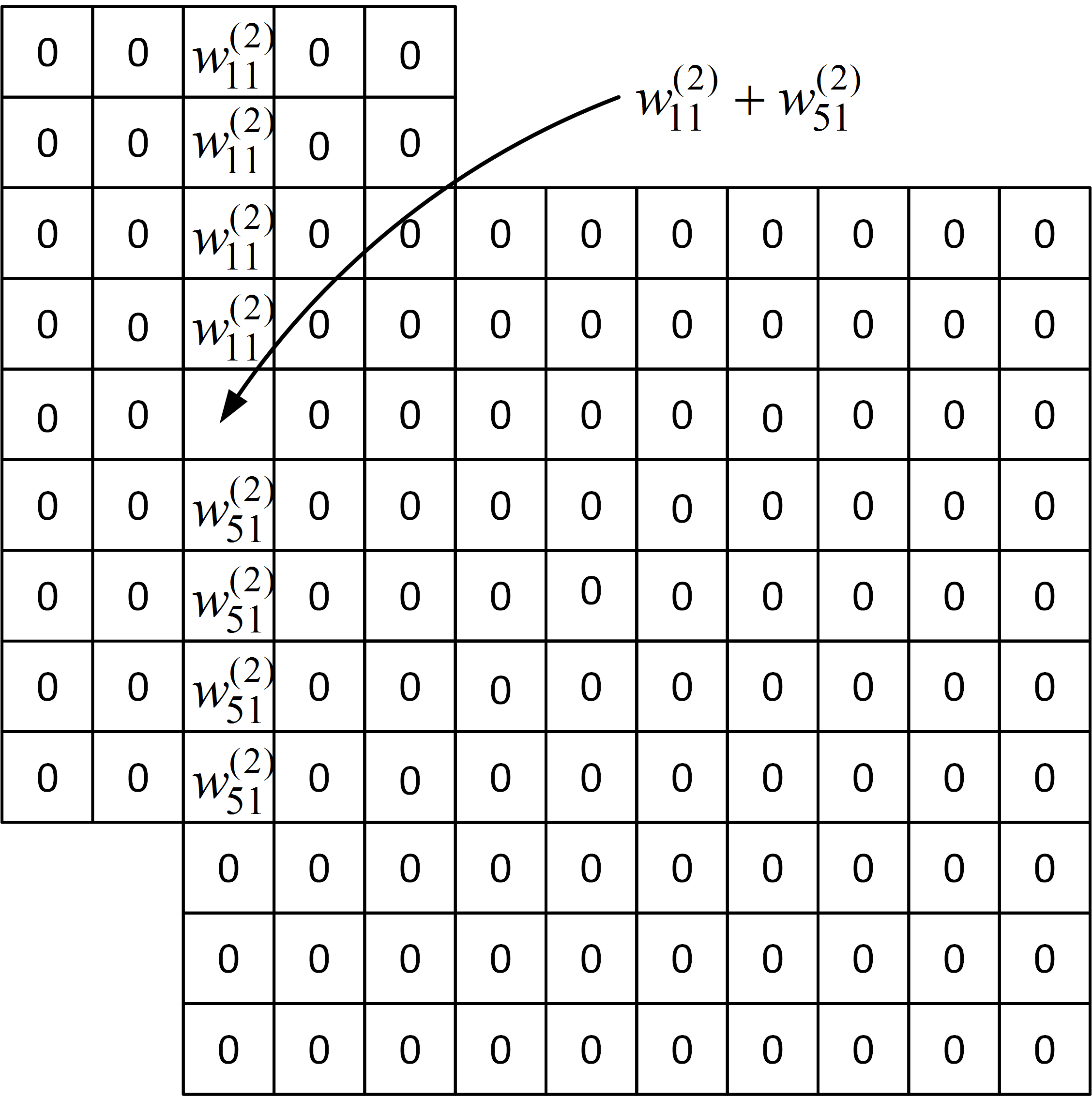
Figure 40: Reconstruction at Conv1 (L2)

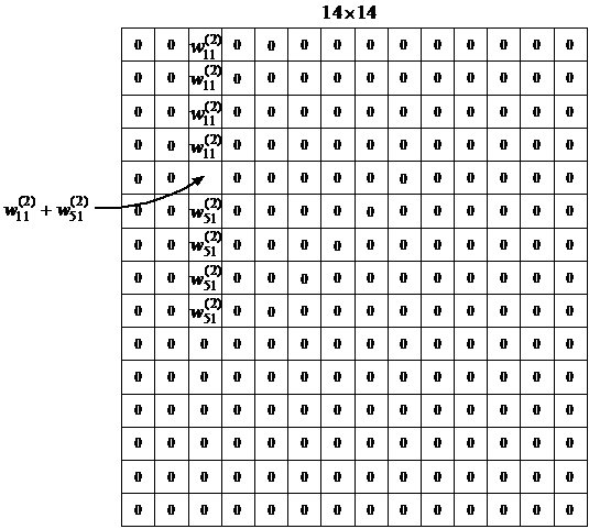
Figure 41: Reconstruction at Conv1 (L2)

Finally, 30 of these $14\times 14$ matrices are added up to make up one of the 500 features learned by neurons of L4. In other words, a particular neuron of L4 spikes when it detects its particular ($14\times 14$) feature in the original image.

Figure 42 shows 150 of the 500 reconstructed features from the 500 convolution kernels of the second convolution from L3 to L4. Each feature is $14\times 14$ neurons (pixels) of the original spiking image with ON (green) and OFF (red) features superimposed on top of each other.

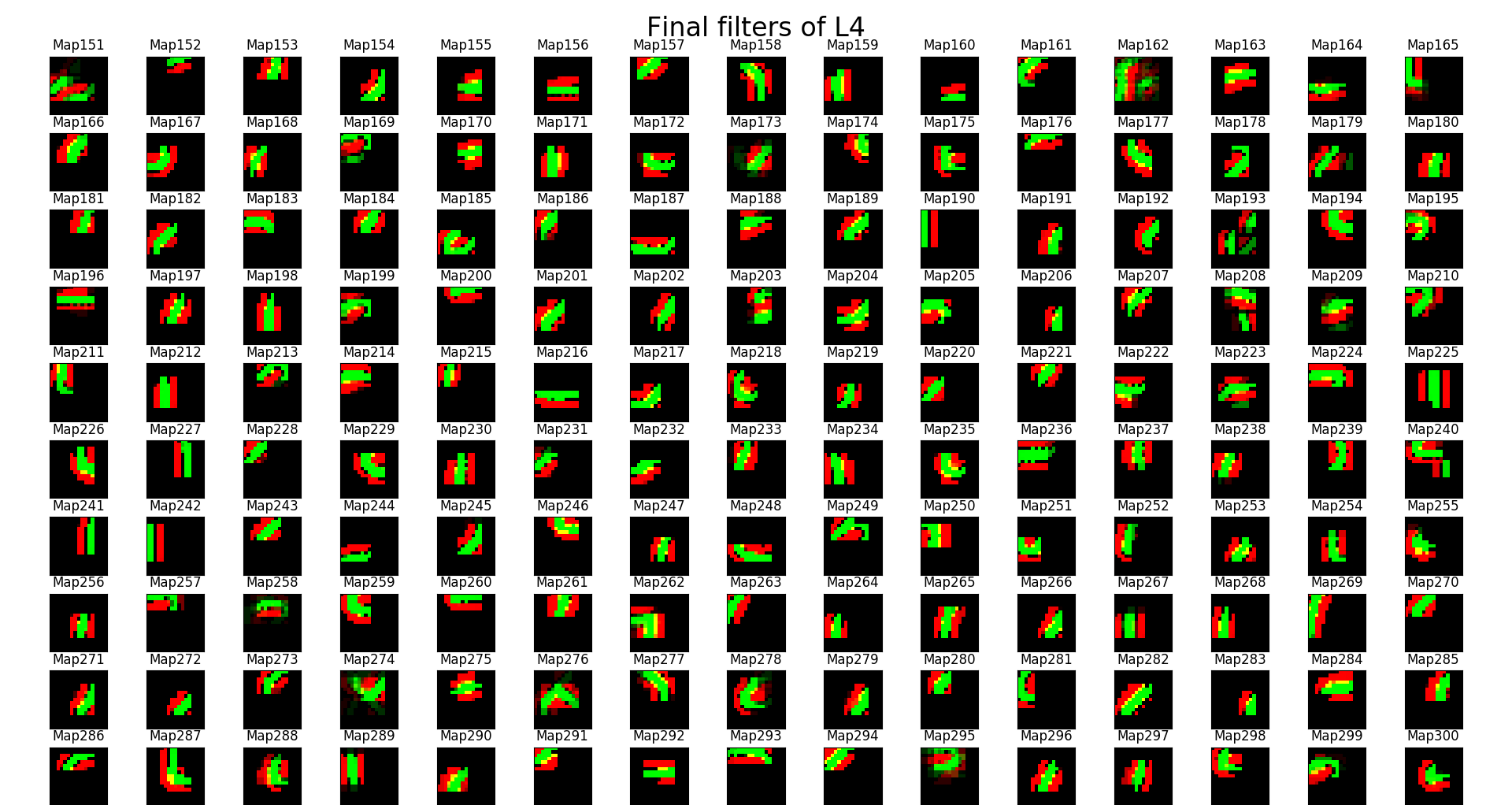
Figure 42: Weights of 150-300 maps of L4 that is trained by in coming spikes without lateral inhibition in L3, STDP competition region in L4 set to $\mathbb{R}^{500\times 3\times 3}$ and with homeostasis signal applied in L4, notice that the reconstructed features are quite complex and they could well represent a digit or a major section of a digit, note that all neurons of a map in a layer will have shared weights. In this experiment number of maps is L4 was set to 500. Notice that the reconstructed features are not as complex looking as in Figure 46

8.0.1 Effect of over training the Convolution Kernels

The first row of Figure 43 shows the reconstruction of the features from the convolution kernels of the L3 to L4 layer after training with just 20,000 images. In contrast, the second row of the Figure 43 shows the reconstruction of the features from the convolution kernels of the L3 to L4 layer after training with 60,000 MNIST images for 4 epochs. This shows that more training results in individual kernel weights ($w_{ij}$) saturating to 1 or 0 (i.e., the reconstructions in the second row are sharper), but the features become less complex.

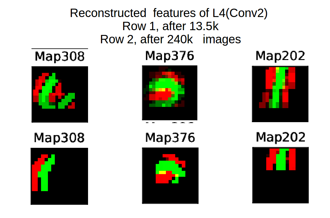
Figure 43: Reduction in the complexity of learnt features because of over training. First row of this Figure shows reconstruction of L3$\rightarrow$L4 synapses after training for 15.5k images and second row shows the reconstruction of L3$\rightarrow$L4 synapses after training for 240k images (4 epochs)

Figure 43 shows that we need a mechanism to stop training. To this end, we looked at the difference in weights during training.

$$W_{C2}^{(n)}=\{w^{(n)}(z,i,j,k)\}\in\mathbb{R}^{500\times 30\times 5\times 5}$$

where $W_{C2}^{(n)}$ is kernel $W_{C2}$ after the $n^{th}$ training is image has passed. The L3L4 (red) plot of Figure 44 is a plot of

$$\frac{\sum_{z=0}^{499}\sum_{i=0}^{29}\sum_{j=0}^{4}\sum_{k=0}^{4}\left(w^{(n\ast 150)}(z,i,j,k)-w^{((n+1)\ast 150)}(z,i,j,k)\right)}{375000}\text{ \ for \ }n=0,1,...,130$$

where $375000=500\times 30\times 5\times 5$. Similarly the L1L2 (blue) plot was done for $W_{C1}^{(n)}=\{w^{(n)}(z,i,j,k)\}\in\mathbb{R}^{30\times 2\times 5\times 5}$.

For the L3L4 the weights dramatically change between $n=80$ and $n=100.$ Multiple experiments indicated that over training of $W_{C2}$ kernels starts after $n=100$. If the network was trained further, we found that the final classification accuracy drops by by $\sim$2%.

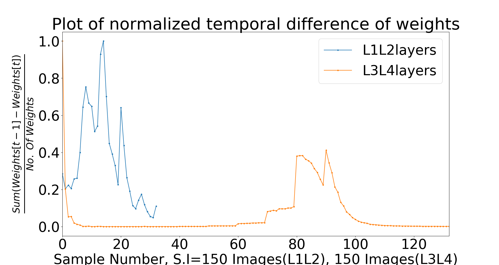
Figure 44: Plot shows the difference of successive samples of synapses, $\frac{Sum(Weights_{t}-Weights_{t-1})}{no.Of.Synapses}.$ If the difference approaches zero it means that weights are not changing hence features learnt by a neuron also remain the same. Notice the sudden jump in difference between 80-100 samples.

Kheradpisheh et al [24] proposed a convergence factor given by

$$\frac{\sum_{z=0}^{499}\sum_{i=0}^{29}\sum_{j=0}^{4}\sum_{k=0}^{4}\left(w^{(n\ast 150)}(z,i,j,k)(1\frac{{}}{{}}-w^{(n\ast 150)}(z,i,j,k))\right)}{375000}\text{ \ for \ }n=0,1,...,130.$$

The training was stopped when the convergence factor is between 0.01 and 0.02. We found that using this criteria there was a bit of over training resulting in 1%-2% decrease in testing accuracy.

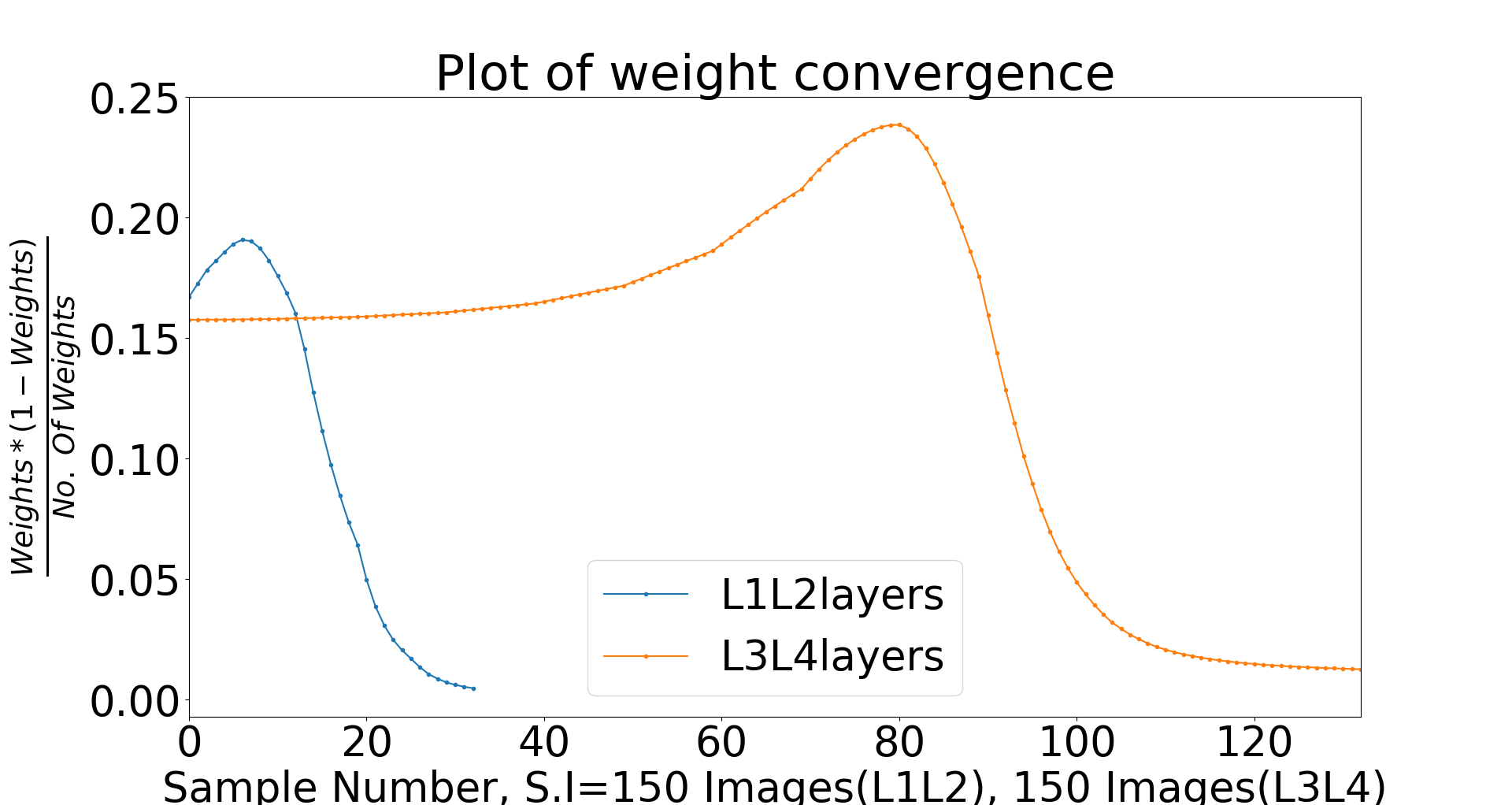
Figure 45: Plot shows the fashion of convergence for the synapses. Note that the convergence factor dips sharply between the samples 80-100.

9 Conclusion

We have studied the effects of lateral inhibition and over training in spiking convolutional networks. We reported above that using a single convolution/pool layer gives 98.4% accuracy on the MNIST data set using a two layer backprop neural network as a classifier. An accuracy of 98.8% accuracy on the MNIST data set was obtained when an SVM was used to classify the extracted features. The same experiments with the same network were carried out on the N-MNIST data set giving a 97.45% accuracy with a two layer backprop and a 98.32% accuracy using an SVM. We have demonstrated that R-STDP is sensitive to the weight initialization and a simple two layer error back propagation (avoids weight transport problem) showed better performance compared to the R-STDP classifier. We have also shown that catastrophic forgetting is not a severe problem in spiking convolutional neural networks compared to standard (non spiking) convolution networks (The spiking network still forgets, but not catastrophically!). Our spiking CNNs retained a total classification accuracy of 90.71% when trained on two disjoint sets and up to 95.1% when retrained using 10% of data from the previously trained data set.

10 Acknowledgements

We would like to express our deep gratitude to Professor Timotheé Masquelier and Dr. Saeed Reza Kheradpisheh for answering our many questions about their work [24][23]. We are also grateful to Dr. Milad Mozafari for clarifying our questions about his paper [42].

11 APPENDIX

11.1 Effect of lateral inhibition in pooling layers on subsequent convolution layers

We studied the effects of lateral inhibition [24][23] in convolution and pooling layers in terms classification accuracy and features learned. Not having lateral inhibition in pool 1 layer results in better classification provided overtrain in L4 is prevented.

11.2 With lateral inhibition in pooling layer

Features learnt in the subsequent layers tend to be more complex looking if there is lateral inhibition in this layer and less complex looking if lateral inhibition is not applied. When lateral inhibition is applied, neurons in pooling layers have no more than one spike per image thereby allowing only the most dominant neuron at a location $(u,v)$ and across all the maps to spike. So, out of all the neurons that could have spiked, the synapses of the neuron that spiked first (dominant) correlate the most with the receptive field. Hence the features that are learned in the subsequent convolution layers are more complex looking.

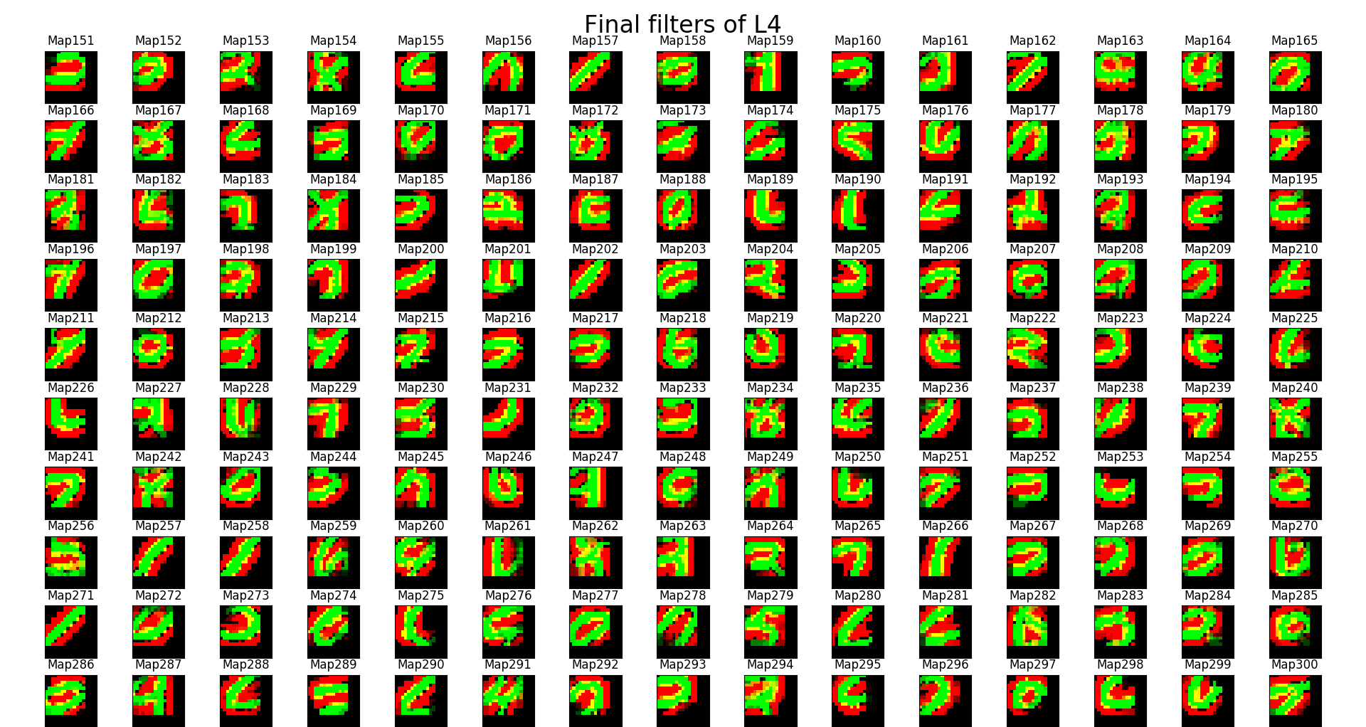
Figure 46: Weights of first 150 maps of L4 that is trained by in coming spikes with lateral inhibition in L3, STDP competition region in L4 set to $\mathbb{R}^{500\times 3\times 3}$ and with homeostasis signal applied in L4, notice that the reconstructed features are quite complex and they could well represent a digit or a major section of a digit, note that all neurons of a map in a layer will have shared weights. In this experiment number of maps is L4 was set to 500.

11.3 Scarcity of the spikes

With lateral inhibition in pooling layer (L3), number of spikes available at L4 is reduced drastically. This prevents the build up of the max pooled potentials of the L4 layer thus it gets harder for a classifier to classify these vectors.

References

- [1] J. M. Allred and K. Roy. Stimulating STDP to Exploit Locality for Lifelong Learning without Catastrophic Forgetting. arXiv e-prints, page arXiv:1902.03187, Feb 2019.
- [2] N. Anwani and B. Rajendran. Normad - normalized approximate descent based supervised learning rule for spiking neurons. In 2015 International Joint Conference on Neural Networks (IJCNN), pages 1–8, July 2015.
- [3] D. Butts, C. Weng, J. Jin, C.-I. Yeh, N. A Lesica, J.-M. Alonso, and G. Stanley. Temporal precision in the neural code and the timescales of natural vision. Nature, 449:92–5, 10 2007.
- [4] F. Chollet. Deep Learning with Python. Manning Publications Co., Greenwich, CT, USA, 1st edition, 2017.
- [5] J. Conradt, R. Berner, M. Cook, and T. Delbruck. An embedded aer dynamic vision sensor for low-latency pole balancing. In 2009 IEEE 12th International Conference on Computer Vision Workshops, ICCV Workshops, pages 780–785, Sep. 2009.
- [6] S. G. Dahl, R. Ivans, and K. D. Cantley. Modeling memristor radiation interaction events and the effect on neuromorphic learning circuits. In Proceedings of the International Conference on Neuromorphic Systems, ICONS ’18, pages 1:1–1:8, New York, NY, USA, 2018. ACM.
- [7] M. Davies, N. Srinivasa, T.-H. Lin, G. Chinya, P. Joshi, A. Lines, A. Wild, and H. Wang. Loihi: A neuromorphic manycore processor with on-chip learning. IEEE Micro, PP:1–1, 01 2018.
- [8] A. Delorme, L. Perrinet, and S. J. Thorpe. Networks of integrate-and-fire neurons using rank order coding b: Spike timing dependent plasticity and emergence of orientation selectivity. Neurocomputing, 38-40:539 – 545, 2001. Computational Neuroscience: Trends in Research 2001.
- [9] P. Diehl and M. Cook. Unsupervised learning of digit recognition using spike-timing-dependent plasticity. Frontiers in Computational Neuroscience, 9:99, 2015.
- [10] P. Ferré, F. Mamalet, and S. J. Thorpe. Unsupervised feature learning with winner-takes-all based STDP. Frontiers in Computational Neuroscience, 12:24, 2018.
- [11] R. Florian. Reinforcement learning through modulation of spike-timing-dependent synaptic plasticity. Neural computation, 19:1468–502, 07 2007.
- [12] K. Fukushima. Neocognitron: A self-organizing neural network model for a mechanism of pattern recognition unaffected by shift in position. Biological Cybernetics, 36(4):193–202, Apr 1980.
- [13] R. Girshick, J. Donahue, T. Darrell, and J. Malik. Rich feature hierarchies for accurate object detection and semantic segmentation. arXiv e-prints, page arXiv:1311.2524, Nov 2013.
- [14] T. Gollisch and M. Meister. Rapid neural coding in the retina with relative spike latencies. Science, 319(5866):1108–1111, 2008.
- [15] S. Grossberg. Competitive learning: From interactive activation to adaptive resonance. Cognitive Science, 11(1):23 – 63, 1987.
- [16] A. Gupta and L. Long. Character recognition using spiking neural networks. IEEE International Conference on Neural Networks - Conference Proceedings, pages 53 – 58, 09 2007.
- [17] D. Hassabis, D. Kumaran, C. Summerfield, and M. Botvinick. Neuroscience-inspired artificial intelligence. Neuron, 95:245–258, 07 2017.
- [18] C.-W. Hsu, C.-C. Chang, and C.-J. Lin. A practical guide to support vector classification. November 2003.
- [19] D. H. Hubel and T. N. Wiesel. Receptive fields, binocular interaction and functional architecture in the cat’s visual cortex. The Journal of Physiology, 160(1):106–154, 1962.
- [20] U. Jaramillo-Avila, H. Rostro-Gonzalez, L. A. Camuňas-Mesa, R. de Jesus Romero-Troncoso, and B. Linares-Barranco. An address event representation-based processing system for a biped robot. International Journal of Advanced Robotic Systems, 13(1):39, 2016.
- [21] Y. Jin, P. Li, and W. Zhang. Hybrid macro/micro level backpropagation for training deep spiking neural networks. arXiv-eprints, 05 2018.
- [22] S. R. Kheradpisheh. private communication.
- [23] S. R. Kheradpisheh, M. Ganjtabesh, and T. Masquelier. Bio-inspired unsupervised learning of visual features leads to robust invariant object recognition. Neurocomputing, 205:382 – 392, 2016.
- [24] S. R. Kheradpisheh, M. Ganjtabesh, S. J. Thorpe, and T. Masquelier. STDP-based spiking deep convolutional neural networks for object recognition. Neural Networks, 99:56 – 67, 2018.
- [25] M. Kiselev. Rate coding vs. temporal coding - is optimum between? In 2016 International Joint Conference on Neural Networks (IJCNN), pages 1355–1359, July 2016.
- [26] A. Krizhevsky, I. Sutskever, and G. E. Hinton. Imagenet classification with deep convolutional neural networks. Neural Information Processing Systems, 25, 01 2012.
- [27] Y. LeCun, Y. Bengio, and G. Hinton. Deep learning. Nature, 521:436–44, 05 2015.
- [28] Y. Lecun, L. Bottou, Y. Bengio, and P. Haffner. Gradient-based learning applied to document recognition. Proceedings of the IEEE, 86(11):2278–2324, Nov 1998.
- [29] Y. LeCun and C. Cortes. MNIST handwritten digit database. 2010.
- [30] C. Lee, P. Panda, G. Srinivasan, and K. Roy. Training deep spiking convolutional neural networks with STDP-based unsupervised pre-training followed by supervised fine-tuning. Frontiers in Neuroscience, 12:435, 08 2018.
- [31] J. H. Lee, T. Delbruck, and M. Pfeiffer. Training deep spiking neural networks using backpropagation. Frontiers in Neuroscience, 10:508, 2016.
- [32] R. Legenstein, D. Pecevski, and W. Maass. Theoretical analysis of learning with reward-modulated spike-timing-dependent plasticity. arXiv e-prints, 20, 01 2007.
- [33] Q. Liao, J. Z. Leibo, and T. Poggio. How Important is Weight Symmetry in Backpropagation? arXiv e-prints, page arXiv:1510.05067, Oct 2015.
- [34] T. Lillicrap, D. Cownden, D. Tweed, and C. J. Akerman. Random synaptic feedback weights support error backpropagation for deep learning. Nature Communications, 7:13276, 11 2016.
- [35] Q. Liu, G. Pineda-Garcĩa, E. Stromatias, T. Serrano-Gotarredona, and S. B. Furber. Benchmarking spike-based visual recognition: A dataset and evaluation. Frontiers in Neuroscience, 10:496, 2016.
- [36] H. Markram, W. Gerstner, and P. J. Sjöström. Spike-timing-dependent plasticity: A comprehensive overview. Frontiers in Synaptic Neuroscience, 4:2, 2012.
- [37] T. Masquelier. Spike-based computing and learning in brains, machines, and visual systems in particular (HDR Report). PhD thesis, 10 2017.
- [38] T. Masquelier, R. Guyonneau, and S. J. Thorpe. Spike timing dependent plasticity finds the start of repeating patterns in continuous spike trains. PLOS ONE, 3(1):1–9, 01 2008.
- [39] T. Masquelier and S. J. Thorpe. Unsupervised learning of visual features through spike timing dependent plasticity. PLoS Computational Biology, 3:1762 – 1776, 2007.
- [40] B. Meftah, O. Lezoray, and A. Benyettou. Segmentation and edge detection based on spiking neural network model. Neural Processing Letters, 32(2):131–146, Oct 2010.
- [41] M. Mozafari, M. Ganjtabesh, A. Nowzari, S. Thorpe, and T. Masquelier. Combining STDP and reward-modulated STDP in deep convolutional spiking neural networks for digit recognition. arXiv e-prints, 03 2018.
- [42] M. Mozafari, S. R. Kheradpisheh, T. Masquelier, A. Nowzari-Dalini, and M. Ganjtabesh. First-spike-based visual categorization using reward-modulated STDP. IEEE Transactions on Neural Networks and Learning Systems, 29(12):6178–6190, Dec 2018.
- [43] E. O. Neftci, C. Augustine, S. Paul, and G. Detorakis. Event-driven random back-propagation: Enabling neuromorphic deep learning machines. Frontiers in Neuroscience, 11:324, 2017.
- [44] B. Nessler, M. Pfeiffer, L. Buesing, and W. Maass. Bayesian computation emerges in generic cortical microcircuits through spike-timing-dependent plasticity. PLOS Computational Biology, 9(4):1–30, 04 2013.
- [45] M. A. Nielsen. Neural Networks and Deep Learning, Jan 2015.
- [46] G. Orchard, A. Jayawant, G. K. Cohen, and N. Thakor. Converting static image datasets to spiking neuromorphic datasets using saccades. Frontiers in Neuroscience, 9:437, 2015.
- [47] L. Paulun, A. Wendt, and N. Kasabov. A retinotopic spiking neural network system for accurate recognition of moving objects using neucube and dynamic vision sensors. Frontiers in Computational Neuroscience, 12:42, 2018.
- [48] M. Pfeiffer and T. Pfeil. Deep learning with spiking neurons: Opportunities and challenges. Frontiers in Neuroscience, 12:774, 2018.
- [49] C. Posch, D. Matolin, R. Wohlgenannt, M. Hofstätter, P. Schön, M. Litzenberger, D. Bauer, and H. Garn. Live demonstration: Asynchronous time-based image sensor (atis) camera with full-custom ae processor. In Proceedings of 2010 IEEE International Symposium on Circuits and Systems, pages 1392–1392, May 2010.
- [50] P. Reinagel and R. C. Reid. Temporal coding of visual information in the thalamus. Journal of Neuroscience, 20(14):5392–5400, 2000.
- [51] A. Rocke. The weight transport problem, Jun 2017.
- [52] B. Rueckauer, I.-A. Lungu, Y. Hu, and M. Pfeiffer. Theory and Tools for the Conversion of Analog to Spiking Convolutional Neural Networks. arXiv e-prints, page arXiv:1612.04052, Dec 2016.
- [53] V. Saxena, X. Wu, I. Srivastava, and K. Zhu. Towards neuromorphic learning machines using emerging memory devices with brain-like energy efficiency. Journal of Low Power Electronics and Applications, 8(4), 2018.
- [54] J. Schmidhuber. Deep learning in neural networks: An overview. Neural Networks, 61:85 – 117, 2015.
- [55] E. Shelhamer, J. Long, and T. Darrell. Fully convolutional networks for semantic segmentation. IEEE Transactions on Pattern Analysis and Machine Intelligence, 39(4):640–651, April 2017.
- [56] J. Sjöström and W. Gerstner. Spike-Timing Dependent Plasticity. Scholarpedia, 5(2):1362, 2010. revision #184913.
- [57] S. Skorheim, P. Lonjers, and M. Bazhenov. A spiking network model of decision making employing rewarded STDP. PLOS ONE, 9(3):1–15, 03 2014.
- [58] E. Stromatias, M. Soto, T. Serrano-Gotarredona, and B. L.-B. Linares-Barranco. An event-driven classifier for spiking neural networks fed with synthetic or dynamic vision sensor data. Frontiers in Neuroscience, 11:350, 2017.
- [59] A. Tavanaei, M. Ghodrati, S. R. Kheradpisheh, T. Masquelier, and A. S. Maida. Deep Learning in Spiking Neural Networks. arXiv e-prints, page arXiv:1804.08150, Apr 2018.
- [60] A. Tavanaei, Z. Kirby, and A. Maida. Training spiking convnets by STDP and gradient descent. 2018 International Joint Conference on Neural Networks (IJCNN), pages 1–8, 07 2018.
- [61] A. Tavanaei and A. S. Maida. Multi-layer unsupervised learning in a spiking convolutional neural network. In 2017 International Joint Conference on Neural Networks (IJCNN), pages 2023–2030, May 2017.
- [62] A. Tavanaei, T. Masquelier, and A. S. Maida. Acquisition of visual features through probabilistic spike-timing-dependent plasticity. 2016 International Joint Conference on Neural Networks (IJCNN), pages 307–314, July 2016.
- [63] R. VanRullen. Perception science in the age of deep neural networks. Frontiers in Psychology, 8:142, 2017.
- [64] X. Wu and V. Saxena. Dendritic-inspired processing enables bio-plausible stdp in compound binary synapses. IEEE Transactions on Nanotechnology, PP, 01 2018.
- [65] X. Wu, V. Saxena, and K. Zhu. Homogeneous spiking neuromorphic system for real-world pattern recognition. IEEE Journal on Emerging and Selected Topics in Circuits and Systems, 5(2):254–266, June 2015.
- [66] X. Wu, V. Saxena, K. Zhu, and S. Balagopal. A cmos spiking neuron for brain-inspired neural networks with resistive synapses andin situlearning. IEEE Transactions on Circuits and Systems II: Express Briefs, 62(11):1088–1092, Nov 2015.
- [67] D. Zambrano, R. Nusselder, H. S. Scholte, and S. M. Bohté. Sparse computation in adaptive spiking neural networks. Frontiers in Neuroscience, 12:987, 2019.
- [68] J. Zylberberg, J. T. Murphy, and M. R. Deweese. A sparse coding model with synaptically local plasticity and spiking neurons can account for the diverse shapes of v1 simple cell receptive fields, 2011.