Efficient approximation of flow problems with multiple scales in time

Abstract

In this article we address flow problems that carry a multiscale character in time. In particular we consider the Navier-Stokes flow in a channel on a fast scale that influences the movement of the boundary which undergoes a deformation on a slow scale in time. We derive an averaging scheme that is of first order with respect to the ratio of time-scales $\epsilon$. In order to cope with the problem of unknown initial data for the fast scale problem, we assume near-periodicity in time. Moreover, we construct a second-order accurate time discretisation scheme and derive a complete error analysis for a corresponding simplified ODE system. The resulting multiscale scheme does not ask for the continuous simulation of the fast scale variable and shows powerful speed-ups up to 1:10 000 compared to a resolved simulation. Finally, we present some numerical examples for the full Navier-Stokes system to illustrate the convergence and performance of the approach.

1 Introduction

We are interested in the numerical approximation and long-term simulation of flow problems that carry a multiscale character in time. Such problems appear for example in the formation of atherosclerotic plaque in arteries, where flow dynamics acting on a scale of milliseconds to seconds have an effect on plaque growth in the vessel, which typically takes place within a range of several months. Another application is the investigation of chemical flows in pipelines, where long-time effects of weathering, accelerated by the transported substances, cause material alteration.

These examples have in common, that it is computationally infeasible to resolve the fast scale over the whole time interval of interest. In the case of atherosclerotic plaque growth, a suitable time-step of $\frac{1}{20}\,\mathrm{s}$ would require nearly $10^{9}$ steps to cover the period of interest, which is at least $6\,\mathrm{months}$.

Inspired by the temporal dynamics of atherosclerotic plaque growth, we will consider the flow in a channel whose boundary is deformed over a long time scale. This deformation is controlled by the concentration variable $u(t)$ that is governed by a simple reaction equation and that depends on the fluid-forces

$$\mathbf{v}(0) =\mathbf{v}_{0}, \quad\operatorname{div}\,\mathbf{v} =0,\quad\rho(\partial_{t}\mathbf{v}+(\mathbf{v}\cdot\nabla)\mathbf{v})-{\operatorname{div}}\,\boldsymbol{\sigma}(\mathbf{v},p)=\mathbf{f} \Omega(u(t))$$     in (1)

$$u(0) =0, \quad u^{\prime} =\epsilon R(u,\mathbf{v}).$$

Here, $\rho$ is the density of the fluid, $\boldsymbol{\sigma}=\rho\nu(\nabla\mathbf{v}+\nabla\mathbf{v}^{T})-pI$ the Cauchy stress with the kinematic viscosity $\nu$ and $R(\mathbf{v},u)\geq 0$ a reaction term describing the influence of the fluid forces (namely the wall shear stress) on the boundary growth. The growth term $R(\cdot,\cdot)$ it modeled such that $|R(\cdot,\cdot)|={\cal O}(1)$:

$$R(u,\mathbf{v})\coloneqq\big{(}1+u\big{)}^{-1}\big{(}1+|\sigma_{WSS}(\mathbf{v})|^{2}\big{)}^{-1},\quad\sigma_{WSS}(\mathbf{v})\coloneqq\sigma_{0}^{-1}\int_{\Gamma}\rho\nu\big{(}I_{d}-\vec{n}\vec{n}^{T}\big{)}(\nabla\mathbf{v}+\nabla\mathbf{v}^{T})\vec{n}\,\text{d}o,$$ (2)

where $\vec{n}$ denotes the outward facing unit normal vector at the boundary $\Gamma$. The parameter $\sigma_{0}>0$ will be tuned to give $|\sigma_{WSS}(v)|={\cal O}(1)$, see Section 5. The domain $\Omega=\Omega(u(t))$ depends explicitly on the concentration $u(t)$. We show a sketch of the configuration in Figure 1. The flow problem is driven by a periodic oscillating inflow profile of period $1\,\mathrm{s}$

$$\mathbf{v}=\mathbf{v}^{D}\text{ on }\Gamma_{in},\text{ with }\mathbf{v}^{D}(t)=\mathbf{v}^{D}(t+1s).$$

This period describes the fast scale of the problem. By $\epsilon\ll 1$ we denote a small parameter that controls the time scale of the (slow) growth of the concentration, i.e. $|u^{\prime}|={\cal O}(\epsilon)$ and $T={\cal O}(\epsilon^{-1})$ is the expected long term horizon. While the problem itself is strongly simplified compared to the detailed non-linear mechano-chemical FSI model of plaque-growth [8, 50, 17], we choose the parameters in such a way that the temporal dynamics are very similar.

The structure of this article is as follows: In Section 2 we introduce a simple model problem consisting of two coupled ODEs, that are related to (1), and for which we will be able to conduct a complete error analysis. Moreover, we discuss some of the available approaches in literature and outline the multiscale algorithm developed in this article. In Section 3 we derive the effective long term equations and give an error analysis on the continuous level. In Section 4 we describe the temporal discretisation of the multiscale scheme and show optimal order convergence in all discretisation parameters: mesh size $h$, time step size $k$ for the fast problem and time step size $K$ for the slowly evolving variable. In Section 5 we apply the multiscale scheme to the complex problem introduced in Section 2, which is based on the Navier-Stokes equations. We show numerically optimal-order convergence in agreement to the theoretical findings for the simplified system. We conclude with a short summary and a discussion of some open problems.

Figure 1: Configuration of the test case. We study flow in a channel with a boundary $\Gamma$ that depends on a concentration variable $u$. This $u$ follows a simple reaction law with a right-hand side depending on the wall shear stress on $\Gamma_{wall}$.

2 Time scales

In this section we start by analyzing the temporal multiscale character of the plaque formation problem. We simplify the coupled problem and introduce a model problem coupling two ODEs. Then, we present various approaches for the numerical treatment of temporal multiscale problems that are discussed in literature. Finally we sketch the idea of the multiscale scheme that is considered in this work, which fits into the framework of the heterogeneous multiscale method.

2.1 A model problem

To start with, we introduce a simple model problem, a system of two ODEs that shows the same coupling and temporal multiscale characteristics as the full plaque growth system

$$u(0) =u_{0}, \quad u^{\prime}(t) =\epsilon R(u(t),v(t))$$ (3a)

$$v(0) =v_{0}, \quad v^{\prime}(t)+\lambda(u(t))v(t) =f(t),$$ (3b)

where $f(t)=f(t+1)$ is periodic and $R(\cdot,\cdot)$ is given by

$$R(u,v)\coloneqq\big{(}1+u\big{)}^{-1}\big{(}1+v^{2}\big{)}^{-1}.$$ (4)

For the reaction term it holds $|R(u,v)|\leq 1$. The parameter $\lambda(u)\geq\lambda_{0}>0$ depends on the concentration $u$. We will assume that the relation $u\to\lambda(u)$ is differentiable and that the derivative $\frac{d\lambda(u)}{du}$ remains bounded.

In Section 5.2 we will argue that this system can indeed be considered as a simplification of the full plaque growth system by neglecting the nonlinearity and by diagonalizing the resulting Stokes equation with respect to an orthonormal eigenfunction basis. Moreover, if we introduce $\tau\coloneqq\epsilon t$, $v_{\tau}(\tau)\coloneqq v(t)$, $u_{\tau}(\tau)\coloneqq u(t)$ as well as $f_{\tau}(\tau)\coloneqq f(t)$ we can scale this system to

$$v_{\tau}(0)=v_{0},\;u_{\tau}(0)=u_{0},\quad v_{\tau}^{\prime}+\epsilon^{-1}\lambda(u_{\tau})v_{\tau}=\epsilon^{-1}f_{\tau},\;u_{\tau}^{\prime}=R(u_{\tau},v_{\tau}),$$ (5)

which reveals the typical character of ODE systems with multiple scales in time as discussed in [14, 1]. In the language of the heterogeneous multiscale method (HMM), see also [15], such a problem is called a type B problem and it is characterized by the acting of fast and slow scales throughout the whole (long) time span $[0,T]$ in contrast to problems with localised singular behavior. Since $|R|={\cal O}(1)$ it holds $|u^{\prime}_{\tau}|={\cal O}(1)$ and $u_{\tau}$ describes the slow variable while $|v^{\prime}_{\tau}|={\cal O}(\epsilon^{-1})$ indicates the fast and oscillatory variable.

2.2 Numerical approaches for temporal multiscale problems

While multiscale problems in space are extensively studied in literature, see e.g. [10, 38], less works are found on problems with multiscale character in time. Some literature exists that uses a homogenisation approach based on asymptotic expansions in time for viscoelastic, viscoplastic or elasto-viscoplastic solids [22, 52, 3, 24]. Under suitable assumptions, the short-scale part of the multiscale algorithm becomes stationary for this class of equations, such that difficulties to define initial values on the short scale are avoided.

Multirate time stepping methods [20] split the system into slow and large components and use different time step sizes according to the dominant scales. All scales are still resolved on the complete time interval. Since the fast scale of problems (1) which requires a small time step is the computationally intensive Navier-Stokes equations and since the scales are vastly separated, such multirate methods are not appropriate for the problem under investigation.

In the context of continuum damage mechanics, processes with high frequent oscillatory impact can be approached by block cycle jumping techniques [33], where a large number of cycles is skipped and replaced by linear approximation of the damage effect. An overview of different techniques is given in the first two introductionary sections of [7]. These approaches do not resolve the complete system on full temporal interval but reside on local solutions. This gives rise to the problem of finding initial values.

If the time scales are close enough that the short-scale dynamics can be resolved within one time step of the long-scale discretisation, the Variational Multiscale Method [28, 6] or approaches that construct long-scale basis functions from the short-scale information [39, 2] are applicable. Similar algorithms are also used to construct parallel-in time integrators, for example the parareal method [35]. In this work, we are interested in problems with a stronger scale separation, where the resolution of the short scale within a long-scale interval is very costly up to computationally unfeasible.

Only very few numerical works can be found concerning flow problems with multiple scales in time. An exception are the works of Masud & Khurram [36, 31], where the Variational Multiscale Method is applied, assuming again that the time scales are sufficiently close. On the other hand, several theoretical works exist that show convergence towards averaged equations for specific flow configurations in the situation that the ratio of time scales $\epsilon=\frac{t_{\text{fast}}}{T_{\text{long}}}$ tends to zero, see e.g. [29, 9, 34], however without considering practical numerical algorithms or discretisation.

A common numerical approach is to replace the fast problem by an averaged one using a fixed-in-time inflow profile [50, 8]. It is however widely accepted and also confirmed in numerical studies [17] that such a simple averaging does not necessarily reproduce the correct dynamics. In [17] we presented a first multiscale scheme for the approximation of such a problem, however with a focus on the modelling of a full closure of the channel and without any analysis on the robustness and accuracy. Similar algorithms can be found in Sanders et al [44] and by Crouch & Oskay [11] in different applications. In this work, we will derive an improved algorithm in a mathematically rigorous way, including a detailed error analysis for both modelling and discretisation errors. To our knowledge this is the first time that the interplay between modelling errors of the temporal multiscale scheme and temporal discretisation errors on both scales is analysed.

One of the most prominent class of techniques is the heterogeneous multiscale method (HMM) [15, 14, 1, 16] that aims at an efficient decoupling of macro-scale and micro-scale, where the latter one enters the macro-scale problem in terms of temporal averages. Typically, the procedure is as follows: one determines the fast and the slow variables of the coupled problem. For the slow variables an integrator with a long time step $\Delta T\coloneqq T_{n+1}-T_{n}$ and good stability properties is used. At each of these macro time steps, the fast scale problem is initialized based on the current slow variable and solved on the interval $I_{n}^{\eta}\coloneqq[T_{n},T_{n}+\eta]$. Finally, the fast variable output on $I_{n}^{\eta}$ is averaged to yield the effective operator for the slow scale problem.

The efficiency of the resulting HMM scheme depends on the choice of $\eta$ which indicates the scale to allow for equilibration and adjustment of the micro model. Too large values will reduce the efficiency, too small values will limit the accuracy. The underlying problem is the lack of initial values at the new macro step for the fast scale, which in our case (1) or (3), is the oscillatory velocity $\mathbf{v}(t)$ and $v(t)$, respectively. The realisation presented in this article is based on time-periodic solutions to the micro problem. Instead of solving the microscale problem on an interval $I_{n}^{\eta}$ at macro step $T_{n}$ we aim at a localised solution of the fluid problem that satisfies a periodicity condition in time. This approach allows us to conduct a complete error analysis of the resulting scheme when applied to the simplified model problem (3).

2.3 Outline of the multiscale scheme

We conclude this section by briefly describing the multiscale algorithm that is considered in this article. The derivation given here is based on problem (3). We start by defining the slow variable as average of the concentration $u(t)$

$$U(t)\coloneqq\int_{t}^{t+1\,\mathrm{s}}u(s)\,\text{d}s.$$ (6)

This gives rise to the averaged equation for the long term dynamics

$$U^{\prime}(t)=\int_{t}^{t+1}\epsilon R(u(s),v(s))\,\text{d}s$$ (7)

A time integration formula with a macro time-step is used to approximate this equation. Two approximation steps are performed to reach an effective equation. First, the reaction term in (7) is evaluated in $U(t)$ instead of $u(s)$ and second, the fast component $v(s)$ will be replaced by the localised solution of the time-periodic problem obtained for a fixed value of $U(t)$:

$$v^{\prime}_{U(t)}+\lambda(U(t))v_{U(t)}=f\text{ in }[0,1]\text{ with }v_{U(t)}(1)=v_{U(t)}(0).$$ (8)

These approximations will be discussed and analysed in the following section. Assuming that (7), approximated in these two steps, is integrated with the forward Euler method, a macro time step is given by

$$U_{n}=U_{n-1}+(T_{n}-T_{n-1})\int_{T_{n-1}}^{T_{n}}\epsilon R(U_{n-1},v_{U_{n-1}}(s))\,\text{d}s.$$ (9)

2.3.1 Motivation for the locally periodic approximations

Due to the nonlinearity of the reaction term $R(\cdot,\cdot)$, the micro-scale variations in $v(s)$ can not simply be averaged. Instead the velocities $v(s)$ need to be computed on the fast scale in each macro step $T_{n-1}\to T_{n}$, in order to obtain a good approximation of the integral on the right-hand side of (7). A computation of $v(s)$ over the complete interval $[T_{n-1},T_{n}]$ is however unfeasible for small $\epsilon$. For this reason, the imposition of accurate initial values $v(T_{n})$ for the fast-scale problem is not straight-forward. Neither the short-scale velocity $v(T_{n-1})$ from the previous macro-time step nor an averaged quantity $V(T_{n})$ can guarantee a sufficiently good approximation for $v(T_{n})$. In practice, a relaxation time $\eta$ is frequently introduced (see for example [16, 1]), in order to improve the initial values by means of a few forward iterations.

As an alternative, we propose to introduce the time-periodic fast-scale problem (8). This has the advantage that in principle only one period of the fast-scale problem needs to be resolved per macro-step. We can show theoretically (Lemma 8) that the approximation error introduced by the periodic problem is of order $\epsilon$. Efficient approximations of these time-periodic problems will be discussed in Section 4.3.

2.3.2 Abstract multiscale scheme

We conclude this section by formulating the abstract multiscale scheme that can be applied to both problems, the plaque growth system and the simplified model problem. [Abstract Multiscale Scheme] Let $0=T_{0}<T_{1}<\dots<T_{N}=T$ be a partition of the macro interval with uniform step size $K\coloneqq T_{n}-T_{n-1}$. Further, let $U_{0}\coloneqq u_{0}$ be the initial value of the slow variable. Iterate for $n=1,2,\dots$

1. Solve the time-periodic problem (12) or (13) for $\mathbf{v}_{U_{n-1}}$.

2. Evaluate the reaction term

   $$R_{n-1}\coloneqq\int_{0}^{1}R(U_{n-1},\mathbf{v}_{U_{n-1}}(s))\,\text{d}s$$

3. Forward the slow variable with an (explicit) one-step scheme

   $$U_{n}={\cal F}(K;U_{n-1};R_{n-1})$$

The structure of the time integrator ${\cal F}$ depends on the system of equations and the time-stepping method. For simplicity, we have formulated the algorithm for an explicit time integrator in the slow variable. The use of an implicit time stepping scheme would require an iterated evaluation of the periodic problem for updated values of $U_{n}$. In the case of $r$-step schemes periodic solutions $\mathbf{v}_{U_{n-k}}$ would be required for $k=1,\dots,r$.

Remark 2.1.

We note that the proposed algorithm does not compute an average of the fast variable $v$. An approximation to $v$ is only computed on the short periodic interval of the fast-scale as $\mathbf{v}_{U_{n-1}}$ (Step 1). The slow variable $u$, on the other hand, is only computed on the slow scale as average $U$ (Step 3).

The typical behaviour of the slow and fast variables is illustrated in Figure 2 (top). On the bottom of Figure 2, the multiscale algorithm is visualised, including the transfer of quantities between the slow and the fast scale. For ease of presentation a large $\epsilon$ has been chosen for the purpose of visualisation.

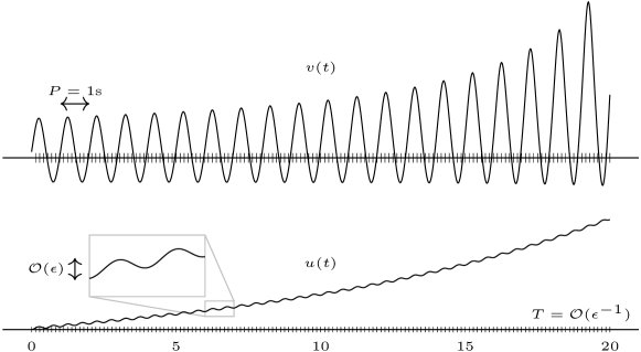
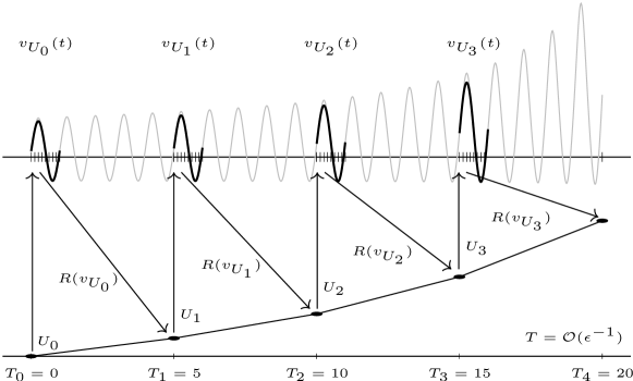
Layout of the multiscale problem. The fast variable $v(t)$ (top) and the “slow” variable $u(t)$ (bottom) couple on the complete long time interval $I=[0,T]$. The “slow” variable is also oscillating, but the oscillations are small, of size ${\cal O}(\epsilon)$. The fast variable is locally nearly periodic.

Figure 2: Construction of the multiscale scheme: 0. The slow variable $U(t)$ is discretised with a time-stepping scheme with macro step size $K\gg 1$. 1. In each step the current slow state $U_{n-1}$ is transferred to the fast problem (top) and a periodic solution $\mathbf{v}_{U_{n-1}}$ is computed on $[T_{n-1},T_{n-1}+1]$ as approximation for $\mathbf{v}(t)$. 2. The averaged reaction term $R_{n-1}=R(\mathbf{v}_{U_{n-1}})$ is computed from $\mathbf{v}_{U_{n-1}}$ and transferred to the slow problem (bottom). 3. The slow variable $U_{n}$ is updated by the macro step $T_{n-1}\to T_{n}$.

To conclude this section we anticipate the main result of the analysis given below. For the combination of the second order Adams-Bashforth rule for the discretisation of the slow problem and the Crank-Nicolson scheme for the fast problem we will show optimal convergence of the resulting multiscale scheme:

$$|U_{N}-u(T)|={\cal O}(\epsilon)+{\cal O}(\epsilon^{2}K^{2})+{\cal O}(k^{2})+{\cal O}(\text{tol}_{P}).$$

By $K$ we denote the step size of the macro solver, $k$ is the step size of the micro solver and by $\text{tol}_{P}$ we denote the tolerance of the periodicity constraint: $\max_{n}|v_{U_{n}}(1)-v_{U_{n}}(0)|<\text{tol}_{P}$.

3 Derivation and analysis of the effective equations

In this section we derive the temporal multiscale scheme that has been outlined in the previous section. We will discuss the coupled Navier-Stokes problem on the evolving domain $\Omega(u)$, problem (1) and the reduced ODE system (3) side by side. Whenever results apply to the ODE system only, we will clearly mention this. We start by collecting some preliminary assumptions on the underlying problems.

3.1 Preliminaries

[Reaction term] Let $u_{max}<\infty$ be a maximum concentration. Let $0\leq u\leq u_{max}$ and $\mathbf{v}\in X$ ($X=\mathds{R}$ for the model problem, $X=H^{2}(\Omega)$ for the plaque growth problem). The reaction term is bounded

$$|R(u,\mathbf{v})|\leq C_{A\ref{ass:reaction}a},$$ (10)

and Lipschitz continuous in both arguments

$$|R(u_{1},\mathbf{v})-R(u_{2},\mathbf{v})|\leq C_{A\ref{ass:reaction}b}|u_{1}-u_{2}|,\quad|R(u,\mathbf{v}_{1})-R(u,\mathbf{v}_{2})|\leq C_{A\ref{ass:reaction}b}\|\mathbf{v}_{1}-\mathbf{v}_{2}\|_{X},$$ (11)

where the constant $C$ does not depend on $\epsilon$.

Assumption 3.1 is easily verified for the simplified reaction term (4). A proof for Navier-Stokes case will be given in Section 5.2.

Remark 3.1 (Generic constants).

Throughout this manuscript we use generic constants $C$. These constants may depend on the domain $\Omega$, the maximum concentration $u_{max}$, the right hand side $\mathbf{f}$ and the Dirichlet data. They do, however, not depend on the solution, the scale parameter $\epsilon$ or the discretisation parameters that will be introduced in the remainder of this article.

We further assume that the isolated micro problems allow for a unique periodic solution: [Periodic solution] Let $u\in\mathds{R}$ with $0\leq u\leq u_{max}$. We assume that there exist unique periodic solutions $v_{u}\in C([0,1])$ to

$$\partial_{t}v_{u}+\lambda(u)v_{u}=f\text{ in }[0,1],\quad v_{u}(1)=v_{u}(0),$$ (12)

as well as solutions $\mathbf{v}_{u}\in H^{2}(\Omega(u),p_{u}\in H^{1}(\Omega(u))$ to the incompressible Navier-Stokes equations

$$\nabla\cdot\mathbf{v}_{u}=0,\quad\rho(\partial_{t}\mathbf{v}_{u}+(\mathbf{v}_{u}\cdot\nabla)\mathbf{v}_{u})-{\operatorname{div}}\,\boldsymbol{\sigma}(\mathbf{v}_{u},p_{u}) =\mathbf{f} \text{in }[0,1]\times\Omega(u)$$ (13a)

$$\mathbf{v}_{u} =\mathbf{v}^{D}_{u} \text{on }[0,1]\times\partial\Omega(u)$$ (13b)

$$\mathbf{v}_{u}(1) =\mathbf{v}_{u}(0) \text{in }\Omega(u)$$ (13c)

Both solutions are uniformly bounded in time

$$\sup_{t\in[0,T]}|v_{u}(t)|\leq C,\quad\sup_{t\in[0,T]}\Big{(}\|\mathbf{v}_{u}(t)\|_{H^{2}(\Omega)}+\|p_{u}(t)\|_{H^{1}(\Omega)}\Big{)}\leq C.$$ (14)

For the ODE problem (12), the existence of a unique periodic solutions follows from the evolution of $w(t)=v(t+1)-v(t)$ which fulfills $w^{\prime}+\lambda(u)w=0$ and thus vanishes, see [42]. For a discussion on the Navier-Stokes equations we refer to Section 5.2.

3.2 Derivation of an effective equation

We introduce the averaged concentration

$$U(t)\coloneqq\int_{t}^{t+1}u(s)\,\text{d}s.$$

Using (1) and (3), respectively, and inserting $\pm R\big{(}U(t),\mathbf{v}(s)\big{)}$, we have

$$U^{\prime}(t)=\int_{t}^{t+1}\epsilon R\big{(}u(s),\mathbf{v}(s)\big{)}\,\text{d}s=\int_{t}^{t+1}\epsilon R\big{(}U(t),\mathbf{v}(s)\big{)}\,\text{d}s-\int_{t}^{t+1}\epsilon\left(R\big{(}U(t),\mathbf{v}(s)\big{)}-R\big{(}u(s),\mathbf{v}(s)\big{)}\right)\,\text{d}s.$$

Lemma 3.2 (Averaging error).

Let $u\in C^{1}([0,T])$, $\mathbf{v}\in C([0,T];X)$ and let Assumption 3.1 be satisfied. Then, it holds

$$\max_{t}\Big{|}\int_{t}^{t+1}\left(R(U(t),\mathbf{v}(s))-R(u(s),\mathbf{v}(s))\right)\,\text{d}s\Big{|}\leq C\epsilon,$$

with a constant $C>0$ that depends on Assumption 3.1.

Proof 3.3.

By Lipschitz continuity of $R(\cdot,\cdot)$ in the first argument (11) it holds

$$|R(U(t),\mathbf{v}(s))-R(u(s),\mathbf{v}(s))|\leq C|u(s)-U(t)|.$$ (15)

We estimate

$$\int_{t}^{t+1}|u(s)-U(t)|\,\text{d}s=\int_{t}^{t+1}\left|\int_{t}^{t+1}(u(s)-u(r))\,\text{d}r\right|\,\text{d}s=\int_{t}^{t+1}\left|\int_{t}^{t+1}\int_{r}^{s}u^{\prime}(x)\,\text{d}x\,\text{d}r\right|\,\text{d}s\leq C\epsilon,$$ (16)

where we used (10), such that a combination of (15) and (16) shows the assertion.

We can thus approximate the averaged evolution equation for $U$ by

$$U^{\prime}(t)=\int_{t}^{t+1}\epsilon R(U(t),\mathbf{v}(s))\,\text{d}s+{\mathcal{O}}\left({\epsilon^{2}}\right).$$ (17)

The benefit of introducing the periodic solution lies in a localisation of the fast scale influences. Given an approximation $U_{n}$ at time $T_{n}$, the micro scale influence $(\mathbf{v}_{U_{n}},p_{U_{n}})$ can be determined independent of the last approximation $(\mathbf{v}_{U_{n-1}},p_{U_{n-1}})$. We approximate the averaged equation (17) by inserting the periodic solution $\mathbf{v}_{U(t)}(s)$ for a fixed value $U(t)$

$$U^{\prime}(t)=\int_{t}^{t+1}\epsilon R(U(t),\mathbf{v}_{U(t)}(s))\,\text{d}s+\int_{t}^{t+1}\epsilon\big{(}R(U(t),\mathbf{v}(s))-R(U(t),\mathbf{v}_{U(t)}(s))\big{)}\,\text{d}s+{\mathcal{O}}\left({\epsilon^{2}}\right).$$ (18)

We will show that the second remainder

$$\max_{t}\Big{|}\int_{t}^{t+1}\epsilon\big{(}R(U(t),\mathbf{v}(s))-R(U(t),\mathbf{v}_{U(t)}(s))\big{)}\,\text{d}s\Big{|}$$ (19)

is also of order ${\mathcal{O}}\left({\epsilon^{2}}\right)$. The analysis is presented for the ODE system (3) in the following section (Lemma 3.4, 3.6 and 3.8). Extensions to the full system (1) are discussed in Section 5. Having shown that the average $U(t)$ satisfies the equation

$$U^{\prime}(t)=\int_{t}^{t+1}\epsilon R\big{(}U(t),\mathbf{v}_{U(t)}(s)\big{)}\,\text{d}s+{\mathcal{O}}\left({\epsilon^{2}}\right)$$ (20)

we define the effective equation for the approximation of $U(t)$ by neglecting the remainder of order ${\cal O}(\epsilon^{2})$, i.e. by the equation

$$U^{\prime}(t)=\int_{t}^{t+1}\epsilon R\big{(}U(t),\mathbf{v}_{U(t)}(s)\big{)}\,\text{d}s,\quad U(0)=u_{0}.$$ (21)

In Lemma 3.8, we will estimate the error resulting from skipping the remainder ${\cal O}(\epsilon^{2})$ in (20). We further note that the initial values $U(0)=u_{0}$ and the averaged initial $\int_{0}^{1}u(s)\,\text{d}s$ do not necessarily coincide. Instead, (21) deals with an offset of order ${\cal O}(\epsilon)$:

$$\int_{0}^{1}u(t)\,\text{d}t=\int_{0}^{1}u(0)+\int_{0}^{s}u^{\prime}(s)\,\text{d}s\,\text{d}t=u_{0}+{\mathcal{O}}\left({\epsilon}\right).$$ (22)

3.3 Analysis of the averaging error for the model problem

In this section, we outline the ideas for showing convergence of the multiscale scheme, Algorithm 2.3.2. As mentioned above the analysis for the Navier-Stokes/ODE system is beyond the scope of this work. Instead we consider problem (3). One reason is the lack of unique periodic solutions $(\mathbf{v}_{U(t)}(s),p_{U(t)}(s))$ for larger Reynolds numbers. Second, the following analysis is based on the linearity of the model problem. In addition to Assumptions 3.1 and 3.1 we assume: We assume that the map $u\mapsto\lambda(u)$ is differentiable with a bounded derivative

$$\Big{|}\frac{d\lambda(u)}{du}\Big{|}\leq C_{A\ref{ass:diff}},\quad u\in[0,u_{max}].$$ (23)

Algorithm 2.3.2 applied to the model problem (3) calls for the solution of the following averaged slow problem

$$U^{\prime}(t)=\int_{t}^{t+1}\epsilon R\big{(}U(t),v_{U(t)}(s)\big{)}\,\text{d}s,\quad U(0)=u_{0},$$ (24)

and the corresponding time-periodic micro problems

$$v_{U}^{\prime}(t)+\lambda(U)v_{U}(t)=f(t),\quad v_{U}(1)=v_{U}(0),$$ (25)

for each fixed parameter $0\leq U\leq u_{max}$.

Lemma 3.4 (Periodic solutions).

Let $0\leq u\leq u_{max}$ be fixed and let Assumption 3.3 hold. For the solution to the periodic problem (25) it holds

$$|v_{u}(t)|\leq C_{L\ref{lemma:periodic}a}.$$ (26)

Further, for $0\leq u,\eta\leq u_{max}$ let $v_{u}(t),v_{\eta}(t)$ be two such periodic solutions. It holds

$$|v_{u}(t)-v_{\eta}(t)|\leq C_{L\ref{lemma:periodic}b}|\lambda(u)-\lambda(\eta)|,$$ (27)

where $C$ depends on $f$ and $\lambda_{0}>0$.

Proof 3.5.

(i) To show (26) we skip the index $u$ for better readability. The general solution to the ODE is given by

$$v(t)=\mathrm{e}^{-\lambda t}\Big{(}v(0)+\int_{0}^{t}f(s)\mathrm{e}^{\lambda s}\,\text{d}s\Big{)},$$ (28)

which we estimate by

$$|v(t)|\leq\mathrm{e}^{-\lambda t}|v_{0}|+\frac{1}{\lambda}\|f\|_{L^{\infty}([0,1])}.$$ (29)

Since $v(t)$ is periodic, $v(1)=v(0)$, we obtain by (28)

$$v(0)=\frac{\mathrm{e}^{-\lambda}}{1-\mathrm{e}^{-\lambda}}\int_{0}^{1}f(s)\mathrm{e}^{\lambda s}\,\text{d}s\quad\Rightarrow\quad|v(0)|\leq\frac{1}{\lambda}\|f\|_{L^{\infty}([0,1])}$$ (30)

Inserting (30) into (29) we get for all $t\in[0,1]$

$$|v(t)|\leq\frac{1+\mathrm{e}^{-\lambda t}}{\lambda}\|f\|_{L^{\infty}([0,1])}\leq\frac{2}{\lambda}\|f\|_{L^{\infty}([0,1])},$$ (31)

which gives (26) since $\lambda\geq\lambda_{0}$.

(ii) Let $w(t):=v_{u}(t)-v_{\eta}(t)$. It holds

$$w^{\prime}(t)+\lambda(u)w(t)=\big{(}\lambda(\eta)-\lambda(u)\big{)}v_{\eta}(t),\quad w(1)=w(0)=v_{u}(0)-v_{\eta}(0).$$

Note that the right-hand side of this ODE is time-periodic. Hence, we use (31) twice and obtain the estimate

$$|w(t)|\leq\frac{2}{\lambda(u)}|\lambda(\eta)-\lambda(u)|\max_{t\in[0,1]}|v_{\eta}(t)|\leq\frac{4}{\lambda(u)\lambda(\eta)}|\lambda(\eta)-\lambda(u)|\|f\|_{L^{\infty}([0,1])}.$$

The following essential lemma sets the foundation for replacing the dynamic fast component $v(t)$ by localised periodic in time solutions. For a given slow function $u(t)$ we will compare the corresponding dynamic fast scale $v(t)$ with the family of periodic solutions $v_{u(t)}(s)$.

Lemma 3.6.

Let $u\in C([0,T])$ be given with

$$u(0)=0,\quad 0\leq u^{\prime}(t)\leq C_{A\ref{ass:reaction}a}\epsilon\quad t\in[0,T].$$ (32)

Then, let $v(t)$ be the dynamic solution to (3b), i.e.

$$v(0)=v_{0},\quad\partial_{t}v(t)+\lambda\big{(}u(t)\big{)}v(t)=f(t)\text{ for }t\in[0,T]$$ (33)

and let $v_{u(t)}(s)$ be the family of time-periodic solutions to

$$v_{u(t)}(0)=v_{u(t)}(1)\quad\partial_{s}v_{u(t)}(s)+\lambda\big{(}u(t)\big{)}v_{u(t)}(s)=f(s)\text{ for }s\in[0,1]\text{ and for all }t\in[0,T].$$ (34)

Finally, let $v_{0}=v_{u(0)}(0)$, i.e. the initial values to (33) and (34) at time $t=0$ agree. Let $\lambda(\cdot)$ satisfy Assumption (3.3). Then it holds

$$|v(t)-v_{u(t)}(t)|\leq C_{L\ref{lemma:approxv}}\epsilon.$$

with a constant $C>0$ that depends on $f$, $\lambda_{0}$ and on Assumptions 3.1 and 3.3.

Proof 3.7.

For $v_{u(t)}(t)$ it holds by the chain rule

$$\frac{d}{d_{t}}v_{u(t)}(t)=v_{u(t)}^{\prime}(t)+\frac{dv_{u(t)}}{du(t)}(t)u^{\prime}(t),$$

such that $v_{u(t)}(t)$ is governed by

$$\partial_{t}v_{u(t)}(t)+\frac{dv_{u(t)}}{du(t)}(t)u^{\prime}(t)+\lambda\big{(}u(t)\big{)}v_{u(t)}(t)=0,\quad v_{u(0)}(0)=v_{0}.$$

Thus, it holds for the difference $w(t):=v(t)-v_{u(t)}(t)$

$$\partial_{t}w(t)+\lambda\big{(}u(t)\big{)}w(t)=-\frac{dv_{u(t)}}{du(t)}(t)u^{\prime}(t),\quad w(0)=0$$

with the solution

$$w(t)=-\int_{0}^{t}\frac{dv_{u(s)}}{du(s)}(s)u^{\prime}(s)\exp\Big{(}-\int_{s}^{t}\lambda\big{(}u(r)\big{)}\,\text{d}r\Big{)}\,\text{d}s.$$ (35)

To estimate the derivative $\frac{dv_{u(s)}}{du(s)}$ we consider two such time-periodic solutions $v_{u(t)}$ and $v_{\eta(t)}$ for fixed $0\leq u,\eta\leq u_{max}$. We estimate their distance by (27) in Lemma 3.4

$$\frac{|v_{u}-v_{\eta}|}{|u-\eta|}\leq\frac{4}{\lambda_{0}^{2}}\|f\|_{L^{\infty}([0,1])}\Big{|}\frac{\lambda(u)-\lambda(\eta)}{u-\eta}\Big{|}.$$ (36)

This bound is uniform in $u,\eta$ and $t$, such that differentiability of $\lambda(u)$, (23) gives

$$\Big{|}\frac{dv_{u(t)}}{du(t)}(t)\Big{|}=\lim_{\eta\to u}\frac{|v_{u(t)}-v_{\eta(t)}|}{|u-\eta|}\leq\frac{4C_{A\ref{ass:diff}}}{\lambda_{0}^{2}}\|f\|_{L^{\infty}([0,1])}$$

This allows to estimate (35) by

$$|w(t)|=|v(t)-v_{u(t)}(t)|\leq\frac{4C_{A\ref{ass:diff}}C_{A\ref{ass:reaction}a}}{\lambda_{0}^{2}}\|f\|_{L^{\infty}([0,1])}\epsilon.$$

In the previous lemma we investigated the coupling from a fixed slow variable $u(t)$ to the fast components $v(t)$ and $v_{u(t)}(t)$. This last lemma will study the different evolutions of the slow variable $u(t)$ governed by (3a), (3b) and of the averaged variable $U(t)$ that is determined by equation (24) with periodic micro influences (25).

Lemma 3.8.

Let $(u(t),v(t))$ and $(U(t),v_{U(t)}(t))$ be defined by (3a), (3b) and (24), (25), respectively, with the initial values $u(0)=U(0)=0$ and $v(0)=v_{U(0)}(0)$. For $0\leq t\leq T={\mathcal{O}}\left({\epsilon^{-1}}\right)$ it holds

$$|U(t)-u(t)|\leq C\epsilon,$$

with a constant $C>0$ that depends on the constants from Lemma 3.4, 3.6 and 3.8, as well as Assumption 3.1.

Proof 3.9.

We introduce

$$w(t)\coloneqq U(t)-\int_{t}^{t+1}u(s)\,\text{d}s,$$

which is governed by

$$w^{\prime}(t)=\int_{t}^{t+1}\epsilon\Big{(}R\big{(}U(t),v_{U(t)}(s)\big{)}-R\big{(}u(s),v(s)\big{)}\Big{)}\,\text{d}s,\quad w(0)=U(0)-\int_{0}^{1}u(s)\,\text{d}s\eqqcolon w_{0}.$$

The initial error is small, $|w_{0}|={\mathcal{O}}\left({\epsilon}\right)$, compare (22). We insert $\pm R\big{(}U(t),v(s)\big{)}$

$$w^{\prime}(t)=\int_{t}^{t+1}\epsilon\Big{(}R\big{(}U(t),v_{U(t)}(s)\big{)}-R\big{(}U(t),v(s)\big{)}\Big{)}+\epsilon\Big{(}R\big{(}U(t),v(s)\big{)}-R\big{(}u(s),v(s)\big{)}\Big{)}\,\text{d}s.$$ (37)

Lipschitz continuity of $R(\cdot,\cdot)$, Assumption 3.1, gives

$$|w^{\prime}(t)|\leq C_{A\ref{ass:reaction}b}\epsilon\int_{t}^{t+1}|v_{U(t)}(s)-v(s)|\,\text{d}s+C_{A\ref{ass:reaction}b}\epsilon\int_{t}^{t+1}|U(t)-u(s)|\,\text{d}s.$$ (38)

The second term is estimated by inserting $\pm\int_{t}^{t+1}u(r)\,\text{d}r$ and by using $|u^{\prime}|\leq C_{A\ref{ass:reaction}a}\epsilon$

$$\int_{t}^{t+1}|U(t)-u(s)|\,\text{d}s\leq\int_{t}^{t+1}\left|U(t)-\int_{t}^{t+1}u(r)\,\text{d}r\right|\,\text{d}s+\int_{t}^{t+1}\left|\int_{t}^{t+1}\big{(}u(r)-u(s)\big{)}\,\text{d}r\right|\,\text{d}s\\ =\int_{t}^{t+1}|w(t)|\,\text{d}s+\int_{t}^{t+1}\left|\int_{t}^{t+1}\int_{s}^{r}u^{\prime}(x)\,\text{d}x\,\text{d}r\right|\,\text{d}s\leq|w(t)|+C_{A\ref{ass:reaction}a}\epsilon$$ (39)

To estimate the first term in (38) we introduce $\pm v_{u(s)}(s)$ and use Lemma 3.4, Lemma 3.6, Assumption 3.3 (differentiability of $\lambda(u)$) and finally (39)

$$\int_{t}^{t+1}|v_{U(t)}(s)-v(s)|\,\text{d}s\leq\int_{t}^{t+1}\Big{(}|v_{U(t)}(s)-v_{u(s)}(s)|+|v_{u(s)}(s)-v(s)|\Big{)}\,\text{d}s\\ \leq C_{L\ref{lemma:periodic}b}C_{A\ref{ass:diff}}\int_{t}^{t+1}|U(t)-u(s)|\,\text{d}s+C_{L\ref{lemma:approxv}}\epsilon\leq C_{L\ref{lemma:periodic}b}C_{A\ref{ass:diff}}\big{(}|w(t)|+C_{A\ref{ass:reaction}a}\epsilon\big{)}+C_{L\ref{lemma:approxv}}\epsilon$$ (40)

With $C=C(C_{A\ref{ass:reaction}a},C_{A\ref{ass:reaction}b},C_{A\ref{ass:diff}},C_{L\ref{lemma:periodic}a},C_{L\ref{lemma:periodic}b},C_{L\ref{lemma:approxv}})$ we combine (37)-(40) to find the relation

$$-C\left(\epsilon+|w(t)|\right)\epsilon\leq w^{\prime}(t)\leq C\left(\epsilon+|w(t)|\right)\epsilon.$$

An estimate for $|w(t)|$ follows by the a bound of the solution to the corresponding ODE with initial value $w(0)=w_{0}$, where $|w_{0}|\leq C_{\ref{ass:reaction}a}\epsilon$

$$|w(t)|\leq C\epsilon\mathrm{e}^{C\epsilon t},$$ (41)

which satisfies $|w(t)|={\mathcal{O}}\left({\epsilon}\right)$ for $t\leq T={\mathcal{O}}\left({\epsilon^{-1}}\right)$. Finally,

$$|U(t)-u(t)|\leq|w(t)|+\left|\int_{t}^{t+1}u(s)-u(t)\,\text{d}s\right|\leq C\epsilon.$$

4 Time discretisation

In this section we introduce second-order time-stepping schemes to approximate the coupled problem. As in the previous section, where we derived the multiscale algorithm, we start with the full plaque growth problem, equation (1). Then, the error analysis for estimating the discretisation error is based on the simplified model equations (3).

The discretisation is based on the second-order Adams-Bashforth scheme for the slow scale and a Crank-Nicolson scheme for the fast scale. Both choices are exemplarily and can in principle be substituted by any suitable time-stepping scheme. We choose an explicit scheme for the slow scale in order to avoid that several fast-scale problems have to be solved in each time step, see Remark 4.2 below.

4.1 Second-order multiscale schemes

First, we split the time interval $I=[0,T]$ into sub-intervals of equal size

$$0=T_{0}<T_{1}<\cdots<T_{N},\quad K\coloneqq T_{n}-T_{n-1},$$ (42)

We define approximations $U_{n}:=U(T_{n})$ based on the second-order Adams-Bashforth multistep method

$$(AB) \frac{U_{n+1}-U_{n}}{K} =\frac{3}{2}\int_{0}^{1}\epsilon R(U_{n},\mathbf{v}_{U_{n};k})\,\text{d}s-\frac{1}{2}\int_{0}^{1}\epsilon R(U_{n-1},\mathbf{v}_{U_{n-1};k})\,\text{d}s.$$ (43)

In order to compute the required starting value $U_{1}$ for the Adams-Bashforth scheme, we put one forward Euler step at the beginning of the iteration, which is sufficient to obtain second-order convergence.

These schemes are formally explicit, they depend however on the averaged fast scale influences $R(U_{n},\mathbf{v}_{U_{n};k})$ To compute these terms, we introduce a (for simplicity again uniform) temporal subdivision of the fast periodic interval $I_{P}=[0,1]$ of step size $k$

$$0=t_{0}<t_{1}<\cdots<t_{M}=1,\quad k\coloneqq t_{m}-t_{m-1}.$$ (44)

Given a fixed value $0\leq U\leq u_{max}$, we introduce the notation $\mathbf{v}_{U,m}\coloneqq\mathbf{v}_{U;k}(t_{m})$ and we approximate the periodic solution on the fast scale with the Crank-Nicolson time-stepping scheme

$$\nabla\cdot\mathbf{v}_{U,m}=0,\quad\rho k^{-1}\big{(}\mathbf{v}_{U,m}-\mathbf{v}_{U,m-1}\big{)}+\frac{\rho}{2}\big{(}(\mathbf{v}_{U,m-1}\cdot\nabla)\mathbf{v}_{U,m-1}+(\mathbf{v}_{U,m}\cdot\nabla)\mathbf{v}_{U,m}\big{)}\\ -\frac{1}{2}{\operatorname{div}}\big{(}\boldsymbol{\sigma}(\mathbf{v}_{U,m-1})+\boldsymbol{\sigma}(\mathbf{v}_{U,m})\big{)}=\frac{1}{2}\big{(}\mathbf{f}(t_{m-1})+\mathbf{f}(t_{m})\big{)}\quad m=1,\dots,M\\ \text{such that }|\mathbf{v}^{u}_{M}-\mathbf{v}^{u}_{0}|\leq\text{tol}_{P}.$$ (45)

Based on the approximations made in the previous section, we introduce the following multiscale method:

[Explicit temporal multiscale method] Given subdivisions (42) and (44) of $I=[0,T]$ and $I_{P}=[0,1]$. Let $U_{0}=0$. Iterate for $n=1,\dots,N$

1. For $U\coloneqq U_{n-1}$ solve the periodic problem (45) to obtain $(\mathbf{v}_{U_{n-1},m},p_{U_{n-1},m})$ for $m=1,2,\dots,M$.

2. Compute the averaged feedback

   $$R_{n-1}\coloneqq\frac{k}{M}\sum_{m=1}^{M}R(U_{n-1},\mathbf{v}_{U_{n-1},m}).$$ (46)

3. Step forward $U_{n-1}\to U_{n}$ with the Adams-Bashforth method (43)

   $$U_{n}\coloneqq U_{n-1}+\frac{3K}{2}\epsilon R_{n-1}-\frac{K}{2}\epsilon R_{n-2},$$ (47)

   or, in the first step, with the forward Euler method

   $$U_{1}\coloneqq U_{0}+K\epsilon R_{0}.$$ (48)

Remark 4.1.

In practice we ensure in Step 1 that the solution is periodic up to a certain threshold $\|\mathbf{v}^{u}_{M}-\mathbf{v}^{u}_{0}\|\leq\text{tol}_{P}$. The box-rule used to compute the averaged wall shear stress in Step 2 of the algorithm is therefore equivalent to the second order trapezoidal rule (up to the small error ${\mathcal{O}}(k\,\text{tol}_{P})$).

The main computational cost comes from the approximation of the periodic solutions $(\mathbf{v}_{U,m},p_{u,m})$ for a fixed value of $U$. The efficient computation of these periodic problems is discussed below.

Remark 4.2 (Implicit multiscale schemes).

We are considering the rather simple interaction of the Navier-Stokes equations with a scalar ODE. For more detailed models, for example a boundary PDE to model the spatially diverse accumulation of $u(x,t)$ along the boundary $\Gamma(u)$ or even a full PDE/PDE model considering dynamical fluid-structure interactions and a detailed modelling of the bio-chemical processes causing plaque growth as introduced by Yang, Neuss-Radu et al. [49, 50], stiffness issues may call for implicit discretisations of the equation for $u$. To realise an implicit multiscale method, e.g. based on the Crank-Nicolson scheme for both temporal scales an outer iteration must be introduced. We refer to [37] for a first application of the multiscale scheme to a PDE/PDE coupled flow problem.

4.2 Error analysis for the model problem

We consider the system of equations (3a)-(3b), its multiscale approximation (24)-(25) and the discrete problem (45)-(48). Concerning the short-scale problem, we make the following assumption.

[Approximation of the periodic problem] Let $\text{tol}_{P}>0$ be the tolerance for reaching periodicity. We assume that there exists a constant $C>0$ such that the Crank-Nicolson discretisation (45) to the flow problem satisfies the bound

$$\|\mathbf{v}_{U,M}-\mathbf{v}_{U,0}\|+\max_{m=1,\dots,M}\|\mathbf{v}_{U}(t_{m})-\mathbf{v}_{U,m}\|\leq Ck^{2}+\text{tol}_{P}$$

where the constant $C$ in particular does not depend on $\epsilon$ and $U$.

Remark 4.3 (Approximation of the periodic problem).

Considering ODEs, the error estimate for the trapezoidal scheme is standard and can be found in many textbooks. Applied to the Navier-Stokes equations optimal order estimates under realistic regularity assumptions are given in [26]. Similar estimates that also include second-order in time estimates for the pressure (which might be required for a stress-based feedback) are given in [45]. For algorithms to control the periodicity error, we refer to Section 4.3 below.

Lemma 4.4 (Regularity of the solution).

Let $U(t)$ be the solution to (24) for $v_{U}\in C(0,T)$ and $0\leq U\leq u_{\max}$. Moreover, let the map $U\mapsto\lambda(U)$ be twice differentiable with bounded second derivatives. It holds

$$U\in C^{3}(I),\quad\max_{[0,T]}|U^{\prime\prime}|={\mathcal{O}}\left({\epsilon^{2}}\right),\quad\max_{[0,T]}|U^{\prime\prime\prime}|={\mathcal{O}}\left({\epsilon^{3}}\right)$$

Proof 4.5.

Let us first note, that $U^{\prime}$ is bounded due to the continuity of the right-hand side $R\big{(}U(t),v_{U(t)}(s)\big{)}$ of (24). Next, we consider the (total) temporal derivative of the right-hand side. The chain rule gives

$$d_{t}\int_{0}^{1}R\big{(}U(t),v_{U(t)}(s)\big{)}\,\text{d}s=R\big{(}U(t),v_{U(t)}(1)\big{)}-R\big{(}U(t),v_{U(t)}(0)\big{)}+\int_{0}^{1}d_{t}R\big{(}U(t),v_{U(t)}(s)\big{)}\,\text{d}s.$$

The first part vanishes due to the periodicity of $v_{U(t)}$. For the second part we have with (4)

$$d_{t}R\big{(}U(t),v_{U(t)}(s)\big{)}=-\frac{U^{\prime}(t)}{1+U(t)^{2}}\int_{0}^{1}\frac{1}{1+(v_{U(t)}(s))^{2}}\,\text{d}s-\frac{1}{1+U(t)}\int_{0}^{1}\frac{2v_{U(t)}(s)d_{t}v_{U(t)}(s)}{\left(1+(v_{U(t)}(s))^{2}\right)^{2}}\,\text{d}s$$

As in the proof of Lemma 3.6 we show

$$\Big{|}d_{t}v_{U(t)}\Big{|}=\Big{|}\frac{dv_{U(t)}}{dU}U^{\prime}\Big{|}={\cal O}(\epsilon).$$

In combination with the bound $|U^{\prime}(t)|\leq c\epsilon$, we obtain

$$|U^{\prime\prime}(t)|=\Big{|}d_{t}\int_{0}^{1}\epsilon R\big{(}U(t),v_{U(t)}(s)\big{)}\,\text{d}s\Big{|}\leq C\epsilon^{2}.$$

A similar argumentation yields for the third derivative

$$|U^{\prime\prime\prime}(t)|=\Big{|}d_{t}^{2}\int_{0}^{1}\epsilon R\big{(}U(t),v_{U(t)}(s)\big{)}\,\text{d}s\Big{|}=\Big{|}\int_{0}^{1}d_{t}^{2}\epsilon R\big{(}U(t),v_{U(t)}(s)\big{)}\,\text{d}s\Big{|}\leq C\epsilon^{3},$$

where we have used that

$$d_{t}^{2}v_{U(t)}=\frac{dv_{U(t)}}{dU}U^{\prime\prime}+\frac{d^{2}v_{U(t)}}{dU^{2}}U^{\prime 2}={\cal O}(\epsilon^{2}),$$

given that $\lambda(U)$ is twice differentiable in $U$.

Lemma 4.6 (Local approximation error of the effective equation).

Let $U\in C^{3}(I)$ be the solution to (24)-(25), $U_{K;k}\in\mathds{R}^{N+1}$ the approximation given by Algorithm 4.1. For $T_{n}={\cal O}(\epsilon^{-1})$, the error $E_{n}:=U(T_{n})-U_{n;k}$ is bounded by

$$|E_{n}|\leq C\big{(}\epsilon^{2}K^{2}+k^{2}+\text{tol}_{P}\big{)}$$

with a constant $C>0$ that does not depend on $\epsilon$, $K$, $k$ and $\text{tol}_{P}$.

Proof 4.7.

Combination of Taylor expansions around $T_{n}$ and $T_{n-1}$ of the continuous solution $U$ gives

$$U(T_{n+1})=U(T_{n})+\frac{3K}{2}\int_{0}^{1}\epsilon R\big{(}U(T_{n}),v_{U(T_{n})}(s)\big{)}\,\text{d}s\\ -\frac{K}{2}\int_{0}^{1}\epsilon R\big{(}U(T_{n-1}),v_{U(T_{n-1})}(s)\big{)}\,\text{d}s+{\cal O}(K^{3})\max_{\xi\in(T_{n-1},T_{n+1})}|U^{\prime\prime\prime}(\xi)|,$$

where $\xi\in[T_{n-1},T_{n}]$. In combination with (43), we obtain the error representation

$$E_{n+1}=E_{n}+\frac{3K}{2}\int_{0}^{1}\epsilon\Big{(}R\big{(}U(T_{n}),v_{U(T_{n})}(s)\big{)}-R\big{(}U_{n},v_{U_{n};k}(s)\big{)}\Big{)}\,\text{d}s\\ -\frac{K}{2}\int_{0}^{1}\epsilon\Big{(}R\big{(}U(T_{n-1}),v_{U(T_{n-1})}(s)\big{)}-R\big{(}U_{n-1},v_{U_{n-1},k}(s)\big{)}\Big{)}\,\text{d}s+{\cal O}(K^{3})\max_{\xi\in(T_{n-1},T_{n+1})}|U^{\prime\prime\prime}(\xi)|$$

With the Lipschitz continuity of $R(\cdot)$, Assumption 3.1 we estimate

$$\int_{0}^{1}\Big{|}R\big{(}U(T_{n}),v_{U(T_{n})}(s)\big{)}-R\big{(}U_{n},v_{U_{n};k}(s)\big{)}\Big{|}\,\text{d}s\leq C\left(\int_{0}^{1}\big{|}v_{U(T_{n})}(s)-v_{U_{n};k}(s)\big{|}\,\text{d}s+\big{|}U(T_{n})-U_{n}\big{|}\right).$$

For the first part, we use the estimate (27) of Lemma 3.4 and Assumption 4.2

$$\int_{0}^{1}\big{|}v_{U(T_{n})}(s)-v_{U_{n};k}(s)\big{|}\,\text{d}s \leq\int_{0}^{1}\big{|}v_{U(T_{n})}-v_{U_{n}}\big{|}\,\text{d}s+\int_{0}^{1}\big{|}v_{U_{n}}-v_{U_{n};k}\big{|}\,\text{d}s$$

$$\leq C_{L\ref{lemma:periodic}b}C_{A\ref{ass:approxcn}}\left(|U(T_{n})-U_{n}|+k^{2}\|v_{U_{n}}\|_{C^{3}([0,1])}+\text{tol}_{P}\right)$$

In combination with Lemma 4.4 this yields

$$|E_{n+1}|\leq|E_{n}|+C\epsilon K\left(|E_{n}|+|E_{n-1}|+k^{2}+\text{tol}_{P}+\epsilon^{2}K^{2}\right).$$

with $C=C(C_{L\ref{lemma:periodic}b},C_{A\ref{ass:approxcn}},C_{\ref{lemma:regularity}})$. Summing over $n=1,\dots,N-1$ and using $E_{0}=0$, we obtain

$$|E_{N}|\leq|E_{1}|+C\epsilon T_{N}\big{(}k^{2}+\text{tol}_{P}+\epsilon^{2}K^{2}\big{)}+C\sum_{n=1}^{N-1}\epsilon K|E_{n}|.$$

The term $|E_{1}|$ depends on the forward Euler method, that is used to compute $U_{K,1}$

$$|E_{1}|\leq CK^{2}|U^{\prime\prime}|_{\infty}\leq C\epsilon^{2}K^{2},$$

where we have used Lemma 4.4 and $|E_{0}|=0$. Finally, a discrete Gronwall inequality yields

$$|E_{N}|\leq C\epsilon T_{N}\Big{(}k^{2}+\epsilon^{2}K^{2}+\text{tol}_{P}\Big{)}\exp\Big{(}\epsilon T_{N}\Big{)}.$$

The postulated result follows for $T_{N}={\mathcal{O}}\left({\epsilon^{-1}}\right)$.

Finally, we can estimate the error between the multiscale algorithm and the solution $u(t)$ to the original coupled problem.

Theorem 4.8 (A priori estimate for the multiscale algorithm).

Let $I=[0,T]$ with $T={\mathcal{O}}\left({\epsilon^{-1}}\right)$ and let $u\in C(I)$ and $U_{K}$ be the solutions to the original problem (1) and the discrete effective equations (43), respectively. It holds

$$|u(T_{n})-U_{n}|=C\Big{(}k^{2}+\epsilon^{2}K^{2}+\text{tol}_{P}+\epsilon\Big{)},$$

where $C>0$ does not depend on $\epsilon,K,k$ and $\text{tol}_{P}$.

Proof 4.9.

We introduce $\pm U(T_{n})$ and estimate

$$|u(T_{n})-U_{n}|\leq|u(T_{n})-U(T_{n})|+|U(T_{n})-U_{n}|.$$

The two terms on the right hand side are estimated with Lemma 3.8 and Lemma 4.6.

4.3 Approximation of the periodic flow problem

The temporal multiscale schemes are based on periodic solutions $\mathbf{v}_{U_{n}}(s)$ for $s\in[0,1]$, where the variable $U_{n}=U(t_{n})$ is fixed such that no feedback between fluid problem and reaction equation takes place within this short interval. A numerical difficulty lies in the determination of the correct initial value $\mathbf{v}_{U_{n},0}$ that yields periodicity $\mathbf{v}_{U_{n}}(0)=\mathbf{v}_{U_{n}}(1)$. Let us consider again the full Navier-Stokes problem

$$\nabla\cdot\mathbf{v}_{U_{n}}=0,\quad\rho(\partial_{t}\mathbf{v}_{U_{n}}+(\mathbf{v}_{U_{n}}\cdot\nabla)\mathbf{v}_{U_{n}})-{\operatorname{div}}\,\boldsymbol{\sigma}(\mathbf{v}_{U_{n}},p_{U_{n}})=\mathbf{f},\quad\mathbf{v}_{U_{n}}(1)=\mathbf{v}_{U_{n}}(0)\text{ in }\Omega(U_{n}).$$ (49)

We assume that such a periodic solution of the Navier-Stokes equations exists. Some results are given by Kyed and Galdi [18, 19, 32] that require, however, severe restrictions on the problem data. Depending on the transient dynamics, the decay of the nonstationary solution to this periodic solution can be very slow. It depends basically on $\exp(-\nu\lambda_{0})$, where $\nu$ is the viscosity and $\lambda_{0}>0$ the smallest eigenvalue of the Stokes operator, which depends on the inverse of the domain size. Several acceleration techniques that are based on shooting methods [21, 53], Newton schemes [46, 30] or gradient-based optimisation techniques [23, 43] have been proposed to quickly identify the initial value $\mathbf{v}_{U_{n},0}$. We apply a simple acceleration scheme that is based on decomposing the periodic solution into its average and the fluctuations, see [42]. Here, we shortly recapitulate the algorithm that has been introduced in [42]. [Averaging scheme for the identification of periodic solutions] Given the initial value $\mathbf{v}_{U_{n},0}^{(1)}$, usually $\mathbf{v}_{U_{n},0}^{(1)}\coloneqq\mathbf{v}_{U_{n-1},0}$ and let $\text{tol}_{P}>0$ be a given tolerance. Iterate for $l=1,2,\dots$

1. Solve one cycle of (49) for $(\mathbf{v}_{U_{n}}^{(l)},p_{U_{n}}^{(l)})$ with the initial $\mathbf{v}_{U_{n}}^{(l)}(0)=\mathbf{v}_{U_{n},0}^{(l)}$

2. Compute the error in periodicity

   $$\text{err}_{P}^{(l)}\coloneqq\|\mathbf{v}_{U_{n}}^{(l)}(1)-\mathbf{v}_{U_{n}}^{(l)}(0)\|$$

3. Stop, if $\text{err}_{P}^{(l)}<\text{tol}_{P}$.

4. Compute the velocity average over the cycle

   $$\bar{\mathbf{v}}_{U_{n}}^{(l)}\coloneqq\int_{0}^{1}\mathbf{v}_{U_{n}}^{(l)}(s)\,\text{d}s$$

5. Compute the stationary update problem for $(\bar{\mathbf{w}}_{U_{n}}^{(l)},\bar{q}_{U_{n}}^{(l)})$

   $$\nabla\cdot\bar{\mathbf{w}}^{(l)}_{U_{n}}=0,\quad\rho\big{(}(\bar{\mathbf{v}}_{U_{n}}^{(l)}\cdot\nabla)\bar{\mathbf{w}}_{U_{n}}^{(l)}+(\bar{\mathbf{w}}_{U_{n}}^{(l)}\cdot\nabla)\bar{\mathbf{v}}_{U_{n}}^{(l)}\big{)}-{\operatorname{div}}\,\boldsymbol{\sigma}(\bar{\mathbf{w}}_{U_{n}}^{(l)},\bar{q}^{(l)}_{U_{n}})=\mathbf{v}_{U_{n}}^{(l)}(1)-\mathbf{v}_{U_{n}}^{(l)}(0)$$ (50)

6. Update the initial

   $$\mathbf{v}^{(l+1)}_{U_{n},0}\coloneqq\mathbf{v}^{(l)}_{U_{n}}(1)+\bar{\mathbf{w}}^{(l)}_{U_{n}}$$

   and go to step 1.

The basic idea of introducing the averaged update problem (50) in Step 5 of the algorithm is to quickly predict the correct average of the periodic solution. The computational effort for each iteration lies mostly in Step 1, where one complete nonstationary cycle of the periodic problem over the period $[0,1]$ is computed. Given the step size $k$ this means solving $k^{-1}$ time steps of the discrete Navier-Stokes problem. In addition, Step 5 calls for the solution of one additional stationary problem.

Using this scheme we are able to reduce the periodicity error to $\text{tol}_{P}<10^{-4}$ in less than 5 cycles of the algorithm. In the context of usual HMM approaches this would correspond to choosing the relaxation time as $\eta=5\,\mathrm{s}$ in terms of computational effort, i.e. 5 times the period length, see [1].

5 Numerical examples

We consider the full problem described in the introduction, namely the incompressible Navier-Stokes equations coupled to a scalar ODE model. In order to transfer the proofs from the simplified setting to this more relevant case, several open questions regarding the existence and regularity theory of the Navier-Stokes equations in the periodic setting would have to be addressed. The numerical results presented in this section will, however, reveal convergence rates and error constants that are in full agreement with the theoretical findings for the simplified model problem.

5.1 Configuration of the plaque formation problem

A sketch of the plaque growth problem is given in Figure 1, the governing equations have been outlined in the introduction, Section 1. On the fast scale we consider a Navier-Stokes flow in a channel whose width depends on the slowly evolving variable $u(t)$. The variable domain describing the channel is given by

$$\Omega(u)=\left\{(x,y)\in\mathds{R}^{2}\,:\,-5\,\mathrm{cm}<x<10\,\mathrm{cm},\;|y|<(1.5-u\gamma(x))\,\mathrm{cm}\right\},\quad\gamma(x)=\exp\left(-x^{2}\right).$$ (51)

Instead of a complex growth model for the plaque formation as introduced in [50] we use this explicit dependence of the domain on the scalar $u(t)$. The periodic Navier-Stokes problem is driven by a time periodic Dirichlet condition on the inflow boundary $\Gamma_{in}$

$$\mathbf{v}_{in}(y,t)=25\sin(\pi t)^{2}\left(1-\frac{y^{2}}{1.5^{2}}\right)\mathrm{cm/s}\quad\text{ on }\Gamma_{in}\times[0,T].$$ (52)

On the outflow boundary $\Gamma_{out}$ we specify the do-nothing outflow condition

$$\rho\nu\partial_{\vec{n}}\mathbf{v}-p\vec{n}=0$$ (53)

that includes a pressure normalising condition $\int_{\Gamma_{out}}p\,\text{d}s=0$, see [27]. Kinematic viscosity and density resemble blood and the parameters in the reaction term (2) are tuned to obtain a realistic behaviour concerning the different temporal scales of atherosclerotic plaque growth

$$\rho=1\,\mathrm{g/cm^{3}},\quad\nu=0.04\,\mathrm{cm^{2}\cdot s^{-1}},\quad\sigma_{0}=30.$$ (54)

The constant $\sigma_{0}$ is such that the concentration $u$ reaches the value $1$ at approximately $T={\mathcal{O}}(\epsilon^{-1})$.

We exploit the symmetry of the problem and compute on the upper half of the domain only. On the symmetry boundary at $y=0$ we prescribe the condition

$$\mathbf{v}\cdot\vec{n}=0,\quad\boldsymbol{\sigma}(\mathbf{v},p)\vec{n}\cdot\vec{\tau}=0.$$

Problem (1) can be formulated on a reference domain $\Omega\coloneqq\Omega(0)$ by means of an Arbitrary Lagrangian Eulerian approach, see [13] or [41, Chapter 5], using the map

$$T:\Omega(0)\to\Omega(u),\quad T(u(t);x,y)=\begin{pmatrix}x\\ \frac{1.5-u(t)\gamma(x)}{1.5}y\end{pmatrix},\quad\gamma(x)=\exp(-x^{2}),$$ (55)

with derivative and determinant given by

$$\quad\mathbf{F} :=\hat{\nabla}T=\begin{pmatrix}1&0\\ -\frac{u\gamma^{\prime}(x)}{1.5}y&\frac{1.5-u\gamma(x)}{1.5}\end{pmatrix},\quad J:=\det(\mathbf{F})=\frac{1.5-u\gamma(x)}{1.5}.$$ (56)

The Navier-Stokes equations mapped to the reference domain take the form

$${\operatorname{div}}\left(J\mathbf{F}^{-1}\mathbf{v}\right)=0,\quad\rho J\left(\partial_{t}\mathbf{v}+(\mathbf{F}^{-1}(\mathbf{v}-\partial_{t}T)\cdot\nabla)\mathbf{v}\right)-{\operatorname{div}}\left(J\mathbf{F}^{-T}\hat{\boldsymbol{\sigma}}(\mathbf{v},p)\mathbf{F}^{-1}\right) =0\quad\text{ in }\Omega$$ (57)

$$\mathbf{v}(0)=\mathbf{v}_{0},\qquad\hat{\boldsymbol{\sigma}}(\mathbf{v},p)\coloneqq-pI+\rho_{f}\nu_{f}\nabla\mathbf{v}\mathbf{F}^{-1}.$$

Formulations (57) and (1) are equivalent as long as $J>0$, which we can guarantee if we limit the maximum deformation by $u_{max}\coloneqq 1$. The resulting Reynolds number

$$Re=\frac{\bar{\mathbf{v}}L}{\nu}$$

with the channel diameter $L=3\,\mathrm{cm}$, the kinematic viscosity $\nu=0.04\,\mathrm{cm^{2}\cdot s^{-1}}$ and the flow rate $\bar{v}=(3-2U)^{-1}\mathrm{cm\cdot s^{-1}}$ in the remaining gap of width $3-2U(t)$ is in the range of $0$ and about $3\,750$ as long as $U\leq u_{max}=1$. Such high values are only reached at peak inflow, compare (52).

The correct model and a full comprehension of shear effects on plaque formation and growth are still under active discussion. It is however understood that regions of (relatively) low shear stress that exhibit an oscillatory character are more prone to plaque growth [47, 12]. The reaction term (2) mimics this behaviour. Its dependence on the flow problem by means of the wall shear stress is nonlinear and cannot be considered by a simple averaging as done in [49, 50, 51].

5.2 Significance of the model problem and application to the plaque formation model

The analysis of the temporal multiscale scheme was based on Assumptions 3.1, 3.1, 3.3 and and 4.2. Further, we have used the linearity of the model problem and the availability of analytical solutions to the ODEs appearing in the model problem. Here, we will shortly motivate the relevance of the simplified model problem and discuss the application of the multiscale scheme to the full plaque formation model.

If we linearise the Navier-Stokes equations (57) by omitting the convective terms $((\mathbf{v}-\partial_{t}T)\cdot\nabla)\mathbf{v}$, we obtain the Stokes equations on $\Omega(u)$. These have a system of $L^{2}$-orthonormal eigenfunctions with eigenvalues $0<\lambda_{0}(u)\leq\lambda_{1}(u)\leq\cdots$. As long as the domain does not deteriorate, i.e. for $0\leq u\leq u_{max}$ it holds $\lambda_{0}(u)\geq\lambda_{0}>0$. Due to the regularity of the reference map (55), the mapping of the equations to the reference domain is also differentiable. Its derivative (23) is bounded as long as contact of the boundary walls is prevented, i.e. as long as $u\leq u_{max}$ is bound away from 1.5, compare (51) and (55) (Assumption 3.3). By diagonalisation of the Stokes problem with respect to the system of eigenfunctions we reduce the problem to a system of ordinary differential equations of type (3b). Lemma 3.4 can be applied to each component of the diagonalized system. However, since the eigenvalues of the Stokes operator are not bounded a formal extension to the full Stokes problem requires further steps.

The essential assumptions for the application of the multiscale method is the boundedness and the Lipschitz continuity of the reaction term $R(\cdot,\cdot)$ with respect to slow and fast variables (Assumption 3.1) as well as the existence of time-periodic solutions to the isolated fast scale problem (Assumption 3.1). Given a fixed value of $u$, the fast scale problem (13) is given by the Navier-Stokes equations on the domain $\Omega(u)$. The unique existence of periodic solutions to the Navier-Stokes equations is only guaranteed for small problem data, see [18, 19, 32]. These results will most likely not apply to the higher Reynolds number regime of typical blood flow configurations, such that Assumption 3.1 can not be verified in our setting. However, given a periodic solution, since $\mathbf{f}=0$, the Dirichlet data $\mathbf{v}_{in}$ is smooth and since the domain allows for a piecewise $C^{\infty}$ parametrisation with a finite number of convex corners, we expect the regularity

$$\sup\big{(}\|\mathbf{v}(t)\|_{H^{2}(\Omega)}+\|p(t)\|_{H^{1}(\Omega)}\big{)}\leq C_{\ref{ass:nsreg}},$$ (58)

see [25]. Under this assumption we can show Lipschitz continuity and boundedness of the reaction term.

Lemma 5.1 (Lipschitz continuity).

Let $u\in C(I)$ with $0\leq u(t)\leq u_{max}$. Assume that for fixed $u$, the time-periodic Navier-Stokes problem allows for a unique solution $\mathbf{v}_{u}$ satisfying (58) with $C_{\ref{ass:nsreg}}=C(u_{max})$. Then, the reaction term (2) is bounded

$$|R(u,\mathbf{v}_{u})|\leq 1,$$ (59)

and Lipschitz continuous with respect to both arguments

$$|R(u,\mathbf{v})-R(\eta,\mathbf{v})| \leq|u-\eta| \forall u,\eta \in[0,u_{max}],\quad\forall\mathbf{v}\in H^{2}(\Omega),$$ (60a)

$$|R(u,\mathbf{v})-R(u,\mathbf{u})| \leq L|\mathbf{u}-\mathbf{v}| \forall\mathbf{v},\mathbf{u} \in H^{2}(\Omega),\quad\forall u\in[0,u_{max}],$$ (60b)

with a constant $L>0$.

Proof 5.2.

Given (58), the wall shear stress is well defined

$$|\sigma_{WSS}(\mathbf{v})|\leq 2\rho\nu\sigma_{0}^{-1}c_{tr}\|\mathbf{v}\|_{H^{2}(\Omega)},$$ (61)

where $c_{tr}$ is the constant of the trace inequality $\|\nabla\mathbf{v}\|_{\Gamma}\leq c_{tr}\|\mathbf{v}\|_{H^{2}(\Omega)}$. Then (59) directly follows by the construction of $R(\cdot,\cdot)$, see (2). Further, it holds

$$\big{|}R(u,\mathbf{v})-R(\eta,\mathbf{v})\big{|}=\big{(}1+|\sigma_{WSS}(\mathbf{v})|^{2}\big{)}^{-1}\big{(}1+u\big{)}^{-1}\big{(}1+\eta\big{)}^{-1}|u-\eta|,$$

which shows (60a). Likewise

$$\big{|}R(u,\mathbf{v})-R(u,\mathbf{u})\big{|}=\big{(}1+u\big{)}^{-1}\frac{\big{|}\sigma_{WSS}(\mathbf{v})+\sigma_{WSS}(\mathbf{u})\big{|}}{\big{(}1+|\sigma_{WSS}(\mathbf{v})|^{2}\big{)}\big{(}1+|\sigma_{WSS}(\mathbf{u})|^{2}\big{)}}\big{|}\sigma_{WSS}(\mathbf{v})-\sigma_{WSS}(\mathbf{u})\big{|}$$

Since the wall shear stress is a linear functional $\sigma_{WSS}(\mathbf{v})+\sigma_{WSS}(\mathbf{u})=\sigma_{WSS}(\mathbf{v}+\mathbf{u})$ and due to the relation $2\sigma_{WSS}(\mathbf{v})\leq 1+\sigma_{WSS}(\mathbf{v})^{2}$, we estimate

$$\big{|}R(u,\mathbf{v})-R(u,\mathbf{u})\big{|}\leq\|\mathbf{v}-\mathbf{u}\|_{H^{2}(\Omega)},$$

see (61).

Finally, the validity of Assumption 4.2 has been discussed in Remark 4.3.

5.3 Discretisation

We briefly sketch the discretisation in space and time. All numerical experiments have been realised in the software library Gascoigne 3D [5]. We use uniform time-steps $k$ and $K$ on both scales and the time-stepping schemes presented in (43)-(45).

For spatial discretisation we triangulate the reference domain $\hat{\Omega}$ into open quadrilaterals, allowing for local refinement based on hanging nodes, see [40] for details on the realisation in the software Gascoigne 3d. Equal-order biquadratic finite elements are used for velocity and pressure degrees of freedom. Pressure stabilisation is accomplished with the local projection stabilisation scheme [4]. Stabilisation of the convective terms is not required due to the moderate Reynolds numbers.

Direct simulation

The PDE/ODE system is a multiscale coupled problem. We will compare the presented multiscale scheme with a direct forward simulation. As we do not expect any stiffness-related problems in the ODE we decouple the PDE/ODE system by an implicit/explicit approach where, as in the multiscale approach, the discretisation of the Navier-Stokes equation (57) is based on the second-order Crank-Nicolson scheme and the discretisation of the ODE on the second-order explicit Adams-Bashforth formula resulting in a multiscale method that splits naturally into one explicit ODE-step and an implicit Navier-Stokes step.

5.4 Numerical analysis of the plaque formation problem

5.4.1 Configuration with resolvable time scales

Figure 3: Left: Evolution of the concentration variable $U(t)$ as function over time (forward simulation with $k=0.05$s). In the small subplot we show both $U(t)$ and the resolved variable $u(t)$. The maximum deviation is bound by $\max|u(t)-U(t)|\leq 3\cdot 10^{6}$. Right: Relative error in $U(t)$ under refinement of the time step $k$ (compared to extrapolated values).

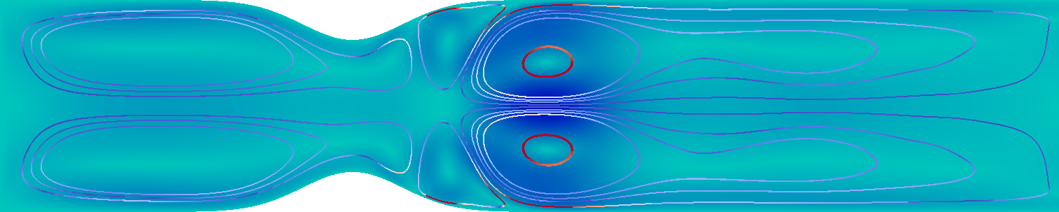
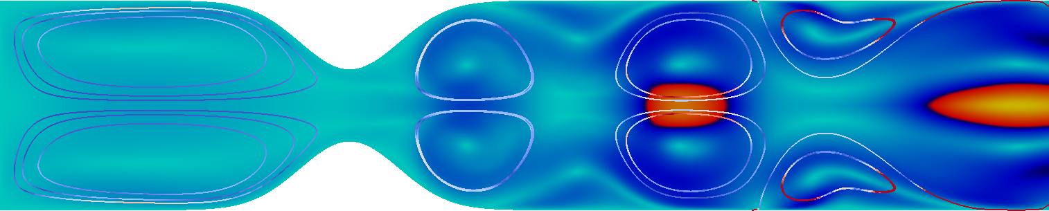
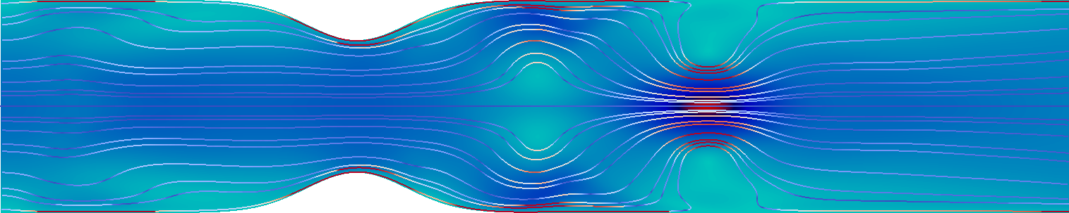
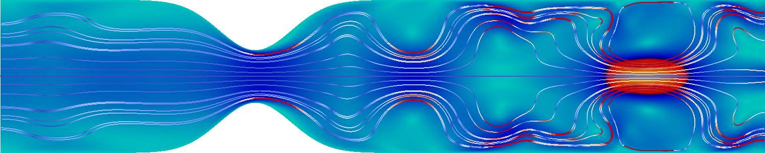
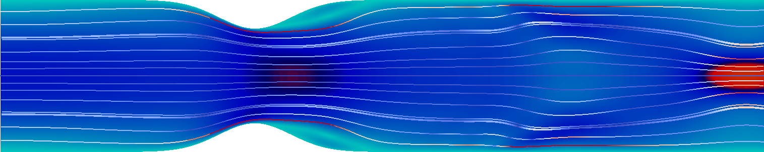
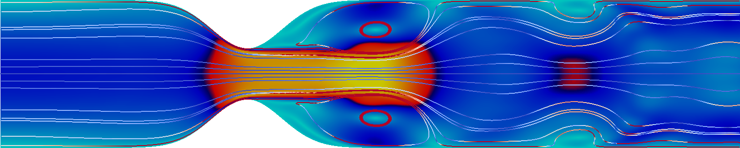
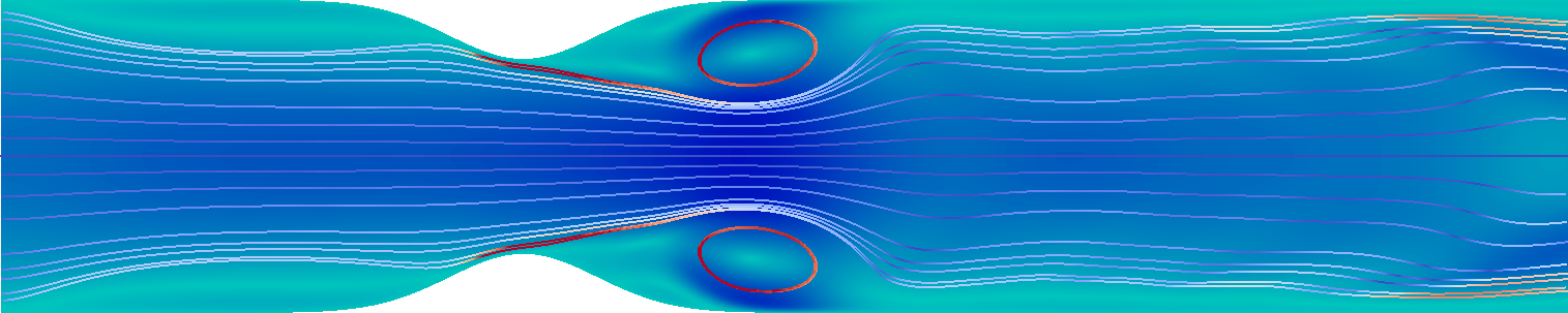
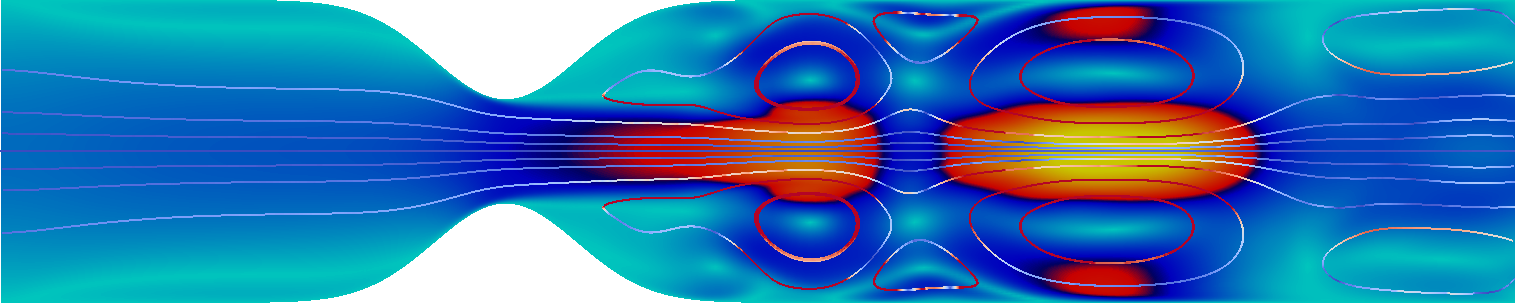
Figure 4: Velocity magnitude at times $t=n\cdot 6\,250$s for $n=1,2,\dots,8$ on domains with different growth. As the inflow profile is periodic, the narrowing of the domain causes a significant change of the flow pattern.

In a first test we take the value $\epsilon=5\cdot 10^{-5}$ in (54). By this choice, the concentration $u$ reaches approximately $1$ after about $50\,000\,\mathrm{s}\approx 1\,\mathrm{day}$ such that we can still resolve the coupled problem in all temporal scales (although the direct simulation still takes a substantial effort). To keep the computational effort within bounds we use a rather coarse spatial discretisation with $320$ elements, resulting in $4\,131$ unknowns of a biquadratic equal-order discretisation for velocities and pressure.

In Figure 3 (left) we give an overview of the temporal evolution of the concentration variable $u_{k}(t)$ using a full resolution of the fast scale. The simulations break down at $T\approx 55\,000\,\mathrm{s}$ due to the deterioration of the ALE map and the high Reynolds number. For the small interval $[10\,000\mathrm{s},10\,002\mathrm{s}]$ we show a close-up view of the resolved solution $u_{k}(t)$ and the averaged value $\int_{t}^{t+1}u_{k}(s)\,\text{d}s$. The deviation is bound by $3\cdot 10^{-6}={\mathcal{O}}\left({\epsilon}\right)$, in agreement with Lemma 3.8. We determine reference values $u_{ref}(T_{n})$ by extrapolating numerical results for $k=0.05\mathrm{s}$, $k=0.025\mathrm{s}$ and $k=0.0125\mathrm{s}$. The relative errors $|u_{k}(t_{n})-u_{ref}(t_{n})|/|u_{ref}(t_{n})|$ (based on these extrapolated errors) are given in Figure 3 (right). The convergence rate in terms of $k$ is approximately quadratic. Further, there is no significant accumulation of simulation errors over time.

By the evolution of the concentration $u$ over time, the computational domain undergoes substantial deformations with a strong narrowing of the flow domain. In Figure 4 we show snapshots of the solution at different time steps, $t\approx 6250s,13500s,18750s,...,50000s$. The narrowing of the gap causes an acceleration of the fluid resulting in a higher Reynolds number flow with a substantial variation in the feedback functional $R(u,\mathbf{v})$ which depends on the wall shear stress.

Multiscale approach

Next, in Figure 5 we show the results obtained with the multiscale method for this relaxed problem with $\epsilon=5\cdot 10^{-5}$. The tolerance for approximating the periodic flow problems is set to

$$\|\mathbf{v}_{U}(1)-\mathbf{v}_{U}(0)\|_{L^{2}(\Omega)}^{2}+\|p_{U}(1)-p_{U}(0)\|_{L^{2}(\Omega)}^{2}<\text{tol}_{P}^{2}\coloneqq 10^{-8}.$$

For each of the three short time step sizes $k=0.05$s, $k=0.025$s and $k=0.0125$s we use long time step sizes ranging from $K=6\,400$s to $K=400$s. In the left plot we compare the solutions for different values of the long time step size $K$. In this (non-logarithmic) plot we see convergence of the results to the corresponding resolved simulation with the same short step size $k=0.025$s. The lower plot shows the corresponding results for a variation of the small step size $k$, while the long scale step size is fixed to $K=400$s. For comparison we show the results obtained with the resolved simulation for these small-step sizes. Again we see convergence of the multiscale scheme towards the resolved scheme.

	$U_{K}$			error (w.r.t. extrapolation)
$k$	$0.05$s	$0.025$s	$0.0125$s	$0.05$s	$0.025$s	$0.0125$s
$K=6400$s	0.8089225	0.8118418	0.8126760	$1.11\cdot 10^{-2}$	$7.55\cdot 10^{-3}$	$6.53\cdot 10^{-3}$
$K=3200$s	0.8122441	0.8153539	0.8162696	$7.05\cdot 10^{-3}$	$3.25\cdot 10^{-3}$	$2.13\cdot 10^{-3}$
$K=1600$s	0.8132730	0.8164325	0.8173319	$5.80\cdot 10^{-3}$	$1.93\cdot 10^{-3}$	$8.35\cdot 10^{-4}$
$K=800$s	0.8135139	0.8166886	0.8175426	$5.50\cdot 10^{-3}$	$1.62\cdot 10^{-3}$	$5.77\cdot 10^{-4}$
$K=400$s	0.8135782	0.8167926	0.8176490	$5.42\cdot 10^{-3}$	$1.49\cdot 10^{-3}$	$4.47\cdot 10^{-4}$
resolved	0.8135999	0.8168226	0.8176928	$5.42\cdot 10^{-3}$	$1.46\cdot 10^{-3}$	$3.93\cdot 10^{-4}$

$$\text{Fit to }U(k,K) =U+C_{k}k^{q_{k}}+C_{K}K^{q_{K}}\qquad U=0.818006\pm 10^{-3}\%$$

$$C_{k}=-1.12\pm 17\%,\quad C_{k} =-6.61\cdot 10^{-10}\pm 34\%,\quad q_{k}=1.85\pm 3.39\%,\quad q_{K}=1.80\pm 2.14\%$$

Table 1: Convergence of the multiscale method at time $T=51\,200\,\mathrm{s}$. We show the values of $U_{K}$ and the error (w.r.t. the extrapolation in $k\to 0$ and $K\to 0$). We compare the results of the multiscale method with the fully resolved forward computation. Finally, we fit the numerical results to the expected convergence behaviour.

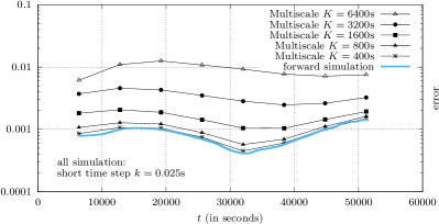
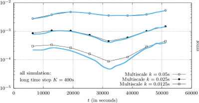
Figure 5: Convergence of the temporal multiscale method for the relaxed problem $\epsilon=5\cdot 10^{-5}$. Left: Effect of the long time step $K$ using the small time step $k=0.025$s. Right: Effect of the short time step $k$ using the long time step size $K=400\mathrm{s}$. For comparison we plot the error of the fully resolved simulation using these time-step sizes.

The effect of the small step size $k$ is dominant. This is highlighted by a closer analysis of the convergence at time $t=51\,200$s, the results being shown in Table 1. We indicate the concentration $U(t)$ and the errors for the different multiscale approaches as well as for the resolved forward simulation. We fit all these values to the postulated relation

$$U(k,K)=U+C_{k}k^{q_{k}}+C_{K}K^{q_{K}}$$ (62)

to get a better understanding of the convergence rates. We estimate all parameters $u,C_{k},C_{K},q_{k},q_{K}$ (obtained with gnuplot fit [48]) and find

$$U(k,K)=U-1.12\cdot k^{1.85}-6.61\cdot 10^{-10}\cdot K^{1.80},$$

see also Table 1. Convergence is close to the expected second order, both in $k$ and $K$. The most striking result is the good estimation of the error constant that shows the proper scaling in $\epsilon^{2}$. This result is in good correspondence to the error estimate derived in Theorem 4.8 where the constant in front of the $K^{2}$-term depends on $\epsilon^{2}$. Balanced discretisation errors are given for $\epsilon^{2}K^{2}\approx k^{2}$, i.e. for $K\approx\epsilon^{-1}k$.

Based on the time step relation we can compute the possible speedup of the multiscale approach which we measure in the overall number of Navier-Stokes time steps to be performed. The forward algorithm requires $E_{fwd}=\frac{T}{k}$ solution steps, while the multiscale approach has an effort of $E_{ms}=\nicefrac{{T}}{{K}}\cdot n_{period}\nicefrac{{1}}{{k}}=\nicefrac{{Tn_{period}}}{{kK}}$ steps, where $n_{period}$ is the number of cycles that are necessary to compute a periodic solution. Given $K\approx\epsilon^{-1}k$ we approximate $E_{ms}\approx\nicefrac{{\epsilon Tn_{period}}}{{k^{2}}}$, and the speedup is estimated by

$$\frac{E_{fwd}}{E_{ms}}=\frac{k}{\epsilon n_{period}}.$$

In our numerical example we identify $n_{period}\leq 5$ and with $\epsilon=5\cdot 10^{-5}$ we expect a speedup of $4\,000k$. In Figure 6 we plot the error over the required number of Navier-Stokes time steps. By circles we indicate the multiscale results with a balanced error contribution, which we define as the state, where the error of the multiscale approach is within $10\%$ of the error of a fully resolved simulation for the same $k$. We observe speedups of 1:250 for $k=0.05\,\mathrm{s}$, 1:180 for $k=0.025\,\mathrm{s}$ and 1:90 for $k=0.0125\,\mathrm{s}$, slightly better values than the predicted ones based on $4000k$. The overall computational time for the forward simulation with $k=0.0125\,\mathrm{s}$ was about 13 days, while the multiscale simulation with $k=0.0125\,\mathrm{s}$ and $K=800\,\mathrm{s}$, giving a comparable accuracy, was about $45\,\mathrm{min}$.

Figure 6: Computational effort (measured in Navier-Stokes times steps) for the multiscale approach (lines) and the resolved forward simulation (points). We use three small time steps $k$ from $0.05$s down to $0.0125$s and vary the long time step $K$ from $6\,400$s to $400$s. Circles indicate multiscale solutions of a quality comparable to the resolved forward simulation (at most 10% additional error). The computational time for one Navier Stokes step is about $0.2$s (Core i7-7700, 3.60GHz, 1370 spatial unknowns, biquadratic finite elements).

5.4.2 Configuration with realistic time scales

Finally, we consider the coupled problem with the time scale parameter $\epsilon=10^{-6}$, which is close to the temporal dynamics of atherosclerotic plaque growth and 50 times smaller than in the first example. Here, a resolved forward simulation is not feasible. The concentration $u(t)$ will reach a value of approximately $0.8$ at $T\approx 2.5\cdot 10^{6}\mathrm{s}\approx 30\,\mathrm{days}$.

	$h=0.16$cm			$h=0.08$cm			$h=0.04$cm
	$k=0.05$s	$k=0.025$s	$k=0.0125$s	$k=0.05$s	$k=0.025$s	$k=0.0125$s	$k=0.05$s	$k=0.025$s	$k=0.0125$s
$K=204800$s	$4.45\cdot 10^{-3}$	$2.46\cdot 10^{-3}$	$2.20\cdot 10^{-3}$	$4.06\cdot 10^{-3}$	$2.42\cdot 10^{-3}$	$2.04\cdot 10^{-3}$	$4.06\cdot 10^{-3}$	$2.42\cdot 10^{-3}$	$2.04\cdot 10^{-3}$
$K=102400$s	$2.86\cdot 10^{-3}$	$8.94\cdot 10^{-4}$	$6.17\cdot 10^{-4}$	$2.75\cdot 10^{-3}$	$1.06\cdot 10^{-3}$	$6.28\cdot 10^{-4}$	$2.75\cdot 10^{-3}$	$1.06\cdot 10^{-3}$	$6.28\cdot 10^{-4}$
$K=51200$s	$2.43\cdot 10^{-3}$	$4.76\cdot 10^{-4}$	$1.96\cdot 10^{-4}$	$2.39\cdot 10^{-3}$	$7.04\cdot 10^{-4}$	$2.58\cdot 10^{-4}$	$2.39\cdot 10^{-3}$	$7.04\cdot 10^{-4}$	$2.58\cdot 10^{-4}$
extrapolated ($k,K\to 0$)		$|U(T)-U_{h}(T)|\approx 4.55\cdot 10^{-2}$		$|U(T)-U_{h}(T)|\approx 8.61\cdot 10^{-3}$			$|U(T)-U_{h}(T)|\approx 1.63\cdot 10^{-3}$

Table 2: Convergence of the multiscale approach for $\epsilon=10^{-6}$. On three mesh levels we indicate the errors in the concentration $U(T)$ at $T=1\,843\,200\,\mathrm{s}\approx 21\,\mathrm{days}$. In each block, the error are given w.r.t. the extrapolation $k,K\to 0$. In the last line we indicate the (dominating) spatial error for each block.

Assuming the validity of estimate (62) and in addition that $C_{K}\approx\epsilon^{2}$ we expect balanced error contributions for $K\approx\epsilon^{-1}k=10^{6}k$. The character of the short scale problem does not depend on $\epsilon$. Hence we consider again the step sizes $k=0.05$s, $k=0.025$s and $k=0.0125$s. The large time step, however, can be significantly increased. We present results for $T\approx 21\,\mathrm{days}$ in Table 2. For this second example, we vary also the mesh size $h$ to discuss the impact of all relevant discretisation parameters. While a smaller value of $\epsilon$ makes the time scale challenge more severe, the multiscale approach will profit, as the potential speedup will benefit from the relation $K\approx\epsilon^{-1}k$.

Figure 7: Left: Error of the multiscale method under refinement in $h,k$ and $K$ versus the extrapolated reference value. Right: Comparison of the computational times of the multiscale method with the corresponding results for a resolved forward simulation. These results are based on an extrapolation of the error and a prediction of the computational times by multiplying the number of required time steps with the average computing times for each step.

Combining all 27 computations based on three values for $h,k$ and $K$ we find the relation

$$U(h,k,K)\approx 0.59076+7.6h^{2.4}-1.7k^{2.2}-0.04\epsilon^{2}K^{1.9},$$

which shows approximately second order convergence in both time step sizes and the mesh size and also the proper scaling of the constants in the ${\mathcal{O}}\left({k^{2}}\right)$ and ${\mathcal{O}}\left({K^{2}}\right)$ terms. Spatial and temporal errors show a different sign which is also seen in Figure 7, where we plot the errors for all computations. In the right sketch of this figure we compare the computational times of the multiscale approach with a hypothetical resolved simulation. Here, the errors are predicted by extrapolation. The computational times are based on the number of Navier Stokes steps, namely $k^{-1}T$ and the average computational time for each Navier Stokes step, which is $0.135\,\mathrm{s}$ on the $h=0.16\,\mathrm{cm}$ mesh, $0.62\,\mathrm{s}$ for $h=0.08\,\mathrm{cm}$ and $2.3\,\mathrm{s}$ for $h=0.04\,\mathrm{cm}$. The results are very similar to those shown in Figure 6 for the first example. The best multiscale results are close to the hypothetical resolved results. Here however, the savings are substantially larger, with 10 minutes vs. 2 months (factor 1:8000) for $h=0.16\,\mathrm{cm}$, 1 hour vs. nearly 2 years for $h=0.08\,\mathrm{cm}$ (factor 1:12000) and 15 hours vs. more than 10 years for $h=0.04\,\mathrm{cm}$ (factor 1:6000).

Finally, we also evaluate the effect of the parameter $\text{tol}_{P}$ used to control the periodicity of the Navier-Stokes solution, compare Theorem 4.8. In Table 3 we show the errors at $T=1\,843\,200\,\mathrm{s}\approx 1\,\mathrm{month}$ for computations based on $K=25\,600\,\mathrm{s}\approx 7\,\mathrm{h}$, $k=0.0125\,\mathrm{s}$ and $h=0.08\,\mathrm{cm}$. The effect of $\text{tol}_{P}$ is very small.

$\text{tol}_{P}$	$10^{-1}$	$10^{-2}$	$10^{-3}$	$10^{-4}$
$\big{|}U_{h,k,K}(T)_{|_{\text{tol}_{P}}}-U_{h,k,K}(T)_{|_{\text{tol}_{P}=10^{-8}}}\big{|}$	$1.99\cdot 10^{-5}$	$4.88\cdot 10^{-7}$	$3.19\cdot 10^{-7}$	$1.22\cdot 10^{-7}$

Table 3: Impact of the periodicity parameter $\text{tol}_{P}$ on the error in concentration $U$ in $T=1\,843\,200$s. Computed with respect to $\text{tol}_{P}=10^{-8}$. The discretisation is chosen as $h=0.08$cm, $k=0.0125$s and $K=25\,600$s.

6 Conclusion

We have presented a framework for the simulation of temporal multiscale problems, where we are interested in the evolution of a slow variable which depends on an oscillating fast variable. The numerical schemes are designed for models that are given by partial differential equations. The most important assumption is a local (in time) proximity of the fast scale variable to the solution of a periodic problem. An effective scheme for the slow variable is derived by replacing the fast variable with the periodic solution which can be computed locally, as no initial values must be transferred. The only overhead of the multiscale scheme comes from the identification of initial values required for approximating the periodic problems. Nevertheless, we gain huge speedups compared to a simulation with resolved time scales. The efficiency of the multiscale approach increases when the time scale separation gets larger.

The resulting scheme depends on several numerical parameters, small and large time steps $k$ and $K$, and the spatial mesh size $h$. It remains a topic for a future work to design an automatic and adaptive algorithm to control all these parameters in order to balance all contributing error terms.

References

- [1] A. Abdulle, W. E, B. Engquist, and E. Vanden-Eijnden. The heterogeneous multiscale method. Acta Numerica, pages 1–87, 2012.
- [2] A. Ammar, F. Chinesta, E. Cueto, and M. Doblaré. Proper generalized decomposition of time-multiscale models. International Journal for Numerical Methods in Engineering, 90(5):569–596, 2012.
- [3] D. Aubry and G. Puel. Two-timescale homogenization method for the modeling of material fatigue. In IOP Conference Series: Materials Science and Engineering, volume 10, page 012113. IOP Publishing, 2010.
- [4] R. Becker and M. Braack. A finite element pressure gradient stabilization for the Stokes equations based on local projections. Calcolo, 38(4):173–199, 2001.
- [5] R. Becker, M. Braack, D. Meidner, T. Richter, and B. Vexler. The finite element toolkit Gascoigne. http://www.gascoigne.uni-hd.de.
- [6] C.L. Bottasso. Multiscale temporal integration. Computer Methods in Applied Mechanics and Engineering, 191(25-26):2815–2830, 2002.
- [7] P. Chakraborty and S. Ghosh. Accelerating cyclic plasticity simulations using an adaptive wavelet transformation based multitime scaling method. Int. J. Num. Meth. Engrg., 93:1425–1454, 2013.
- [8] C.X. Chen, Y. Ding, and J.A. Gear. Numerical simulation of atherosclerotic plaque growth using two-way fluid-structural interaction. ANZIAM J., 53:278–291, 2012.
- [9] V.V. Chepyzhov, V. Pata, and M.I. Vishik. Averaging of 2d Navier–Stokes equations with singularly oscillating forces. Nonlinearity, 22(2):351, 2008.
- [10] Doina Cioranescu and Patrizia Donato. An Introduction to Homogenization. Oxford Lecture Series in Mathematics and its applications. Oxford University Press, 1999.
- [11] R.D. Crouch and C. Oskay. Accelerated time integrator for multiple time scale homogenization. Int. J. Numer. Meth. Engrg., 101:1019–1042, 2015.
- [12] S.S. Dhawan, R.P.A. Nanjundappa, J.R. Branch, et al. Shear stress and plaque development. Expert Rev Cardiovasc Ther., 8(4):545–556, 2010.
- [13] J. Donea. An arbitrary Lagrangian-Eulerian finite element method for transient dynamic fluid-structure interactions. Comput. Methods Appl. Mech. Engrg., 33:689–723, 1982.
- [14] W. E. Principles of Multiscale Modeling. Cambridge University Press, 2011.
- [15] W. E and B. Engquist. The heterogenous multiscale method. Comm. Math. Sci., 1(1):87–132, 2003.
- [16] B. Engquist and Y.-H. Tsai. Heterogeneous multiscale methods for stiff ordinary differential equations. Math. Comp., 74(252):1707–1742, 2005.
- [17] S. Frei, T. Richter, and T. Wick. Long-term simulation of large deformation, mechano-chemical fluid-structure interactions in ALE and fully Eulerian coordinates. J. Comp. Phys., 321:874 – 891, 2016.
- [18] G. P. Galdi and M. Kyed. Time-periodic solutions to the Navier-Stokes equations in three-dimensional whole-space with a non-zero drift term: Asymptotic profile at spatial infinity. arXiv:1610.00677v1, 2016.
- [19] G.P. Galdi and M. Kyed. Time-periodic solutions to the Navier-Stokes equations. In Giga Y., Novotny A. (eds) Handbook of Mathematical Analysis in Mechanics of Viscous Fluids, pages 1–70. Springer, 2016.
- [20] M. Gander and L. Halpern. Techniques for locally adaptive time stepping developed over the last two decades. In Domain Decomposition Methods in Science and Engineering XX, volume 91 of Lecture Notes in Computational Science and Engineering, pages 377–385. Springer, 2013.
- [21] S. Govindjee, T. Potter, and J. Wilkening. Cyclic steady states of treaded rolling bodies. Int. J. Num. Meth. Engrg., 99:203–220, 2014.
- [22] T. Guennouni. Sur une méthode de calcul de structures soumises à des chargements cycliques: l’homogénéisation en temps. ESAIM: Mathematical Modelling and Numerical Analysis, 22(3):417–455, 1988.
- [23] F.M. Hante, M.S. Mommer, and A. Potschka. Newton-Picard preconditioners for time-periodic, parabolic optimal control problems. SIAM J. Numer. Anal., 53(5):2206–2225, 2015.
- [24] S. Haouala and I. Doghri. Modeling and algorithms for two-scale time homogenization of viscoelastic-viscoplastic solids under large numbers of cycles. International Journal of Plasticity, 70:98–125, 2015.
- [25] J. Heywood and R. Rannacher. Finite element approximation of the nonstationary Navier-Stokes problem. i. regularity of solutions and second order error estimation for spatial discretizations. SIAM J. Numer. Anal., 19(2):275–311, 1982.
- [26] J. Heywood and R. Rannacher. Finite element approximation of the nonstationary Navier-Stokes problem. IV. error analysis for second-order time discretization. SIAM J. Numer. Anal., 27(3):353–384, 1990.
- [27] J.G. Heywood, R. Rannacher, and S. Turek. Artificial boundaries and flux and pressure conditions for the incompressible Navier-Stokes equations. Int. J. Numer. Math. Fluids., 22:325–352, 1992.
- [28] T.J.R. Hughes and J.R. Stewart. A space-time formulation for multiscale phenomena. Journal of Computational and Applied Mathematics, 74(1-2):217–229, 1996.
- [29] A.A. Ilyin. Global averaging of dissipative dynamical systems. Rendiconti Academia Nazionale delle Scidetta dli XL. Memorie di Matematica e Applicazioni, 116:165–191, 1998.
- [30] L. Jiang, L. T. Biegler, and V. G. Fox. Simulation and optimization of pressure-swing adsorption systems for air separation. AIChE Journal, 49(5):1140–1157, 2003.
- [31] R.A. Khurram and A. Masud. A multiscale/stabilized formulation of the incompressible navier–stokes equations for moving boundary flows and fluid–structure interaction. Computational Mechanics, 38(4-5):403–416, 2006.
- [32] M. Kyed. Time-periodic solutions to the Navier-Stokes equations. Technische Universität Darmstadt, 2012. Habilitationsschrift.
- [33] J. Lemaitre and I. Doghri. Damage 90: a post processor for crack initiation. Comp. Meth. Appl. Mech. Engrg., 115:197–232, 1994.
- [34] V. Levenshtam. Justification of the averaging method for a system of equations with the navier–stokes operator in the principal part. St. Petersburg Mathematical Journal, 26(1):69–90, 2015.
- [35] Y. Maday and G. Turinici. The parareal in time iterative solver: a further direction to parallel implementation. In Domain decomposition methods in science and engineering, pages 441–448. Springer, 2005.
- [36] A. Masud and R.A. Khurram. A multiscale finite element method for the incompressible Navier–Stokes equations. Computer Methods in Applied Mechanics and Engineering, 195(13-16):1750–1777, 2006.
- [37] J. Mizerski and T. Richter. The candy wrapper problem - a temporal multiscale approach for pde/pde systems. In Numerical Mathematics and Advanced Applications - Enumath 2019, Lecture Notes in Computational Science and Engineering. Springer, 2020.
- [38] O.A. Oleinik, A.S. Shamaev, and G.A. Yosifian. Mathematical Problems in Elasticity and Homogenization, volume 26 of Studies in Mathematics and its Applications. North-Holland, 1992.
- [39] J.-C. Passieux, P. Ladevèze, and D. Néron. A scalable time–space multiscale domain decomposition method: adaptive time scale separation. Computational Mechanics, 46(4):621–633, 2010.
- [40] T. Richter. Goal oriented error estimation for fluid-structure interaction problems. Comput. Methods Appl. Mech. Engrg., 223-224:28–42, 2012.
- [41] T. Richter. Fluid-structure Interactions. Models, Analysis and Finite Elements, volume 118 of Lecture notes in computational science and engineering. Springer, 2017.
- [42] T. Richter. An averaging scheme for the efficient approximation of time-periodic flow problems. submitted, 2019. https://arxiv.org/abs/1806.00906.
- [43] T. Richter and W. Wollner. Efficient computation of time-periodic solutions of partial differential equations. Viet. J. Math., accepted 2018.
- [44] J.A. Sanders, F. Verhulst, and J. Murdock. Averaging Methods in Nonlinear Dynamical Systems, volume 59 of Applied Mathematical Science. Springer, 2007.
- [45] F. Sonner and T. Richter. Optimal pressure estimates for the Crank-Nicolson discretization of the incompressible Navier-Stokes Equations. SIAM J. Numer. Anal., 58(1):375–409, 2020.
- [46] M. Steuerwalt. The existence, computation, and number of solutions of periodic parabolic problems. SIAM J. Numer. Anal., 16(3):402–420, 1979.
- [47] A. Whale, J.J. Lopez, M.E. Oszewski, et al. Plaque development, vessel curvature, and wall shear stress in coronary arteries assessed by x-ray angiography and intravascular ultrasound. Med Image Anal., 10(4):615–631, 2006.
- [48] T. Williams, C. Kelley, and many others. Gnuplot 4.6: an interactive plotting program. http://gnuplot.sourceforge.net/, April 2013.
- [49] Y. Yang. Mathematical modeling and simulation of the evolution of plaques in blood vessels. PhD thesis, Universität Heidelberg, 2014. doi: 10.11588/heidok.00016425.
- [50] Y. Yang, W. Jäger, M. Neuss-Radu, and T. Richter. Mathematical modeling and simulation of the evolution of plaques in blood vessels. J. of Math. Biology, 72(4):973–996, 2016.
- [51] Y. Yang, T. Richter, W. Jäger, and M. Neuss-Radu. An ALE approach to mechano-chemical processes in fluid-structure interactions. Int. J. Numer. Math. Fluids., 84(4):199–220, 2017.
- [52] Q. Yu and J. Fish. Temporal homogenization of viscoelastic and viscoplastic solids subjected to locally periodic loading. Computational Mechanics, 29(3):199–211, 2002.
- [53] M. J. Zahr, P.-O. Persson, and J. Wilkening. A fully discrete adjoint method for optimization of flow problems on deforming domains with time-periodicity constraints. Computers and Fluids, 139:130–147, 2016.