Quantum turbulence in quantum gases

Abstract

Turbulence is characterized by a large number of degrees of freedom, distributed over several length scales, that result into a disordered state of a fluid. The field of quantum turbulence deals with the manifestation of turbulence in quantum fluids, such as liquid helium and ultracold gases. We review, from both experimental and theoretical points of view, advances in quantum turbulence focusing on atomic Bose-Einstein condensates. We also explore the similarities and differences between quantum and classical turbulence. Lastly, we present challenges and possible directions for the field. We summarize questions that are being asked in recent works, which need to be answered in order to understand fundamental properties of quantum turbulence, and we provide some possible ways of investigating them.

1 INTRODUCTION

Turbulence is characterized by a large number of degrees of freedom interacting nonlinearly, over a substantial range of scales, to produce a disordered state both in space and time. Many aspects of classical turbulence (CT) are not well-understood, so tackling its quantum version, quantum turbulence (QT), seems ambitious. It turns out that dealing with turbulence in quantum fluids might be easier than its classical counterpart, due to the fact that the vortex circulation is quantized in the former and continuous in the latter. The advances in trapping, cooling, and tuning the interparticle interactions in atomic Bose-Einstein condensates (BECs) make them excellent candidates for studying QT, due to the amount of control that one can exert over these systems.

[] CTclassical turbulence QTquantum turbulence BECBose-Einstein condensate

Despite the intrinsic difficulties of this problem, much progress has been done [1, 2, 3]. A milestone was the first observation of turbulence in a trapped BEC [4], and its signature self-similar expansion. The occurrence of an energy cascade, demonstrated by the presence of a power law in the energy spectrum $E\propto k^{-\delta}$, can be considered as an important step toward the understanding of turbulence in confined systems [5, 6, 7].

A few words about the scope of this review are in order. In this work we focus on quantum turbulence in trapped BECs. Comparisons with turbulence in liquid helium are made when pertinent, but a full review of the subject is beyond the span of this paper. The same can be said about classical turbulence.

This review is structured as it follows. A very brief introduction to quantum gases is given in Sec. 2. In Sec. 3 we present the main aspects of quantum turbulence. We begin with definitions of “turbulence” and QT, Sec. 3.1. The picture of a tangle of vortices giving rise to turbulence is first introduced in Sec. 3.2. In Sec. 3.3 we contrast aspects of classical and quantum turbulence, with brief accounts of both. Some models that have been used to explore QT, namely the Biot-Savart (BS) and Gross-Pitaevskii (GP) models, are introduced in Sec. 3.4. Wave turbulence is discussed in Sec. 3.5. Section 3.6 deals with one mechanism that is believed to be essential to QT, vortex reconnections. Some aspects of two-dimensional turbulence, which is substantially different from its three-dimensional counterpart, are presented in Sec. 3.7. Section 3.8 contains topics that are not related to the “usual” single-component BECs employed in the study of QT, namely bosonic mixtures and fermionic systems. Section 4 summarizes the experimental achievements, describing important aspects of turbulence observed in quantum gases in 3D and 2D. We emphasize the recent developments in our group, and we show how the experiments performed in our laboratories relate to the research on quantum turbulence that is being performed worldwide. Finally, in Sec. 5 we present some challenges and future issues that, in our opinion, the field must face.

[] BSBiot-Savart GPGross-Pitaevskii

2 QUANTUM GASES

2.1 Bose-Einstein condensates

Bose-Einstein condensation corresponds to the macroscopic occupation of the lowest energy quantum state by the particles of a system. This occurs if the temperature $T$ of the system is cooled below a critical temperature $T_{c}$. Bose-Einstein condensation occurs when the mean interparticle distance $\bar{l}=(\bar{\rho})^{-1/3}$, $\bar{\rho}$ being the number density of $N$ particles in a volume $V$, is comparable to the de Broglie wavelength $\lambda_{\rm dB}=h/(mv)$, where $h$ is Planck’s constant, $m$ is the mass of the atoms, and $v=\sqrt{k_{B}T/m}$ is their thermal velocity, $k_{B}$ being the Boltzmann constant. Imposing $\lambda_{\rm dB}\sim\bar{l}$ implies that a homogeneous gas will undergo a Bose-Einstein condensation at a temperature $T_{c}\sim h^{2}\rho^{2/3}/(mk_{B})$. This simple qualitative argument differs from the accurate result [8] only by a factor of $\approx$ 3.3. The first experimental realizations of Bose-Einstein condensation in dilute gases were achieved in 1995 [9, 10, 11], and currently several laboratories around the world produce BECs on a daily basis. Most of these experiments are performed on inhomogeneous gases in harmonic trapping potentials. Then, the critical temperature [8] is given by $T_{c}=0.15h\bar{\omega}N^{1/3}/k_{B}$, where $\bar{\omega}=(\omega_{x}\omega_{y}\omega_{z})^{1/3}$ is the geometric mean of the three Cartesian trapping frequencies $\omega_{i}$, $i=x,y,z$. Trapping techniques usually employ magnetic fields or optical means. The extremely low temperatures are achieved by laser cooling and evaporation. One feature of experiments with cold atomic gases that led to rapid advances in the field is the ability to control interactions in the systems. The interatomic interactions and trapping potentials can be changed by modifying external parameters, such as the applied electromagnetic fields, with unprecedented control.

2.2 Superfluid helium

Liquid helium was first produced in 1908, and 20 years later scientists noticed that liquid helium had two very distinct phases, He I and He II, with a singularity in the specific heat, called $\lambda$-point, between them [12]. The behavior of liquid He I was the same as regular liquids, whereas He II displayed unusual mechanical and thermal properties at low temperatures. Progress was made with the discovery of superfluidity [13, 14], flow without viscous dissipation, in direct analogy with the lack of resistance in a superconductor.

London was the first to connect He II with Bose-Einstein condensation [15], proposing a macroscopic wave function for the condensed atoms. However, more attention was given to the phenomenological two-fluid model introduced by Tisza [16]. According to this model, liquid He is composed of a normal and a superfluid part, each of them with its own density and velocity field. The normal component behaves as a regular fluid, while the superfluid has no entropy and flows without friction. Later, Landau formalized the model [17], which was successful in explaining a variety of properties and effects in liquid He. However, a major problem with the two-fluid model is that it assumes zero superfluid vorticity, the vorticity being the curl of the velocity field. This is due to the fact that, in the absence of dissipations, the velocity field should be conservative, and thus it can be written as the gradient of a field, and the curl of a gradient is zero ($\boldsymbol{\omega}=\nabla\times\boldsymbol{v}=\nabla\times\nabla\phi=0$). Experiments, however, showed clear indications that the vorticity did not vanish.

2.3 Quantized vortices

Since Bose-Einstein condensation corresponds to the collective occupation of the zero momentum state, then a macroscopic wave function can be used for the $N$ condensed atoms, $\psi(\boldsymbol{r},t)=\sqrt{\rho(\boldsymbol{r},t)}\exp\left[iS(\boldsymbol{r},t)\right]$, where $\rho(\boldsymbol{r},t)=|\psi(\boldsymbol{r},t)|^{2}$ is the condensed density, $S(\boldsymbol{r},t)$ its phase, and the normalization is given by $\int d^{3}\boldsymbol{r}|\psi(\boldsymbol{r},t)|^{2}=N$. The probability current is given by $\boldsymbol{j}=\hbar/(2mi)\left(\psi^{*}\nabla\psi-\psi\nabla\psi^{*}\right)=\rho(\hbar/m)\nabla S$, where we omitted the spatial and time dependencies hereafter for brevity. This is a flux of the density $\rho$ that flows with velocity $\boldsymbol{v}=(\hbar/m)\nabla S$, $\boldsymbol{j}=\rho\boldsymbol{v}$. A consequence is that, when $S$ has continuous first and second derivatives, the velocity field is irrotational, $\nabla\times\boldsymbol{v}=0$. In the presence of a vortex line, a line singularity where $\boldsymbol{v}$ diverges, this does not hold. Thus, a vortex-free velocity field is irrotational.

The circulation $\Gamma$ around a closed path $C$ is given by $\Gamma=\oint_{C}d\boldsymbol{r}\cdot\boldsymbol{v}$. The macroscopic wave function has to be single-valued, which requires the phase to change by $2\pi n$, where $n$ is an integer and it is often called the charge of the vortex, when going around the contour. This gives rise to the quanta of circulation $\kappa=h/m$,

$$\Gamma=\oint_{C}d\boldsymbol{r}\cdot\boldsymbol{v}=\frac{\hbar}{m}2\pi n=n\kappa.$$ (1)

This led Onsager [18] and Feynman [19] to introduce the quantization of the vorticity in superfluid helium. A vortex is an excitation of the system, thus it is a state with higher energy than the ground-state. It can be shown that the energy is proportional to the square of the vortex charge, $E\propto n^{2}$, thus it is energetically favorable to have $n$ single-charged vortices rather than one $n$-charged vortex [20].

3 QUANTUM TURBULENCE

3.1 Nomenclature

The term “quantum turbulence” was first used in 1982 by Barenghi in his Ph.D. thesis [21]. Donnelly and Swanson, who adopted the term in 1986 [22], were responsible for the shift from the commonly used “superfluid” to “quantum” turbulence. This change was not simply a matter of nomenclature, it showed that turbulence had more to do with the quantization of vortices than the lack of viscosity of superfluids. Indeed, experiments later showed that turbulence would decay even in the case of vanishing viscosity. The very pertinent question of where the energy goes if there is no friction was answered by the realization that vortices decay into sound, as seen in experiments with 2D BECs [23] and numerical simulations using the Gross-Pitaevskii equation in 2D [24] and 3D [25].

Having justified the term “quantum turbulence”, we still have to define “turbulence”. A definition that seems to be accepted is a state of spatially and temporally disordered flow, with a large number of degrees of freedom which interact nonlinearly. Usually, by nonlinear interaction we mean the term $(\boldsymbol{v}\cdot\nabla)\boldsymbol{v}$ in the classical Euler equation,

$$\frac{\partial\boldsymbol{v}}{\partial t}+(\boldsymbol{v}\cdot\nabla)\boldsymbol{v}=-\frac{1}{\rho}\nabla p,$$ (2)

where $p$ is the pressure. The nonlinear term arises simply from writing Newton’s second law for the continuum. As we will see, the equation above can be seen as a particular case of the (incompressible) Navier-Stokes equation with zero viscosity.

3.2 From vortices to turbulence

Vortex lines can sustain helical deformations, called Kelvin waves, that move them from a straight orientation. Also, two lines that approach each other can reconnect and form a cusp, which relaxes into Kelvin waves. Disordered combinations of vortex lines can be a manifestation of quantum turbulence, as proposed by Feynman [19]. The subsequent work done by Hall and Vinen [26, 27] motivated the study of QT using ⁴He. The recent progress of QT in the context of trapped BECs came with striking discoveries. For example, under appropriate conditions, statistical properties of classical turbulence may arise. One of them is the Kolmogorov scaling of the energy spectrum ($E\propto k^{-5/3}$), which suggests an energy cascade from large to small length scales. This defines what is called Kolmogorov turbulence, which is found in a specific inertial range as long as there is constant injection of energy at large length scales. This requires a self-similar process in which large bundles of vortices transfer energy to smaller bundles, until the energy reaches a single vortex.

Numerical simulations showed that if QT obeys the energy spectrum of the Kolmogorov turbulence, the vortex tangle contains transient vortex bundles (vortices with the same orientation) together with many random vortices [28]. These structures are responsible for the large scale, small $k$, flows. Although the Kolmogorov scaling has been observed in experiments, these vortex bundles have not. Kolmogorov turbulence has been observed in helium at low and high temperatures, $T\ll T_{c}$ and $T\sim T_{c}$, respectively. At high temperatures, the normal fluid dominates, so CT is expected. However, at low temperatures the situation is more interesting. Energy transfer occurs because of the non-linear term $(\boldsymbol{v}\cdot\nabla)\boldsymbol{v}$ in the Euler equation, Eq. (2). This helps to connect both QT and CT.

A different kind of turbulence, called Vinen turbulence, has been observed in experiments [29] and numerically [30]. This kind of turbulence is set apart from Kolmogorov’s because of the absence of large-scale flow structures. The question of whether turbulence in trapped BECs is Kolmogorov, Vinen, a combination of both, or neither, is still unsettled. However, two vortices in an orthogonal orientation or one doubly-charged vortex may decay and display a Kolmogorov energy spectrum [31]. Numerical models using the GP equation also suggest that trapped BECs should show Kolmogorov turbulence [32].

One last distinction should be made. Stationary turbulence in 3D (2D) systems requires constant energy injection in large (small) length scales, which cascades to small (large) scales and is dissipated with the same rate as injected. In nature, stationary turbulent systems decay when the energy input stops, characterizing what we call decaying turbulence.

3.3 Brief introductions

3.3.1 Classical versus quantum turbulence

One of the most important differences between classical and quantum turbulence is the quantization of the circulation, see Sec. 2.3. In this sense, the quantum version of the problem is easier to handle due to the fact that circulation, which is continuous in the classical case, can only take a discrete set of values. Regular fluids are viscous, thus, without a constant energy input, turbulence decays. At sufficient low temperatures, the thermal component of the trapped gases is negligible, and it can be considered a pure superfluid. Even in that scenario, turbulence will decay without constant energy injection, due to sound waves inside and at the surface of the condensate.

Trapped BECs also show some interesting features regarding the amount of control exerted on experiments. The number of atoms, trapping parameters, and interatomic interactions can be varied to produce the desired regimes. The drawback is that this freedom often complicates the comparison between two sets of experiments.

The characteristic length scales are different when we compare CT and QT and, moreover, the range available in each case also differs. In classical fluids, vortices can be as large as the typical length scale of the system $D$. For a typical BEC the vortex core is comparable to the healing length $\xi$, and the distance between the vortices is a few times $\xi$.

3.3.2 Classical turbulence

The generalization of Euler’s equation, Eq. (2), is the Navier-Stokes equation. In the case of a solenoidal incompressible fluid it can be written as

$$\frac{\partial\boldsymbol{v}}{\partial t}+(\boldsymbol{v}\cdot\nabla)\boldsymbol{v}=-\frac{1}{\rho}\nabla p+\nu\nabla^{2}\boldsymbol{v}+\boldsymbol{g}\text{ and }\nabla\cdot\boldsymbol{v}=0,$$ (3)

where $\boldsymbol{g}$ stands for the external forces. Reynolds studied the transition from laminar to turbulent flows in a pipe. He found that the transition required the Reynolds number $Re=vD/\nu$, which quantifies the intensity of the turbulence (where $v$ is the flow velocity at a length scale $D$, and $\nu$ is the kinematic viscosity of the fluid), and it can be seen as the ratio of inertial to viscous forces.

The concept of energy cascade came in the 1920s with Lewis Richardson, who knew that a turbulent steady state required a constant energy injection at large length scales, and the energy to be dissipated with the same rate at small length scales. The intermediary range, called inertial range, was characterized by being independent of the viscosity. In the 1940s, Kolmogorov formalized the concept of an energy cascade with a self-similar behavior of the turbulent flow. In the simplest case of an isotropic and homogeneous steady state, the energy goes from the largest length scale $D$ to the smallest one $\eta$, with a constant dissipation rate $\varepsilon$. The Reynolds number connects these lengths scales, $\eta/D\approx Re^{-3/4}$. Kolmogorov suggested that some aspects of turbulence are universal. Instead of working in real space, it is convenient to go to the momentum space, to describe the cascade as a function of wavenumbers $k=2\pi/r$. In the inertial range Kolmogorov showed that the kinetic energy is given by

$$E_{k}=C\varepsilon^{2/3}k^{-5/3},$$ (4)

where $C$ is dimensionless and of order one.

Kolmogorov’s law, Eq. (4), describes three-dimensional flow. There are only a few examples of physical systems where flow is truly 2D, in most cases two-dimensional flow is used as an approximation to a 3D problem, or as building blocks to anisotropic turbulence in 3D. Nevertheless, 2D classical turbulence is completely different from its 3D counterpart. In 1967 Kraichnan showed that, in 2D, the energy flows from small to large length scales, in the opposite direction of the three-dimensional case. The same exponent, $E\propto k^{-5/3}$, is found, but due to an inverse energy cascade (IEC). This occurs simultaneously with a forward cascade of the enstrophy, a quantity that measures the variance of the vorticity, which makes the energy spectrum $E\propto k^{-3}$ for large momenta. [] IECinverse energy cascade

3.3.3 Quantum turbulence

The visualization of the tangle of vortex lines that constitute turbulence in a trapped BEC is very difficult, thus much of the progress has been done relying on numerical simulations. In liquid He experiments, the determination of the vortex line density $L$ is more straightforward, and it can be used as a measure of both the intensity of the QT and the distance between vortices $l\approx L^{-1/2}$.

Not all turbulent states that have been studied correspond to the Kolmogorov scaling. They can be of the Vinen kind [33], but it also depends on how the excitations are performed. If the superfluid is thermally driven, then it lacks energy at the largest scales and it displays $E\propto k^{-1}$ for large momenta [34]. On the other hand, if the superfluid is driven by a turbulent normal fluid, then the energy spectrum is $E\propto k^{-5/3}$ as is the case for Kolmogorov turbulence [34]. Panel (a) of Figure 1 shows a vortex tangle in a homogeneous condensate, obtained from simulations [1], while the Kolmogorov scaling is shown in panel (b).

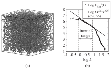
Figure 1: (a) Vortex tangle. (b) Spectrum of the incompressible kinetic energy for the turbulent regime. The points correspond to an ensemble average of 50 configurations, while the curve stands for the Kolmogorov law. Source: Ref. [1].

As we have been arguing throughout this review, one of the reasons for the complexity of QT comes from the large range of length, or conversely momentum, scales available. For the following discussion let us define $k_{l}=2\pi/l$ and $k_{\xi}=2\pi/\xi$, wavenumbers corresponding to the intervortex distance and healing length, respectively. The discussions, so far, were restricted to the hydrodynamical scale $k\ll k_{l}$. Now let us focus on the range $k_{l}<k<k_{\xi}$, $k_{\xi}$ being the limiting scale because vortices cannot bend on scales shorter than the vortex core radius, of order of $\xi$. It is understood that Kelvin waves produce increasingly shorter wave lengths until the angular frequency of the wave is fast enough to radiate sound, in a process called Kelvin cascade. Different theories exist for the energy spectrum of this cascade, Kozik and Svistunov [35] obtained $E\propto k^{-7/5}$, while L’vov and Nazarenko [36] predicted $E\propto k^{-5/3}$. It is still unclear which of the exponents is correct, however recent studies [37, 38, 39] seem to support the spectrum proposed by L’vov and Nazarenko. Another possibility is that there is a bottleneck between the Kolmogorov and Kelvin cascades, which changes the shape of the energy spectrum around $k\approx k_{l}$ [40]. This effect is due to the faster rate at which energy flows in the three-dimensional Kolmogorov cascade, compared to the one-dimensional Kelvin cascade. A different approach, but supposing a smooth transition between the two cascades, has been suggested [41, 42].

3.4 Theoretical models

3.4.1 The Biot-Savart model

First introduced by Schwarz [43], the Biot-Savart model parametrizes the vortex line by the curve $s(\zeta,t)$, $\zeta$ being the arclength and $t$ the time. Its name is due to the analogy with magnetic fields. In this model, the velocity is written as the curl of a vector potential $\boldsymbol{A}$, $\boldsymbol{v}=\nabla\times\boldsymbol{A}$. The vorticity then obeys the Poisson equation, $\nabla^{2}\boldsymbol{A}=-\boldsymbol{\omega}$, with a solution given by

$$\boldsymbol{A}(\boldsymbol{r})=\frac{1}{4\pi}\int d^{3}\boldsymbol{r}^{\prime}\frac{\boldsymbol{\omega}(\boldsymbol{r}^{\prime})}{|\boldsymbol{r}-\boldsymbol{r}^{\prime}|},$$ (5)

for a vortex core located at $\boldsymbol{r}$. The vorticity has a constant intensity along the vortex core, hence $\boldsymbol{\omega}(\boldsymbol{r}^{\prime})d^{3}\boldsymbol{r}=\kappa d\boldsymbol{\ell}$, which allows the integration to be performed over a line, $1/(4\pi)\int d\boldsymbol{\ell}\ \kappa/|\boldsymbol{r}-\boldsymbol{r}^{\prime}|$. Notice that $\boldsymbol{A}$ describes an incompressible field, $\nabla\cdot\boldsymbol{v}=\nabla\cdot\nabla\times\boldsymbol{A}=0$, however a quantum fluid may have a compressible part which is not described in this model. Simulations employing this vector potential are computationally expensive. Instead, the velocity field may be replaced by $\boldsymbol{v}_{\rm LIA}=(\kappa/4\pi R)\ln(R/\zeta)(\boldsymbol{s}^{\prime}\times\boldsymbol{s}^{\prime\prime})$, where the primes stand for derivatives taken with respect to the arclength, $s^{\prime}=ds/d\zeta$ [44]. This is called local induction approximation due to the fact that nonlocal contributions to the integral are neglected. Vortex reconnections, first introduced in Sec. 3.2, and discussed in Sec. 3.6, are essential for QT simulations. These are absent in the BS model and need to be included ad hoc [43, 44].

The BS model may be useful for some qualitative behavior of turbulent quantum fluids, but its assumption of point-like vortex cores, and the absence of explicit vortex reconnections are severe drawbacks. In dilute BECs, where during the expansion a single vortex core may be comparable to the dimension of the whole condensate, this model is not expected to be successful.

3.4.2 The Gross-Pitaevskii equation

The GP approximation was formulated independently by Gross [45] and Pitaevskii [46] in 1961. The key assumption of this mean-field model is that all particles are in the same quantum state, corresponding to zero momentum. Thus the whole system can be described by a macroscopic wave function $\psi(\textbf{r},t)$, which can be found by solving

$$i\hbar\frac{\partial\psi(\textbf{r},t)}{\partial t}=\left[-\frac{\hbar^{2}}{2m}\nabla^{2}+V_{\rm trap}+g|\psi(\textbf{r},t)|^{2}\right]\psi(\textbf{r},t).$$ (6)

The parameter $g=4\pi a_{s}\hbar^{2}/m$ measures the strength of the interaction, and it is proportional to the $s$-wave scattering length $a_{s}$, while the normalization is given by $\int d^{3}\boldsymbol{r}|\psi|^{2}=N$. Although the GP model is a mean-field approach, in the limit of a $T=0$ dilute condensate with two-body repulsive interaction potentials, the GP equation is exact [47, 48].

Contrary to the BS model, vortex reconnections are present in the solutions, and do not have to be included ad hoc. The GP equation has been used successfully to describe a variety of scenarios [49], and dissipation effects can also be included in it [50]. Finally, we should note that methods beyond a mean-field approach are available [51, 52, 53, 54]. A survey on simulations using the GP model, and several other numerical methods applied to QT, can be found in Ref. [55].

We can perform a Madelung transformation to $\psi(\textbf{r},t)$ so that $\psi(\textbf{r},t)=f(\boldsymbol{r},t)\exp\left[iS(\textbf{r},t)\right]$, where the real functions $f$ and $S$ are associated with the square root of the density and phase of the wave function, respectively. Substituting this into Eq. (6) yields two equations, corresponding to the real and imaginary components [8],

$$\frac{\partial f^{2}}{\partial t} = -\frac{\hbar}{m}\nabla\cdot(f^{2}\nabla S),$$ (7)

$$-\hbar\frac{\partial S}{\partial t} = -\frac{\hbar^{2}}{2mf}\nabla^{2}f+\frac{1}{2}mv^{2}+V_{\rm trap}+gf^{2},$$ (8)

with $v=|\boldsymbol{v}|=|\hbar\nabla S/m|$. Equation (7) is the continuity equation with $\rho=f^{2}$ and $\boldsymbol{j}=\hbar f^{2}\nabla S/m$, which shows that the probability $|\psi|^{2}$ is conserved. The gradient of Eq. (8) yields

$$\frac{\partial\boldsymbol{v}}{\partial t}=-\frac{1}{m\rho}\nabla p-\frac{1}{2}\nabla v^{2}+\frac{1}{m}\nabla\left(\frac{\hbar^{2}}{2m\sqrt{\rho}}\nabla^{2}\sqrt{\rho}\right)-\frac{1}{m}\nabla V_{\rm trap},$$ (9)

where we identified $p=\rho^{2}g/2$. Only one term contains $\hbar$, and it is referred to as quantum pressure, which dominates its classical counterpart only for distances of the order of (or less than) the healing length. Neglecting this term yields the dissipation-free Navier-Stokes equation, Eq. (3) with $\nu=0$. It has been pointed out [56] that $S$ is a multivalued field, thus the chain rule of differentiation cannot be applied to $\exp[iS]$. Indeed, the curl of Eq. (9) would lead us to believe that vorticity has no dynamics, $\partial\boldsymbol{\omega}/\partial t=0$. In Ref. [56], the author derives exact hydrodynamic equations which present superfluid behavior and include vorticity dynamics.

3.5 Wave turbulence

So far we talked about turbulence as a result of the motion and interaction of vortices. However, some processes in BECs involve interacting dispersive waves giving rise to turbulence, such as is the case of sound waves. We associate the term wave turbulence (WT) to these type of phenomena. This process also appears as a power law cascade in the energy spectrum [57]. When the equations of motion describe weakly nonlinear dispersion, an analytical description is possible [58]. Sound waves are small amplitude excitations to a macroscopic wave function of the condensate. Keeping only the smallest nonlinearity [59] it is possible to analyze plane-wave solutions and their nonlinear corrections [60]. The result is a three-wave process which allows the existence of a steady state characterized by an energy cascade [58, 61]. In the long wavelength regime, the energy spectrum is of the Zakharov-Sagdeev type, $E\propto k^{-3/2}$ [58]. [] WTwave turbulence

Wave turbulence may also arise from the vibratory motion of vortex lines, known as Kelvin waves. The first theory formulated to explain this type of phenomena involved a six-wave process [35]. Later, Nazarenko pointed out that two different cascades can occur simultaneously in WT, as long as an even number of waves are involved [58]. A direct energy cascade flows from large to small length scales, and there is also an inverse wave action. Within the Kozik-Svistunov theory [35], $E\propto k^{-7/5}$ for the direct process, while $E\propto k^{-1}$ for the inverse action. Kelvin waves occur in classical and quantum fluids [35, 62]. In trapped BECs, they have been observed as the result of the decayment of quadrupole modes [63]. Studies suggests that they may be responsible for the energy transfer between the scales of intervortex separation down to vortex core sizes [64, 65, 66]. This feature is present in simulations [65] using the BS model, see Sec. 3.4.1, which does not include a compressible velocity field. The conclusion is that the cascade enabled by Kelvin waves involves only vortex energy, independently of phonons or other collective modes.

3.6 Vortex reconnections

Experiments with BECs generate a large number of vortices that reconnect and tangle with each other [4, 67]. Many experimental techniques for the creation of vortices in dilute BECs are available [68, 69]. A vortex reconnection (VR) corresponds to the approximation of two vortex lines, which then connect and exchange tails. They are largely responsible for the energy transfer between different scales, thus VRs are of great importance to the study of QT [70]. In Ref. [56] it is shown that the creation or annihilation of a pair of touching vortex lines obeys the power-law $x\propto t^{1/2}$, where $x$ is the distance between the lines and $t$ is the time, which has also been observed in experiments [71] and simulations [72]. In liquid He, VRs have been observed in detail [73], whereas the observation in trapped BECs is much more recent [74]. Vortex reconnections release kinetic energy and they concentrate vibrations on individual vortex cores, which in turn can be carried by helical Kelvin waves. This is related to an open question in the heart of QT, the mechanism behind dissipation of $T=0$ frictionless fluids [64]. Vinen proposed that high frequency oscillations of a vortex core can produce phonons in order to dissipate energy in an inviscid fluid [75]. [] VRvortex reconnection

3.7 Quantum turbulence in 2D

We already mentioned that classical turbulence in 2D is very different from the 3D case. Unlike the classical case, where the 2D character is often an approximation to a 3D problem, truly two-dimensional systems can be realized with BECs by exploring the experimental control on the trapping potentials. This makes dilute cold gases the ideal systems to study two-dimensional QT (2DQT) [2]. Kelvin waves, the cornerstone for QT decayment in 3D, are not present in 2D, since vortices are zero-dimensional objects in a plane. [] 2DQT two-dimensional quantum turbulence

The incompressible kinetic energy spectrum of the 2D turbulent regime, for a quasiclassical system with a relatively large $D/\xi$, is given by $E\propto k^{-3}$ for $k\gg 1/\xi$, and $E\propto k^{-5/3}$ for $k<1/\xi$ [76]. In Sec. 3.3.2 we stated that the classical energy spectrum is proportional to $k^{-3}$ for lager momenta due to a direct enstrophy cascade. Although in the quantum case the exponent is the same, the mechanism behind it is completely different. The $k^{-3}$ scaling is the result of the velocity field profile of the quantized vortices, which are also responsible for the enstrophy to be proportional to the number of vortices [2, 76]. The possibility of a vortex-antivortex pair annihilation makes the enstrophy not to be an inviscid quantity. This feature of fluctuating number of vortices is highlighted in GP simulations of Ref. [77]. Another study employed simulations of a purely incompressible fluid and found that the IEC takes place only for systems with moderate dissipation [78]. Further evidence for the IEC includes dynamical simulations of a forced homogeneous systems where the $k^{-5/3}$ scaling was observed, and also clusters of vortices with the same sign [79].

The first investigations of QT in BECs looked for quasiclassical characteristics [80]. Unlike the homogeneous case, trapped BECs tend to prevent large scale motion, so that Vinen turbulence is usually observed. For example, in Ref. [81] the stirring of a BEC, which was happening at distances of the order of the healing length, was unable to produce the growth of vortex clustering due to the system size. When the Kolmogorov scaling can be seen, usually it is for regions less than a decade [82], again due to the lack of range of scales available.

Another obstacle to observing QT in 2D is the vortex-antivortex pair annihilation, which largely prevents vortex clustering. Experimental protocols for vortex generation end up producing roughly the same number of positive and negative charge vortices [23, 67, 83]. Techniques for successive nucleation of vortices have been proposed [84]. Results of simulations in a large, homogeneous BEC clearly show that vortex annihilation is a four-vortex process [85].

3.8 Miscellanea

3.8.1 Bosonic mixtures

So far we limited ourselves to the discussion of single-component BECs. However, QT can also be studied in a mixture of two (or more) bosonic species, with substantially different behavior. Theoretical investigations of counterflow turbulence have been carried out employing a mixture of two bosonic species [86, 87]. This would be the analog of QT in ⁴He at sufficiently high temperatures, when both the normal and superfluid components are turbulent. Quantum turbulence can also be studied using condensates with particles possessing a spin degree of freedom [88, 89]. The main difference to a regular mixture of bosonic species is that the population of each spin state is not constant, due to spin-exchange collisions. For more details about spin turbulence, the reader is referred to Ref. [90] and references therein.

3.8.2 Fermionic gases

Superfluidity can also be achieved in fermionic systems, which is explained thorough the Bardeen-Cooper-Schrieffer (BCS) theory of condensation of Cooper pairs into bosonic-like particles [91]. Interest in cold atomic fermionic gases is further augmented by the BEC-BCS crossover [92], where the interparticle interactions can be tuned so that the fermion pairs can change their size from tightly bound dimers (BEC) to many times the interparticle distance at the BCS side, passing through the strongly-interacting unitary regime. A landmark was the production of vortex lattices, throughout the crossover, in an ultracold ⁶Li gas, demonstrating superfluidity [93]. The first question that arises is if QT is possible in fermionic gases and, if so, in which regimes of BEC-BCS crossover turbulence emerges [94]. Apparently, QT is possible in the unitary Fermi gas [95], and vortex reconnections were studied in this regime [96]. The microscopic structure of vortices in cold atomic fermionic gases has been studied throughout the BEC-BCS crossover and in the unitary Fermi gas [97, 98]. [] BCSBardeen-Cooper-Schrieffer

3.8.3 Neutron stars

Many problems in nuclear physics are related to quantum turbulence. Since protons and neutrons are spin-1/2 particles, QT of fermionic gases is of interest. In particular, QT may hold the key to a mystery in nuclear astrophysics, the pulsar glitches. They correspond to sudden increases in the spinning of neutron stars, while they continually lose angular momentum. It has been suggested that the outer core of a neutron star is in a turbulent state, and that the Reynolds number is related to the glitches [99, 100]. The main challenge in this problem is the disparity between the femtometer scale of vortex cores and the kilometer scale of neutron stars, however progress has been made towards developing a mean field description [101]. As is the case with turbulence in trapped BECs, we need a better understanding of microscopic processes, such as vortex reconnections, that take place in the crust of neutron stars. Even the study of a single vortex line in neutron matter is an active topic of research [102].

4 EXPERIMENTS

The study of quantized vortices and QT has increased in intensity with the realization of weakly interacting dilute atomic BECs [9, 11]. Stimulated largely by the high degree of control which is available within these quantum gases [103, 104, 105, 106], they have been used to investigate quantum turbulence both experimentally and theoretically. The ability to directly resolve the structure of individual vortices and hence the dynamics of a turbulent vortex tangle [63, 64, 74], opens the possibility of studying problems which may be relevant to our general understanding of turbulence.

4.1 The São Carlos Group

We start by reviewing some of our contributions, both theoretical and experimental, to the field of quantum turbulence, and we show how they are related to research being conducted worldwide. In 2009, the São Carlos group was responsible for the first evidences of quantum turbulence in trapped dilute atomic BECs [4]. The experiment consisted of a small vortex tangle created in a harmonically trapped BEC through the combination of rotation and an external oscillating perturbation [4, 107].

Different regimes were observed according to the strength and duration of the external oscillatory potential [5], Figure 2. For small amplitude excitations, the only effect was a bending of the main axis of the cloud, irrespective of the duration of the oscillation. Increasing the amplitude of the oscillation caused regular vortices to be nucleated, with the number of vortices increasing monotonically with the application time of the external excitation. Increasing the excitation time further led to a turbulent vortex regime. At very long hold times, the condensate fragmented or granulated, signalizing the decay of the turbulence.

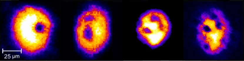
(a) Regular vortices

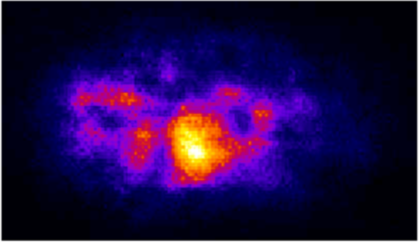
(b) Turbulence

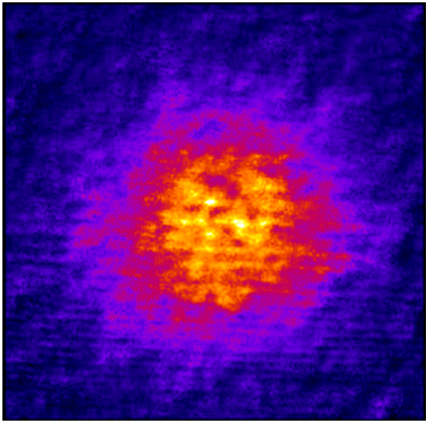
(c) Granulation

Figure 2: Phases of the excited BEC, according to the time and amplitude of the applied external oscillatory magnetically field. From left to right: (a) regular vortices, (b) turbulent cloud, and (c) granulation. Figures extracted from Ref. [108].

4.1.1 Finite size system

Currently, the BEC systems which can be created in the laboratory contain a small number of atoms (a few hundred thousand), and hence do not sustain the number of quantum vortices present in helium experiments. This brings to light the question about the Kolmogorov’s scaling, if it still holds in the small range of lengths available. Despite of the limited number of vortices present in trapped BECs, numerical simulations of these systems [66, 109, 110, 111] suggest that the kinetic energy is distributed over the length scales in agreement with the $k^{-5/3}$ Kolmogorov scaling observed in ordinary turbulence.

Attempts to model analytically the transition to turbulence in these finite systems are available in the literature. The transition from vortices to the turbulent regime could be established assuming a critical number of vortices, according to the size of the sample [112] and to the input energy coming from the external excitation. In Ref. [113], the authors performed numerical calculations to reproduce our experimental conditions. According to the excitation parameters, the perturbed system was classified by a phase diagram. Particular aspects of the granular phase were explored [114].

4.1.2 Self-similar expansion

The most common diagnostic of trapped atomic clouds is done by imaging them, not in the trap, but after some time of free expansion. That easily distinguishes a thermal from a Bose-condensed cloud. A thermal cloud shows a gaussian density profile that evolves to an isotropic density distribution at long times of expansion. The quantum cloud, in contrast, shows a profile that initially reflects the shape of the confining trap, the Thomas-Fermi regime. In a cigar-shaped trap, for example, the BEC cloud expands faster in the radial than in the axial direction. That causes the signature inversion of the BEC cloud aspect-ratio during the free expansion.

Considering now a turbulent BEC cloud, besides the evidences of the tangle vortices configuration in the density profile (atomic depletion in the absorption image), the cloud free expansion dynamics also differs due to the presence of vorticity. In fact, for the cigar shape trap used in Ref. [4], the turbulent condensate expands with a nearly constant aspect-ratio once released from its confinement.

To characterize the anomalous expansion of the turbulent sample, a generalized Lagrangian approach was applied in Ref. [115]. The kinetic energy contribution of a tangle vortex configuration was added to the system Lagrangian, and the resulting Euler-Lagrange equations described the dynamics of the cloud.

4.1.3 Atomic-turbulence and speckle-fields

Bose-Einstein condensates and atom lasers are examples of coherent matter-wave systems. On the other hand, an optical speckle pattern can be created by the mutual interference of many light waves of the same frequency, with different amplitudes and phases, giving rise to a random light map. A very interesting work [116] draws a parallel between a ground-state/turbulent BEC with the propagation of an optical Gaussian beam/elliptical speckle light map.

The researchers analyzed mainly two characteristics of the spatial disorder of the systems. First, measurements of the aspect ratios of regular and turbulent BECs were performed. It is known that for standard BECs there is an inversion of the aspect ratio of the cloud in time-of-flight (TOF) measurements, whereas in the turbulent case there is a self-similar expansion, without ever inverting its aspect ratio [115]. For a coherent Gaussian beam, there is an inversion of the aspect ratio of the waists, whereas it is preserved in the propagation of the elliptical speckle light map, just as it is the case with the BEC counterparts. The second property that was investigated was the coherence in both systems. It was found that the correlations in regular BECs resemble the ones in the Gaussian beam, while the same is true for the turbulent BEC and speckle beam pair. This duality opens the possibility of improving our understanding of QT by looking at statistical atom optics. [] TOFTime-of-flight

4.1.4 Momentum distribution of a turbulent trapped BEC

To investigate turbulence experimentally, atoms are held for tens of miliseconds in the trap, after the drive has been terminated, and then they are released for imaging. The atoms are measured by a TOF absorption image technique. In Ref. [6], TOF was used to probe the momentum distribution of a turbulent BEC cloud, assuming a ballistic expansion for the atoms. They found a power-law behavior for the momentum distribution of $n(k)\propto k^{-2.9}$, Figure 3.

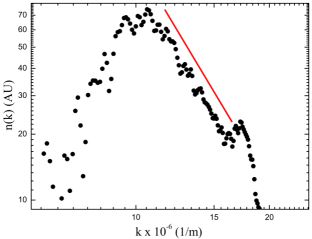
Figure 3: Three-dimensional momentum distribution for a turbulent cloud from Ref. [6]. The curve corresponds to a line with slope -2.9.

The momentum distribution is extracted from measurements of the absorption image of the expanded cloud. The projected image is a distorted two-dimensional shadow of the real atomic distribution. As a result, the spatial density has contributions from many wavenumbers along the path of the imaging light. As the interaction is assumed to be negligible, the ballistically expanding atoms allow for an experimental Fourier conversion of the real space density distribution after a TOF to an $in\,situ$ momentum distribution. The radii of the expanded cloud are converted in momentum shells, and the number of atoms are counted in each shell to construct the momentum distribution of the sample.

Remarkably, the turbulent spectra showed a higher-momentum atomic population that is not present in the spectra of a normal BEC. In particular, this unusual region of the spectra showed a distribution which decreases monotonically with the momentum, and its slope in a logarithmic scale can be associated to a power law.

4.1.5 Collective Modes, Faraday Waves, and Granulation

In Ref. [117], a gas of ⁷Li atoms was cooled to nearly zero temperature, and the collective modes of an elongated BEC were studied with the modulation of the atomic scattering length. Different regimes appeared by varying the frequency and modulation strength of the external magnetic field. This was explored further, both experimentally and theoretically, in Ref. [118]. Particularly, for modulation frequencies near twice the trap frequency, longitudinal surface waves are generated resonantly (parametrically). The dispersion of these waves, also called resonant [119] or Faraday waves [120, 121], is well-reproduced by a mean-field theory. Otherwise, far from the resonances (lower modulation frequencies), increasing the modulation strength brings an irregular granulated distribution in the condensate density, Figure 4. The correlations of this granulated phase could be described with a beyond mean-field theory [122], which characterizes the large quantum fluctuations of this peculiar regime.

Figure 4: Response of an elongated Bose-Einstein condensate to modulated interactions: (a) experiment and (b) numerical simulations. Granulation is remarkably persistent in time after the modulation is turned off, and its structure is random between different experimental runs. Source: Ref. [118].

4.2 Two-dimensional quantum turbulence

Since there is a lack of experimental correspondence, previous numerical studies on 2DQT, which dealt with the energy spectra and vortex dynamics, did not establish any connection with classical 2D turbulence. Recently, the experiments [123, 23] showed that even a trapped superfluid sample exhibits many similarities to what is expected from the 2D classical turbulence, extending the universality of 2D turbulence.

To experimentally generate 2DQT, a combined optical-magnetic confinement creates highly oblate BEC, with the turbulent flow resulting from the effective stirring of the center region of the condensate by a repulsive optical potential. This external perturbation induces randomly distributed nucleation of vortices. Then the trap is turned off, and the expanded BEC provides the absorption image of the vortices.

In Ref. [123], the authors investigated, experimentally and numerically, the forced and decaying 2DQT in a BEC. It was demonstrated that the disordered vortex distributions of 2DQT can be sustained, in spite of the vortex-antivortex annihilation. Their observations are indicators of the energy transport from small to large length scales, corresponding to the inverse energy cascade. The thermal relaxation of superfluid turbulence in 2D, based on evidences of the vortex-antivortex annihilation mechanism, was investigated in Ref. [23]. They showed the essential role played by vortex-antivortex pairs in 2DQT, characterizing the relaxation of the turbulent condensate through the decay rates of the vortex number.

5 CHALLENGES AND OPEN QUESTIONS

Trapped superfluid Bose-Einstein condensates show turbulent behavior. Evidences of energy cascades with power law behavior have been measured in experiments and supported by theoretical models. The amount of control that can be exerted on BEC experiments makes them excellent candidates to investigate quantum turbulence. Nevertheless, several aspects of this phenomenon need experimental investigation and theoretical clarification. In the following we summarize some of the challenges that the field must face.

Tuning the interactions: Throughout this manuscript we pointed out several limitations due to the range of available length scales in experiments. A quick estimate of $\log(D/\xi)$, involving the system size $D$ and the healing length $\xi$, shows that experiments are limited to one or two decades at best. However, interactions in trapped BECs can be controlled through Feshbach resonances [103] to produce smaller healing lengths and larger cloud radii at the same time, improving the range of scale lengths available. How turbulence formation, decay and scaling laws, would react in different interacting environments? Many other questions could be investigated as one studies turbulence in tunable BECs.

Finite size: Currently, the dilute BECs which can be created in the laboratory contain a small number of atoms, hence do not sustain the number of quantum vortices present in helium experiments. Fundamental questions exist over the extent to which turbulence can be generated and observed in such small and inhomogeneous systems.

Inhomogeneity: Trapped quantum gases are not homogeneous systems. What is the influence of this on characteristics of QT in these systems? Following the release of the trap, turbulence is expected to be isotropic after a sufficiently long time. However, experiments are limited to images a few tens of milliseconds after the trap is turned off. Models that explicitly take into account differences between the homogeneous and isotropic behavior of turbulence in bulk fluids and the experimental conditions of trapped gases, could provide some answers.

Probing the turbulent cloud: Visualization of the turbulent cloud is of paramount importance for advances in the field. Techniques for visualizing the vortex tangle are well-developed in liquid helium systems [73], and the same level of detail needs to be achieved in trapped condensates. In this sense, the determination of the kinetic energy spectrum, and thus the associated turbulence mechanism, could benefit from in situ measurements of momentum distributions. The task of extracting the momentum distribution from 2D integrated density profiles of 3D vortex tangles constitutes a huge challenge for understanding quantum turbulence.

Kolmogorov’s law: The verification of the $-5/3$ Kolmogorov’s law would be by far one of the most spectacular results towards an universal description of turbulence. However, there are questions one has to ask in order to investigate this law in trapped atomic BECs. Does turbulence in BECs achieve the stationary state necessary to the Kolmogorov cascade to be settled? Is the number of vortices in the BEC enough to characterize the Kolmogorov length-scales?

Vortex turbulence: Questions are being asked about the role played in turbulence by vortex reconnections, and about the nonclassical quantum turbulent regime (called “Vinen” or “ultraquantum” turbulence), which is different from ordinary turbulence in terms of energy spectrum and decay. The wide range of length scales available in turbulence gives rise to energy cascades with power-law behavior. Measuring the exponent does not mean that the mechanism behind it is understood, specially when models predict exponents spaced closely together. Kolmogorov turbulence assumes vortex bundles, however, due to the finite size of trapped BECs, their formation is unlikely to happen.

Mechanism of vortex tangle generation: Theoretical simulations point that a certain degree of dissipation has to be introduced in the Gross-Pitaevskii equation in order to generate vortices, the phenomenological dissipative part representing the effects of the thermal cloud [110, 124, 125, 126]. In previous works, there are evidences of counter-flow in excited Bose-Einstein condensates, with thermal and condensate components moving out-of-phase and against each other [127]. The presence of vortices in the interface between the BEC and the thermal cloud has been observed, indicating that the thermal cloud has indeed some degree of contribution in the vortex nucleation. In that sense, the study of vortex generation and evolution to a vortex tangle as a function of the size of the thermal component must be investigated.

Generation and decay of turbulence: What are the most effective and efficient ways to generate turbulence? Does the way in which the turbulence is generated affect the “type” of turbulence created? Also, one important aspect to characterize in the experiments is how turbulence decays. To observe this process, one needs high-resolution and non-destructive imaging of the trapped cloud. How can one quantify this decay experimentally, i.e., what are the experimental observables that allow to quantify decay rates?

“Exotic” systems: Systems that depart from the standard single-component BEC, that is usually employed in experiments and simulations, may shed light on aspects of QT that have not been explored yet. Recently, turbulence in a dipolar Bose gas has been achieved [128], opening the possibility to study QT with long range interactions. Another example consists of bosonic mixtures of two [129, 130, 131, 132, 133, 134, 135, 136, 137, 138, 139, 140, 141, 142], or possibly more, species that could be used in QT experiments. Besides the intrinsic differences between the behavior of the two systems, one species could be used as means to visualize the other. Another possibility for multi-component gases is using BECs with spin degrees of freedom. Much of this review was based on bosonic fluids, however fermionic gases can also display superfluidity. The study of QT in cold atomic Fermi gases is still incipient, and much remains to be done.

Change in the dimensionality: A highly oblate, but still 3D, BEC may suppress superfluid flow along the tight-confining direction, providing 2D superfluid vortex dynamics. Hence, 2D turbulence can be obtained [143]. These systems open the possibility of investigating transitions between QT in two and three dimensions.

Beyond mean-field: We should also note that much of the theoretical framework relies on mean-field theories. Effects beyond mean-field need to be investigated, either to show that the Gross-Pitaevskii model is valid, or pinpoint its limitations.

DISCLOSURE STATEMENT

The authors are not aware of any affiliations, memberships, funding, or financial holdings that might be perceived as affecting the objectivity of this review.

References

- [1] Tsubota M. 2008. Journal of the Physical Society of Japan 77:111006
- [2] White AC, Anderson BP, Bagnato VS. 2014. Proceedings of the National Academy of Sciences 111:4719–4726
- [3] Tsatsos MC, Tavares PE, Cidrim A, Fritsch AR, Caracanhas MA, et al. 2016. Physics Reports 622:1 – 52
- [4] Henn EAL, Seman JA, Roati G, Magalhães KMF, Bagnato VS. 2009a. Phys. Rev. Lett. 103:045301
- [5] Seman J, Henn E, Shiozaki R, Roati G, Poveda-Cuevas F, et al. 2011. Laser Physics Letters
- [6] Thompson KJ, Bagnato GG, Telles GD, Caracanhas MA, dos Santos FEA, Bagnato VS. 2013. Laser Physics Letters 11:015501
- [7] Navon N, Gaunt AL, Smith RP, Hadzibabic Z. 2016. Nature 539:72
- [8] Pethick CJ, Smith H. 2008. Bose-Einstein Condensation in Dilute Gases. Cambridge University Press, 2nd ed.
- [9] Anderson MH, Ensher JR, Matthews MR, Wieman CE, Cornell EA. 1995. Science 269:198–201
- [10] Bradley CC, Sackett CA, Tollett JJ, Hulet RG. 1995. Phys. Rev. Lett. 75:1687–1690
- [11] Davis KB, Mewes MO, Andrews MR, van Druten NJ, Durfee DS, et al. 1995. Phys. Rev. Lett. 75:3969–3973
- [12] Balibar S. 2007. Journal of Low Temperature Physics 146:441–470
- [13] Kapitza P. 1938. Nature 141:74
- [14] Allen J, Misener A. 1938. Nature 141:75
- [15] London F. 1938. Nature 141:643
- [16] Tisza L. 1938. Nature 141:913
- [17] Balibar S. 2017. Comptes Rendus Physique 18:586 – 591
- [18] Eyink GL, Sreenivasan KR. 2006. Rev. Mod. Phys. 78:87–135
- [19] Feynman R. 1955. Chapter II Application of Quantum Mechanics to Liquid Helium. In Progress in Low Temperature Physics, ed. C Gorter, vol. 1 of Progress in Low Temperature Physics. Elsevier, 17 – 53
- [20] Kawaguchi Y, Ohmi T. 2004. Phys. Rev. A 70:043610
- [21] Barenghi C. 1982. Experiments on quantum turbulence. Ph.D. thesis, University of Oregon, Eugene, Oregon, USA
- [22] Donnelly RJ, Swanson CE. 1986. Journal of Fluid Mechanics 173:387–429
- [23] Kwon WJ, Moon G, Choi Jy, Seo SW, Shin Yi. 2014. Phys. Rev. A 90:063627
- [24] Stagg GW, Allen AJ, Parker NG, Barenghi CF. 2015. Phys. Rev. A 91:013612
- [25] Nore C, Abid M, Brachet ME. 1997. Phys. Rev. Lett. 78:3896–3899
- [26] Hall H, Vinen W, Shoenberg D. 1956a. Proceedings of the Royal Society of London. Series A. Mathematical and Physical Sciences 238
- [27] Hall H, Vinen W, Shoenberg D. 1956b. Proceedings of the Royal Society of London. Series A. Mathematical and Physical Sciences 238
- [28] Baggaley AW, Laurie J, Barenghi CF. 2012. Phys. Rev. Lett. 109:205304
- [29] Walmsley PM, Golov AI. 2008. Phys. Rev. Lett. 100:245301
- [30] Baggaley AW, Barenghi CF, Sergeev YA. 2012. Phys. Rev. B 85:060501
- [31] Zamora-Zamora R, Adame-Arana O, Romero-Rochin V. 2015. Journal of Low Temperature Physics 180:109–125
- [32] Kobayashi M, Tsubota M. 2005. Phys. Rev. Lett. 94:065302
- [33] Volovik GE. 2003. Journal of Experimental and Theoretical Physics Letters 78:533–537
- [34] Baggaley AW, Sherwin LK, Barenghi CF, Sergeev YA. 2012. Phys. Rev. B 86:104501
- [35] Kozik E, Svistunov B. 2004. Phys. Rev. Lett. 92:035301
- [36] L’vov VS, Nazarenko S. 2010. JETP Letters 91:428–434
- [37] Krstulovic G. 2012. Phys. Rev. E 86:055301
- [38] Baggaley AW, Laurie J. 2014. Phys. Rev. B 89:014504
- [39] Kondaurova L, L’vov V, Pomyalov A, Procaccia I. 2014. Phys. Rev. B 90:094501
- [40] L’vov VS, Nazarenko SV, Rudenko O. 2007. Phys. Rev. B 76:024520
- [41] Kozik E, Svistunov B. 2008. Phys. Rev. B 77:060502
- [42] L’vov VS, Nazarenko SV, Rudenko O. 2008. Journal of Low Temperature Physics 153:140–161
- [43] Schwarz KW. 1985. Phys. Rev. B 31:5782–5804
- [44] Barenghi CF, Donnelly RJ, Vinen W. 2001. Quantized vortex dynamics and superfluid turbulence. vol. 571. Springer Science & Business Media
- [45] Gross EP. 1961. Il Nuovo Cimento (1955-1965) 20:454–477
- [46] Pitaevskii L. 1961. Sov. Phys. JETP 13:451–454
- [47] Lieb EH, Seiringer R, Yngvason J. 2000. Phys. Rev. A 61:043602
- [48] Lieb EH, Seiringer R. 2002. Phys. Rev. Lett. 88:170409
- [49] Dalfovo F, Giorgini S, Pitaevskii LP, Stringari S. 1999. Rev. Mod. Phys. 71:463–512
- [50] Tsubota M, Kasamatsu K, Ueda M. 2002. Phys. Rev. A 65:023603
- [51] Streltsov AI, Alon OE, Cederbaum LS. 2006. Phys. Rev. A 73:063626
- [52] Streltsov AI, Alon OE, Cederbaum LS. 2007. Phys. Rev. Lett. 99:030402
- [53] Alon OE, Streltsov AI, Cederbaum LS. 2008. Phys. Rev. A 77:033613
- [54] Wells T, Lode AUJ, Bagnato VS, Tsatsos MC. 2015. Journal of Low Temperature Physics 180:133–143
- [55] Tsubota M, Fujimoto K, Yui S. 2017. Journal of Low Temperature Physics 188:119–189
- [56] dos Santos FEA. 2016. Phys. Rev. A 94:063633
- [57] Fujimoto K, Tsubota M. 2015. Phys. Rev. A 91:053620
- [58] Nazarenko S. 2011. Wave turbulence. vol. 825. Springer Science & Business Media
- [59] Kevrekidis PG, Frantzeskakis DJ, Carretero-González R. 2007. Emergent nonlinear phenomena in Bose-Einstein condensates: theory and experiment. vol. 45. Springer Science & Business Media
- [60] Lvov Y, Nazarenko S, West R. 2003. Physica D: Nonlinear Phenomena 184:333 – 351
- [61] Zakharov VE, L’vov VS, Falkovich G. 2012. Kolmogorov spectra of turbulence I: Wave turbulence. Springer Science & Business Media
- [62] Nazarenko S. 2006. Journal of Experimental and Theoretical Physics Letters 83:198–200
- [63] Bretin V, Rosenbusch P, Chevy F, Shlyapnikov GV, Dalibard J. 2003. Phys. Rev. Lett. 90:100403
- [64] Fonda E, Meichle DP, Ouellette NT, Hormoz S, Lathrop DP. 2014. Proceedings of the National Academy of Sciences 111:4707–4710
- [65] Kivotides D, Vassilicos JC, Samuels DC, Barenghi CF. 2001. Phys. Rev. Lett. 86:3080–3083
- [66] Tsubota M. 2009. Journal of Physics: Condensed Matter 21:164207
- [67] White AC, Proukakis NP, Barenghi CF. 2014. Journal of Physics: Conference Series 544:012021
- [68] Fetter AL. 2009. Rev. Mod. Phys. 81:647–691
- [69] Fetter AL. 2010. Journal of Low Temperature Physics 161:445–459
- [70] Serafini S, Galantucci L, Iseni E, Bienaimé T, Bisset RN, et al. 2017. Phys. Rev. X 7:021031
- [71] Paoletti M, Fisher ME, Lathrop D. 2010. Physica D: Nonlinear Phenomena 239:1367 – 1377
- [72] Siggia ED, Pumir A. 1985. Phys. Rev. Lett. 55:1749–1752
- [73] Bewley GP, Lathrop DP, Sreenivasan KR. 2006. Nature 441:588
- [74] Serafini S, Barbiero M, Debortoli M, Donadello S, Larcher F, et al. 2015. Phys. Rev. Lett. 115:170402
- [75] Vinen WF. 2000. Phys. Rev. B 61:1410–1420
- [76] Bradley AS, Anderson BP. 2012. Phys. Rev. X 2:041001
- [77] Numasato R, Tsubota M, L’vov VS. 2010. Phys. Rev. A 81:063630
- [78] Billam TP, Reeves MT, Bradley AS. 2015. Phys. Rev. A 91:023615
- [79] Reeves MT, Billam TP, Anderson BP, Bradley AS. 2013. Phys. Rev. Lett. 110:104501
- [80] Parker NG, Adams CS. 2005. Phys. Rev. Lett. 95:145301
- [81] White AC, Barenghi CF, Proukakis NP. 2012. Phys. Rev. A 86:013635
- [82] Reeves MT, Anderson BP, Bradley AS. 2012. Phys. Rev. A 86:053621
- [83] Neely TW, Samson EC, Bradley AS, Davis MJ, Anderson BP. 2010. Phys. Rev. Lett. 104:160401
- [84] Sasaki K, Suzuki N, Saito H. 2010. Phys. Rev. Lett. 104:150404
- [85] Baggaley AW, Barenghi CF. 2018. Phys. Rev. A 97:033601
- [86] Takeuchi H, Ishino S, Tsubota M. 2010. Phys. Rev. Lett. 105:205301
- [87] Ishino S, Tsubota M, Takeuchi H. 2011. Phys. Rev. A 83:063602
- [88] Mueller EJ, Ho TL, Ueda M, Baym G. 2006. Phys. Rev. A 74:033612
- [89] Stamper-Kurn DM, Ueda M. 2013. Rev. Mod. Phys. 85:1191–1244
- [90] Tsubota M, Fujimoto K. 2014. Journal of Physics: Conference Series 497:012002
- [91] Bardeen J, Cooper LN, Schrieffer JR. 1957. Phys. Rev. 108:1175–1204
- [92] Randeria M, Taylor E. 2014. Annual Review of Condensed Matter Physics 5:209–232
- [93] Zwierlein MW, Abo-Shaeer JR, Schirotzek A, Schunck CH, Ketterle W. 2005. Nature 435:1047
- [94] Bulgac A, Forbes MM, Wlazłowski G. 2016. Journal of Physics B: Atomic, Molecular and Optical Physics 50:014001
- [95] Wlazłowski G, Quan W, Bulgac A. 2015. Phys. Rev. A 92:063628
- [96] Wlazłowski G, Bulgac A, Forbes MM, Roche KJ. 2015. Phys. Rev. A 91:031602
- [97] Madeira L, Vitiello SA, Gandolfi S, Schmidt KE. 2016. Phys. Rev. A 93:043604
- [98] Madeira L, Gandolfi S, Schmidt KE. 2017. Phys. Rev. A 95:053603
- [99] Peralta C, Melatos A, Giacobello M, Ooi A. 2006. The Astrophysical Journal 651:1079–1091
- [100] Link B, Melatos A. 2013. Monthly Notices of the Royal Astronomical Society 437:21–31
- [101] Khomenko V, Haskell B. 2018. Publications of the Astronomical Society of Australia 35:e020
- [102] Madeira L, Gandolfi S, Schmidt KE, Bagnato VS. 2019. ArXiv:1903.06724
- [103] Inouye S, Andrews MR, Stenger J, Miesner HJ, Stamper-Kurn DM, Ketterle W. 1998. Nature 392:151–154
- [104] Görlitz A, Vogels JM, Leanhardt AE, Raman C, Gustavson TL, et al. 2001. Physical Review Letters 87
- [105] Bloch I, Dalibard J, Zwerger W. 2008. Reviews of Modern Physics 80:885–964
- [106] Henderson K, Ryu C, MacCormick C, Boshier MG. 2009. New Journal of Physics 11:043030
- [107] Henn EAL, Seman JA, Ramos ERF, Caracanhas M, Castilho P, et al. 2009b. Physical Review A 79
- [108] Shiozaki RF. 2013. Quantum turbulence and thermodynamics on a trapped Bose-Einstein condensate. Ph.D. thesis, University of São Paulo
- [109] Berloff NG, Svistunov BV. 2002. Physical Review A 66
- [110] Kobayashi M, Tsubota M. 2007. Physical Review A 76
- [111] Nowak B, Sexty D, Gasenzer T. 2011. Physical Review B 84
- [112] Shiozaki R, Telles G, Yukalov V, Bagnato V. 2011. Laser Physics Letters 8:393–397
- [113] Yukalov VI, Novikov AN, Bagnato VS. 2015. Journal of Low Temperature Physics 180:53–67
- [114] Yukalov VI, Novikov AN, Bagnato VS. 2014. Laser Physics Letters 11:095501
- [115] Caracanhas M, Fetter AL, Baym G, Muniz SR, Bagnato VS. 2013. Journal of Low Temperature Physics 170:133–142
- [116] Tavares PES, Fritsch AR, Telles GD, Hussein MS, Impens F, et al. 2017. Proceedings of the National Academy of Sciences 114:12691–12695
- [117] Pollack SE, Dries D, Hulet RG, Magalhães KMF, Henn EAL, et al. 2010. Physical Review A 81
- [118] Nguyen JHV, Tsatsos MC, Luo D, Lode AUJ, Telles GD, et al. 2019. Phys. Rev. X 9:011052
- [119] Nicolin AI. 2011. Physical Review E 84
- [120] Nicolin AI, Carretero-González R, Kevrekidis PG. 2007. Physical Review A 76
- [121] Engels P, Atherton C, Hoefer MA. 2007. Physical Review Letters 98
- [122] Lode AUJ, Tsatsos MC, Fasshauer E. 2016. MCTDH-X: The time-dependent multiconfigurational Hartree for indistinguishable particles software. Ultracold.org
- [123] Neely TW, Bradley AS, Samson EC, Rooney SJ, Wright EM, et al. 2013. Physical Review Letters 111
- [124] Proukakis NP, Jackson B. 2008. Journal of Physics B: Atomic, Molecular and Optical Physics 41:203002
- [125] White AC, Barenghi CF, Proukakis NP, Youd AJ, Wacks DH. 2010. Physical Review Letters 104
- [126] Baggaley AW, Barenghi CF. 2011. Physical Review E 84
- [127] Tavares PES, Telles GD, Shiozaki RF, Branco CC, Farias KM, Bagnato VS. 2013. Laser Physics Letters 10:045501
- [128] Bland T, Stagg GW, Galantucci L, Baggaley AW, Parker NG. 2018. Phys. Rev. Lett. 121:174501
- [129] Myatt CJ, Burt EA, Ghrist RW, Cornell EA, Wieman CE. 1997. Physical Review Letters 78:586–589
- [130] Modugno G, Modugno M, Riboli F, Roati G, Inguscio M. 2002. Physical Review Letters 89
- [131] Papp SB, Pino JM, Wieman CE. 2008. Physical Review Letters 101
- [132] Thalhammer G, Barontini G, Sarlo LD, Catani J, Minardi F, Inguscio M. 2008. Physical Review Letters 100
- [133] McCarron DJ, Cho HW, Jenkin DL, Köppinger MP, Cornish SL. 2011. Phys. Rev. A 84:011603
- [134] Pasquiou B, Bayerle A, Tzanova SM, Stellmer S, Szczepkowski J, et al. 2013. Physical Review A 88
- [135] Wacker L, Jørgensen NB, Birkmose D, Horchani R, Ertmer W, et al. 2015. Phys. Rev. A 92:053602
- [136] Ferrier-Barbut I, Delehaye M, Laurent S, Grier AT, Pierce M, et al. 2014. Science 345:1035–1038
- [137] Delehaye M, Laurent S, Ferrier-Barbut I, Jin S, Chevy F, Salomon C. 2015. Physical Review Letters 115
- [138] Yao XC, Chen HZ, Wu YP, Liu XP, Wang XQ, et al. 2016. Physical Review Letters 117
- [139] DeSalvo BJ, Patel K, Johansen J, Chin C. 2017. Phys. Rev. Lett. 119:233401
- [140] Roy R, Green A, Bowler R, Gupta S. 2017. Physical Review Letters 118
- [141] Laurent S, Pierce M, Delehaye M, Yefsah T, Chevy F, Salomon C. 2017. Physical Review Letters 118
- [142] Wu YP, Yao XC, Liu XP, Wang XQ, Wang YX, et al. 2018. Physical Review B 97
- [143] Rooney SJ, Blakie PB, Anderson BP, Bradley AS. 2011. Physical Review A 84