TESS Photometric Mapping of a Terrestrial Planet in the Habitable Zone: Detection of Clouds, Oceans, and Continents

Abstract

To date, a handful of exoplanets have been photometrically mapped using phase-modulated reflection or emission from their surfaces, but the small amplitudes of such signals have limited previous maps almost exclusively to coarse dipolar features on hot giant planets. In this work, we uncover a signal using recently released data from the Transiting Exoplanet Survey Satellite (TESS), which we show corresponds to time-variable reflection from a terrestrial planet with a rotation period of $0.9972696$ days. Using a spherical harmonic-based reflection model developed as an extension of the starry package, we are able to reconstruct the surface features of this rocky world. We recover a time-variable albedo map of the planet including persistent regions which we interpret as oceans and cloud banks indicative of continental features. We argue that this planet represents the most promising detection of a habitable world to date, although the potential intelligence of any life on it is yet to be determined.

1 Introduction

Of the many challenges and opportunities facing the field of exoplanets in the future, the prospect of mapping the surface of a potentially habitable planet is one of the most exciting – and one of the most difficult. Present-day missions including the Transiting Exoplanet Survey Satellite (TESS; Ricker et al., 2015) aim to discover small terrestrial planets around bright, nearby stars. Once these targets are found, more detailed observational characterization must follow to evaluate their suitability for harboring life. The discovery of surface features such as continents and oceans would be a critical step toward understanding the habitability of an alien world.

The most straightforward method of observing features on a terrestrial exoplanet would be to directly image the planet at sufficient resolution. However, such an observation would require an effective telescope aperture many orders of magnitude larger and equipped with far more advanced coronagraphic optics than what we have available today. Fortunately, surface mapping can also be done indirectly by observing rotational phase-dependent variations of the planetary signal in precise photometric time series. This is a complex data analysis problem: strong degeneracies are involved when transforming a 1-dimensional time series into a 2-dimensional surface map (Cowan et al., 2013). Interpretation is also challenging in the face of many potential explanations for a poorly resolved surface feature. Nevertheless, this technique has already proven successful in the mapping of large dipolar features on the surfaces of hot giant planets, most notably the hot Jupiter HD189733b (Knutson et al., 2007; Majeau et al., 2012; de Wit et al., 2012). More recently, this technique has also been applied to the potentially terrestrial planet 55 Cancri e, suggesting a large longitudinal offset in its peak surface emission due to either lava flows on the surface or strong atmospheric recirculation (Demory et al., 2016a, b; Hammond & Pierrehumbert, 2017).

However, obtaining a map of a temperate terrestrial exoplanet is still beyond the capabilities of current facilities, as both the thermal and reflected light signals from these planets are orders of magnitude below current measurement capabilities. Nevertheless, much work has been done on the theoretical front on mapping terrestrial planets in the habitable zone (e.g., Kawahara & Fujii, 2010; Fujii & Kawahara, 2012; Berdyugina & Kuhn, 2017; Haggard & Cowan, 2018; Lustig-Yaeger et al., 2018); for a review, see Cowan & Fujii (2018).

In this work, we show how we can harness photometric data collected by the TESS mission to construct a map of Sol d, a rocky planet with a radius of $6.4\times 10^{6}$ m orbiting near the inner edge of the habitable zone of its star, a nearby G2 main sequence star (Sagan et al., 1993). Although the TESS mission promised to deliver a handful of terrestrial planets in the habitable zone for follow-up with other missions, it came as a great surprise that data from the spacecraft could be used not only to detect Sol d but to characterize it in detail. This is due primarily to the strong nature of the reflected light signal originating from the planet, which because of complex internal optics illuminates the entirety of the TESS detector during most of Sector 1 and part of Sector 2.

Previous attempts to map Sol d from the exoplanet community have suggested the presence of localized surface features, but their resolving power has been limited by the cadence and/or duration of observations (Cowan et al., 2009; Jiang et al., 2018). TESS offers precise 2-minute cadence data spanning a wide range of illumination phases, enabling a level of spatial and temporal resolving power that is unprecedented in the history of exoplanet phase mapping. Moreover, recent advances on the modeling side have made the reconstruction of detailed maps more feasible than ever. Luger et al. (2019) developed an analytic algorithm for generating—and inverting—light curves of stars and planets whose surface emission is described in terms of spherical harmonics, dubbed starry. The analyticity of this method makes the computation of the model both fast and precise. In turn, Haggard & Cowan (2018) derived analytic expressions for the analogous case in reflected light, packaged into the EARL code. In this work, we derive similar expressions within the starry framework to perform fast, analytical inversion of the light curve of Sol d and thus construct a map of the planet in reflected light.

The paper is organized as follows: we give an overview of the TESS data used in §2, and in §3 we describe the methods employed to infer a map from these data, including the adaptation of the starry algorithm to reflection mapping, the modeling of spacecraft-related systematics, and the likelihood and priors used. We present results in §4 and make a comparison of these findings to other state-of-the-art maps of Sol d in §5. Finally, we conclude with a summary of our major findings in §6. The code used to generate all the figures in this paper is open source and available on GitHub. Clickable icons next to each figure caption link to the source code used to generate them.

2 Data

The TESS pipeline produces processed light curves for all short-cadence (2 minute) targets. Part of this processing is the determination of the localized background flux within each postage stamp, which is provided as an ancillary time series. As with all TESS time series data products, the time is given in units of TESS Julian Date (TJD), defined as $\mathrm{BJD}-2457000$, and the data are delivered in 27-day parcels corresponding to the varying pointing sectors of TESS. We use these background flux measurements from Sectors 1 and 2 as our primary data source in this work.

For each of the two sectors considered, we downloaded a random subsample of 1,000 short-cadence light curve files corresponding to postage stamps located across the full TESS field of view and extracted the background flux time series (SAP_BKG) and corresponding uncertainties (SAP_BKG_ERR) from each. We then interpolated all light curves in a given sector onto the same time grid, masked all cadences with nonzero QUALITY flags, and masked cadences during which Sol d was below the edge of the sunshade.

Not all postage stamps are equally informative, since the desired signal from Sol d is inhomogeneously spread across the TESS detectors and manifests itself differently in different regions (see §3.2). We down-selected our pool of 1,000 targets to 75 maximally useful background light curves from Sector 1 and 20 from Sector 2. This down-selection was done with several criteria in mind: each light curve should contain a significant signal from Sol d; they should be representative of the general background flux modulation seen across the TESS cameras, rather than containing any truly localized signals from astrophysical background sources; and the sample as a whole should contain the full range of typical behaviors of background across the entire TESS field of view. To accomplish this, we applied a categorization and outlier rejection scheme to the ensemble of light curves. During this selection step only, we normalized the light curves to the same min-max range. We then computed the median flux at each cadence along with an estimate of the variance based on the median absolute deviation (MAD) across all light curves. For each light curve, we calculated a score $\chi^{2}$ equal to the sum of the squares of the deviation from the median at each of the $N$ cadences, normalized by the variance. We removed all light curves with $\chi^{2}<N$ from the pool, placing them in a separate group. We repeated these steps several times, classifying light curves into four groups for Sector 1 and two groups for Sector 2. We found that this procedure effectively grouped together light curves with similar features, increasing in variation within each group from the first group (most homogeneous) to the last group (most heterogeneous). In practice, we found light curves in all but the last group to be dominated by the signal of Sol d, while light curves in the last group were dominated by signals other than the periodic modulation of the planet. To obtain our final set of light curves, we sorted the light curves in each group by the amplitude of the signal and kept the first 25 in each of the first three groups in Sector 1 and the first 20 in the first group in Sector 2 for a total of 75 and 20 light curves, respectively. We then computed an estimate of the non-Sol d background flux from the cadences during which the planet was below the edge of the sunshade and removed this baseline from the flux. Finally, we median-normalized all light curves (as opposed to the min-max normalization used for the classification). Our final dataset consisted of 912,605 data points in total. A representative sample of these signals is shown in Figure 1.

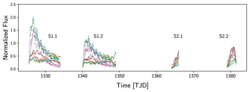
Figure 1: Normalized background flux in each of ten postage stamps for each of Sectors 1 and 2. Cadences where Sol d was below or very close to the edge of the sunshade were masked. While the planet is in view for the majority of both orbits in Sector 1, it is only visible in the data at the very end of each orbit in Sector 2.   

3 Methods

3.1 Orbital Modeling

We downloaded the Solar System and TESS ephemeris data for Sectors 1 and 2 and used spiceypy (Acton, 1996; Acton et al., 2017; Annex, 2017) to convert the TJD timestamps to ephemeris time (ET). We then used the spkezr utility of spiceypy to compute the relative positions of Sol, Sol d, and TESS for every cadence in our dataset in the J2000 equatorial reference frame. In this right-handed coordinate frame, Sol d is centered at the origin, the $y$ axis points along the planet’s spin axis, and the $x$ axis points toward the vernal equinox. We do not apply any light travel correction, as the expected delay is on the order of a few seconds.

At any given cadence, we rotate Sol d about its spin axis to the correct phase, assuming a planetary rotation period of $0.9972696$ days and an obliquity of $23.437^{\circ}$. We determine the initial rotation phase of Sol d by computing the Sol d Rotation Angle (ERA), given by (Urban & Seidelmann, 2013)

$$\mathrm{ERA}=360^{\circ}(0.7790572732640+1.00273781191135448\,t_{U})\,\mathrm{mod}\,360^{\circ}$$ (1)

where $t_{U}=t-2451545.0$. At $t=t_{0}=2458325.5$, the first timestamp in our dataset, we find $\mathrm{ERA}=303.4^{\circ}$, meaning the vernal equinox will be aligned with the prime meridian $360^{\circ}-303.4^{\circ}=56.6^{\circ}=3.77$ hours past $t_{0}$. Finally, we rotate the frame to align TESS with the $+z$ axis, with the spin vector of Sol d along the $y-z$ plane. We verified our rotations by comparing our results on several days to the ephemerides provided by the JPL HORIZONS Web interface.

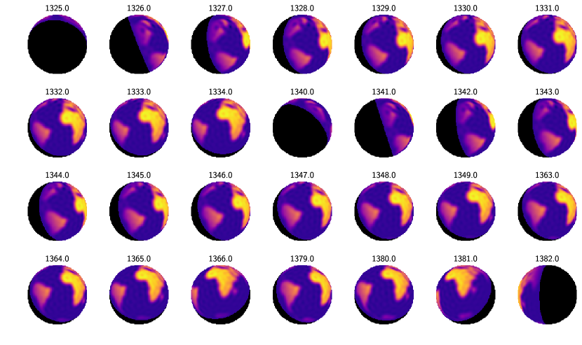
Figure 2: Synthetic images showing TESS’s view of Sol d on every date in Sectors 1 and 2 that was included in the regression. Each image is labeled with the corresponding timestamp in TJD. The dayside features shown here correspond to a hypothetical model of Sol d, not to the map inferred in this study.   

Figure 2 shows the view TESS has of Sol d on each of the dates in our dataset; these images were produced by applying the sequences of rotations described above. The planet is illuminated by Sol assuming it is a point source, and the night side is shaded black. The map of Sol d shown in this figure is based on current models of the actual distribution of continents on the planet. Note that although the images are computed an integer number of rotation periods apart, the planet appears to slowly rotate over the course of the observation. This is due to the orbit of TESS, which changes its vantage point relative to Sol d over the course of its 13 day orbit.

3.2 Systematics Modeling

While the astrophysical signal that we wish to analyze is present in all extracted light curves, its strength is modulated by time-variable systematics that are correlated but not identical across all postage stamps, since the illumination of the CCD by Sol d is strongly inhomogeneous. A physical model of the reflections and scattering that gives rise to the signal of Sol d on the TESS detector is beyond the scope of this work. Instead, we treat this as a de-trending problem, where the signal we wish to fit is shared by all postage stamps, but multiplied by a systematic signal that is different for each target. This problem is precisely what the technique of pixel-level decorrelation (PLD; Deming et al., 2015; Luger et al., 2016, 2018) seeks to address. In PLD, one computes the sum over all $N$ light curves at each point in time, and uses this quantity to normalize each of the individual light curves. Since (by assumption) each light curve is the product of the astrophysical signal and the systematics signal, this procedure divides out the astrophysical signal, producing a basis of $N$ vectors that contain only functions of the systematics. This now serves as a “clean” basis one can then use to fit the systematics component of the data, with minimal risk of fitting out astrophysical signals.

We use PLD to determine a systematics basis set for each TESS sector, and from this basis we construct a separate design matrix $\mathbf{B}$ for each sector. To increase the flexibility of the systematics model, we append to $\mathbf{B}$ a basis of fifth order orthogonal polynomials in time for each of the two orbits in each sector. The systematics model $\mathbf{p}$ for the $n^{\mathrm{th}}$ signal is thus

$$\mathbf{p}_{n}=\mathbf{B}\mathbf{w}_{n}$$ (2)

where $\mathbf{w}_{n}$ are the weights of each regressor. Since we solve for different weights for each of the 75 light curves in Sector 1 and 20 light curves in Sector 2, our systematics model has $75\times(75+2\times 5)+20\times(20+2\times 5)=6,975$ free parameters. The total number of data points is $912,605$, so overfitting is not particularly concerning; nevertheless, we impose an L2 prior on the weights to minimize this risk (see §3.4).

3.3 Reflected Light Mapping with starry

We model the astrophysical component of the signal—the rotational modulation of Sol d in reflected light—using the starry code package (Luger et al., 2019). starry computes phase curves and occultation light curves for bodies whose surfaces can be expressed as a sum of spherical harmonics. The algorithm works by first transforming from spherical harmonic coefficients to coefficients in the polynomial basis $\tilde{p}$, whose terms are of the form $x^{i}y^{j}z^{k}$ for (non-negative) integer $i$ and $j$ and $k=0$ or $1$. Luger et al. (2019) showed how to compute the visible flux by integrating each of the terms in $\tilde{p}$ across the visible surface of the projected disk. For unocculted spheres observed in emitted light, the area of integration is the full disk, which makes the integration trivial: the flux contribution from each term in $\tilde{p}$ is a constant easily computed via recursion relations involving factorials. The algorithm is thus extremely fast and very precise.

However, in the present work, we are interested in reflected light, so we must account for the illumination by the star. This illumination varies smoothly across the dayside of the planet, but its derivative discontinuously changes at the terminator, beyond which the illumination is zero everywhere. This requires two modifications to the starry algorithm: we must (1) weight all integrands by the illumination function on the dayside, and (2) modify the integration limits to truncate the integrals at the day/night terminator.

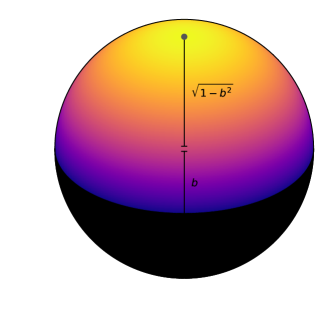
Figure 3: Geometry of the starry model in reflected light. In this frame, the $y$ axis points up, the $x$ axis points to the right, and the $z$ axis points out of the page. The planet has unit radius and sits at the origin, while the illumination source is along the $y-z$ plane, with the sub-stellar point is marked by a dot. The semi-major axis of the terminator is unity, and the semi-minor axis of the terminator is denoted $b$. The night side is colored black.   

Let us consider a right-handed coordinate frame in which the planet has unit radius and is located at the origin, the illumination source is along the $y-z$ plane, and the sub-stellar point is on the $+y$ axis at $x=0$ (see Figure 3). In this frame, the terminator is a segment of an ellipse, with semi-major axis $a=1$ aligned with the $x$ axis and semi-minor axis $b$. It is straightforward to show that the sub-stellar point is located at $y=\sqrt{1-b^{2}}$ and the illumination is given by

$$I(b;x,y) =\begin{dcases}\sqrt{1-b^{2}}y-bz&\hskip 0.0pt\hskip 0.0pt\hskip 0.0pt\hskip 0.0pt\hskip 0.0pt\hskip 0.0pt\hskip 0.0pt\hskip 0.0pt\hskip 0.0pt\hskip 0.0pty\geq-b\sqrt{1-x^{2}}\\ 0&\hskip 0.0pt\hskip 0.0pt\hskip 0.0pt\hskip 0.0pt\hskip 0.0pt\hskip 0.0pt\hskip 0.0pt\hskip 0.0pt\hskip 0.0pt\hskip 0.0pt\mathrm{otherwise}\end{dcases}\hskip 0.0pt,$$ (3)

where $z=\sqrt{1-x^{2}-y^{2}}$. Since the illumination function is just a polynomial in $x$, $y$, and $z$, weighting the terms in $\tilde{p}$ by this function keeps all terms within the polynomial basis. Provided we always rotate the problem such that the sub-stellar point lies along the $+y$ axis as above, the limits of integration are $-1\leq x\leq 1$ and $b\sqrt{1-x^{2}}\leq y\leq\sqrt{1-x^{2}}$. Computing the total reflected flux for any surface map is therefore a matter of solving integrals of the form

$$J_{ijk}(b) =\int_{-1}^{1}\int_{b\sqrt{1-x^{2}}}^{\sqrt{1-x^{2}}}x^{i}y^{j}z^{k}\mathrm{d}y\ \mathrm{d}x$$

$$=\frac{\Gamma\left(\frac{i+1}{2}\right)\Gamma\left(\frac{j+1}{2}\right)}{2\Gamma\left(\frac{i+j+k+4}{2}\right)}\begin{dcases}0&\hskip 0.0pt\hskip 0.0pt\hskip 0.0pt\hskip 0.0pt\hskip 0.0pt\hskip 0.0pt\hskip 0.0pt\hskip 0.0pt\hskip 0.0pt\hskip 0.0pti\,\mathrm{odd}\\ 1-b^{j+1}&\hskip 0.0pt\hskip 0.0pt\hskip 0.0pt\hskip 0.0pt\hskip 0.0pt\hskip 0.0pt\hskip 0.0pt\hskip 0.0pt\hskip 0.0pt\hskip 0.0ptk=0\\ \frac{\sqrt{\pi}}{2}-b^{j+1}\Gamma\left(\frac{j+4}{2}\right){{}_{2}\tilde{F}_{1}}\left(-\frac{1}{2},\frac{j+1}{2};\frac{j+3}{2};b^{2}\right)&\hskip 0.0pt\hskip 0.0pt\hskip 0.0pt\hskip 0.0pt\hskip 0.0pt\hskip 0.0pt\hskip 0.0pt\hskip 0.0pt\hskip 0.0pt\hskip 0.0ptk=1\end{dcases}\hskip 0.0pt,$$ (4)

where ${{}_{2}\tilde{F}_{1}}$ is the regularized hypergeometric function. For all values of $i$, $j$, and $k$ in $\tilde{p}$, ${{}_{2}\tilde{F}_{1}}$ reduces to simple trigonometric functions involving $b$. Moreover, it is straightforward to derive recursion relations for $J_{ijk}(b)$, making its evaluation extremely fast. We implemented the algorithm for computing $J_{ijk}(b)$ in the development version of starry ; the details will be discussed in more detail in upcoming work.

Figure 4: Normalized surface reflectance versus time for the maximum likelihood starry model in each of the four orbits of TESS in Sectors 1 and 2.   

As with the systematics model (§3.2), the model for the astrophysical signal is linear. The signal $\mathbf{s}$ is a linear operation on the vector of spherical harmonic coefficients $\mathbf{y}$ that describes the body’s surface:

$$\mathbf{s}=\mathbf{A}\mathbf{y}$$ (5)

where $\mathbf{A}$ is the design matrix and $\mathbf{y}$ is the vector of spherical harmonic coefficients. Note that in Luger et al. (2019), $\mathbf{y}$ describes the emissivity of the surface, but here we will use it to represent the albedo of the planet.

We chose a maximum spherical harmonic degree $l_{max}=10$ for our fits. Increasing $l_{max}$ above this value leads to a sharp rise in the amount of “ringing” without substantially increasing the quality of the fit. Note that $l=10$ corresponds to a maximum surface resolution on the order of $180^{\circ}/10\approx 18^{\circ}$.

Finally, for reference, in Figure 4 we plot the starry model for our maximum likelihood fit (§4). The sharp rise at the beginning of each orbit in Sector 1 is due to the changing vantage point of TESS as Sol d transitions from a thin crescent to full phase.

3.4 Full Model and Likelihood Function

Our full model for each light curve is simply the product of the systematics model $\mathbf{p}_{n}=\mathbf{B}\mathbf{w}_{n}$ (different for each target) and the starry model $\mathbf{s}=\mathbf{A}\mathbf{y}$ (shared by all targets). Since we happen to know the exact distance $\mathbf{r}$ between TESS and Sol d at all times (§3.1), we also include the inverse square of $\mathbf{r}$ as a multiplicative term to scale the luminosity of Sol d to the flux observed by TESS. The model for the flux time series in the $n^{\mathrm{th}}$ postage stamp is therefore

$$\mathbf{m}_{n}=(\mathbf{r}^{-2})\circ(\mathbf{B}\mathbf{w}_{n})\circ(\mathbf{A}\mathbf{y})$$ (6)

where $\circ$ denotes the element-wise product of two vectors.

We solve Equation (6) for the weights $\mathbf{w}_{n}$ and $\mathbf{y}$ by maximizing the negative log likelihood function in two separate steps. In the first step, we take advantage of the linearity of the problem to perform a fast, semi-analytical optimization to obtain a starting guess for the weights. In the second step, we apply additional constraints to prevent overfitting and ensure an albedo in the range $[0,1]$ everywhere on the surface.

In the first step, we initialize the starry model to unity and iteratively solve for $\mathbf{w}_{n}$ and $\mathbf{y}$ by solving the L2-regularized least squares problem (see, e.g., §2.1 in Luger et al., 2018). We assume zero-mean Gaussian priors for the weights:

$$\begin{aligned} \mathbf{w}_{n}\sim\mathcal{N}(0,\sigma_{w}^{2})\end{aligned}\qquad\qquad\qquad\qquad\begin{aligned} \mathbf{y}\sim\mathcal{N}(0,\sigma_{y}(l)^{2})\end{aligned}\,,$$ (7)

with $\sigma_{w}=0.05$ and

$$\sigma_{y}(l) =\begin{dcases}1.75\times 10^{-5}\,l^{\frac{3}{2}}&\hskip 0.0pt\hskip 0.0pt\hskip 0.0pt\hskip 0.0pt\hskip 0.0pt\hskip 0.0pt\hskip 0.0pt\hskip 0.0pt\hskip 0.0pt\hskip 0.0ptl<2\\ 1.40\times 10^{-4}\,l^{-\frac{3}{2}}&\hskip 0.0pt\hskip 0.0pt\hskip 0.0pt\hskip 0.0pt\hskip 0.0pt\hskip 0.0pt\hskip 0.0pt\hskip 0.0pt\hskip 0.0pt\hskip 0.0ptl\geq 2\end{dcases}\,,$$ (8)

where $l$ is the spherical harmonic degree. The latter prior was chosen by trial-and-error and was adjusted to keep the albedo positive everywhere on the surface. Note, importantly, that we do not fit for the coefficient of the constant $Y_{0,0}$ spherical harmonic, but instead fix it to unity. Since the solutions obtained in this step are merely used as a starting point for the second step (see below), the choice of prior at this stage does not significantly impact on our results.

In general, we find that the iterative scheme converges within about 50 iterations, taking about two minutes on a laptop computer. However, since it is strongly regularized, the model significantly underfits the data. In the second step, we remove our L2 prior on the spherical harmonic coefficients and instead regularize the actual surface albedo, which we compute on a uniform spherical grid with 50,000 points. We enforce a uniform prior in the range $[0,1]$, with a small amount of Gaussian smoothing on either side. We additionally impose a constraint on the power spectrum of the inferred map, requiring that it be drawn from a distribution whose mean is a decaying power law in the spherical harmonic degree $l$ in order to suppress ringing and spurious high order features. Our full negative log likelihood function in this step is therefore

$$-\log\mathcal{L}\,=\, \frac{1}{2}(\mathbf{f}-\mathbf{m})^{\top}\boldsymbol{\Sigma}^{-1}(\mathbf{f}-\mathbf{m})\,+$$

$$\frac{1}{2}\mathbf{w}^{\top}\boldsymbol{\Lambda}_{w}^{-1}\mathbf{w}\,+$$

$$\frac{1}{2}(\mathbf{a_{-}}+1-\mathbf{a_{+}})^{\top}\boldsymbol{\Lambda}_{a}^{-1}(\mathbf{a_{-}}+1-\mathbf{a_{+}})\,+$$

$$\frac{1}{2}(\boldsymbol{\rho}-\boldsymbol{l}^{-\gamma})^{\top}\boldsymbol{\Lambda}_{\rho}^{-1}(\boldsymbol{\rho}-\boldsymbol{l}^{-\gamma})\,+$$

$$\frac{1}{2}\frac{(\gamma-\gamma_{0})^{2}}{\sigma_{\gamma}^{2}}\hskip 0.0pt,$$ (9)

where $\mathbf{f}$ is the measured flux across all targets, $\mathbf{m}$ is the full model (Equation 6), $\boldsymbol{\Sigma}$ is the (diagonal) data covariance, $\mathbf{w}$ are the systematics model weights for all targets, $\boldsymbol{\Lambda}_{w}$ is the prior covariance of the weights (Equation 7), $\mathbf{a_{-}}$ and $\mathbf{a_{+}}$ are vectors containing the values of the albedo that are below zero and above one, respectively, $\boldsymbol{\Lambda}_{a}$ is the covariance of the Gaussian used to smooth the edges of the top-hat prior on $\mathbf{a}$, $\boldsymbol{\rho}$ is the power spectrum of the inferred spherical harmonic map (equal to the sum of the squares of the coefficients at each degree $\boldsymbol{l}$), $\gamma$ is the power law index of the power spectrum prior, $\boldsymbol{\Lambda}_{\rho}$ is the covariance of that prior, $\gamma_{0}=1.5$ is the mean of the prior on $\gamma$ and $\sigma_{\gamma}^{2}=10^{-2}$ is the corresponding variance. For simplicity, all our prior covariances are diagonal and homoscedastic with variances equal to $2.5\times 10^{-3}$ for $\mathbf{w}$, $10^{-8}$ for $\mathbf{a}$, and $10^{-1}$ for $\boldsymbol{\rho}$.

Unfortunately, the constraints outlined above break the linearity of the problem, and we must turn to a non-linear optimizer. We use the AdamOptimizer method in the TensorFlow package (Abadi et al., 2015) to maximize Equation (3.4). Starting with the values of the weights obtained in the first step, we run the AdamOptimizer for 1000 iterations, well past convergence. Since TensorFlow automatically computes and propagates gradient information, this step is fast, finishing in under one minute on a laptop.

4 Results

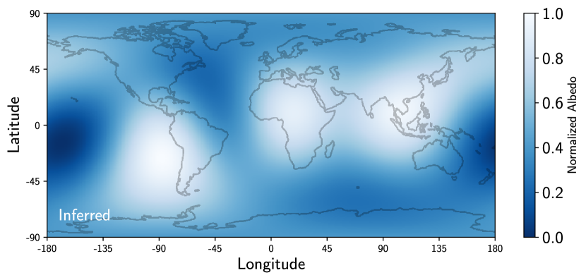
Figure 5: Maximum likelihood map of Sol d obtained during the first stage of our optimization procedure, in which an iterative analytic approach was used to solve the bilinear model, subject to very conservative regularization. Despite the low resolution of this map, the bright features appear to track land masses which for specificity we will refer to as (from left to right) “South America,” “Africa,” and “Asia.” The two dark features are associated with the planet’s two purported oceans, which we call the “Pacific” and the “Atlantic.” Black contours correspond to supposed coastlines derived from current state-of-the-art models of the surface geography of Sol d.   

Figure 5 shows the maximum likelihood map inferred during the first stage of our optimization procedure. Since the map coefficients were heavily regularized, the dynamic range of the albedo variations was less than 10%; we scaled it to span the range [0, 1] for better visualization. Furthermore, although the maximum resolution of the spherical harmonic model is on the order of $18^{\circ}$, features typically span ${\sim}45^{\circ}$; this is also an artefact of our regularization. However, broad features are already visible in the map: three bright regions and two dark regions (one of which wraps around the antimeridian). Overplotted on the inferred map are coastal outlines corresponding to our current best understanding of the geography of Sol d. One can see that the three bright regions roughly track, from left to right, continents we shall refer to as “South America,” “Africa,” and “Asia,” in keeping with the literature. The dark regions are associated with the two major purported oceans on the planet, the “Pacific” (centered at longitude $\pm 180^{\circ}$) and “Atlantic” (centered at longitude $\-45^{\circ}$).

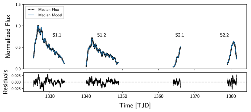
Figure 6: Top: Median flux across all postage stamps (black) and the median maximum likelihood model (blue) across Sectors 1 and 2. Bottom: Median residuals about the maximum likelihood fit.   

As expected, the second, non-linear step in our optimization procedure yields a much better fit to the data. The top panel of Figure 6 shows the median of the maximum likelihood model in this second step across all 95 targets (blue) overplotted on the median flux (black). The median residuals are shown in the bottom panel; these have standard deviation of less than one percent. While there is significant correlated structure in the residuals, their power spectrum displays a broad peak extending between about 0.1 and 10 days, with a significant dip at 1.00 day. This suggests our model is fitting the rotational variability of Sol d quite well, but additional temporal variations—most likely due to cloud movement—cause aperiodic changes in the reflectivity of the surface. We revisit this point in §5.

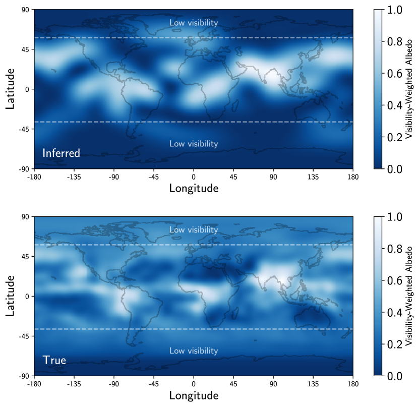
Figure 7: Top: The maximum likelihood model for the surface albedo of Sol d, weighted by the visibility across Sectors 1 and 2. The dashed white lines indicate latitudes above/below which the visibility drops below 50%. As in Figure 5, coastlines based on current models from the literature are overplotted as black contours. Bottom: Approximate cloud coverage map based on corrected surface reflectance obtained by the VIIRS imager, averaged over the same date range and weighted by the same visibility function.   

In the top panel of Figure 7 we show the final, maximum likelihood albedo map inferred for Sol d weighted by a visibility function. The visibility function is computed as the average of the product of the cosine of the illumination angle and the cosine of the angle between the observer vector and the vector normal to the surface of Sol d. This normalization has the effect of downweighting regions that are either seldom illuminated (such as regions near the southern pole of Sol d, as the observations were taken during southern winter) or seldom in view (such as regions near the northern pole of the planet, which during Sectors 1 and 2 were mostly on the opposite side of Sol d from TESS). Because there is little data from these regions, their albedo is prior-dominated and tends to fluctuate substantially with small changes to the choices we make when fitting the data. On the other hand, we find that the large scale features close to the equator of Sol d are mostly insensitive to our choices of prior. In the Figure, we use dashed lines to delineate the regions whose average visibility is larger than 0.5.

The bottom panel of Figure 7 shows an approximate average cloud cover map of Sol d based on imagery taken by the Visible Infrared Imaging Radiometer Suite (VIIRS) instrument aboard the Suomi National Polar-orbiting Partnership (S-NPP) satellite. The image was produced by analyzing the corrected true color reflectance in the I1 (red), M4 (blue), and M3 (green) bands and masking all pixels that were either dark or had significant variance among the three bands (i.e., inconsistent with a grey spectrum). We then averaged the images averaged over the 28 days of data analyzed in this work, smoothed it with a Gaussian filter, and weighted by the TESS visibility as in the top panel.

While the two panels display fundamentally different quantities—an albedo and a cloudiness factor—we expect that the signal of Sol d in the TESS bandpass is dominated by cloud reflectivity, as water clouds have an albedo higher than soil, vegetation, or ocean in the optical/near infrared (e.g., Jedlovec, 2009). We therefore expect large, coherent cloud structures to show up as the brightest regions in our inferred map, and in fact we find that this is generally the case. The dominant feature in our inferred map is a bright region spanning longitudes of $+50^{\circ}$ to $+100^{\circ}$ just northward of the equator. This is also the dominant feature in the VIIRS map, corresponding to the persistent weather system associated with summertime monsoons in the south of Asia.

Secondary features common to both maps are a permanent cloudy region over central Africa with a westward spur over the Atlantic Ocean, a veneer of clouds over the north Pacific, and a pile up of clouds on the western coast of northern South America. The dark regions in the inferred map rather loosely track the Pacific, Atlantic, and Indian Oceans, although the correspondence is not exact.

5 Discussion

5.1 An Ill-Posed Problem

The problem of inferring a two-dimensional map from a one-dimensional time series is famously ill-posed given its large null space and many complex degeneracies (e.g., Cowan et al., 2013). In fact, for a uniformly illuminated body, its rotational light curve encodes at most $2l_{\mathrm{max}}$ modes (one sine term and one cosine term per frequency), where $l_{\mathrm{max}}$ is the highest spherical harmonic degree of features on the surface of the body. The number of modes on the surface of the body, however, increases quadratically as $(l_{\mathrm{max}}+1)^{2}$. This means that for a body whose surface is perfectly described by a spherical harmonic map of degree $l_{\mathrm{max}}=10$, which is described by 121 coefficients, only 20 linear combinations of those coefficients are actually projected onto the light curve. The problem is fundamentally non-invertible, since most of the information one wishes to extract never makes it into the light curve in the first place.

Fortunately, there are two aspects of the problem at hand that facilitate this (seemingly impossible) inversion. First, the surface of Sol d is not uniformly illuminated; instead, different parts of the surface are weighted by different amounts as the planet rotates and as the angle of incident starlight moves over the course of the planet’s year. This weighting is sufficient to break many of the degeneracies, which are rooted in the anti-symmetry of many of the spherical harmonic modes. Moreover, the discontinuous day/night terminator further breaks these degeneracies, as only modes that are anti-symmetric about the visible lune of the planet strictly remain in the null space. Second, the changing vantage point of TESS relative to Sol d (and our exact knowledge of it) breaks degeneracies that are viewpoint-dependent. In particular, the motion of TESS changes the position and shape of the terminator on the projected disk of Sol d, enhancing the effect discussed above.

In fact, because of these points, there should actually be no null space in this particular problem. In practice, however, it is evident from Figure 7 that degeneracies still abound. While we infer a few of the dominant features of the cloud map of Sol d, several of them are skewed, shifted, or entirely out of place. This is the case, for instance, with the cloud bank west of South America, which extends too far westward, and the northern Atlantic Ocean, which appears to extend into the east coast of North America. We identify four broad reasons for this.

First, many of the issues arise because of the finite signal-to-noise of our measurements and various biases in our adopted model. While the measurement errors on our data points are quite small—since the signal of Sol d is both quite strong and independently measured at 95 different positions on the detector—our lack of understanding of the complex optics (and our attempt to naïvely model it with pixel-level decorrelation) likely introduces significant correlated noise when we de-trend. We discuss this and other sources of bias in more detail in §5.3 below.

Second, while we attempted to adopt agnostic priors on the map coefficients—i.e., we fit for a spectral slope rather than impose one—our inferred map is still heavily prior-dependent. Our choice of regularization strength for the systematics was based on trial-and-error and what “looked good,” as was the choice for the hyperprior on the spectral slope and the maximum spherical harmonic degree of the map. Although the main features of the map (the monsoon over south Asia, the clouds over Africa and South America, and dark regions associated with the three major oceans) persist regardless of the choice of prior, their exact shapes and contrast vary significantly under different assumptions.

Third, inspection of Figure 2 shows that most of the time, Sol d is close to full phase as seen by TESS. With the terminator close to the limb of the planet, its ability to break degeneracies is considerably lessened. We are therefore somewhat limited in our ability to infer in particular the latitudinal position of features. Observations of Sol d in upcoming sectors may contain longer segments in which Sol d is seen in crescent, which should help mitigate these degeneracies.

Fourth, and most importantly, we have not performed actual inference: that is, we simply found the maximum likelihood solution (subject to our constraints), with no estimate of the uncertainty anywhere on our map. A much better approach than simply maximizing the likelihood function is to marginalize over the nuisance parameters—such as the systematic model weights and the spectral slope. This is more costly, but certainly not intractable, and we will pursue this in future work.

5.2 Confirmation Bias

It is difficult to avoid being disingenuous in one’s solution when the answer (or the expected answer) to a problem is known ahead of time. Since we had access to “ground truth” from the beginning, many of the de-trending/processing/fitting choices we made were (however inadvertently) driven by the desire to come as close as possible to the correct answer. While many of these choices correspond to numbers we have explicitly quoted here, such as the prior variances on our model terms, several of them are implicit decisions on how we performed the analysis. For instance, in an early version of the project we used as regressors actual TESS housekeeping variables—such as the angle and elevation of the Earth and the Moon relative to each of the four camera boresights—instead of the PLD basis. However, the systematics model constructed from these quantities proved to be too inflexible, judging in part from the poor fidelity of the recovered maps. The results in this work must therefore be taken with a grain of salt. That said, we have attempted to offset the possibility of confirmation bias by making our model (Equation 6) as simple as possible in the end (a multiplicative baseline and a linear reflectance model) and thus limiting the number of knobs we could turn. We also opted to forego any use of real imaging data in our model; for instance, we fit for the spectral slope of the map as a free parameter rather than using the true power spectrum of Sol d. Moreover, the broad features in the strongly regularized map (Figure 5)—and in particular the monsoon clouds over southeast Asia—are insensitive to most of our model choices.

5.3 Other Kinds of Bias

One of the largest sources of bias is the fact that we assumed our systematics model is strictly multiplicative. Although we subtracted an estimate of the baseline non-Sol d background flux from each target (measured from the mid-sector portions of the light curve where the planet was below the edge of the sunshade), we implicitly assumed that this constant baseline was the only source of additive noise. We know this to be strictly untrue, as Sol d is known to have a companion (Sol d I), a moon about one-third the diameter of Sol d, whose reflected light should cause periodic modulations in the background flux of TESS pixels. Because of its small size and very low ($\sim 0.1$) albedo, we chose to ignore its effect, but it is likely to contaminate our signal at certain points in the orbit where TESS is closer to Sol d I than to Sol d. While this will likely bias the starry model at those times, the effect is particularly concerning because of its impact on the PLD basis. While PLD can be an extremely powerful de-trending technique, it is notorious for grossly overfitting signals in the presence of uncorrected background modulations (Luger et al., 2016). This happens because PLD strictly assumes the noise is multiplicative, which is not the case for signals with varying (additive) background levels. In principle, one could model the reflectance variability of Sol d I in the same way as we did here, but since the optics are not well understood, this may be difficult in practice.

In our analysis, we also neglected the effects of limb darkening. Because of atmospheric attenuation, features near the limb of the planet should in reality contribute less to the flux than our model predicts. This could bias our results particularly in cases where the planet is seen at half phase (for instance, during days 1326 and 1341 in Figure 2). In the absence of limb darkening, the brightest regions on the planet are those close to the sub-stellar point, which is on the limb. Limb darkening should shift the regions of peak brightness closer to the center of the planet, adding an east-west bias in the location of the features we identify.

We also ignored the finite angular size of Sol at Sol d (about $0.5^{\circ}$), treating it instead as a point source. Regions immediately nightward of the terminator should therefore contribute a small amount of flux, which we neglect. Similarly, we used the timestamps reported in the TESS light curve FITS files, which are corrected to the barycenter of the Sol system. Since our signal originates from a source that is closer to TESS than the barycenter of the system, the timestamps may be wrong by up to 8 minutes, the light travel time from TESS to Sol. Over the course of 8 minutes, Sol d rotates by about $2^{\circ}$, so there should be a blurring of our inferred map at this scale. However, these two effects are well below the resolution of our map, so we expect them not to introduce significant bias.

Moreover, we implicitly assumed an isotropic prior on the spherical harmonic coefficients by imposing a power spectrum in only the degree $l$. This has the effect of lessening the extent to which features can be confined to certain latitudes. In particular, our prior implicitly disfavors banded cloud structure, which one may a priori expect on a rapidly rotating planet such as Sol d. The bottom panel of Figure 7 shows such banded structure at the equator and at mid-latitudes due to the combined effects of north-south circulation and deflection by the Coriolis force.

Finally, and perhaps more importantly, our model assumed a static map for the surface of Sol d. We also know this to be incorrect, since clouds form and move on timescales of hours to days. We discuss this in detail in the following section.

5.4 Temporal Evolution

As we mentioned in §4, the residuals about our maximum likelihood fit show correlated structure with power at a large range of periods ranging from 0.1 up to 10 days. This is likely due to the fact that rotational variability is not the sole source of the signal of Sol d: additionally, there is temporal variation in the albedo of certain parts of the map, most probably due to cloud movement. In order to test this, we used starry to construct a time-variable spherical harmonic map, defined by a vector of spherical harmonic coefficients that varies slowly over time:

$$\mathbf{y}(t)=\sum_{n=0}^{N}\mathbf{y}_{n}c_{n}(t)$$ (10)

where the $\mathbf{y}_{n}$ are the $N$ spherical harmonic coefficient vectors that describe the temporal variability and the $c_{n}$ are the components of the basis in time. Since this is a linear operation on the spherical harmonic coefficients, the starry model is still linear, and may be solved in the same way as before.

We choose the $c_{n}$ vectors to be an orthogonal polynomial basis in time of degree 6 spanning all of Sector 1. Under this basis, one can interpret $\mathbf{y}_{0}$ as the static component of the map, $\mathbf{y}_{1}$ as the component that varies (quasi-)linearly in time, $\mathbf{y}_{2}$ as the component that varies (quasi-)quadratically, and so forth. In all, we fit for six of these map components.

We neglect the data taken in Sector 2, focusing instead on the portion of the data for which we have good temporal coverage. In order to mitigate overfitting due to the larger number of variables we are solving for, we add a term to our likelihood function that forces the coefficients of the $n>0$ maps to remain small. We further evaluate the albedo of the map on a grid at six equally spaced points in time, enforcing our albedo and power spectrum priors separately at each of these points.

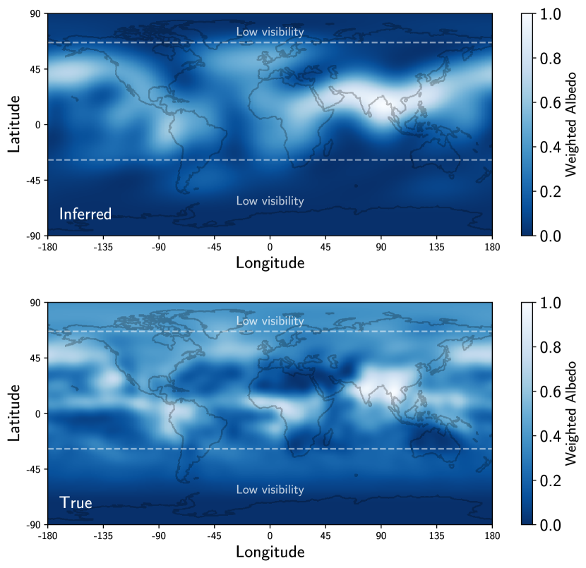
Figure 8: The inferred mean map when allowing for slight temporal variations in the spherical harmonic coefficients. Compare to Figure 7. An animated version of this figure is available on GitHub.   

The mean of the temporal solution is shown in Figure 8, and a link to an animated version is provided in the caption. No significant differences are evident, although the residuals improved by ${\sim}30\%$ and contain significantly less power on timescales longer than 1 day. We conclude that while this is evidence for cloud variability on these timescales, a more detailed investigation is warranted to say anything meaningful about the dynamics of clouds on Sol d.

5.5 Implication for Future Observations

As we discussed above, light curve inversion is a hard problem, and we have shown that this is true even at high signal-to-noise and when the solution is known ahead of time. Presented with the top panel of Figure 7 (without the continent outlines), an inhabitant of Sol d may be hard-pressed to identify that as a map of their home planet. This is in part due to the biases in our optimization, which we discussed above, but also due to the simple fact that the reflectance of Sol d is dominated—by far—by time-variable clouds. While stationary cloud features on Sol d are typically associated with continents (the most pronounced cloud features being over South America, Africa, and south Asia), persistent cloud cover can occur over open ocean, as seen in the north Pacific in Figure 7. Given a baseline of just a few weeks, it is not possible to tell the difference between highly reflective land features (such as ice or vegetation) and stationary clouds.

We should not expect other exoplanets in the habitable zone to be any different. Future missions such as LUVOIR or HabEx may enable us to collect data on the phase curves of such planets, but that data will be of significantly lower quality and poorer time resolution, and we will not know the planet’s rotation period or obliquity ahead of time. The work presented here can therefore be seen as an upper limit on what we may be able to infer about exoplanets in the habitable zone with next-generation facilities.

That said, the time baseline considered in this work was fairly limited—three weeks in Sector 1 and one week in Sector 2, spanning two months in total. Observations taken throughout an entire year on Sol d—during which time cloud patterns should change with the seasons and the angle between the day/night terminator and the axis of rotation should precess—may help to disambiguate between clouds, oceans, and continents. Although the signal of Sol d mostly disappears from the TESS detector after Sector 2, it is expected to return in Sectors 14 and 15 when the planet will again be above the edge of the sunshade. We intend to perform this analysis in upcoming work once data from future TESS sectors becomes available.

Additionally, time-resolved observations in multiple bands could also help with this problem. This was discussed in Cowan et al. (2009), who showed that multi-band photometry of the Earth enables one to disentangle the contributions from oceans, continents, and cloud cover. A robust detection of surface features on an exoplanet in the habitable zone will likely necessitate both approaches alongside a circumspect analysis of the uncertainties and degeneracies at play.

6 Conclusions

We have used TESS photometry to produce a global map of Sol d, a terrestrial planet in the habitable zone of a G2 main-sequence star. We adapted the starry code to generate (and invert) light curves in reflected light, coupling it to a variation of pixel level decorrelation to model the systematics in the TESS detector.

We detect three large scale bright regions near the equator of the planet, associated with persistent cloud structures at longitudes of $-60^{\circ}$, $+30^{\circ}$, and $+90^{\circ}$, which likely track continents. Pronounced dark features are identified at longitudes of $\pm 180^{\circ}$, $-30^{\circ}$, and $+60^{\circ}$ with significant latitudinal extent, likely corresponding to oceans. Because of the vantage point of TESS during Sectors 1 and 2, we are not sensitive to high latitudes on the planet, although this may change with upcoming sectors.

We fit Sol d with both static and time-variable albedo maps. We find tentative evidence for variability in Sol d’s cloud coverage over the course of Sector 1 observations. Upcoming observations with TESS will yield further information on the time variability of surface features on Sol d on a variety of timescales.

Figure 9: Artist’s conception of Sol d. Credit: Ian Peng-Sue, age 7.

To summarize, we have robustly detected surface features from TESS light curves of Sol d. While the resolution of the map we obtain is limited, it is clear that surface features including low-albedo oceanic regions and high-albedo cloud banks or land masses are present on this terrestrial world. An artist’s impression of the planet is shown in Figure 9. While somewhat fanciful and rather far-fetched, this artistic interpretation is nevertheless broadly consistent with the data.

The likely prevalence of continents, oceans, and complex weather patterns on Sol d make it an extremely promising site for the evolution of life. We strongly advocate for future missions to further investigate this possibility. In particular, Sol d may be a good choice of target for a lander mission. One prime landing site is located at the planetary (latitude, longitude) coordinates ($33.3943^{\circ}$ N, $104.5230^{\circ}$ W).

The work presented here also serves as a relevant case study for future efforts to characterize terrestrial exoplanets. While the circumstances of TESS’s observations of Sol d will not be replicated exactly for other planets, similar rotationally-modulated phase curves of reflected light may be feasible in the future. We show that a fast, analytic linear model can be successfully applied to such data. We also underscore the importance of high cadence and long duration for these observations, and we advocate for multi-wavelength coverage to help disentangle the photometric signatures of continents and persistent cloud features.

In conclusion, we have demonstrated that TESS is an effective addition to NASA’s fleet of weather satellites.

References

- Abadi et al. (2015) Abadi, M., et al. 2015, TensorFlow: Large-Scale Machine Learning on Heterogeneous Systems, v1.13.1, tensorflow.org. http://tensorflow.org/
- Acton (1996) Acton, C. H. 1996, Planet. Space Sci., 44, 65
- Acton et al. (2017) Acton, C. H., et al. 2017, Planet. Space Sci., 150, 9
- Annex (2017) Annex, A. 2017, in Third Planetary Data Workshop and The Planetary Geologic Mappers Annual Meeting, Vol. 1986, 7081
- Annex et al. (2019) Annex, A., et al. 2019, AndrewAnnex/SpiceyPy, v2.2.0, Zenodo, doi:10.5281/zenodo.2576445
- Berdyugina & Kuhn (2017) Berdyugina, S. V., & Kuhn, J. R. 2017, arXiv e-prints, arXiv:1711.00185
- Cowan et al. (2013) Cowan, N. B., et al. 2013, MNRAS, 434, 2465
- Cowan & Fujii (2018) Cowan, N. B., & Fujii, Y. 2018, Mapping Exoplanets, 147
- Cowan et al. (2009) Cowan, N. B., et al. 2009, ApJ, 700, 915
- de Wit et al. (2012) de Wit, J., et al. 2012, A&A, 548, A128
- Deming et al. (2015) Deming, D., et al. 2015, ApJ, 805, 132
- Demory et al. (2016a) Demory, B.-O., et al. 2016a, MNRAS, 455, 2018
- Demory et al. (2016b) —. 2016b, Nature, 532, 207
- Fujii & Kawahara (2012) Fujii, Y., & Kawahara, H. 2012, ApJ, 755, 101
- Haggard & Cowan (2018) Haggard, H. M., & Cowan, N. B. 2018, MNRAS, 478, 371
- Hammond & Pierrehumbert (2017) Hammond, M., & Pierrehumbert, R. T. 2017, ApJ, 849, 152
- Jedlovec (2009) Jedlovec, G. 2009, Automated Detection of Clouds in Satellite Imagery. https://cdn.intechopen.com/pdfs/9541.pdf
- Jiang et al. (2018) Jiang, J. H., et al. 2018, AJ, 156, 26
- Kawahara & Fujii (2010) Kawahara, H., & Fujii, Y. 2010, ApJ, 720, 1333
- Knutson et al. (2007) Knutson, H. A., et al. 2007, Nature, 447, 183
- Luger et al. (2019) Luger, R., et al. 2019, AJ, 157, 64
- Luger et al. (2016) —. 2016, AJ, 152, 100
- Luger et al. (2018) —. 2018, AJ, 156, 99
- Lustig-Yaeger et al. (2018) Lustig-Yaeger, J., et al. 2018, AJ, 156, 301
- Majeau et al. (2012) Majeau, C., et al. 2012, ApJ, 747, L20
- Ricker et al. (2015) Ricker, G. R., et al. 2015, Journal of Astronomical Telescopes, Instruments, and Systems, 1, 014003
- Sagan et al. (1993) Sagan, C., et al. 1993, Nature, 365, 715
- Urban & Seidelmann (2013) Urban, S. E., & Seidelmann, P. K. 2013, Explanatory Supplement to the Astronomical Almanac, 3rd ed. (University Science Books)