The radiative corrections to double-Dalitz decays revisited

Abstract:

We revise the radiative corrections to double-Dalitz decays ($P\to\ell\bar{\ell}\ell^{\prime}\bar{\ell}^{\prime}$), completing the full next-to-leading order calculation in QED as compared to existing calculations. As a result, we find mild differences with respect to previous studies, that might be relevant for extracting information about the mesons transition form factors. The latter play an important role in determining the hadronic light-by-light contribution to the anomalous magnetic moment of the muon. Finally, we outline an ongoing extension of this work to the $e^{+}e^{-}\to e^{+}e^{-}P$ processes.

1 Introduction

The transition form factors (TFFs) of pseudoscalar mesons ($P=\pi^{0},\eta,\eta^{\prime}$), commonly denoted as $F_{P\gamma^{*}\gamma^{*}}(q_{1}^{2},q_{2}^{2})$, describe the interaction of the former with two—possibly virtual—photons

$$i\int d^{4}x\ e^{iq_{1}\cdot x}\bra{0}T\{j^{\mu}(x)j^{\nu}(0)\}\ket{P}=\epsilon^{\mu\nu\rho\sigma}q_{1\rho}q_{2\sigma}F_{P\gamma^{*}\gamma^{*}}(q_{1}^{2},q_{2}^{2}).$$ (1)

They have been an object of interest in the past and present years. From one point of view, such an exclusive process with a single—and a priori the simplest—QCD bound state, represents in principle the cleaner one that can be described in pQCD (see Refs. [1, 2] for pioneering works). As such, it serves as a probe of our understanding of QCD dynamics and the pseudoscalar meson structure itself. From a different point of view, and more recently, these have regained interest in connection with their role in the anomalous magnetic moment of the muon, $(g-2)_{\mu}$ [3, 4, 5], which at the moment shows an interesting $3\sigma$ deviation [3] and for which new—more precise results—are expected soon from the new experiment at Fermilab [6] and also, in the future, from J-PARC [7].

A key ingredient here is the description of these form factors at the low energies relevant for $(g-2)_{\mu}$ [5, 8]. While a wealth of experimental data is available in the single-virtual region [i.e. for $F_{P\gamma^{*}\gamma^{*}}(q^{2},0)$] from $e^{+}e^{-}\to e^{+}e^{-}P$ collisions and $P\to\gamma\ell^{+}\ell^{-}$ decays, it is only in the past year that the first doubly-virtual measurement from $e^{+}e^{-}$ colliders for the $\eta^{\prime}$ became available [9]. Still, it would be desirable to gather complementary measurements at lower energies in order to test the most compelling frameworks devised for describing such TFFs in the region relevant to $(g-2)_{\mu}$ [5, 10], and also to compare against the recent lattice results [11]. Experimentally, such a possibility can be brought by the double-Dalitz decays, $P\to\gamma\ell^{+}\ell^{-}\ell^{\prime+}\ell^{\prime-}$, especially for the $\eta$ and $\eta^{\prime}$ cases due to their larger phase space [12, 13, 14, 15, 16, 17, 18]. Notoriously, the required statistics for such measurements would be at hand at the proposed REDTOP facility [21]. Still, an accurate extraction of the TFF would not be possible without a proper implementation of QED radiative corrections. The first calculation of such kind for the double Dalitz decays appeared in [22], that included all diagrams necessary to cancel IR divergencies, but did not represent a full NLO calculation, with some diagrams/topologies missing. In our work [23], we revised such calculation, performing a full NLO evaluation in the soft-photon approximation. As a result, we find corrections to the previous estimate that are likely relevant for the extraction of the doubly-virtual TFF.

2 Full NLO analysis

At LO, the amplitude for double-Dalitz decays $(P\to\ell^{+}\ell^{-}\ell^{\prime+}\ell^{\prime-})$ reads

$$i\mathcal{M}^{LO}=-ie^{4}\frac{F_{P\gamma\gamma}(s_{12},s_{34})}{s_{12}s_{34}}\epsilon_{\mu\nu\rho\sigma}p_{12}^{\mu}p_{34}^{\rho}\left[\bar{u}(p_{1})\gamma^{\nu}v(p_{2})\right]\left[\bar{u}(p_{3})\gamma^{\sigma}v(p_{4})\right],$$ (2)

with an additional exchange contribution ($2\leftrightarrow 3$) whenever identical leptons appear in the final state. For $\ell\neq\ell^{\prime}$, this implies

$$|\mathcal{M}^{LO}|^{2}=\frac{e^{8}|F_{P\gamma\gamma}(s_{12},s_{34})|^{2}}{x_{12}x_{34}}\lambda^{2}\Big{(}2-\lambda_{12}^{2}+y_{12}^{2}-\lambda_{34}^{2}+y_{34}^{2}+(\lambda_{12}^{2}-y_{12}^{2})(\lambda_{34}^{2}-y_{34}^{2})\sin^{2}\phi\Big{)},$$ (3)

where the phase-space variables $\{s_{ij},y_{ij},\phi\}$, and also $\lambda_{(ij)}$, have been defined in [23, 22]. Such result is modified at higher orders in QED. Particularly, denoting the generic amplitude as

$$|\mathcal{M}|^{2}=|\mathcal{M}^{LO}+\mathcal{M}^{NLO}+...|^{2}=|\mathcal{M}^{LO}|^{2}+2\operatorname{Re}\mathcal{M}^{NLO}\mathcal{M}^{LO*}+...=\textrm{LO}+\textrm{NLO},$$ (4)

the NLO contribution to the differential branching ratio stands for the interference of the LO and NLO amplitudes above.

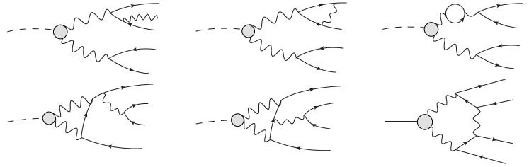
Figure 1: Representatives for each of the NLO contributions. From left to right, up to down: bremsstrahlung, vertex correction (self-energies are implicit), vacuum polarization, three-, four-, and five-point amplitudes.

Representative diagrams contributing to the NLO amplitudes are shown in Fig. 1. Among these diagrams, the vertex, vacuum polarization, and five-point amplitudes, all of them containing IR divergencies, where accounted for already in [22], while the three- and four-point amplitudes where missing. The last types constitute, together with the revision of previous topologies, our main contribution. Further, in order to obtain a finite infrared (IR) result, bremsstrahlung diagrams need to be incorporated as well (see Fig. 1). Employing the soft-photon approximation, these can be expressed as

$$|\mathcal{M}^{BS}|^{2}=-e^{2}|\mathcal{M}^{LO}|^{2}\sum_{i,j}Q_{i}Q_{j}\ I(p_{i},p_{j}),$$ (5)

where $Q_{k}$ and $p_{k}$ stand for the charge and momentum of the $k$-th particle respectively, and $I(p_{i},p_{j})$ are well-known integrals [24] that can be found, adapted to our case of interest, in [23]. In the following, we revise each of the contributions as compared to Ref. [22].

Concerning the vertex corrections, these amount to shifting the $\gamma^{\mu}$ Dirac matrices in Eq. 2 to

$$\gamma^{\mu}\to\gamma^{\mu}F_{1}(q^{2})+\frac{i\sigma^{\mu\lambda}}{2m_{\ell}}q_{\lambda}F_{2}(q^{2})$$ (6)

where $F_{1}(q^{2})$ and $F_{2}(q^{2})$ are the well-known NLO contributions to the Dirac and Pauli form factors. The first one needs to be regularized, together with the self-energies, and contains IR divergencies to be compensated by bremsstrahlung graphs. Its inclusion amounts to a multiplicative factor with respect to the LO result and is in good agreement with Ref. [22]. Concerning the second one, while we agree on the expression for $F_{2}$, we find differences with respect to the resulting matrix element squared. While its impact on the total branching ratio (BR) is negligible [23], it might affect (softly) the differential distributions. Regarding the vacuum polarization, we find good agreement.

Concerning the three- and four-point functions, these have been computed for the first time. In comparison to the vertex functions, these involve an integral over the TFF that, for computational purposes, has been assumed that can be taken as constant or be expressed in a propagator-like form (modulo powers of momenta). Further, for the sake of simplicity, a simple factorized Padé approximant has been employed for numerical results. Analytic expressions for them have been provided, for $\ell\neq\ell^{\prime}$, in [23] in terms of three- and four-point tensor integrals—the full result has been made accessible as ancillary files on arXiv. The three-point topologies deserve further comments since, unlike for the four- and five-point ones, the amplitude itself is divergent for a constant TFF. In our work, two possibilities have been investigated: to use the form factor or to use chiral perturbation theory ($\chi$PT), where a counterterm that is common to $P\to\ell^{+}\ell^{-}$ decays is required to render the amplitude finite. For light pseudoscalars and leptons, the three-point topology is very similar in both approaches, while the performance of $\chi$PT (at this order) deteriorates for heavier pseudoscalars and leptons.

Finally, the five-point topology has been recomputed employing different techniques as compared to Ref. [22], that uses a tensor decomposition of the five-point loop integrals together with spinor amplitudes. In particular, in our final calculations, we compute directly the NLO piece, after summing over polarizations. This allows to decompose the integral in terms of the scalar five-point function and lower-point tensor ones. As a cross-check, we computed the NLO amplitude in terms of five-point tensor integrals that were decomposed into lower-point ones using the method in [25]. Such method overcomes some numerical instabilities encountered in Ref. [22] connected to vanishing Gram determinants, and resulted in identical numerical results as the first method. Since such an integral contains IR divergencies, we also checked that, once combined with bremsstrahlung graphs, the result was IR-finite. Since final expressions are lengthy, it was not possible to compare to the previous results in [22] that might be a source of the mild discrepancies that we found.

3 Numerical results

In the following, we provide results on the correction to the total decay width with a soft-photon cut-off energy $E_{c}$, corresponding to $x_{4\ell}=0.9985$, in analogy to [22]. For the calculation, we employed LoopTools [26, 27] to evaluate the loop integrals that we checked provided the same results as our implementation of the methods in [25]. For the numerical integrals we employed Mathematica’s NIntegrate method as well as the MonteCarlo routines in [28] for each of the contributions, providing compatible results. As a cross-check, the total contribituon of the five-point amplitudes was compatible with $0$ within integration errors, providing an additional cross-check of the correctness of the code [23].

	$\pi^{0}\to 4e$	$K_{L}\to 4e$	$K_{L}\to 2e2\mu$	$K_{L}\to 4\mu$	$\eta\to 4e$	$\eta\to 2e2\mu$	$\eta\to 4\mu$
$\delta(\textrm{NLO})$	$-0.1727(2)$	$-0.2345(1)$	$-0.0842(2)$	$0.0608(2)$	$-0.2409(1)$	$-0.0900(1)$	$0.0455(2)$
$\delta(\textrm{FF})$	$\phantom{-}0.0037(2)$	$\phantom{-}0.0749(2)$	$\phantom{-}0.6942(2)$	$0.8608(3)$	$\phantom{-}0.0207(2)$	$\phantom{-}0.4829(2)$	$0.6202(3)$
no 3,4	$-0.1718(2)$	$-0.2262(2)$	$-0.0767(1)$	$0.0704(1)$	$-0.2301(1)$	$-0.0836(1)$	$0.0535(1)$
Barker	$-0.160(2)$	$-0.218(1)$	$-0.066(1)$	$0.084(1)$	$-$	$-$	$-$
BR(LO+NLO)	$2.840(1)10^{-5}$	$5.120(1)10^{-5}$	$4.436(1)10^{-6}$	$1.851(1)10^{-9}$	$5.202(1)10^{-5}$	$5.393(1)10^{-6}$	$10.289(2)10^{-9}$

Table 1: Numerical results for the radiative corrections (second row). The third shows the effects of including a TFF on the LO result. The fourth row contains the same corrections included in Ref. [22] (in fifth row), that show the disagreement. The last row stands for the BR at NLO accuracy.

The main results for the BR are given in Table 1, that displays the quantity $\delta(NLO)=\textrm{BR}^{NLO}/\textrm{BR}^{LO}-1$, where NLO superscripts refers to the results containing LO and NLO contributions to the BR. The second row, $\delta(\textrm{NLO})$, is our main result, obtained for a non-constant TFF, which effect is outlined in the third row. The fourth includes only those contributions in [22] and a constant TFF, so that it can be readily compared to [22], fifth row.

As advanced, we find some discrepancies—of the order of $1\%$ compared to [22]. The source of this is unclear: a few possibilities have been outlined, but numerics in their MC generator could contribute too. Finally, we note that for heavier pseudoscalars the previously ommitted three- and four-point topologies represent an additional $1\%$ effect—likely relevant for extracting information about the doubly-virtual TFF [17], yet a quantitative statement would require a MC simulation.

4 Connection with $e^{+}e^{-}\to e^{+}e^{-}P$ production

As an extension, this process can be related via crossing symmetry to $e^{+}e^{-}\to e^{+}e^{-}P$ production [29] (see Fig. 2), yet bremsstrahlung diagrams need to be recomputed in the appropriate reference frame—that of $e^{+}e^{-}$. As such, these results can be employed to complement the current NLO calculation in EKHARA 3.0 [30], that misses the three-, four-, and five-point topologies and is a work in progress.

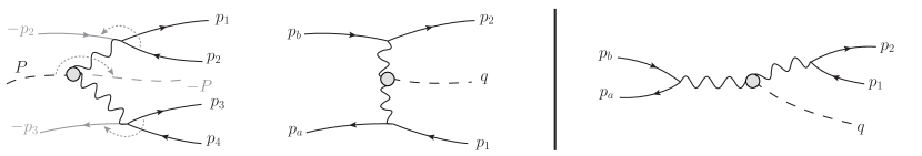
Figure 2: Left block shows the choice for crossing relations from direct double-Dalitz terms (left) to the $e^{+}e^{-}\to e^{+}e^{-}P$ $t$-channel ones (center). The right block is the s-channel contribution to the latter process that would be crossed-related to the double-Dalitz exchange terms.

For completeness, we detail here the required replacements relating both processes via crossing symmetry. With the choice in Fig. 2, the amplitudes referred in [23] as Direct(Exchange) connect to the $t$- and $s$- channels for the mentioned process. Particularly, this is realized at the amplitude level through:

$$p_{1}\to p_{2}, p_{2}\to-p_{b}, p_{3}\to-p_{a}, p_{4}\to p_{1}, P\to-q,$$

$$\bar{u}_{1}\to\bar{u}_{2}, v_{2}\to u_{b}\phantom{-}, \bar{u}_{3}\to\bar{v}_{a}\phantom{-}, v_{4}\to v_{1}.$$ (7)

Defining the following invariants

$$(p_{a}+p_{b})^{2}=s,\ (p_{a}-p_{1})^{2}=t_{1},\ (p_{b}-p_{2})^{2}=t_{2},\ (q+p_{1})^{2}=s_{1},\ (q+p_{2})^{2}=s_{2},$$ (8)

it implies the following connection

$$2p_{12}\cdot p_{34} {}\to 2(p_{a}-p_{1})\cdot(p_{b}-p_{2}) {}=M^{2}-t_{1}-t_{2},$$ (9)

$$2\bar{p}_{12}\cdot p_{34} {}\to -2(p_{2}+p_{b})\cdot(p_{a}-p_{1}) {}=2m^{2}+M^{2}-2s_{2}+t_{1}-t_{2},$$ (10)

$$2\bar{p}_{34}\cdot p_{12} {}\to 2(p_{1}+p_{a})\cdot(p_{b}-p_{2}) {}=-2m^{2}-M^{2}+2s_{1}+t_{1}-t_{2},$$ (11)

$$2\bar{p}_{12}\cdot\bar{p}_{34} {}\to -2(p_{1}+p_{a})\cdot(p_{b}+p_{2}) {}=4m^{2}-M^{2}-4s+2s_{1}+2s_{2}-t_{1}-t_{2},$$ (12)

$$(\epsilon^{p_{1}p_{2}p_{3}p_{4}})^{2} {}\to (\epsilon^{p_{a}p_{b}p_{1}p_{2}})^{2} {}=-\Delta_{4},$$ (13)

where $\Delta_{4}$ is the corresponding $4\times 4$ Gram determinant. This allows to define the crossed-related version of the old variables as

$$M^{4}\lambda^{2} {}\to \bar{\lambda}^{2} {}=(M^{2}-t_{1}-t_{2})^{2}-4t_{1}t_{2},$$ (14)

$$y_{12} {}\to \bar{y}_{12} {}=(2m^{2}+M^{2}-2s_{2}+t_{1}-t_{2})\bar{\lambda}^{-1},$$ (15)

$$y_{34} {}\to \bar{y}_{34} {}=(-2m^{2}-M^{2}+2s_{1}+t_{1}-t_{2})\bar{\lambda}^{-1},$$ (16)

$$\cos{\phi} {}\to \cos{\bar{\phi}} {}=\frac{(M^{2}-t_{1}-t_{2})\bar{y}_{12}\bar{y}_{34}-(4m^{2}-M^{2}-4s+2s_{1}+2s_{2}-t_{1}-t_{2})}{\left[4(t_{2}-4m^{2}-t_{2}\bar{y}_{12})(t_{1}-4m^{2}-t_{1}\bar{y}_{34})\right]^{1/2}},$$ (17)

$$\sin^{2}{\phi} {}\to \sin^{2}{\bar{\phi}} {}=-16^{2}\Delta_{4}\left(4(t_{2}-4m^{2}-t_{2}\bar{y}_{12})(t_{1}-4m^{2}-t_{1}\bar{y}_{34}\right)^{-1}.$$ (18)

Finally, the Bremsstrahlung contribution, with the soft-photon energy in the colliding $e^{+}e^{-}$ frame, reads

$$e^{2}I(p_{i},p_{j})=\frac{\alpha}{\pi}\frac{1+\beta_{ij}^{2}}{4\beta_{ij}}\Bigg{[}2\ln\left(\frac{1+\beta_{ij}}{1-\beta_{ij}}\right)\ln\left(\frac{2E_{c}}{m_{\gamma}}\right)+\frac{1}{4}\ln^{2}\left(\frac{\Omega_{i}^{-}}{\Omega_{i}^{+}}\right)-\frac{1}{4}\ln^{2}\left(\frac{\Omega_{j}^{-}}{\Omega_{j}^{+}}\right)$$

$$+\operatorname{Li}_{2}\left(1-\frac{\Upsilon_{ij}\Omega_{i}^{-}}{\beta_{ij}}\right)+\operatorname{Li}_{2}\left(1-\frac{\Upsilon_{ij}\Omega_{i}^{+}}{\beta_{ij}}\right)-\operatorname{Li}_{2}\left(1-\frac{\Upsilon_{ij}\Omega_{j}^{-}}{\beta_{ij}\alpha_{ij}}\right)-\operatorname{Li}_{2}\left(1-\frac{\Upsilon_{ij}\Omega_{j}^{+}}{\beta_{ij}\alpha_{ij}}\right)\Bigg{]},$$ (19)

with $\beta_{ij}^{2}=1-4m^{2}(p_{i}+p_{j})^{-2}$ and $\alpha_{ij}=(1+\beta_{ij})/(1-\beta_{ij})^{-1}$, $\Upsilon_{ij}=2(\alpha p_{i}^{0}-p_{j}^{0})(p_{i}+p_{j})^{-2}$. The additional parameters are given by

$$(p_{a(b)}+p_{1(2)})^{2} {}=4m^{2}-t_{1(2)}\equiv s_{a1(b2)},$$ (20)

$$(p_{a(b)}+p_{2(1)})^{2} {}=m^{2}+s+t_{2(1)}-s_{1(2)}\equiv s_{a2(b1)},$$ (21)

$$(p_{1}+p_{2})^{2} {}=2m^{2}+M^{2}+s-s_{1}-s_{2},\equiv s_{12}$$ (22)

$$\Omega^{\pm}_{a,b} {}=\sqrt{s}(1\pm\beta)/2,$$ (23)

$$\Omega^{\pm}_{1(2)} {}=\left[s+m^{2}-s_{2(1)}+\lambda^{1/2}(s,s_{2(1)},m^{2})\right](2\sqrt{s})^{-1},$$ (24)

$$\Upsilon_{ab} {}=2\beta(\sqrt{s}(1-\beta))^{-1},$$ (25)

$$\Upsilon_{a2(b1)} {}=\left[s(\alpha_{a2(b1)}-1)+s_{1}-m^{2}\right](s_{a2(b1)}\sqrt{s})^{-1},$$ (26)

$$\Upsilon_{a1(b2)} {}=\left[s(\alpha_{a1(b2)}-1)+s_{2}-m^{2}\right](s_{a1(b2)}\sqrt{s})^{-1},$$ (27)

$$\Upsilon_{12} {}=\left[(s+m^{2})(\alpha_{12}-1)+s_{1}-\alpha_{12}s_{2}\right](s_{12}\sqrt{s})^{-1}.$$ (28)

with $s_{ij}\equiv(p_{i}+p_{j})^{2}$ and $\lambda(a,b,c)\equiv a^{2}+b^{2}+c^{2}-2ab-2ac-2bc$. Finally, for $p_{i}=p_{j}$,

$$e^{2}I(p_{a,b},p_{a,b}) {}=\frac{\alpha}{\pi}\left[\ln\left(\frac{2E_{c}}{m_{\gamma}}\right)+\frac{1}{2\beta}\ln\left(\frac{1-\beta}{1+\beta}\right)\right],$$ (29)

$$e^{2}I(p_{1(2)},p_{1(2)}) {}=\frac{\alpha}{\pi}\left[\ln\left(\frac{2E_{c}}{m_{\gamma}}\right)+\frac{s+m^{2}-s_{2(1)}}{2\lambda^{1/2}(s,s_{2(1)},m^{2})}\ln\left(\frac{\Omega^{-}_{1(2)}}{\Omega^{+}_{1(2)}}\right)\right].$$ (30)

5 Conclusions and Outlook

In this work, we have revisited and completed the full NLO calculation for double-Dalitz pseudoscalar decays in the soft-photon approximation. In doing so, we find small numerical differences with respect to the topologies already accounted for in the existing calculation, the source of which could not be determined precisely. In addition, the new topologies have a small but likely non-negligible effect for the extraction of the doubly-virtual TFF. The results have been provided in a Mathematica notebook available at arXiv as an ancillary file. Also, this work is relevant for completing the NLO corrections for pseudoscalar production at $e^{+}e^{-}$ colliders, which is currently a work in progress.

- [1] G. P. Lepage and S. J. Brodsky, Exclusive Processes in Perturbative Quantum Chromodynamics, Phys. Rev. D22 (1980) 2157.
- [2] G. P. Lepage and S. J. Brodsky, Exclusive Processes in Quantum Chromodynamics: Evolution Equations for Hadronic Wave Functions and the Form-Factors of Mesons, Phys. Lett. 87B (1979) 359.
- [3] F. Jegerlehner and A. Nyffeler, The Muon g-2, Phys. Rept. 477 (2009) 1 [0902.3360].
- [4] T. Blum, ed., Hadronic contributions to the muon anomalous magnetic moment Workshop. : Quo vadis? Workshop. Mini proceedings, 2014.
- [5] P. Masjuan and P. Sanchez-Puertas, Pseudoscalar-pole contribution to the : a rational approach, Phys. Rev. D95 (2017) 054026 [1701.05829].
- [6] Fermilab P989 collaboration, The Fermilab muon (g-2) project, Nucl. Phys. Proc. Suppl. 218 (2011) 237.
- [7] J-PARC g-2 collaboration, New g-2 experiment at J-PARC, Chin. Phys. C34 (2010) 745.
- [8] A. Nyffeler, Precision of a data-driven estimate of hadronic light-by-light scattering in the muon : Pseudoscalar-pole contribution, Phys. Rev. D94 (2016) 053006 [1602.03398].
- [9] BaBar collaboration, Measurement of the transition form factor, Phys. Rev. D98 (2018) 112002 [1808.08038].
- [10] M. Hoferichter, B.-L. Hoid, B. Kubis, S. Leupold and S. P. Schneider, Dispersion relation for hadronic light-by-light scattering: pion pole, JHEP 10 (2018) 141 [1808.04823].
- [11] A. Gérardin, H. B. Meyer and A. Nyffeler, Lattice calculation of the pion transition form factor with Wilson quarks, 1903.09471.
- [12] F. Perrsson, Effects of different form-factors in meson photon photon transitions and the muon anomalous magnetic moment, Master’s thesis, Lund U., Dept. Theor. Phys., 1999.
- [13] C.-C. Lih, Study of pi0 and eta decays containing dilepton, J. Phys. G38 (2011) 065001 [0912.2147].
- [14] T. Petri, Anomalous decays of pseudoscalar mesons, Ph.D. thesis, Julich, Forschungszentrum, 2010. 1010.2378.
- [15] C. Terschlüsen, B. Strandberg, S. Leupold and F. Eichstädt, Reactions with pions and vector mesons in the sector of odd intrinsic parity, Eur. Phys. J. A49 (2013) 116 [1305.1181].
- [16] G. D’Ambrosio, D. Greynat and G. Vulvert, Standard Model and New Physics contributions to and into four leptons, Eur. Phys. J. C73 (2013) 2678 [1309.5736].
- [17] R. Escribano and S. Gonzàlez-Solís, A data-driven approach to and single and double Dalitz decays, Chin. Phys. C42 (2018) 023109 [1511.04916].
- [18] E. Weil, G. Eichmann, C. S. Fischer and R. Williams, Electromagnetic decays of the neutral pion, Phys. Rev. D96 (2017) 014021 [1704.06046].
- [19] BESIII collaboration, The two-photon physics program at BESIII, Nucl. Part. Phys. Proc. 287-288 (2017) 99.
- [20] BESIII collaboration, The Physics Program at BESIII, EPJ Web Conf. 166 (2018) 00017.
- [21] REDTOP collaboration, The REDTOP project: Rare Eta Decays with a TPC for Optical Photons, PoS ICHEP2016 (2016) 812.
- [22] A. R. Barker, H. Huang, P. A. Toale and J. Engle, Radiative corrections to double Dalitz decays: Effects on invariant mass distributions and angular correlations, Phys. Rev. D67 (2003) 033008 [hep-ph/0210174].
- [23] K. Kampf, J. Novotný and P. Sanchez-Puertas, Radiative corrections to double-Dalitz decays revisited, Phys. Rev. D97 (2018) 056010 [1801.06067].
- [24] G. ’t Hooft and M. J. G. Veltman, Scalar One Loop Integrals, Nucl. Phys. B153 (1979) 365.
- [25] A. Denner and S. Dittmaier, Reduction of one loop tensor five point integrals, Nucl. Phys. B658 (2003) 175 [hep-ph/0212259].
- [26] T. Hahn and M. Perez-Victoria, Automatized one loop calculations in four-dimensions and D-dimensions, Comput. Phys. Commun. 118 (1999) 153 [hep-ph/9807565].
- [27] T. Hahn and M. Rauch, News from FormCalc and LoopTools, Nucl. Phys. Proc. Suppl. 157 (2006) 236 [hep-ph/0601248].
- [28] T. Hahn, CUBA: A Library for multidimensional numerical integration, Comput. Phys. Commun. 168 (2005) 78 [hep-ph/0404043].
- [29] P. Sanchez-Puertas, K. Kampf and J. Novotný, A revision of radiative corrections to double-Dalitz decays, EPJ Web Conf. 199 (2019) 02014 [1809.01868].
- [30] H. Czyz and P. Kisza, EKHARA 3.0: an update of the EKHARA Monte Carlo event generator, Comput. Phys. Commun. 234 (2019) 245 [1805.07756].
- [31] G. A. Schuler, Two photon physics with GALUGA 2.0, Comput. Phys. Commun. 108 (1998) 279 [hep-ph/9710506].
- [32] H. Czyz and S. Ivashyn, EKHARA: A Monte Carlo generator for e+ e- to e+ e- pi0 and e+ e- to e+ e- pi+ pi- processes, Comput. Phys. Commun. 182 (2011) 1338 [1009.1881].