Limits of density-constrained optimal transport
Abstract
We consider the problem of dynamic optimal transport with a density constraint. We derive variational limits in terms of -convergence for two singular phenomena. First, for densities constrained near a hyperplane we recover the optimal flow through an infinitesimal permeable membrane. Second, for rapidly oscillating periodic constraints we obtain the optimal flow through a homogenized porous medium.
1 Introduction
Over the last few years, optimal transport has become a vibrant research area with many different applications. In particular, density-constrained flow problems have garnered significant interest starting with the seminal work of Ford and Fulkerson [11].
In recent years, the theory of constraints has been adapted to optimal transport, first as a static version in [14] and then as dynamic constraints in [8] and [9].
The model we use is based on the dynamic formulation of the Kantorovich distance due to Benamou and Brenier [3],
| (1) |
Here the infimum is taken over all curves of probability measures with fixed endpoints.
In this paper, we constrain the densities of all intermediate measures by some measurable maximal density . In this article is a manifold with boundary, typically or the torus .
More precisely we consider first the space of finite nonnegative Radon measures on equipped with the weak- (also called narrow) topology in duality with .
By extension the space of weakly- continuous curves of finite nonnegative Radon measures is
| (2) |
We study in this article the constrained transport functional ,
| (3) |
Note that the constraint is closed under weak- convergence by the Portmanteau theorem.
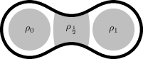
For we recover the classical Benamou-Brenier formula. If then every admissible is absolutely continuous with density almost everywhere. The case for some nonconvex , e.g. an hourglass (see Figure 1), models optimal transport of an incompressible but sprayable fluid. This specific problem was treated in [16], [17]. If is convex, -geodesics between two measures satisfy the density constraints. If is not convex, optimal curves under the constraint are not -geodesics and interact with the constraint.
We find the variational limits of two singular phenomena.
1.1 Thin permeable membranes
The first is the derivation of an infinitesimal membrane from the constraint
| (4) |
for some .
Then, as , we derive an effective variational model in the sense of -convergence as introduced by De Giorgi. We refer to [5] and [10] for comprehensive overviews of the theory.
The limit functional acts on curves of nonnegative Radon measures on the topological disjoint union of the closed half-spaces
and is given by ,
| (5) |
where we use the identification . The infimum is taken over all pairs of distributional solutions to the continuity equations
| (6) |
meaning that in both half-spaces, for all the following equation holds
Here is a vector-valued finite Radon measure which is absolutely continuous with respect to and is the flux through the membrane, with positive sign denoting flux from the lower into the upper half-space.
Theorem 1.1.
Let . Then, as , the energies -converge to the limit functional in the sense that
-
(lower bound)
if in for every , and in for every then
(7) -
(upper bound)
for all curves with there exists a sequence in with in for every , and in for every and
(8)
We prove this theorem in Section 6. Note that the part includes the mass in the membrane, which is locally bounded by .
Since -convergence implies the convergence of minimizers, the associated minimal energies between two measures of equal mass converge as well, as do the minimizing curves themselves.
1.2 Homogenization of periodic constraints
The second result concerns the effective limit as for
| (9) |
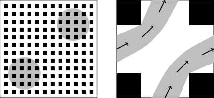
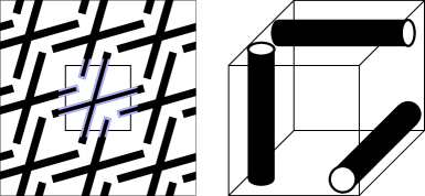
where is -periodic. This problem is related to the periodic homogenization of elliptic functionals, see [6]. In fact it is a special case of -quasiconvex homogenization treated in [7]. In particular it includes perforated domains, where for some periodic open set , modelling the optimal flow of an incompressible fluid through a porous medium (see Figure 2), which has received a lot of attention in recent years, see e.g. [19], [24]. To the best knowledge of the authors this is a new development in the derivation of porous media equations from inhomogenous materials via optimal transport.
We will assume throughout the article that satisfies
-
(A1)
is -periodic.
-
(A2)
is open, connected, and Lipschitz bounded.
-
(A3)
is measurable.
-
(A4)
for some , for almost every .
We note that can be interpreted as either a function on the torus or as a periodic function on . The connectedness of is stronger than connectedness of .
Under these admissibility assumptions, we show -convergence of to the homogenized transport cost ,
| (10) |
where only absolutely continuous curves are allowed. Otherwise is defined to be .
The homogenized energy density is given by
| (11) |
and the infimum is taken among all such that almost everywhere and , and all such that , and .
Theorem 1.2.
Let satisfy the assumptions (A1) - (A4). Then, as , and in for every , -converges to in the sense that
-
(lower bound)
if in for every , then
(12) -
(upper bound)
for all curves with there exists a sequence in with in for every , and
(13)
Remark 1.3.
In the one-dimensional case is given by
| (14) |
where is the mobility. Since is convex (see Lemma 7.1), this means that the mobility must be concave, which signifies a congestion effect.
In Section 2 we prove lower-semicontinuity and compactness of the functionals , and , which is relevant for later sections. In Section 3 we find the dual problems of (3), (5) and (10) and characterize the minimizers by the respective Euler-Lagrange equations. In Section 4 we state the PDE solved by the steepest descent of the Helmholtz free energy functional for each cost. Additionally, in Section 5 we give an example of an optimal curve under a nontrivial density constraint. Finally, in Section 6 and Section 7 we prove Theorem 1.1 and Theorem 1.2 respectively.
2 Compactness
Lemma 2.1.
The functionals , , and defined in (3), (5), and (10) are lower semicontinuous with respect to pointwise weak- convergence on , where is or , , or respectively.
Given a fixed finite Radon measure , all families of curves starting in with bounded energies have a subsequence converging pointwise weak- in .
Proof.
Compactness in the constrained and homogenized case follows from the fact that in (3), (10), the functional is bounded from below by the Wasserstein action (1). For (10), this bound is shown in Lemma 7.1. The compactness then follows from the tightness of balls in Wasserstein space and the uniform continuity of sequences of curves with finite energy.
We show compactness in the membrane case in two steps. First, for define a test function such that , outside of , in , and . Then
| (15) | ||||
The last term is uniformly small in as , showing tightness of the .
Now pick a countable family that is dense in . Then whenever , , we have
| (16) | ||||
It follows that for every . By Helly’s Selection Theorem there exists a subsequence and a curve such that for every and every . By tightness, for every , which proves the compactness.
In cases (3) and (10), to prove the lower bound, take a sequence of curves with finite energy. We see by Hölder’s inequality that
| (17) |
where or , respectively. The right hand side is bounded, so that a subsequence converges vaguely (not necessarily weak- in the case of (5)) to some . We note that is absolutely continuous with respect to , so that by the disintegration theorem for some defined for almost every , and in .
The same argument works in case , yielding finite measures . Additionally, in . The limits then solve in , and by Fubini’s theorem and the weak lower semicontinuity of the norm
| (18) |
To show lower semicontinuity of the remaining term
| (19) |
with , we use Theorem 2.34 in [2], which states that for convex, lower semicontinuous, with recession function , the functional defined on
| (20) |
is vaguely sequentially lower semicontinuous. We apply this to the sequence , which in any case converges vaguely to . The function is either in cases (3) and (5) or in case (10). We now have to do some extra work depending on the case:
In case (3), we have to show that for every open set . This is the Portmanteau theorem, found in e.g. [2, Example 1.63].
In case (10), we know from Lemma 7.1 that is convex and lower semicontinuous. We have to make sure that the singular part of vanishes. Indeed, this holds if , as in that case for every , and this property is inherited by . Moreover, if the energy is finite.
In case (5), we have nothing more to show. This completes the proof. ∎
3 Duality and minimality
In this section, we characterize the dual problems to (3), (5), and (10) and find the Euler-Lagrange equations. To this end, we fix endpoints with finite and equal mass.
3.1 Constrained optimal transport
Here we minimize the action functional
| (21) |
subject to for every open and in , and fixed. We introduce the Lagrange multiplier and write by Sion’s minimax theorem
| (22) | ||||
The last term is the constrained dual problem. Note that wherever , we formally recover the Kantorovich dual.
By the complementary slackness theorem, the minimizer and maximizer are characterized by the Euler-Lagrange equations
| (23) |
Here is the Lagrange multiplier to the constraint on acting as a pressure on the potential.
3.2 Optimal membrane transport
Here we minimize
| (24) |
subject to and in , and fixed. We introduce the Lagrange multipliers and write by Sion’s minimax theorem, denoting ,
| (25) | ||||
The last term is the constrained dual problem. Note that as , we formally recover the Kantorovich dual problem in , whereas as , we formally recover two separate Kantorovich dual problems in .
By the complementary slackness theorem, the minimizers and maximizers are characterized by the Euler-Lagrange equations
| (26) |
3.3 Homogenized optimal transport
Here we minimize
| (27) |
subject to in , and fixed. We introduce the Lagrange multiplier and write by Sion’s minimax theorem
| (28) | ||||
The last term is the dual problem. We check that for on , we have
| (29) |
as expected.
By the complementary slackness theorem, the minimizer and maximizer are characterized by the Euler-Lagrange differential inclusions, which are stated in terms of the partial Legendre transform as
| (30) |
This is a general formulation of congested mean field games. A similar model of congested mean field game is treated in e.g. [4].
To be more specific, in the idealized case , , the mean field game equation is given by
| (31) |
4 Gradient flows
We now look at the formal constrained gradient flows of the functionals
| (32) |
with the Gibbs free energy, and the gas constant and the temperature respectively.
We will write down the PDE corresponding to steepest descent of with costs given by (3), (5), and (10). Without loss generality we assume .
4.1 Constrained gradient flow
Given , we want to find minimizing
| (33) | ||||
subject to on . We introduce a Lagrange multiplier , , , and write the above problem as
| (34) | ||||
We see that the minimizer can be written , where solves the elliptic obstacle problem
| (35) |
Physically, the difference between and the chemical potential acts as a hydrostatic pressure with .
Inserting into the continuity equation yields a constrained version of the Fokker-Planck equation,
| (36) |
Note that in [13], the authors rigorously derive the unconstrained Fokker-Planck equation as the -gradient flow of . We note that this version of the constrained Fokker-Planck equation differs from the Stefan problem treated in e.g. [18], which is not mass-preserving.
4.2 Membrane gradient flow
Here, given , and a Gibbs free energy , we find minimizing
| (37) |
Inserting the minimizers into the continuity equation yields two Fokker-Planck equations coupled through the Teorell equation on the membrane [23],
| (38) |
4.3 Homogenized gradient flow
5 The stark constraint
In the following we give a simple one-dimensional example of an optimal curve under a nontrivial density constraint, which bounds the density by on .
| (41) |
where . We call this the stark constraint. We construct an optimal curve starting in and ending in the uniform density .
We choose this example because the solution breaks conservation of momentum, while kinetic energy is conserved. The calculations in this case are straightforward but already quite lengthy. The complexity only increases in higher dimensions and with more variation in .
We choose the following ansatz for the optimal curve:
| (42) |
We see that any for any Borel , and the boundary conditions are satisifed if and only if and . The momentum field solves the continuity equation
| (43) |
with action given by
| (44) |
where . The minimizer satisfies , where is the unique constant compatible with the boundary conditions and . We see that
| (45) |
and consequently
| (46) |
We claim that is optimal among all curves independent of the ansatz. To see this we consider the dual problem. Let
| (47) |
where and for . Formally, we have
| (48) | ||||
which is half the primal cost . By duality and must be optimal. In fact, they formally solve (23) with pressure
| (49) |
However, at , is not differentiable and at , it is not continuous. To make the optimality precise, we approximate with -functions , with uniformly and in . Then for every , we have
| (50) |
This shows that is optimal. Letting , optimality of follows.
6 The membrane limit
Because -convergence is compatible with partial minimization, the minimum costs for all curves also -converge.
Proof of the lower bound.
Consider a family of curves of bounded nonnegative measures with , where and . Also find the respective minimizing momentum fields such that in and
| (52) |
We shall assume throughout the proof that (52) is bounded by some constant independent of by extracting a subsequence, as without the existence of a bounded energy subsequence there is nothing to prove.
We now employ the standard dimension reduction technique of blowing up the thin constrained region, as was done in e.g. [12]. We introduce the notation . To that end, let be defined by
| (53) |
so that .
We define and , i.e.
| (54) |
By this choice, , and
| (55) |
Because in , it follows that strongly in , and that a subsequence of converges weakly in to some . In addition, in . Thus, the continuity equation holds for the limit, i.e. in , i.e. . By Mazur’s Lemma, it follows that
| (56) | ||||
Dividing both sides by yields the part of the lower bound in the membrane . For the outer part of the membrane we find by Jensen’s inequality
| (57) |
because the energy is finite. Also , from which we infer that a subsequence of converges vaguely to some Radon measure with , where
| (58) |
By Lemma 2.1 () we have
| (59) |
All in all we obtain
| (60) | ||||
We define and . Let and let be an extension of . Then
| (61) | ||||
| (62) | ||||
| (63) | ||||
| (64) |
which shows the continuity equation (6) in the lower half-space. The upper half-space works similarly. ∎
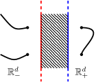
To prove the upper bound, we find it is useful to represent the limit problem in Lagrangian coordinates. For curves in with finite kinetic action, this is done by the well-known superposition principle due to Smirnov [22] and applied to optimal transport in e.g. [1]. Here, the particle trajectories may jump between the half-spaces and are thus not continuous. A natural class of curves are the special curves of bounded variation defined below, see also Figure 3.
Definition 6.1.
Given , we define the class of curves in containing all such that is absolutely continuous up to a finite jump set , with velocity , and mirrored traces at the jumps for all , where is the mirror function mapping to .
We also define the subclass as all curves with jump traces on the boundary .
We equip with the notion of weak convergence, where if in , weakly in , and the measures
converge weakly- in to some , with , where denotes the sign of the component of the jump. (Here we need to exclude jumps converging to or , as they vanish from the jump set)
We now state some elementary properties of .
Lemma 6.2.
The notion of weak convergence in is metrizable. The underlying metric space is Polish, and is a weakly closed subset. Given , the set
| (65) |
is weakly sequentially compact, with .
Proof.
Since all of , with the weak topology, and with the weak- topology are metrizable and complete, these properties are inherited by :
If in , , and vaguely, then , , and .
This shows that weak convergence in is metrizable and complete. For separability, note that while is not separable, its subset finite is. The fact that follows from the definition. The weak sequential compactness of also follows from the above argument. ∎
In the presence of a membrane, we see that some – but not all – particles at the membrane, will jump between the upper and lower half spaces. We model this using a stochastic jump process with rate determined by the ratio of the flux and the density of .
Proposition 6.3.
Let be a curve with finite limit action and finite mass, with . Then there exists a measure with mass such that the following hold:
-
•
for every .
-
•
.
-
•
The Borel measures defined as are absolutely continuous with respect to with densities satisfying for almost every .
Note that for all nonnegative measures with and , the laws have finite limit action, with , where , and
| (66) |
by Jensen’s inequality.
For the proof, we follow the argument in [1, Theorem 4.4].
Proof.
Step 1: Instead of we consider the mollified versions , where is a Dirac sequence with .
We note that after the mollification, we have , Lipschitz, and strictly positive. If , then setting , , and , we have
| (67) |
with locally Lipschitz and satisfying the boundary values on since on and in . By Jensen’s inequality and the convexity of in we may estimate
| (68) |
We note that is no longer supported on the boundary but in a -neighborhood of the same.
We now define a random curve . First, its starting point is distributed according to . Independently of the starting point, take a random realization of the -Poisson process, yielding discrete times . Then define the random curve as the solution to the ODE
| (69) |
Here is the function indicating whether is in the lower or upper half-space, with determined by the starting half-space of and jump set . Clearly almost surely. In particular, if is in the lower half-space, it jumps to the upper half-space whenever and vice versa. Because its derivative is nonnegative, is nondecreasing.
By using Itô’s formula for semimartingales with jumps (Section 2.1 in [21]) we see that the distribution solves the Cauchy problem
| (70) |
as does , since , and solves (67). Because the solution is unique by the Cauchy-Kovalevskaya theorem, we have for every . We take to be the law of . Defining for a Borel the nonnegative measure , we note that is absolutely continuous with respect to with density according to the construction.
Step 2:
The next step is to show that the are tight. To this end we use the weakly sequentially compact sets from Lemma 6.2 and show that . We check each of the three conditions defining :
| (71) |
since the are tight, where .
For the second condition, this follows from the finity of the transport part of the energy and Markov’s inequality:
| (72) |
For the third condition, this follows from the finity of the membrane part of the energy and Hölder’s and Markov’s inequalities. In order to use Hölder’s inequality, we note that if and , then for all , independently of the jump set. Thus,
| (73) |
This shows that the are weakly tight, so that by Prokhorov’s theorem they have a weakly convergent subsequence . It is easily seen that the law of under is . Because the pathwise energy is weakly- lower semicontinuous, it follows from the Portmanteau theorem
| (74) |
For the membrane part, note that as , we have for any relatively open that
| (75) |
since is weakly sequentially lower semicontinuous. On the other hand, clearly , so that is absolutely continuous with density at most .
∎
Example 6.4.
Take and take , . Then , in the continuity equation. The probability measure is the uniform distribution on the curves
| (76) |
for . We see that there is no way to choose the jump times deterministically.
We now use this Lagrangian representation to prove the upper bound. Roughly, instead of having particles teleport across the membrane of width , we replace a particle entering the membrane from one side with a different one exiting on the other side. This technique is inspired by the magical illusion “The Tranported Man” from the novel The Prestige[20], where instead of actually teleporting himself, a magician simply exits the stage as his identical twin brother enters it at the same time. The illusion is the difference between the Eulerian and the supposed Lagrangian formulation of the transport.
Proof of the upper bound.
Take a curve with finite limit action and represent it using as in Proposition 6.3. We shall modify these paths to pay heed to the finite thickness of the membranes. To this end, we modify the curves in as follows:
For any measure with absolutely continuous density , define a stopping time through
| (77) |
Note that is Borel-measurable and decreasing in .
On the other hand, given a measurable stopping time , define a Borel measure through
| (78) |
where the expectation is taken with respect to . Note that is decreasing in and . In particular, is absolutely continuous.
Define for every first , then and . Then forms a nonincreasing sequence of Borel-measurable stopping times and converges pointwise to some Borel-measurable . Likewise, forms a nonincreasing sequence and converges weakly- to a a limit measure with density for every . By continuity, we then have
| (79) |
for -almost every , and
| (80) |
Now we define the stopped process through
| (81) |
We note that in the stopped process, the first particles to attempt a jump across the membrane at are instead frozen inside the membrane. This allows us to easily construct the recovery sequence as follows:
| (82) |
We define the momentum field first as a measure and later show that is absolutely continuous in time:
| (83) |
Here denotes the jump of , which is always parallel to .
By the linearity of the continuity equation, it is clear that in .
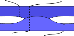
Define as the set
| (84) |
We claim that , see Figure 4. We test this against cylindrical sets , with and Borel:
| (85) | ||||
Here we used (79), (80), Fubini’s theorem, and the change of variables formula. The claim is shown. In particular, . It follows that and for every , since , whereas by Prokhorov’s theorem as . All in all, .
Finally, we have to estimate the action. Outside of the membrane, this is simply Jensen’s inequality:
| (86) |
Inside the membrane, we first note that is absolutely continuous with respect to , with density
| (87) |
so that
| (88) |
∎
Example 6.5.
Consider and set and . This is an optimal curve connecting its two end points. The flux is and the cost is simply .
Another optimal curve is given by , . This curve is also optimal, with the same flux and cost .
For , the optimal curve between and is supported on the curves
| (90) |
with and . The distribution of crossing coordinates then minimizes
| (91) |
among all probability measures. A simple calculation shows that
| (92) |
with chosen uniquely so that is a probability measure. We note that for , the only crossing point is , and we recover .
7 Homogenization
In this section we prove Theorem 1.2, i.e. we will show that -converges to .
Let us start by collecting a few properties of the functional defined in (10).
Lemma 7.1.
The following properties hold:
-
(i)
For all there exist minimizers and of .
-
(ii)
The map is convex, lower semicontinuous, and -homogeneous in .
-
(iii)
is convex and lower semicontinuous.
-
(iv)
There is a constant depending only on and such that for all , .
-
(v)
If then .
-
(vi)
With as above,
(93) for all , . In addition, is locally Lipschitz in .
Proof.
First note that . We take minimizing sequences , . Then almost everywhere and . By the Banach-Alaoglu Theorem there exists a subsequence converging weakly- in to some satisfying almost everywhere and . Since , we also get a subsequence in , with in and . By the convexity and lower semicontinuity of the function and Mazur’s Lemma, we have
| (94) |
which shows that are minimizers.
These properties are inherited from the function .
This is the result of Lemma 2.1.
The lower bound follows from Jensen’s inequality. For the upper bound, consider the vector field from Lemma 7.2 below, and find such that almost everywhere in , and . Then
| (95) |
The lower bound is shown in . For the upper bound, take and .
This follows from and : Let . Then
| (96) |
so that .
To see the first inequality, start with a minimizer . Then is a competitor for .
To see the second inequality, start with a minimizer . Then is a competitor for .
Together with the growth condition (iv) we obtain the local Lipschitz property on . ∎
The following lemma turns out to be crucial.
Lemma 7.2.
There is a constant depending only on such that for every there is a vector field such that in , , and .
Proof.
Let be a Lipschitz curve. Define the vector-valued measure . Then in , , and .
Let . By the conditions on , there are Lipschitz curves , , such that , , and .
Define , where is a standard mollifier. We note that is -periodic, , , and , where we used Young’s convolution inequality and the finite overlap of the curves . The projection of to inherits all the relevant properties. ∎
We need the following lemma to estimate corrector errors.
Lemma 7.3 (Local Poincaré-trace inequality).
There are constants , depending only on such that for any , , , we have
| (99) |
Here .
This differs from the standard Poincaré-trace inequality (see e.g. Theorem 12.3 in [15]) in that the smaller cube is not connected, nor is either cube Lipschitz-bounded.
Proof.
The statement is independent of . We only have to show it for and .
We take as any number such that all are connected by a rectifiable path in .
Assume that for this choice of , no such exists. Then there exists a sequence and a sequence such that , , and .
Because is Lipschitz bounded, we can cover with finitely many open rectangles such that, up to a rigid motion, , where is Lipschitz.
From [15, Theorem 12.3], we infer that there exists a bounded linear extension operator such that almost everywhere in and
| (100) |
Note that only appears on the right-hand side since we are not looking for a global extension.
Extending each using this operator, we extract a subsequence (not relabeled) such that , in , and in . Also, the traces converge in to the trace .
It follows that is piecewise constant. Because any two points in are path-connected in the domain, is constant in . Because , almost everywhere in . However, we have
| (101) |
a contradiction. ∎
We note that this implies the usal Poincaré-trace inequality in particular for -periodic functions in .
Finally we prove Theorem 1.2.
7.1 Proof of Theorem 1.2
Proof of the lower bound.
We start with a sequence of curves with , together with a sequence of momentum fields , such that in and
| (102) |
Step 1: We consider instead averaged versions defined through
| (103) | ||||
Here are first extended for constantly and by respectively, and is the discrete heat kernel for at time .
The averaged versions have the following properties:
| (104) | ||||
We note that and in , and by the convexity of the function , we have
| (105) |
Step 2: Define for the cube . Define and . Note that in . We now find a competitor for for almost every :
Consider the Hilbert space of -periodic functions with mean , equipped with symmetric bilinear form , which is independent of and positive definite by Lemma 7.3.
By the Lax-Milgram theorem, we may thus find for every a weak solution of
| (106) |
for every . Moreover, through integration by parts, using Hölder’s inequality and Lemma 7.3, we may estimate
| (107) | ||||
where we used the fact that is -periodic and that on in the sense of distributions.
Inserting the solution into (LABEL:eq:_estimate_Lax) and using the estimates in (104), we find through Fubini’s theorem and Hölder’s inequality that for every we have
| (108) |
Further, the vector field can be extended periodically to all of and then by 0 in , and the extension has zero distributional divergence in by (106). It follows that
| (109) |
We also use inequality from Lemma 7.1 to obtain
| (110) | ||||
Integrating over yields
| (111) | ||||
where we used Jensen’s inequality and the convexity of the function for the first term, and the lower bound in for the second.
Proof of the upper bound.
We have to show that for all curves of measures there exists for every a curve of measures such that as we have for all and
| (115) |
Step 1: We may assume that has finite energy. We mollify
in time and space with a standard mollifier. Let us call this curve and the corresponding optimal
momentum vector field .
Step 2: We fix a number of time steps satisfying . We define for and the following objects
| (116) | ||||
Note that for with the linear interpolation between and
| (117) |
Step 3: We insert the optimal microstructures and for , where
| (118) |
Fix to be chosen later, and define for
| (119) | ||||
where , is the positive lower bound of the function , is the discrete heat flow on
, and is the vector field from Lemma 7.2.
Step 4: For we define and as the linear interpolations
| (120) | ||||
We see that
| (121) |
where denotes the jump of from to . Note that since , by Fubini’s theorem the above is defined for almost every .
Moreover, for every we have
| (122) |
and
| (123) |
Combining the above with (117), we also obtain that
| (124) |
or more concisely
| (125) |
for every , for almost every . Note that in (125) it is imperative that be the half-open cubes.
Step 5: Let be the weak solution to
| (126) |
i.e. the unique function in the Hilbert space with
| (127) | ||||
for all . Note that after extending by in , (LABEL:eq:_weak_form) actually holds for all .
By the Lax-Milgram Theorem, a unique such exists for almost every . Testing with and using Lemma 7.3, we see that
| (128) | ||||
At this point we pick such that , which is possible by Fubini’s theorem and the regularity of the discrete heat flow. Of course, , so that
| (129) |
Further, taking , we see by (LABEL:eq:_weak_form) that in .
Step 6: We estimate using (129) that
| (130) | ||||
Using the joint convexity of the function we find for that
| (131) | ||||
We estimate using Lemma 7.2:
| (132) | ||||
For the main term we find through exploiting the convexity and the definition of that
| (133) |
Finally, we use the Lipschitz continuity of from Lemma 7.1 and the Lipschitz continuity of to estimate the Riemann sum above by the integral
| (135) |
Choosing and letting we otain the desired estimate
| (136) |
where we used the convexity of in the last equality (Lemma 7.1). Finally take a diagonal sequence such that for all . ∎
Remark 7.4.
Finally, we note that we may add lower bounds on the density, in the form for every closed set , with a measurable lower density bound , with almost everywhere. This is just another convex constraint.
In fact, Theorem 1.2 can be proved under the additional constraint for with a few easy modifications. In (11), we take the infimum with the additional constraint that almost everywhere, increasing the energy.
In Lemma 7.1, the upper bound in (iv) then has to be replaced by
| (137) |
References
- [1] Luigi Ambrosio, Gianluca Crippa, Camillo De Lellis, Felix Otto, and Michael Westdickenberg. Transport equations and multi-D hyperbolic conservation laws, volume 5 of Lecture Notes of the Unione Matematica Italiana. Springer-Verlag, Berlin; UMI, Bologna, 2008. Lecture notes from the Winter School held in Bologna, January 2005, Edited by Fabio Ancona, Stefano Bianchini, Rinaldo M. Colombo, De Lellis, Andrea Marson and Annamaria Montanari.
- [2] Luigi Ambrosio, Nicola Fusco, and Diego Pallara. Functions of bounded variation and free discontinuity problems. Oxford Mathematical Monographs. The Clarendon Press, Oxford University Press, New York, 2000.
- [3] Jean-David Benamou and Yann Brenier. A computational fluid mechanics solution to the Monge-Kantorovich mass transfer problem. Numerische Mathematik, 84(3):375–393, 2000.
- [4] Jean-David Benamou, Guillaume Carlier, and Filippo Santambrogio. Variational mean field games. In Active Particles, Volume 1, pages 141–171. Springer, 2017.
- [5] Andrea Braides. Gamma-convergence for Beginners, volume 22. Clarendon Press, 2002.
- [6] Andrea Braides and Anneliese Defranceschi. Homogenization of multiple integrals, volume 12. Oxford University Press, 1998.
- [7] Andrea Braides, Irene Fonseca, and Giovanni Leoni. A-quasiconvexity: relaxation and homogenization. ESAIM: Control, Optimisation and Calculus of Variations, 5:539–577, 2000.
- [8] Giuseppe Buttazzo, Chloé Jimenez, and Edouard Oudet. An optimization problem for mass transportation with congested dynamics. SIAM Journal on Control and Optimization, 48(3):1961–1976, 2009.
- [9] Pierre Cardaliaguet, Alpár R Mészáros, and Filippo Santambrogio. First order mean field games with density constraints: pressure equals price. SIAM Journal on Control and Optimization, 54(5):2672–2709, 2016.
- [10] Gianni Dal Maso. An introduction to -convergence, volume 8. Springer Science & Business Media, 2012.
- [11] Lester Randolph Ford Jr and Delbert Ray Fulkerson. Flows in networks. Princeton university press, 2015.
- [12] Gero Friesecke, Richard D. James, and Stefan Müller. A theorem on geometric rigidity and the derivation of nonlinear plate theory from three-dimensional elasticity. Communications on Pure and Applied Mathematics, 55(11):1461–1506, 2002.
- [13] Richard Jordan, David Kinderlehrer, and Felix Otto. The variational formulation of the Fokker–Planck equation. SIAM journal on mathematical analysis, 29(1):1–17, 1998.
- [14] Jonathan Korman and Robert McCann. Optimal transportation with capacity constraints. Transactions of the American Mathematical Society, 367(3):1501–1521, 2015.
- [15] Giovanni Leoni. A first course in Sobolev spaces. American Mathematical Soc., 2017.
- [16] Jian-Guo Liu, Robert L Pego, and Dejan Slepčev. Euler sprays and Wasserstein geometry of the space of shapes. arXiv:1604.03387, 2016.
- [17] Jian-Guo Liu, Robert L. Pego, and Dejan Slepčev. Least action principles for incompressible flows and geodesics between shapes. Calc. Var. Partial Differential Equations, 58(5):Paper No. 179, 43, 2019.
- [18] Pierre Moerbeke. On optimal stopping and free boundary problems. Archive for Rational Mechanics and Analysis, 60(2):101–148, 1976.
- [19] Felix Otto. The geometry of dissipative evolution equations: the porous medium equation. 2001.
- [20] Christopher Priest. The Prestige. Touchstone, Simon & Schuster, 1995.
- [21] Philip E Protter. Stochastic differential equations. In Stochastic integration and differential equations, pages 249–361. Springer, 2005.
- [22] S. K. Smirnov. Decomposition of solenoidal vector charges into elementary solenoids and the structure of normal one-dimensional currents. St. Petersburg Mathematical Journal, 5(4):841–867, 1994.
- [23] Torsten Teorell. Studies on the “Diffusion Effect” upon ionic distribution. Some theoretical considerations. Proceedings of the National Academy of Sciences of the United States of America, 21(3):152, 1935.
- [24] Juan Luis Vázquez. The porous medium equation: mathematical theory. Oxford University Press, 2007.