Learning to Weight for Text Classification
Abstract
In information retrieval (IR) and related tasks, term weighting approaches typically consider the frequency of the term in the document and in the collection in order to compute a score reflecting the importance of the term for the document. In tasks characterized by the presence of training data (such as text classification) it seems logical that the term weighting function should take into account the distribution (as estimated from training data) of the term across the classes of interest. Although “supervised term weighting” approaches that use this intuition have been described before, they have failed to show consistent improvements. In this article we analyse the possible reasons for this failure, and call consolidated assumptions into question. Following this criticism we propose a novel supervised term weighting approach that, instead of relying on any predefined formula, learns a term weighting function optimised on the training set of interest; we dub this approach Learning to Weight (LTW). The experiments that we run on several well-known benchmarks, and using different learning methods, show that our method outperforms previous term weighting approaches in text classification.
Index Terms:
Term weighting, Supervised term weighting, Text classification, Neural networks, Deep learning.1 Introduction
In information retrieval (IR) and related disciplines, where each textual document is represented as a vector of terms (a.k.a. “features”), term weighting consists of computing a numerical score that reflects the importance of a given term for a given document [1]. Once the designer has decided what should constitute a “term” (e.g., a word, or the morphological root of a word, or a character -gram, etc.), and has thus decided what a vector consists of in the system, the term weighting method is responsible for filling out the vector that will represent a specific document. Once filled, this vector is fed to the module responsible for computing document-document similarity (when ad hoc search, or text clustering, are the tasks of interest), or to the module responsible for training a classifier, or to the classifier itself (in the case of text classification). Different term weighting methods generate different vectors for the same document, thus attributing to the document different semantic interpretations. “Good” term weighting methods are thus of fundamental importance for delivering good search/clustering/classification accuracy.
Term weighting approaches widely used in IR include TFIDF and BM25; loosely speaking, both methods (as long as practically all other term weighting methods in the literature) rely on the same principles, i.e., (a) that terms that occur more frequently in the document (i.e., terms with high “term frequency”) are more relevant to the document, and (b) that terms that occur in fewer documents (i.e., terms with high “inverse document frequency”) are more relevant tout court. Different interpretations of these principles lead to the many term weighting formulae proposed in the literature [2, 1, 3]. However, practically all such formulae share a common structure. To see this, let us take one of the many variants of TFIDF, i.e.,
| (1) |
and let us take BM25, i.e.,
| (2) | ||||
as examples. Here, is the term and is the document for which the score is being computed, is the collection of documents (or: the set of training documents, in a text classification context), is the raw frequency (i.e., the number of occurrences) of term in document , is the number of documents containing the term, and are the length of (i.e., the number of term occurrences that contains) and the average length of the documents in , and and are two parameters (typically set to 1.2 and 0.75, respectively [4]). Leaving aside the mathematical details for the moment being, the important thing to note is that the right-hand side of both equations consists of the product of two factors, i.e., a document-dependent factor (the leftmost one), which depends on the term’s frequency in the document [5], and a collection-dependent factor (the rightmost one), which depends on the rarity / specificity of the term in the collection [6]. Accordingly, many term weighting functions share the common structure
| (3) |
where and are two “abstract”, generic functions representing the document-dependent and the collection-dependent factors, respectively111The parameter in and represents the set of classes, and is thus relevant only in text classification (or related) contexts. While functions used in ad hoc retrieval, such as those of Equations 1 and 2, do not depend on it, we include this parameter because it will prove useful when discussing instantiations of Equation 3 in text classification contexts.. Aside from these two factors, in many term weighting functions there is a third component in the weighting process, i.e., the normalisation component [7, 8, 3], whose aim is to factor out document length. In variants of Equation 1 it often takes the form of a denominator that normalises the entire function, e.g., implementing cosine normalisation; in Equation 2, instead, a normalisation component is already present in the denominator of the first factor.
The weighting functions of Equations 1 and 2 are unsupervised, i.e., they do not leverage the class labels of the training data when these latter are available. However, in tasks (such as text classification) characterised by the presence of training data it seems logical to think that one could take advantage of the information contained in these labels; this is the principle at the basis of Supervised Term Weighting (STW) [9]. The main intuition that underlies STW is that, in the presence of training data, the factor in Equation 3, which measures the discrimination power of term independently of any particular document , can be instantiated by means of a function that measures such discrimination power in a manner more specific to the task at hand (e.g., classification). In other words, while a traditional unsupervised function reflects the distribution of in the collection (and does not depend on the class labels ), STW replaces it with a function that reflects this distribution conditioned on ; in this way, a higher weight is thus given to those terms whose distribution in the training data is better correlated with the distribution of the labels.
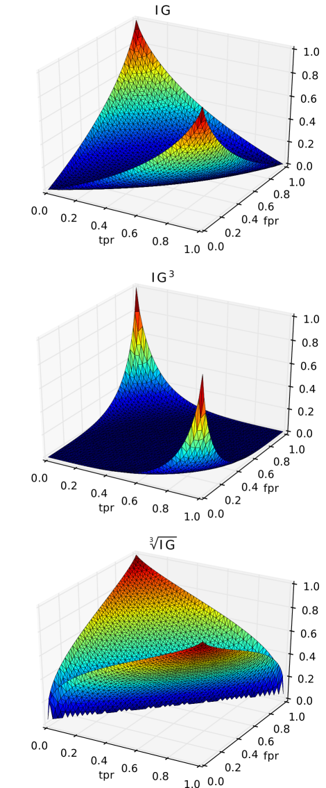
Several metrics could be directly borrowed from the literature as candidates for this supervised factor. Of particular interest are the feature-scoring functions (hereafter: “FS functions”) used in “filter-style” feature selection [10, 11]. Previous work in STW [12, 9, 13, 14, 15] has focused on identifying a FS function that performs well when used to instantiate the factor in Equation 3; the most widely used such functions include chi-square (denoted ), which evaluates the mutual statistical dependence of two random variables, and information gain (a.k.a. mutual information, see Equation 4), which measures the reduction in the entropy of one random variable (here: the class label) caused by the observation of another variable (here: the presence/absence of the term).
In STW, the component of Equation 3 is instantiated by one of these FS functions (e.g., information gain); unlike the second factors of Equations 1 and 2, these feature-scoring functions do depend on , i.e., on the set of classes of interest. In this article we will restrict our attention to the binary classification case, where (with indicating the complement of class ); we leave the extension to the multiclass case (i.e., ) to future work.
Despite the fact that all STW methods (a) do have an intuitive basis, and (b) have shown some success in empirical evaluations, there are no clear indications that one of them is consistently superior to the others. This means that a system designer has to resort to a trial-and-error method on a validation set in order to select the best-performing weighting criterion for the application of interest. This absence of a clear winner in the supervised term weighting camp may indicate that STW is yet to be fully understood; we attempt to provide some deeper insight on the nature of STW in Section 3.
In this article we propose a STW framework for text classification that learns the function from the training data; we call this framework Learning to Weight (LTW). The rationale behind LTW is that past work on term weighting (either unsupervised or supervised) suggests that whether a specific function is optimal or not is data-dependent, which means that it may be better to directly learn the optimal function from the data.
We propose various instantiations of this framework, each of them relying on neural network models that learn this function via optimization. It is important to remark that our goal here is not producing word embeddings or dense representations of documents. Instead, we resort to neural networks as a means of learning the optimal STW function that is to be applied to each (nonzero) element of a sparse vector of term frequencies. In order to gain generality, the optimization process we propose is independent of the learning algorithm used for training the classifier (and of the loss minimized by this algorithm), and is instead based on solving the simpler auxiliary problem of improving the linear separation between the positive and negative examples. The experiments we have conducted show that our method outperforms previous term weighting approaches for text classification. Furthermore, our exploration of the learned function brings about some interesting insights on the geometrical shape of the “ideal” function.
The remainder of the article is structured as follows. Section 2 reviews previous work on supervised term weighting, while Section 3 analyses the problems inherent in term weighting for text classification. Section 4 presents our LTW approach, followed by Section 5 in which we discuss the experimental evaluation we have carried out. In Section 6 we discuss whether it might make sense to also learn, aside from the factor, also the factor. Section 7 concludes and outlines possible avenues for future research.
2 Related Work
The history of term weighting goes back to the earliest vector-based models and probabilistic models of IR, which were developed in the ’60s (see e.g., [16, §3]). Two contributions that have withstood the test of time, and that form the basis of nowadays’ term weighting functions, are the two notions that we have already discussed in Section 1, i.e., term frequency (whose origins can be traced back to the development of the SMART system [17]) and inverse document frequency (which was first formalized in [6]). Many variants of Equations 1 and 2, which both combine the two notions in one single formula, have been developed over the years and tested against each other (for two large-scale comparisons see [1, 3]). While these two notions were originally devised for text search, over the years they have been adopted in an essentially unchanged form for other text mining tasks, such as text clustering (see e.g., [18]) and text classification (see e.g., [19, §5.1]).
Supervised term weighting. While this “acritical” adoption seems justified for clustering, which is unsupervised in nature, it seems not for classification, where additional information useful for weighting purposes can be extracted from training examples. This idea is at the heart of supervised term weighting. STW goes back to 2003, when Debole and Sebastiani [9] proposed to reuse the scores obtained from FS functions during (supervised) feature selection, in order to instantiate the factor of Equation 3, i.e., as a substitute of the more conventional and factors of Equations 1 and 2. The three variants investigated in that work used chi-square (Equation 4), information gain (Equation 5), and gain ratio (Equation 6) as instances of , i.e.,
| (4) | |||||
| (5) | |||||
| (6) |
where and denotes a probability on the event space of documents (e.g., is the probability that a random training document does not contain and belongs to class ). However, their results (using Support Vector Machines as the learning algorithm) did not show STW to bring about consistent improvements over TFIDF.
A subsequently proposed STW approach is ConfWeight [13], which adopts a relevance criterion based on statistical confidence intervals; the criterion can simultaneously be used for performing feature selection and term weighting. At the same time, [20] proposed relevance frequency, refined in [14] as
| (7) |
as the instance of the factor. STW based on relevance frequency (which we use as a baseline in the experiments of Section 5) was found by [20] to be superior to STW using or , but comparable to standard TFIDF under certain circumstances.
Experiments similar to the ones of Debole and Sebastiani [9] were carried out in [12], where instead STW proved useful for improving the classification accuracy of -Nearest Neighbours (KNN) classifiers.
Other variations on the same theme are to be found in [21, 22, 23, 24, 25], while applications of STW to specific instantiations of text classification, such as question classification [15] or sentiment classification [26, 27], have also been reported.
Overall, the results reported in the literature show, as hinted above, that there is no clear consensus as which variant of STW is the best, and as to whether STW is indeed superior or not to standard unsupervised weighting.
Representation learning. Term weighting document vectors is inherently related to representation learning, an area of research where neural networks, and in particular deep learning architectures [28], tend to outperform the competition. Deep learning allows computational models composed of non-linear projections to learn effective representations of the inputs by backpropagating the errors with respect to the model parameters. In recent work [29] deep learning models have been used to obtain continuous, dense representations for words and document vectors. Such methods have proved effective at modelling word semantics, but require the processing of very large external text collections in order to succeed. Bag-of-words approaches to text classification, which are the context of our LTW work, do not require any external text collection. In the experiments we include a comparison with FastText [30, 31], a top-performing method based on distributional semantics that uses dense representations.
In the present work neural networks are not used for training a text classifier (for this, a neural network or any other learning algorithm could be used); instead, the rationale of using neural networks is (a) to exploit their modelling flexibility in order to improve the weighting criterion, and (b) to permit the inspection of the learned weighting function, in order to allow the experimenter to gain intuitions on how an ideal such function looks like.
Learning term weights.. To the best of our knowledge, the Combined Component Approach (CCA) is the only previous approach resembling the idea of learning term weighting functions. CCA was presented in [32], in the context of learning to rank. CCA follows a radically different approach, though, based on composing, via genetic programming optimization, complex ranking functions from 20 weighting factors well-known from past literature (e.g., tf and idf variants, among others) used as the atomic components. Differently from [32], instead of exploring the (huge – see [3]) space of combinations of previously proposed weighting factors, we take the simpler tpr and fpr statistics (see Section 4) as the atomic components, and allow the optimization procedure full freedom. The main difference between CCA and our method is thus the fact that we use the supervision directly as input to the weighting function learning method (in order to compute the tpr and fpr statistics), while CCA only uses the supervision in the evaluation phase, i.e., their optimization procedure works primarily by composing unsupervised weighting factors. We include CCA as one of our baselines in the experiments of Section 5.
3 Pitfalls in Supervised Term Weighting Functions
In this section we analyse some of the typical instantiations of the components of supervised term weighting functions, trying to shed some light on the possible reasons why there is no consensus yet on which among the many available variants is preferable.
3.1 The Factor
The most frequently used unsupervised variants of the factor of Equation 3 include the raw frequency of in (Equation 8) and log-scaled versions of it (Equations 11 and 12):
| (8) | |||||
| (11) | |||||
| (12) |
In this paper we focus on the function; this allows us to draw a fair comparison with existing STW methods, which do not address the component of the weighting function. However, in this section we would like to discuss a few minor issues that affect traditional implementations of the function.
The linear version of Equation 8 does not take into account the fact that a term frequency variation at low frequency values, e.g., from 1 to 3, should be considered much more relevant than a term frequency variation at high frequency values, e.g, from 11 to 13. For this reason log-scaled versions such as those of Equations 11 and 12 are usually preferred, since they better capture frequency variations observed at low frequency values.
However, the non-linearity of log-scaled versions causes issues with document length. To illustrate this, let us consider a document and a document which consists of two juxtaposed copies of . The value of is double the value of ; since the log transformation is non-linear, if we use Equation 11 or Equation 12 the cosine-normalised vectors of and will not be the same, potentially clashing with the so-called “normalisation assumption”, according to which “for the same quantity of term matching, long documents are no more important than short documents” [3].
3.2 The Factor
FS functions have proven useful in filter-style approaches to feature selection [11]. Feature selection and term weighting are inherently related, as both tasks build upon a model of feature importance, which is what FS functions aim to measure. One might thus expect FS functions to fit the purposes of term weighting (an intuition that has driven a lot of previous work in STW – see Section 2). However, there are reasons to believe that a good FS function is not necessarily a good component of a term weighting function. The reason is that our notion of the quality of a FS function is typically based on its performance as a ranking function, since FS functions are customarily used in filter-style feature selection in order to rank features. That is, if is a FS function measuring the degree of importance of a feature (whatever this might mean), filter-style feature selection consists of taking the top ranked features according to their score.
Note that the numeric values produced by a FS function can be substantially modified by applying to them any monotonic non-decreasing function, without affecting the resulting rankings. For example, the three variants of the function in Figure 1 produce exactly the same results when used to rank features, but can result in very different outcomes when used to instantiate the function. This indicates that, when used in a supervised term weighting formula, for any FS function there is an additional dimension to be explored for optimization, i.e., monotonic non-decreasing transformations. Instead of systematically exploring the space of possible such transformations we propose to learn the weighting function from scratch on the training set, without relying on predefined term relevance functions. This proposal will be detailed in the next section.
4 Learning to Weight
We propose a novel supervised weighting approach that, instead of relying on any predefined formula, learns a term weighting function optimised on the available training set; we call this approach Learning to Weight (LTW)222We should remark that we do not optimise the weighting function for a specific test set. The fact that we do not use the test set in any way while learning the weighting function sets our approach apart from the realm of transductive learning, and squarely places it within the domain of inductive learning.. Essentially, during training, different term weighting functions (leading to different term weights for the same term-document pair) are tested, and the function that minimizes the linear separation between the positive and negative examples of the training set is chosen. The different term weighting functions that are tested are generated by neural architectures described in Section 4.1.
In the rest of the paper we will use slightly different mathematical conventions from the ones used in Section 2. In fact, while the four functions discussed in that section are all formulated in terms of the four variables , in reality they are functions of just two free variables, since the frequency of the class in the training set is fixed, and since and . In the rest of the paper we will thus express our functions in terms of just two free variables; however, consistently with the tradition of ROC analysis [33], as our two free variables we will equivalently choose the true positive rate
| (13) |
and the false positive rate
| (14) |
As a side effect, this change of variables makes it possible to plot any function in 3D space, which allows the experimenter to quickly gain an understanding on how the weights are assigned (something that will prove useful in our analysis of the results in Section 5). Figure 2
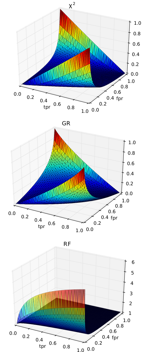
plots the FS functions discussed in Section 2 as a function of the two variables and of Equations 13 and 14; note that we have not plotted since it differs from by a fixed multiplicative factor only. As expected, the plots reveal a consensus on the higher importance of positively correlated terms (those characterized by high and low ). Interestingly enough, there are instead discrepancies among these functions on (i) how to assess the importance of negatively correlated terms (those with low and high ), which are considered as important as the positively correlated ones by functions and but ignored by ; or on (ii) how much the importance of the term changes due to variations in and .
4.1 Learning the Factor
In this work we will learn a weighting function individually for each binary classification problem. As discussed in Section 2, in the binary case any function of a contingency table can be expressed as a function of the two values and . Our working hypothesis is that the optimal such function is data-dependent. We thus propose to use a neural network to learn this function from data, since neural networks are universal approximators [34].
Concretely, we adopt a multi-layer feedforward network with one hidden layer, since this architecture, despite being simple333As part of this framework, more complex architectures could be adopted as well; however, this goes beyond the scope of this work (for which the expressive power of the adopted network is sufficient) and is something we plan to investigate in the future., is known to be able to approximate any continuous function if enough hidden nodes are considered [34].
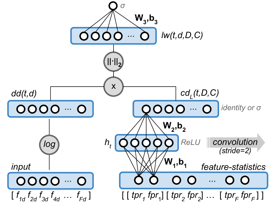
The computation we propose444Note the difference in notation between the function of Equation 3 and the functions of Equations 15 and 16; the former is an “abstract” function that measures the importance of term for dataset and set of classes , while the latter are concrete instantiations of it that we use in this paper. Similarly for the function of Equation 3 and the function of Equation 17. is described by the following equations:
| (15) | ||||
where is the output of the hidden layer, is the Rectifier Linear Unit activation function, is a vector of the two precomputed values and , respectively, and (for ) are the transformation matrix and the bias term, and is the logistic function. The model parameters and (for ) are shared across the model, i.e., the same set of parameters is used in order to compute the weight of each term, in a convolution-like manner (i.e., all scores are computed in parallel on each input pair – see the right branch of the network in Figure 3(a)). The subscript stands for feature-local, since the weight for a feature is computed from statistics ( and ) local to that feature.
Traditional STW approaches have only considered the local features as the inputs in order to compute the score. However, one could think of leveraging the global information in the collection in an attempt to model the possible inter-dependencies among features. For example, one could think of increasing the score for a feature which, despite not being too strongly correlated to the class label, has the strongest correlation among all other features. Note that such kind of considerations remain out of reach for all feature-local methods.
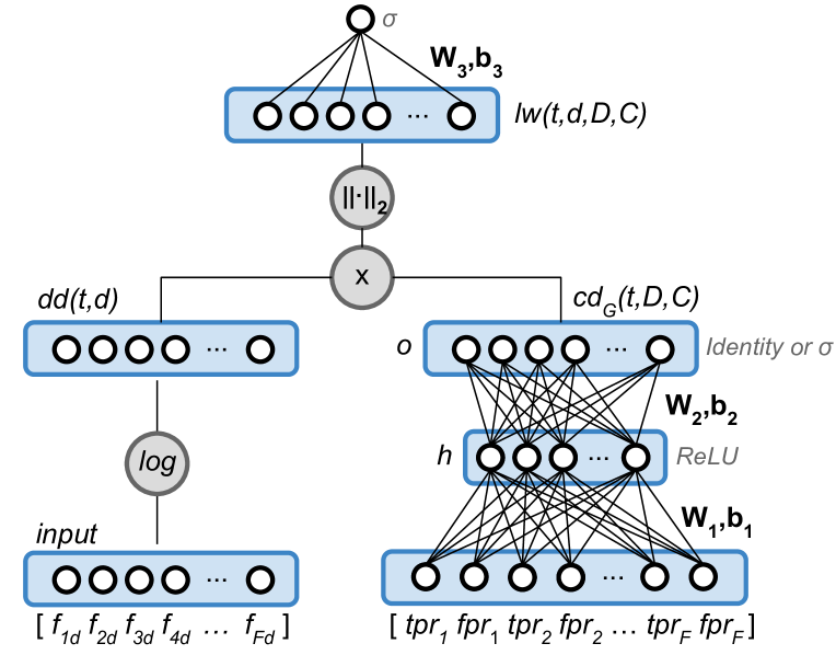
We thus propose an alternative model, dubbed feature-global, which instead uses the statistics of all features in order to compute the score of a given term. This variant is described by the set of equations
| (16) | ||||
where and (for ) are the model parameters (with the same meaning as above) and is the output vector containing all scores; the for term is returned via the operator. In this setup the hidden state is not the result of a separate parallel computation for each feature, but is instead the output of a single-step computation that takes into account all the features at the same time (Figure 3(b)).
Note that, as the input features for the function, we could opt for the four joint probabilities , in place of the factors. However, this would unnecessarily complicate the system, roughly doubling the number of parameters and additionally constraining it to discover the actual degrees of freedom in the input data. Conversely, using both and (and not, say, just one of them) is essential because and are altogether defined in terms of all four joint probabilities ( is a function of and while is a function of and ). If a method used only one of and , it would work with incomplete information about how are are correlated.
As a final note, all and inputs for the function (both local and global) are calculated once, at the beginning, and then fixed during all the optimization process. Note thus that the only part that varies during the training process concerns the term frequencies of each used document vector (i.e., the input of the function) which is not directly connected to the part. For more discussion on this see Section 7.
4.2 Composing the score
In this study we instantiate the factor with the function
| (17) |
i.e., a log-scaling of the frequencies of terms normalized by the document-length (). Normalizing by the document length is a simple way to limit the variation of the input range to the neural network, at the same time avoiding the issues related to document length (see Section 3.1).
Once the and factors are calculated, they are multiplied in a pointwise manner555Note that the tensor resulting from the branch has “shape” while the tensor from has “shape” . This mismatch in the pointwise multiplication is resolved via “broadcasting”, a typical operation in any deep learning framework. and then normalised via normalisation, i.e.,
| (18) |
where stands for learned weights and is either or .
The model parameters are optimised to improve the linear separability of the positive and negative examples. For that purpose we use a simple logistic regression model
| (19) |
where is the model prediction. As the loss function we use the cross-entropy
| (20) |
between the true label mapped into by means of
| (21) |
and the prediction logits . We use cross-entropy since it is known to be a good differentiable model of the error for logistic regression.
It is important to note that the logistic regression layer defined by and has the sole purpose of propagating the constraints on the parameters for the model. That is, the logistic regressor is merely used here as an auxiliary classifier, and the real output of the system are the parameters and (for ) of the function; the parameters and of the logistic regressor are set aside once the optimization ends. The choice of using a simple logistic regression layer is a minimalistic one, allowing to directly correlate the values of the function to the class labels, with minimal bias towards the actual classifier being used. Note that resorting to a more sophisticated classifier (e.g., a deep multi-layer feedforward network) could cause the contribution of the supervised factor to be diminished, as the (auxiliary) net could well end up delegating the modelling of complex aspects of the data to the inner layers. Stacking the simplest possible auxiliary classifier on top thus forces the quality of the layer (the actual outcome of the model) to be maximized.
Note that the Learning to Weight framework gives full control to the optimization process for balancing the different factors involved in the weighting process. For example, if a dataset can be easily separated by exclusively looking at the frequency of its terms, then the learning process will force the function to mimic the constant function . Otherwise, if the term frequency adds little information, the optimization process will try to compensate it by increasing the importance of the factor.
5 Experiments
In this section we experimentally compare our Learning to Weight framework to other supervised and unsupervised term weighting methods proposed in the literature666The code for reproducing all the experiments discussed in this paper is available at https://github.com/AlexMoreo/learning-to-weight.
5.1 Datasets
As the datasets for our experiments we use the popular Reuters-21578, 20Newsgroups, and Ohsumed corpora:
-
•
Reuters-21578 is a publicly available777http://www.daviddlewis.com/resources/testcollections/reuters21578/ test collection which consists of a set of 12,902 news stories, partitioned (according to the “ModApté” split we adopt) into a training set of 9,603 documents and a test set of 3,299 documents. In our experiments we restrict our attention to the 115 classes with at least one positive training example. After removing stopwords, the number of distinct terms amounts to 28,828. This dataset presents cases of severe imbalance, with several classes containing fewer than 5 positive examples.
-
•
20Newsgroups is a publicly available888http://qwone.com/~jason/20Newsgroups/ test collection of approximately 20,000 posts on Usenet discussion groups, nearly evenly partitioned across 20 different newsgroups. In this article we use the “harder” version of the dataset, i.e., the one from which all metadata (headers, footers, and quotes) have been removed (on this, see also Footnote 13). The dataset contains 101,322 distinct terms after removing stopwords.
-
•
The Ohsumed test collection [35] consists of a set of MEDLINE documents spanning the years from 1987 to 1991. Each entry consists of summary information relative to a paper published on one of 270 medical journals. The available fields are title, abstract, MeSH indexing terms, author, source, and publication type. Following [36], we restrict our experiments to the set of 23 cardiovascular disease classes, and we use (see http://disi.unitn.it/moschitti/corpora.htm) the 34,389 documents of year 1991 that have at least one of these 23 classes. Since no standard training/test split has been proposed in the literature we randomly partition the set into a part used for training (70% of the documents) and a part used for testing (the other 30%). The total number of distinct terms after removing stopwords is 54,949.
Since the present work deals with the binary case, each experiment on each of these test collections here consists of running as many binary classification tasks as there are classes in the collection.
5.2 Learning Algorithms
As the representation model, in all our experiments we use a simple unigram model with no stemming or lemmatization. All term weighting approaches are tested in exactly equal conditions, i.e., we run each combination of a term weighting method and a learning algorithm individually for each binary classification problem derived from each collection. In all cases, we apply local feature selection using as the feature scoring function and at a reduction ratio of 0.1; this has proven a good setting in text classification [11].
In order to assess the quality of the weighted vectors we consider the following learning algorithms for training classifiers:
-
•
Support Vector Machines (SVM) with a linear kernel [37], an algorithm that finds the hyperplane in high-dimensional spaces that separates, by the largest possible margin to the nearest training examples, the positive and negative examples.
-
•
Logistic Regression (LR), an algorithm that generates linear models of the probability that a document belongs to the class, by using the logistic function. Considering LR in our experiments is interesting because the LTW framework we define relies on LR to define the weighting function.
-
•
Multinomial Naive Bayes (MNB), which implements the naïve Bayes algorithm for multinomially distributed discrete data (though in text classification it is known to work well also for real-valued weighted vectors[38]).
-
•
K-Nearest Neighbours (KNN), an instance-based learning algorithm that outputs the class label more frequent across the examples most similar to the test example; as the measure of similarity we use the Euclidean distance.
-
•
Random Forests (RF), a method which builds an ensemble of decision trees. The implementation we use999http://scikit-learn.org/stable/modules/generated/sklearn.ensemble.RandomForestClassifier.html combines the resulting classifiers by averaging their probabilistic predictions, instead of returning the most frequent class output by the individual trees.
We also include the results of running FastText (FT – [30, 31]), a state-of-the-art method for text classification based on an evolution of the Word2Vec architecture [29, 39] for text classification. FastText is not a term weighting method and is here included for comparison purposes only, i.e., in order to verify how the text classification pipelines that we use in our experiments fare with respect to state-of-the-art text classification methods. Results for the FastText classifier are only reported for the dense representations that FastText produces, since in its currently available implementation it is not possible to use the FastText classifier with externally generated vectors.
5.3 Evaluation Measures
As the effectiveness measure we use the well-known , the harmonic mean of precision () and recall () defined as , where , , , are the numbers of true positives, false positives, false negatives, from the binary contingency table. We take when , since the classifier has correctly classified all examples as negative.
In order to average across all the classes of a given dataset we compute both micro-averaged (denoted by ) and macro-averaged (denoted by ). is obtained by (i) computing the class-specific values , , and , (ii) obtaining as the sum of the ’s (same for and ), and then applying the formula. is obtained by first computing the class-specific values and then averaging them across the classes.
5.4 Baseline Methods
We choose some relevant unsupervised and supervised weighting methods as the baselines against which to compare the Learning to Weight framework. The methods considered in this experimental evaluation are grouped as follows:
-
•
Unsupervised Term Weighting (UTW) methods: Binary (the simplest weighting function, that returns 1 if the document contains the term and 0 otherwise), TF (Equation 8), LogTF (Equation 11), TFIDF (a variant of Equation 1 that uses the raw frequency of Equation 8 as the component), LogTFIDF (Equation 1), and BM25 (Equation 2).
-
•
Supervised Term Weighting (STW) methods: TFCHI (Equation 4) and TFGR (Equation 6), proposed in [9]; ConfWeight [13], and TFRF (Equation 7), proposed in [14]. For all STW variants in this evaluation we adopt the factor defined in Equation 11. We leave aside TFIG (Equation 5) since, in binary classification, it is equivalent to TFGR, because the only difference between the two is a constant normalisation factor that is cancelled out by cosine normalisation. We also include the dense representations (Dense) that FastText produces in this group, since they are conditioned on the class labels [30, 31]. We also consider the CCA method discussed at the end of Section 2, suitably adapted to binary text classification, as a further STW baseline.
-
•
Learning to Weight (LTW): we consider both local (L – Equation 15) and global (G – Equation 16) versions for the factor. We also investigate a variant whereby the sigmoid activation function () of the factor is replaced by an identity function (I – thus allowing the model to output unbounded and negative scores). We thus propose four LTW variants; e.g., LTW-L- denotes LTW using the Local variant with the activation function.
5.5 Implementation Details
We have implemented our method using Tensorflow [40]. In our experiments we apply dropout to the hidden layer activations (with a drop probability of 0.2) in order to prevent overfitting. We use stochastic optimization relying on the Adam optimiser [41] with a learning rate of 0.005 (leaving the rest of the parameters set to their default values, i.e., , , and ), with a batch size of 100 and shuffling whenever an epoch is completed. We set the maximum number of iterations to 100,000 steps. However, we use an early stopping criterion, triggered when 20 consecutive validation steps (each of them run after every 100 training steps) have shown no improvement. In our experiments the runs obtain this convergence after an average of 5,780 steps, ranging from 900 to 18,100. The result scores that we report for all LTW variants are averages across 10 runs. For the model architecture we use a size of the hidden layer equal to 1000 for the local variant (which actually is the size of the convolutional filter that works on each feature separately) and a larger size of for the global variant, where is the number of distinct terms in the training set. The rationale behind using a larger size for the global variant is that it is also meant to model inter-feature relations.
For the learning algorithms other than FastText and CCA we use the implementations provided by Scikit-learn [42]. For FastText we use its publicly available implementation101010https://github.com/facebookresearch/fastText. As with all other learners, also with FastText we train independent binary classifiers, one for each class. We leave the learning rate at 0.1 (its default value). Although the authors recommend to set the epoch parameter (the number of times a complete pass over the entire set is to be performed) in the range [5,50], we have experienced a consistent improvement in performance across all datasets when using higher values. We thus vary the number of epochs in , and the best values turn out to be 100 for Reuters-21578 and Ohsumed, and 500 for 20Newsgroups (for which no further improvement is verified for higher values).
We have reimplemented111111Our implementation of CCA is accessible as part of our code release. the CCA method according to the specifications in [32], and adapted it to binary classification (in place of ranking, as it was originally devised for). This means replacing the ranking-oriented evaluation function used as the fitness function (originally, a combination of PAVG and FFP4) with , which is better suited for classification (and is also our evaluation measure of choice). We modify the process for the selection of the best individual so as to be driven by the classification accuracy of a logistic regressor121212The choice of logistic regression as a proxy has to do with efficiency. In fact, genetic programming is known to be computationally expensive, and most of its cost is accounted for by the evaluation of the fitness function. Since the classifier generated by logistic regression is an efficient one, this has a positive impact on the efficiency of this evaluation. as measured on a validation set. In our implementation of CCA we do not consider terminals and since they are inherently defined upon the notion of “query”, a notion that does not apply to text classification. All the hyper-parameters are set to the values recommended in [32].
To guarantee fair comparisons between our weighting methods and the baseline weighting methods, the parameters of each classifier are optimised individually, i.e., for each weighting method, learning method, binary class combination. For all such combinations, optimization is performed on a subset of the training set used as held-out validation set; once the parameter values have been chosen, the validation set is merged again into the training set and the classifier is retrained. For SVMs and LR we test values for the penalty parameter in the set , and alternatively consider the “dual” and “primal” optimization variants. For SVMs we test values for the loss parameter in . Adhering to a practice well documented in the literature, for SVMs we adopt the RBF kernel in the experiments in which dense vectors are used (i.e., in the experiments that use the representations produced by FastText, documented in rows “Dense” of Tables I and II), while we adopt the linear kernel when documents are represented by sparse vectors (i.e., all other experiments). For LR we test both L1 and L2 regularisation. For MNB, for the parameter we test all values in {0.0, 0.001, 0.01, 0.05, 0.1, 1.0}. For KNN, for the parameter we test all values in (a) with all features, or (b) with dimensionality reduction obtained by selecting the top features using the feature scoring function, or (c) with dimensionality reduction obtained via Principal Component Analysis (PCA) at dimensions. For RF we vary the number of trees in , we test both the Gini and Entropy criteria, and we consider a maximum number of features in , where is the total number of features.
5.6 Results
Tables I and II report the results we have obtained on the Reuters-21578, 20Newsgroups131313While some previous papers (e.g., [43]) have reported substantially higher scores for this dataset, it is worth noticing that we use a harder, more realistic version of the dataset than has been used in those papers. In our version, headers, footers, and quotes have been removed, since these fields contain terms that have near-perfect correlation with the classes of interest, thus making the classification task unrealistically easy; see http://scikit-learn.org/stable/datasets/twenty_newsgroups.html for further details. Our results are indeed consistent with those of other papers (e.g., [44]) which follow the same policy as ours., and Ohsumed datasets, for macro- and micro-averaged . Values in boldface indicate the best results obtained with the given learner on the given dataset, while values in greyed-out cells indicate the LTW variants that outperform all baselines.
| Reuters-21578 | 20Newsgroups | Ohsumed | |||||||||||||||||
| SVM | LR | MNB | KNN | RF | FT | SVM | LR | MNB | KNN | RF | FT | SVM | LR | MNB | KNN | RF | FT | ||
| UTW | Binary | .519 | .579 | .489 | .493 | .562 | – | .581 | .593 | .615 | .429 | .579 | – | .578 | .601 | .548 | .516 | .626 | – |
| TF | .592 | .599 | .490 | .496 | .555 | – | .583 | .579 | .601 | .418 | .578 | – | .593 | .606 | .540 | .530 | .634 | – | |
| LogTF | .569 | .612 | .449 | .522 | .558 | – | .611 | .619 | .571 | .470 | .570 | – | .620 | .632 | .453 | .550 | .638 | – | |
| TFIDF | .596 | .604 | .473 | .502 | .544 | – | .598 | .609 | .594 | .492 | .592 | – | .605 | .612 | .506 | .558 | .639 | – | |
| LogTFIDF | .576 | .609 | .462 | .496 | .530 | – | .607 | .622 | .580 | .512 | .583 | – | .614 | .636 | .491 | .574 | .643 | – | |
| BM25 | .554 | .582 | .462 | .509 | .561 | – | .602 | .621 | .572 | .536 | .588 | – | .607 | .634 | .473 | .576 | .637 | – | |
| STW | TFGR | .598 | .623 | .539 | .561 | .572 | – | .613 | .613 | .653 | .500 | .571 | – | .508 | .546 | .299 | .566 | .621 | – |
| TFCHI | .591 | .608 | .514 | .538 | .579 | – | .585 | .590 | .645 | .509 | .587 | – | .478 | .514 | .267 | .590 | .626 | – | |
| ConfWeight | .580 | .587 | .497 | .543 | .540 | – | .588 | .577 | .578 | .485 | .569 | – | .649 | .647 | .617 | .599 | .646 | – | |
| TFRF | .584 | .602 | .461 | .508 | .539 | – | .626 | .624 | .617 | .434 | .581 | – | .635 | .634 | .552 | .477 | .640 | – | |
| Dense | .541 | .537 | .508 | .565 | .547 | .553 | .574 | .572 | .539 | .582 | .585 | .566 | .618 | .619 | .533 | .620 | .617 | .617 | |
| CCA | .556 | .574 | .418 | .511 | .562 | – | .581 | .578 | .604 | .487 | .579 | – | .616 | .612 | .572 | .561 | .635 | – | |
| LTW | LTW-L- | .614 | .610 | .517 | .542 | .547 | – | .625 | .619 | .660 | .600 | .577 | – | .642 | .642 | .596 | .543 | .624 | – |
| LTW-L-I | .629 | .619 | .502 | .583 | .553 | – | .630 | .626 | .668 | .582 | .573 | – | .649 | .645 | .607 | .576 | .616 | – | |
| LTW-G- | .531 | .530 | .375 | .442 | .505 | – | .541 | .534 | .537 | .278 | .514 | – | .554 | .548 | .480 | .343 | .566 | – | |
| LTW-G-I | .604 | .604 | .374 | .555 | .540 | – | .635 | .620 | .494 | 573 | .571 | – | .651 | .650 | .459 | .638 | .633 | – | |
| Reuters-21578 | 20Newsgroups | Ohsumed | |||||||||||||||||
| SVM | LR | MNB | KNN | RF | FT | SVM | LR | MNB | KNN | RF | FT | SVM | LR | MNB | KNN | RF | FT | ||
| UTW | Binary | .822 | .843 | .649 | .794 | .841 | – | .595 | .609 | .623 | .449 | .595 | – | .642 | .639 | .589 | .547 | .663 | – |
| TF | .836 | .843 | .621 | .797 | .847 | – | .596 | .592 | .598 | .436 | .593 | – | .643 | .643 | .583 | .559 | .684 | – | |
| LogTF | .855 | .861 | .786 | .815 | .846 | – | .628 | .634 | .599 | .492 | .593 | – | .663 | .668 | .550 | .580 | .684 | – | |
| TFIDF | .852 | .850 | .787 | .818 | .839 | – | .617 | .627 | .619 | .511 | .612 | – | .659 | .612 | .574 | .581 | .681 | – | |
| LogTFIDF | .849 | .861 | .781 | .816 | .841 | – | .627 | .637 | .607 | .532 | .605 | – | .665 | .668 | .566 | .599 | .684 | – | |
| BM25 | .844 | .850 | .769 | .819 | .847 | – | .622 | .638 | .599 | .552 | .610 | – | .652 | .659 | .549 | .604 | .685 | – | |
| STW | TFGR | .846 | .854 | .821 | .815 | .849 | – | .630 | .631 | .667 | .516 | .589 | – | .577 | .587 | .410 | .596 | .664 | – |
| TFCHI | .836 | .839 | .798 | .805 | .846 | – | .601 | .607 | .659 | .516 | .602 | – | .566 | .588 | .379 | .616 | .665 | – | |
| ConfWeight | .823 | .821 | .754 | .808 | .834 | – | .603 | .592 | .609 | .495 | .593 | – | .668 | .677 | .657 | .635 | .682 | – | |
| TFRF | .862 | .864 | .790 | .804 | .840 | – | .643 | .637 | .644 | .452 | .602 | – | .677 | .662 | .619 | .536 | .679 | – | |
| Dense | .849 | .851 | .821 | .851 | .848 | .851 | .580 | .579 | .551 | .591 | .597 | .575 | .647 | .648 | .558 | .548 | .646 | .651 | |
| CCA | .837 | .841 | .623 | .406 | .838 | – | .600 | .601 | .605 | .507 | .597 | – | .672 | .673 | .615 | .595 | .685 | – | |
| LTW | LTW-L- | .867 | .865 | .825 | .819 | .848 | – | .645 | .636 | .685 | .603 | .597 | – | .688 | .678 | .660 | .598 | .663 | – |
| LTW-L-I | .874 | .869 | .821 | .843 | .846 | – | .649 | .643 | .690 | .586 | .593 | – | .688 | .680 | .665 | .622 | .650 | – | |
| LTW-G- | .824 | .818 | .773 | .776 | .819 | – | .555 | .546 | .563 | .292 | .536 | – | .601 | .595 | .555 | .419 | .615 | – | |
| LTW-G-I | .869 | .867 | .699 | 830 | .844 | – | .650 | .635 | .516 | .589 | .590 | – | .693 | .689 | .513 | .666 | .663 | – | |
The results indicate that most LTW approaches perform comparably or better than the baselines in terms of , and outperform the baselines in in most cases (statistical significance is discussed in Section 5.7). The best absolute classification result for each dataset is always obtained by LTW.
The local variants exhibit the most stable improvement across datasets and classifiers, while the global variants seem more unstable in this regard. The local variants outperform all other baselines on average in Reuters-21578 and 20Newsgroups (and rank second in Ohsumed); the LTW-L-I variant is overall the best-performing method. The LTW-G-I vectors produce competitive results when used in combination with SVMs, LR, and KNN. Conversely, the globally computed vectors prove less suitable for the MNB classifier; this may be explained by the fact that globally leveraging the dependencies between features contradicts the independence assumption built into the MNB classifier.
It is worth noticing that the unbounded versions (I) turn out to be more competitive than the bounded ones (). This seems to clash with the fact that traditional implementations of generate values that are always non-negative and usually upper-bounded by 1. However, allowing the score to be negative gives the optimiser the opportunity to discern between positive and negative correlation with the class, while most FS functions do not draw any distinction between these two cases. Furthermore, allowing the score to exceed the bounds [0,1] helps the optimiser to tune the relative importance of the and the factors.
Regarding the baselines, TFGR and TFCHI outperform the UTW approaches in most cases across Reuters-21578 and 20Newsgroups, but perform comparably worse in Ohsumed. This seems to indicate that, although traditional FS functions succeed in reflecting feature importance, some adaptation may be required in order to safely incorporate this score into the weight calculation. Binary is the worst-performing method (even though it works reasonably well with the MNB classifier – which was to be expected given that the classifier was originally designed with binary features in mind141414The particular implementation we use here is able to take advantage of real-valued vectors, though. See [38] for further details.). This is a consequence of the fact that binary weighting disregards term frequency (apart from mere presence/absence) and term specificity in the collection. Other things being equal, it is noteworthy that both UTW and STW perform irregularly across different conditions (e.g., in the STW group ConfWeight obtained the best average performance on Ohsumed but the worst on Reuters-21578 and 20Newsgroups), without any clear winner in the respective groups.
The dense representations generated by FastText perform comparably to the best-performing competitor in combination with KNN and RF classifiers in most cases. As a classifier, FastText (FT) performed irregularly across datasets, outperforming several baselines on Ohsumed, both in terms of and , but being surpassed by many UTW and STW methods in combination with SVM and LR on the other datasets. Those results seem to confirm that the superiority of deep learning models over traditional learners is only reached when learning from much larger text collections.
In our experiments CCA never stands out from the point of view of accuracy, obtaining scores which are almost always in-between the worst result and the best result obtained by the other methods. Despite the fact that CCA is somehow similar in spirit to LTW, in the sense that both frameworks aim at optimizing the term weighting function (following radically different strategies, though), the weighting functions produced by CCA are often too complex to interpret. In our experiments, the depth of the formulae (when viewed as trees of operators and operands) representing the weighting functions that CCA finds, range from a minimum of 1 to a maximum of 13; the mode of the distribution is 5, which already indicates fairly complex formulae.
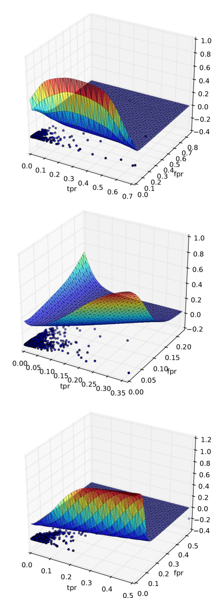
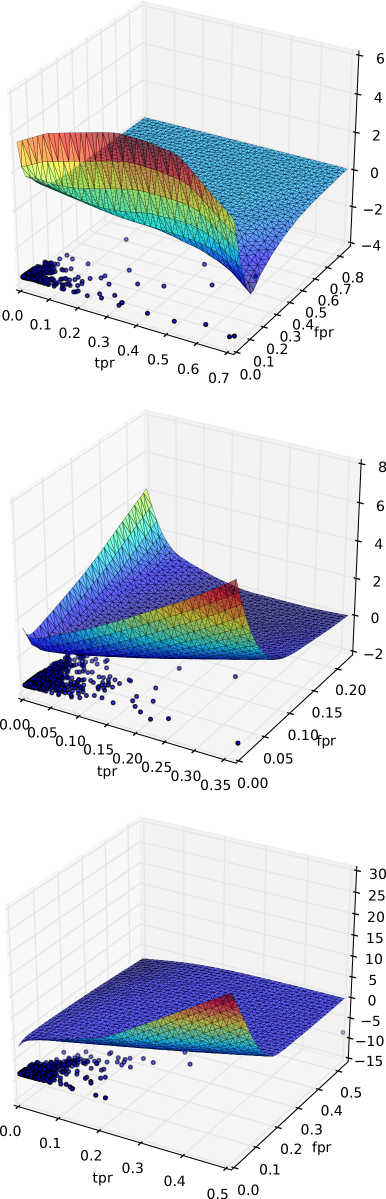
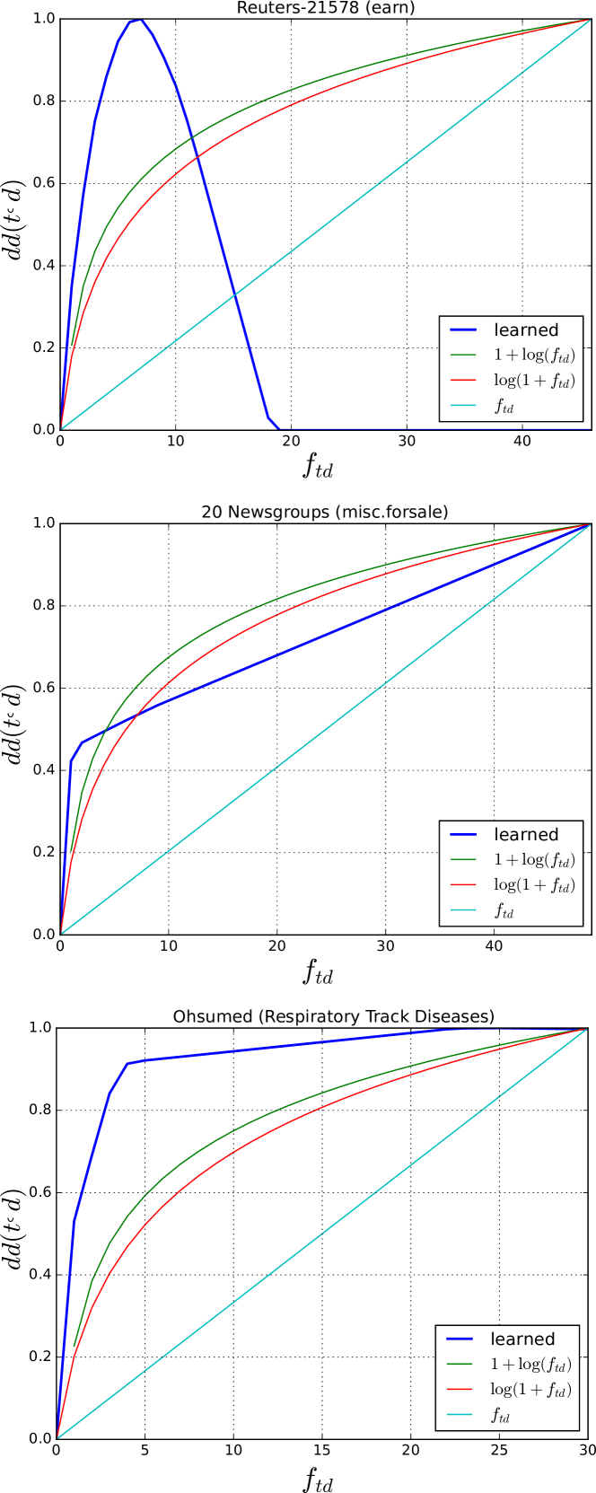
Figures 4(a) and 4(b) show examples of the learned local functions in their LTW-L- and LTW-L-I variants, respectively, for a sample class in each dataset. We also include the actual coordinates (,) for each of the features. (Similar plots cannot be displayed for the global variants since global functions depend on a larger number of coordinates.) Note that all learned functions agree that the most important terms are those characterized by a high and a very low . However, different cases give rise to different shapes151515We verified that the shapes are consistent through different runs, with negligible variations among them. In additional experiments we forced the function to mimic information gain in a pre-training phase. This had essentially no impact on the final shape.. The LTW-L-I versions tends to generate values that are sometimes higher than 1, and even smaller than 0 under certain conditions, e.g., when moves away from low values (see Figure 4(b), top) or when has very low values (see Figure 4(b), bottom). Note also that the plots from 20Newsgroups bear some resemblance to information gain (see Figure 1, top), while the plots from Ohsumed behave somehow similarly to the ones relative to relevance frequency (Figure 2, bottom). Besides the fact that there exists some fundamental differences between the two (e.g., the one resembling information gain is almost symmetric with respect to the polarity of the correlation, while the other is not), it is interesting to see how LTW “decides” automatically the best shape to develop for each of the binary problems at hand. That this function is potentially different for each problem was not necessarily to be taken for granted, i.e., the optimised function might have exhibited a similar pattern across problems. These examples support our intuition that the optimal function may neither be unique, nor universal (thus, not liable to be captured by a fixed formula, as done in standard weighting approaches, supervised and unsupervised alike), but can instead be learned for each specific classification problem.
5.7 Statistical Significance
In Table III we report the results of our statistical significance tests. The differences between the local variants of LTW and the UTW baselines are statistically significant in all cases. In terms of and regarding the STW approaches, LTW-L- is significantly superior only to TFRF, while LTW-L-I significantly outperforms all STW baselines but TFGR and Dense. In terms of , both LTW-L- and LTW-L-I are always superior to the STW baselines. There are no significant differences in performance between the local variants according to the test. Finally, the global variants do not prove superior, in a statistically significance sense, to any of the baselines. Concerning the global variants, LTW-G-I always proves superior to LTW-G-.
| UTW | STW | LTW | |||||||||||||||
|---|---|---|---|---|---|---|---|---|---|---|---|---|---|---|---|---|---|
|
Binary |
TF |
LogTF |
TFIDF |
LogTFIDF |
BM25 |
TFGR |
TFCHI |
ConfWeight |
TFRF |
Dense |
CCA |
LW-L- |
LW-L-I |
LW-G- |
LW-G-I |
||
| LW-L- | - | ||||||||||||||||
| LW-L-I | - | ||||||||||||||||
| LW-G- | - | ||||||||||||||||
| LW-G-I | - | ||||||||||||||||
| LW-L- | - | ||||||||||||||||
| LW-L-I | - | ||||||||||||||||
| LW-G- | - | ||||||||||||||||
| LW-G-I | - | ||||||||||||||||
Since the optimization procedure has a random component we analyze the variation in performance across the 10 runs in terms of standard deviation (SD); no difference worth noticing results from different random seed initializations. Specifically, the SD of across runs varies between (in 20Newsgroups using LR and LTW-L-I) and (in Reuters-21578 using MNB and LTW-L-), with an expected value of . Similarly, the SD of varies between (in 20Newsgroups using SVM and LTW-L-I) and (in Ohsumed using MNB and LTW-G-I), with an expected value of . All in all, we find the local variants to be slightly more stable (in terms of SD) than the global ones across learners and datasets ( vs. in , and vs. in , respectively), while there are no noticeable differences between bounded and unbounded versions in this respect.
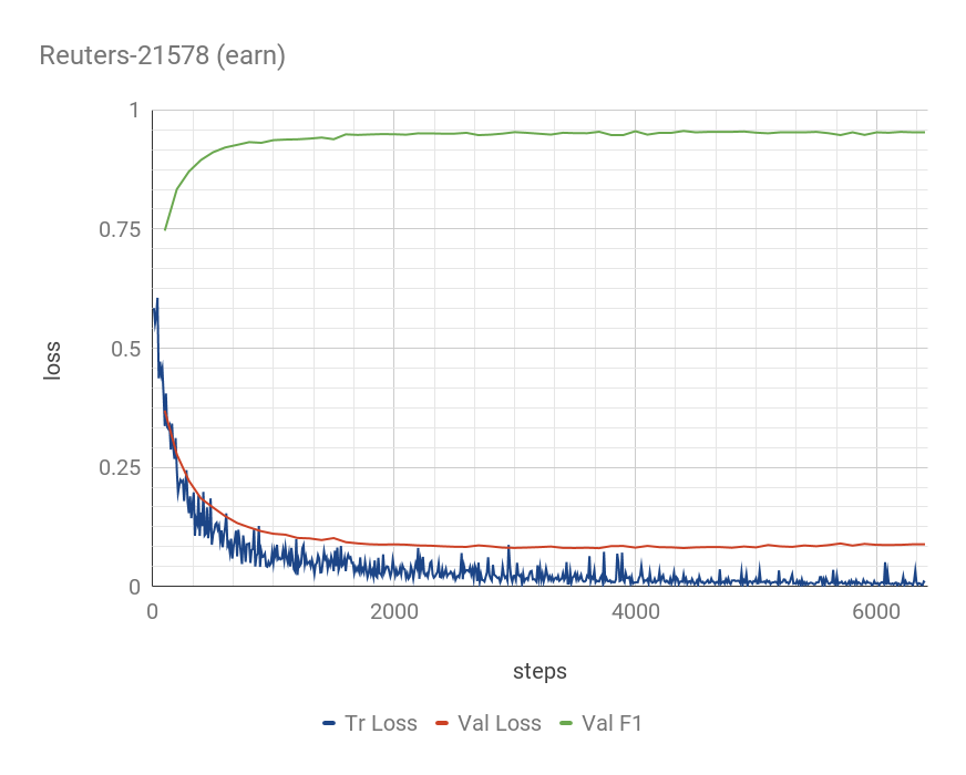
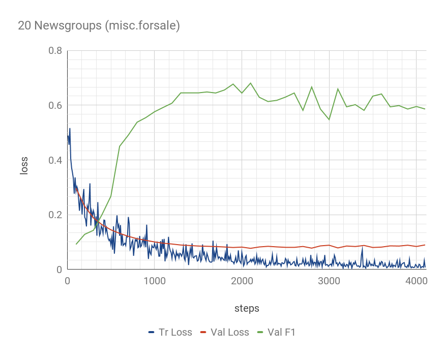
5.8 A Note on Convergence and Efficiency
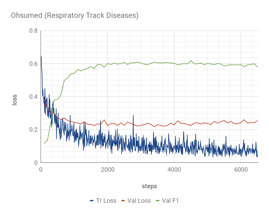
As a learning procedure, LTW is exposed to the typical problems that arise in the realm of optimization methods. Notwithstanding this, we observe that the different models converge smoothly to good solutions in the parameter space (as demonstrated in classification performance), with low tendency to overfit. Figure 5 shows the convergence trends for LTW-L-I for the same sample classes used in Figure 4 (we observe that all the LTW variants we propose and all the classes from our three datasets exhibit a qualitatively similar behaviour in terms of convergence). Note that, in all cases, an early termination is activated before the maximum number of iterations is reached. That is, irrespectively of the ongoing reduction in training loss, the process terminates when no further improvement is recorded in a validation set. Apart from preventing overfitting, this mechanism speeds up the optimization time noticeably.
Although execution times depend largely on the implementation and the hardware, it is fair to note that LTW approaches are slower than UTW methods and most STW methods (with the exception of CCA). For example, on the same machine161616All timings were recorded on the same machine, equipped with a 12-core processor Intel Core i7-4930K at 3.40GHz with 32 GB of RAM and an Nvidia GeForce GTX 1080, under Ubuntu 16.04 (LTS) and on average, it tales less than a second for any UTW to compute term weights for the Reuters-21578 collection, while STW requires 23 seconds and LTW requires 62 seconds. Despite the increase in execution time, it is also fair to note that this penalty is affordable, since the time bottleneck still lies on the tasks of training the classifier and optimizing the hyperparameters in the validation phase, which are run once for all. Additionally, given the continuous improvements and massive parallelization of new GPUs, it would not be surprising to see this difference in performance to considerably soften in the near future.171717FastText is peculiar in this respect, since the document representation phase and the classifier training phase are undertaken simultaneously. On average, it tales 10 seconds to process Reuters-21578, 31 seconds to process Ohsumed (we use 100 epochs for both), and 79 seconds to process 20Newsgroups (500 epochs). CCA is by far the slowest method among those considered in our experiments: although the execution time in any genetic algorithm depends on many variables (number of iterations, population size, etc.), on average it takes no less than 1,005 seconds for our (highly parallelized) implementation of CCA to evolve the weighting function for each class of Reuters-21578, 3,235 seconds for 20Newsgroups, and 3,075 seconds for Ohsumed.
6 Would Learning the Factor also Help?
So far we have framed the LTW framework as one that learns the IDF-like component (the factor) alone, relying on a predefined and fixed function for handling the term frequency component. Despite the fact that the above is consistent with previous STW literature, it might seem legitimate to also try to learn the component. In fact, one might argue for explicitly optimizing also the factor (instead of using e.g., a predefined log-scaled function) by saying that the impact of term frequency on the importance of a feature might in principle be captured by functions different from the ones routinely used for this, e.g., by functions that are not necessarily monotonic. In this section we report on experiments we have conducted in order to ascertain whether explicitly optimizing also the factor might be beneficial.
To this aim, we have investigated a variant of the Local LTW architecture (see Figure 3(a)) in which the left branch is replaced by a component modelled by equations
| (22) | ||||
where and (for are the new parameters to be learned alongside the previously defined set of parameters and (for . In order to preserve sparsity, we force to be 0 if feature does not occur in document .
For this experiment we consider 100 hidden units in layer , which yield additional parameters, and apply a 0.2 dropout to neurons in the hidden layer. We leave the rest of the parameters untouched.
Table IV shows the results we have obtained for this variant (here denoted LTW-TF). For the sake of clarity, we only report the results for the SVM learner (all other learners displayed similar patterns), together with the percentage of relative improvement with respect to the LTW counterpart (we here choose the LTW-L-I variant) that does not optimize the component.
| Reuters-21578 | 0.586 | (-6.84%) | 0.865 | (-1.04%) |
|---|---|---|---|---|
| 20Newsgroups | 0.623 | (-1.01%) | 0.645 | (-0.70%) |
| Ohsumed | 0.639 | (-1.52%) | 0.685 | (-0.41%) |
The results show that explicitly learning the component does not bring about any advantage. Actually, doing it degrades performance (and, according to the Wilcoxon signed-rank test, this difference is statistically significant at confidence level ). This might come as a surprise, given that LTW-TF has more parameters than LTW-L-I, which means it could well have learned the log-scaled version that LTW-L-I uses if this is indeed the best choice.
So, why is LTW-TF not superior? In principle, one might think that the proposed model is inadequate, which would imply that LTW-TF is not able to learn any meaningful function. However, that this is not the case can be seen by inspecting the actual functions that the model learns, that do seem meaningful. As an example, Figure 6 plots the functions learned for the same example classes used for Figures 4 and 5, and compares them with typical functions used to instantiate the factor (all functions are normalized so as to facilitate their comparison). Indeed, the functions that the model learns seem meaningful. For example, for the Reuters-21578 example class (see Figure 6(top)) the learned function is increasing between low () to middle frequencies (), then decreases until and is 0 thereafter; this pattern is aligned with Luhn’s intuition that the most important words are characterized by intermediate frequencies while words that are too rare or too frequent should instead be attributed low importance. In the case of 20Newsgroups (see Figure 6(middle)) the learned function displays a monotonic and quasi-linear behaviour from approximately 0.5 onwards; this resembles another well-known instantiation of the factor, i.e., the function already documented in past IR literature (see, e.g., [16, 1]). Also in Ohsumed (see Figure 6(bottom)) the model seems to have found meaningful patterns, somehow resembling the logarithmic variants of the factor. We have observed similar (and analogously meaningful) patterns for the other classes too. In sum, it is clear that the degradation in performance observed in Table IV cannot be explained by the supposed inability of the branch of the LTW-TF architecture to learn meaningful functions.
Rather, our conjecture is that the increase in the number of parameters complicates the optimization procedure more than it improves the model flexibility, and that the net effect is a model more difficult to optimize.
7 Conclusions
While standard (unsupervised) term weighting approaches do not leverage the distribution of the term across the classes, supervised ones are able to exploit this information. However, the improvements that these supervised methods have shown with respect to their unsupervised variants have not been, so far, systematic. After discussing the possible causes of this, we have discussed our conjecture that a pre-defined “Holy Grail” formula for supervised term weighting, after all, may not exist. Based on this intuition we have proposed “Learning to Weight”, a framework for learning a supervised term weighting function tuned on the available training set. We have shown several instantiations of this framework to consistently outperform previously propised (unsupervised or supervised) term weighting approaches, on several standard datasets and using different learning algorithms for training classifiers. The analysis of the weighting functions that our algorithm has learned supports our hypothesis that the optimal geometrical shape of the function is dependent on the underlying data distribution.
From the point of view of the optimization processes (in particular: the architecture of the neural networks) our approach presents some novelty as well, since the part of the supervised term weighting function may be thought of as a regulariser operating on feature statistics. That is, the architecture we propose can be interpreted as a traditional feedforward network (the part and logistic regressor) which is regularised (through the part) with constant feature statistics (extracted from the matrix columns) that control the information flow of the examples (i.e., the matrix rows). In the future it may be worthwhile to experiment with such kind of regulariser outside the scope of text classification.
Directions for future work include investigating the inclusion of more elaborated statistics about the correlation between features and classes (such as, e.g., Kullback-Leibler divergence, Fisher Information, or other feature scoring functions). We also plan to test “Learning to Weight” in multiclass classification settings, i.e., by considering all classes jointly via global policies. It would also be interesting to extend the framework so as to jointly learn not only the function but also its normalisation component. Finally, we believe that “Learning to Weight” might in principle also be useful in other tasks related to text classification, such as in learning to rank or feature selection.
References
- [1] G. Salton and C. Buckley, “Term-weighting approaches in automatic text retrieval,” Information Processing and Management, vol. 24, no. 5, pp. 513–523, 1988.
- [2] G. Paltoglou and M. Thelwall, “A study of information retrieval weighting schemes for sentiment analysis,” in Proceedings of the 48th Annual Meeting of the Association for Computational Linguistics (ACL 2010), Uppsala, SE, 2010, pp. 1386–1395.
- [3] J. Zobel and A. Moffat, “Exploring the similarity space,” SIGIR Forum, vol. 32, no. 1, pp. 18–34, 1998.
- [4] S. E. Robertson and H. Zaragoza, “The probabilistic relevance framework: BM25 and beyond,” Foundations and Trends in Information Retrieval, vol. 3, no. 4, pp. 333–389, 2009.
- [5] H. P. Luhn, “A statistical approach to mechanized encoding and searching of literary information,” IBM Journal of Research and Development, vol. 1, no. 4, pp. 309–317, 1957.
- [6] K. Spärck Jones, “A statistical interpretation of term specificity and its application in retrieval,” Journal of Documentation, vol. 28, no. 1, pp. 11–21, 1972.
- [7] S. Na, “Two-stage document length normalization for information retrieval,” ACM Transactions on Information Systems, vol. 33, no. 2, pp. 8:1–8:40, 2015.
- [8] A. Singhal, C. Buckley, and M. Mitra, “Pivoted document length normalization,” in Proceedings of the 19th ACM International Conference on Research and Development in Information Retrieval (SIGIR 1996), Zürich, CH, 1996, pp. 21–29.
- [9] F. Debole and F. Sebastiani, “Supervised term weighting for automated text categorization,” in Proceedings of the 18th ACM Symposium on Applied Computing (SAC 2003), Melbourne, US, 2003, pp. 784–788.
- [10] G. H. John, R. Kohavi, and K. Pfleger, “Irrelevant features and the subset selection problem,” in Proceedings of the 11th International Conference on Machine Learning (ICML 1994), New Brunswick, US, 1994, pp. 121–129.
- [11] Y. Yang and J. O. Pedersen, “A comparative study on feature selection in text categorization,” in Proceedings of the 14th International Conference on Machine Learning (ICML 1997), Nashville, US, 1997, pp. 412–420.
- [12] I. Batal and M. Hauskrecht, “Boosting KNN text classification accuracy by using supervised term weighting schemes,” in Proceedings of the 18th ACM Conference on Information and Knowledge Management (CIKM 2009), Hong Kong, CN, 2009, pp. 2041–2044.
- [13] P. Soucy and G. W. Mineau, “Beyond TFIDF weighting for text categorization in the vector space model,” in Proceedings of the 19th International Joint Conference on Artificial Intelligence (IJCAI 2005), Edinburgh, UK, 2005, pp. 1130–1135.
- [14] M. Lan, C. L. Tan, J. Su, and Y. Lu, “Supervised and traditional term weighting methods for automatic text categorization,” IEEE Transactions on Pattern Analysis and Machine Intelligence, vol. 31, no. 4, pp. 721–735, 2009.
- [15] X. Quan, L. Wenyin, and B. Qiu, “Term weighting schemes for question categorization,” IEEE Transactions on Pattern Analysis and Machine Intelligence, vol. 33, no. 5, pp. 1009–1021, 2011.
- [16] R. Baeza-Yates and B. Ribeiro-Neto, Modern Information Retrieval, 2nd ed. Addison Wesley, 2011.
- [17] G. Salton, Ed., The SMART Retrieval System: Experiments in Automatic Document Processing. Englewood Cliffs, US: Prentice-Hall, 1971.
- [18] J. S. Whissell and C. L. Clarke, “Improving document clustering using okapi BM25 feature weighting,” Information Retrieval, vol. 14, no. 5, pp. 466–487, 2011.
- [19] F. Sebastiani, “Machine learning in automated text categorization,” ACM Computing Surveys, vol. 34, no. 1, pp. 1–47, 2002.
- [20] M. Lan, S.-Y. Sung, H.-B. Low, and C.-L. Tan, “A comparative study on term weighting schemes for text categorization,” in Proceedings of the IEEE International Joint Conference on Neural Networks (IJCNN 2005), Montreal, CA, 2005, pp. 546–551.
- [21] G. Domeniconi, G. Moro, R. Pasolini, and C. Sartori, “A study on term weighting for text categorization: A novel supervised variant of tf.idf,” in Proceedings of 4th International Conference on Data Management Technologies and Applications (DATA 2015), Colmar, FR, 2015, pp. 26–37.
- [22] M. Haddoud, A. Mokhtari, T. Lecroq, and S. Abdeddaïm, “Combining supervised term-weighting metrics for SVM text classification with extended term representation,” Knowledge and Information Systems, vol. 49, no. 3, pp. 909–931, 2016.
- [23] N. Shanavas, H. Wang, Z. Lin, and G. I. Hawe, “Supervised graph-based term weighting scheme for effective text classification,” in Proceedings of the 22nd European Conference on Artificial Intelligence (ECAI 2016), The Hague, NL, 2016, pp. 1710–1711.
- [24] D. Wang and H. Zhang, “Inverse-category-frequency based supervised term weighting schemes for text categorization,” Journal of Information Science and Engineering, vol. 29, no. 2, pp. 209–225, 2013.
- [25] H. Wu, X. Gu, and Y. Gu, “Balancing between over-weighting and under-weighting in supervised term weighting,” Information Processing and Management, vol. 53, no. 2, pp. 547–557, 2017.
- [26] Y. Kim and O. Zhang, “Credibility adjusted term frequency: A supervised term weighting scheme for sentiment analysis and text classification,” in Proceedings of the 5th Workshop on Computational Approaches to Subjectivity, Sentiment and Social Media Analysis (WASSA 2014), Baltimore, US, 2014, pp. 79–83.
- [27] T. T. Nguyen, K. Chang, and S. C. Hui, “Supervised term weighting for sentiment analysis,” in Proceedings of the 9th IEEE International Conference on Intelligence and Security Informatics (ISI 2011), Beijing, CN, 2011, pp. 89–94.
- [28] Y. LeCun, Y. Bengio, and G. Hinton, “Deep learning,” Nature, vol. 521, no. 7553, pp. 436–444, 2015.
- [29] T. Mikolov, I. Sutskever, K. Chen, G. S. Corrado, and J. Dean, “Distributed representations of words and phrases and their compositionality,” in Proceedings of the 27th Annual Conference on Neural Information Processing Systems (NIPS 2013), Lake Tahoe, US, 2013, pp. 3111–3119.
- [30] P. Bojanowski, E. Grave, A. Joulin, and T. Mikolov, “Enriching word vectors with subword information,” Transactions of the Association for Computational Linguistics, vol. 5, pp. 135–146, 2017.
- [31] E. Grave, T. Mikolov, A. Joulin, and P. Bojanowski, “Bag of tricks for efficient text classification,” in Proceedings of the 15th Conference of the European Chapter of the Association for Computational Linguistics (EACL 2017), Valencia, ES, 2017, pp. 427–431.
- [32] H. M. de Almeida, M. A. Gonçalves, M. Cristo, and P. Calado, “A combined component approach for finding collection-adapted ranking functions based on genetic programming,” in Proceedings of the 30th ACM International Conference on Research and Development in Information Retrieval (SIGIR 2007), Amsterdam, NL, 2007, pp. 399–406.
- [33] T. Fawcett, “An introduction to ROC analysis,” Pattern Recognition Letters, vol. 27, pp. 861–874, 2006.
- [34] K. Hornik, “Approximation capabilities of multilayer feedforward networks,” Neural Networks, vol. 4, no. 2, pp. 251–257, 1991.
- [35] W. Hersh, C. Buckley, T. Leone, and D. Hickman, “OHSUMED: An interactive retrieval evaluation and new large text collection for research,” in Proceedings of the 17th ACM International Conference on Research and Development in Information Retrieval (SIGIR 1994), Dublin, IE, 1994, pp. 192–201.
- [36] T. Joachims, “Text categorization with support vector machines: Learning with many relevant features,” in Proceedings of the 10th European Conference on Machine Learning (ECML 1998), Chemnitz, DE, 1998, pp. 137–142.
- [37] R.-E. Fan, K.-W. Chang, C.-J. Hsieh, X.-R. Wang, and C.-J. Lin, “LIBLINEAR: A library for large linear classification,” Journal of Machine Learning Research, vol. 9, pp. 1871–1874, 2008.
- [38] J. D. Rennie, L. Shih, J. Teevan, and D. R. Karger, “Tackling the poor assumptions of Naive Bayes text classifiers,” in Proceedings of the 20th International Conference on Machine Learning (ICML 2003), Washington, US, 2003, pp. 616–623.
- [39] T. Mikolov, W.-T. Yih, and G. Zweig, “Linguistic regularities in continuous space word representations,” in Proceedings of the 2013 Conference of the North American Chapter of the Association for Computational Linguistics (NAACL 2013), Atlanta, US, 2013, pp. 746–751.
- [40] M. Abadi and other 39 authors, “Tensorflow: Large-scale machine learning on heterogeneous distributed systems,” 2016, arXiv:1603.04467.
- [41] D. Kingma and J. Ba, “Adam: A method for stochastic optimization,” arXiv preprint arXiv:1412.6980, 2014.
- [42] F. Pedregosa, G. Varoquaux, A. Gramfort, V. Michel, B. Thirion, O. Grisel, M. Blondel, P. Prettenhofer, R. Weiss, V. Dubourg, J. Vanderplas, A. Passos, D. Cournapeau, M. Brucher, M. Perrot, and E. Duchesnay, “Scikit-learn: Machine learning in Python,” Journal of Machine Learning Research, vol. 12, pp. 2825–2830, 2011.
- [43] T. Salles, M. Gonçalves, V. Rodrigues, and L. Rocha, “Broof: Exploiting out-of-bag errors, boosting and random forests for effective automated classification,” in Proceedings of the 38th ACM Conference on Research and Development in Information Retrieval (SIGIR 2015), Santiago, CL, 2015, pp. 353–362.
- [44] D. Zhang, J. Wang, X. Zhao, and X. Wang, “A Bayesian hierarchical model for comparing average F1 scores,” in Proceedings of the 15th IEEE International Conference on Data Mining (ICDM 2015), Atlantic City, US, 2015, pp. 589–598.