A Real-Time Wideband Neural Vocoder at 1.6 kb/s Using LPCNet

Abstract

Neural speech synthesis algorithms are a promising new approach for coding speech at very low bitrate. They have so far demonstrated quality that far exceeds traditional vocoders, at the cost of very high complexity. In this work, we present a low-bitrate neural vocoder based on the LPCNet model. The use of linear prediction and sparse recurrent networks makes it possible to achieve real-time operation on general-purpose hardware. We demonstrate that LPCNet operating at 1.6 kb/s achieves significantly higher quality than MELP and that uncompressed LPCNet can exceed the quality of a waveform codec operating at low bitrate. This opens the way for new codec designs based on neural synthesis models.

Index Terms: neural speech synthesis, wideband coding, vocoder, LPCNet, WaveRNN

1 Introduction

Very low bitrate parametric codecs have existed for a long time [1, 2], but their quality has always been severely limited. While they are efficient at modeling the spectral envelope (vocal tract response) of the speech using linear prediction, no such simple model exists for the excitation. Despite some advances [3, 4, 5], modeling the excitation signal has remained a challenge. For that reason, parametric codecs are rarely used above 3 kb/s.

Neural speech synthesis algorithms such as Wavenet [6] and SampleRNN [7] have recently made it possible to synthesize high quality speech. They have also been used in [8, 9] (WaveNet) and [10] (SampleRNN) to synthesize high-quality speech from coded features, with a complexity in the order of 100 GFLOPS. This typically makes it impossible to use those algorithms in real time without high-end hardware (if at all). In this work, we focus on simpler models, that can be implemented on general-purpose hardware and mobile devices for real-time communication, and that work for any speaker, in any language. Moreover, we target the very low bitrate of 1.6 kb/s, which is beyond the reach of conventional waveform speech coders.

To reduce computational complexity, WaveRNN [11] uses a sparse recurrent neural network (RNN). Other models use linear prediction to remove the burden of spectral envelope modeling from the neural synthesis network [12, 13, 14]. That includes our previous LPCNet work [12] (summarized in Section 2), which augments WaveRNN with linear prediction to achieve low complexity speaker-independent speech synthesis.

We now address quantization of the LPCNet features to achieve low-bitrate speech coding (Section 3). Section 4 discusses training considerations, and Section 5 presents our results. We conclude with ideas for improvement in Section 6.

2 LPCNet Overview

The WaveRNN model [11] is based on a sparse gated recurrent unit (GRU) [15] layer. At time $t$, it uses the previous audio sample $s_{t-1}$, as well as frame conditioning parameters to generates a discrete probability distribution $P\left(s_{t}\right)$ from which the output $s_{t}$ is sampled. LPCNet [12] improves on WaveRNN by adding linear prediction, as shown in Fig. 1. It is divided in two parts: a frame rate network that computes conditioning features for each 10-ms frame, and a sample rate network that computes conditional sample probabilities. In addition to using the previously generated speech sample $s_{t-1}$, LPCNet also uses the $16^{th}$ order prediction $p_{t}=\sum_{i=1}^{16}a_{i}s_{t-i}$ and the previously generated excitation $e_{t-1}$, where $e_{t}=s_{t}-p_{t}$.

LPCNet operates on signals quantized using 256-level $\mu$-law. To avoid audible quantization noise we apply a pre-emphasis filter $E(z)=1-\alpha z^{-1}$ on the input speech (with $\alpha=0.85$) and the inverse (de-emphasis) filter on the output. This shapes the noise and makes it less perceptible. Considering that $s_{t-1}$, $p_{t}$, and $e_{t-1}$ are discrete, we can pre-compute the contribution $\mathbf{v}_{i}^{\left(\cdot,\cdot\right)}$ of each possible value to the $\mathrm{GRU_{A}}$ gates and state so that only lookups are necessary at run-time. In addition, the contribution $\mathbf{g}^{\left(\cdot\right)}$ of the frame rate network to $\mathrm{GRU_{A}}$ can be computed only once per frame. After these simplifications, only the recurrent matrices $\mathbf{W}_{\left(\cdot\right)}$ remain and the sample rate network is computed as

$$\mathbf{u}_{t}= \sigma\left(\mathbf{W}_{u}\mathbf{h}_{t-1}+\mathbf{v}_{s_{t-1}}^{\left(u,s\right)}+\mathbf{v}_{p_{t}}^{\left(u,p\right)}+\mathbf{v}_{e_{t-1}}^{\left(u,e\right)}+\mathbf{g}^{\left(u\right)}\right)$$

$$\mathbf{r}_{t}= \sigma\left(\mathbf{W}_{r}\mathbf{h}_{t-1}+\mathbf{v}_{s_{t-1}}^{\left(r,s\right)}+\mathbf{v}_{p_{t}}^{\left(r,p\right)}+\mathbf{v}_{e_{t-1}}^{\left(r,e\right)}+\mathbf{g}^{\left(r\right)}\right)$$ (1)

$$\widetilde{\mathbf{h}}_{t}= \tau\left(\mathbf{r}_{t}\circ\left(\mathbf{W}_{h}\mathbf{h}_{t-1}\right)+\mathbf{v}_{s_{t-1}}^{\left(h,s\right)}+\mathbf{v}_{p_{t}}^{\left(h,p\right)}+\mathbf{v}_{e_{t-1}}^{\left(h,e\right)}+\mathbf{g}^{\left(h\right)}\right)$$

$$\mathbf{h}_{t}= \mathbf{u}_{t}\circ\mathbf{h}_{t-1}+\left(1-\mathbf{u}_{t}\right)\circ\widetilde{\mathbf{h}}_{t}$$

$$P\left(e_{t}\right) =\mathrm{softmax}\left(\mathrm{dual\_fc}\left(\mathrm{GRU_{B}}\left(\mathbf{h}_{t}\right)\right)\right)\,,$$

where $\sigma\left(x\right)$ is the sigmoid function, $\tau\left(x\right)$ is the hyperbolic tangent, $\circ$ denotes an element-wise vector multiply, and $\mathrm{GRU_{B}}\left(\cdot\right)$ is a regular (non-sparse) GRU. The dual fully-connected (dual_fc) layer is defined as

$$\mathrm{dual\_fc}(\mathbf{x})=\mathbf{a}_{1}\circ\tau\left(\mathbf{W}_{1}\mathbf{x}\right)+\mathbf{a}_{2}\circ\tau\left(\mathbf{W}_{2}\mathbf{x}\right)\,,$$ (2)

where $\mathbf{W}_{1}$ and $\mathbf{W}_{2}$ are weight matrices and $\mathbf{a}_{1}$ and $\mathbf{a}_{2}$ are scaling vectors.

Throughout this paper, biases are omitted for clarity. The synthesized excitation sample $e_{t}$ is obtained by sampling from the probability distribution $P\left(e_{t}\right)$ after lowering the temperature of voiced frames as described in eq. (7) of [12]. As a way of reducing the complexity, $\mathrm{GRU_{A}}$ uses sparse recurrent matrices with non-zero blocks of size 16x1 to ensure efficient vectorization. Because the hidden state update is more important than the reset and update gates, we keep 20% of the weights in $\mathbf{W}_{h}$, but only 5% of those in $\mathbf{W}_{r}$ and $\mathbf{W}_{u}$, for an average of 10%.

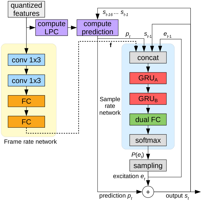
Figure 1: Overview of the LPCNet model. The frame rate network (yellow) operates on 10-ms frames and its output is held constant through each frame for the sample rate network (blue). The compute prediction block applies linear prediction to predict the sample at time $t$ from the previous samples. Conversions between $\mu$-law and linear are omitted for clarity. The de-emphasis filter is applied to the output $s_{t}$.

3 Features and Quantization

LPCNet is designed to operate with 10-ms frames. Each frame includes 18 cepstral coefficients, a pitch period (between 16 and 256 samples), and a pitch correlation (between 0 and 1). To achieve a low bitrate, we use 40-ms packets, each representing 4 LPCNet frames. Each packet is coded with 64 bits, allocated as shown in Table 1, for a total bitrate of 1.6 kb/s (constant bitrate). The prediction coefficients are computed using the quantized cepstrum.

In addition to the packet size of 40 ms, LPCNet has a synthesis look-ahead of 25 ms: 20 ms for the two 1x3 convolutional layers in the frame rate network and 5 ms for the overlap in the analysis window (see Section 3.2). The total algorithmic delay of the codec is thus 65 ms. Because the complexity of the frame-level processing is negligible compared to that of the sample rate network, no significant delay is added by the computation time (unlike traditional codecs where up to one frame delay can be added if the codec takes 100% CPU).

3.1 Pitch

Extracting the correct pitch (without period doubling or halving) is very important for a vocoder since no residual is coded to make up for prediction errors. During development, we have observed that unlike traditional vocoders, LPCNet has some ability to compensate for incorrect pitch values, but only up to a point. Moreover, that ability is reduced when the cepstrum is quantized.

The pitch search operates on the excitation signal. Maximizing the correlation over an entire 40-ms packet does not produce good results because the pitch can vary within that time. Instead, we divide each packet in 5-ms sub-frames, and find the set of pitch lags $\tau_{i}$ that maximize

$$J=\sum_{i}\left[w_{i}r\left(\tau_{i}\right)-\Theta\left(\tau_{i}-\tau_{i-1}\right)\right]\,,$$ (3)

where $w_{i}$ is the ratio of the sub-frame $i$ energy over the average energy of the 40-ms packet, $\Theta\left(\Delta\tau\right)$ is a transition penalty defined as

$$\Theta\left(\Delta\tau\right)=\begin{cases}0.02\left(\Delta\tau\right)^{2}&\mathrm{if}\,\left|\Delta\tau\right|\leq 4\\ 6&\mathrm{otherwise}\end{cases}\,,$$ (4)

and $r\left(\tau\right)$ is a modified pitch correlation [16]

$$r\left(\tau\right)=\frac{2\sum_{n}e\left(n\right)e\left(n-\tau\right)}{\sum_{n}e^{2}\left(n\right)+\sum_{n}e^{2}\left(n-\tau\right)}\,.$$ (5)

The optimal path can be computed efficiently using dynamic programming with a Viterbi search. Since the entire audio is not available at once, the values of $J$ in the forward pass are updated normally for every sub-frame but the Viterbi backtrack pass is computed once per 40-ms packet, over all 8 sub-frames. While that does not guarantee finding the global optimal path, it ensures a consistent pitch over the duration of the packet, which is important for quantization.

The pitch is allowed to vary between 62.5 Hz and 500 Hz. The average pitch over the packet is encoded on a logarithmic scale using 6 bits, resulting in quantization intervals of 0.57 semitones.

A linear pitch modulation parameter allows up to 16% variation (2.5 semitones) between the first and last sub-frame. It is encoded with 3 bits representing a $\left[-3,3\right]$ range with two different codes for 0 (constant modulation), one of which signaling that the pitch correlation is less than 0.3 (the modulation is zero when the pitch correlation is too small). Two extra bits refine the value of the pitch correlation within the remaining range (either $\left[0,\,0.3\right]$ or $\left[0.3,\,1\right]$).

Table 1: Bit allocation for a 40-ms frame.

Parameter	Bits
Pitch period	6
Pitch modulation	3
Pitch correlation	2
Energy (C0)	7
Cepstrum VQ (40 ms)	30
Cepstrum delta (20 ms)	13
Cepstrum interpolation (10 ms)	3
Total	64

3.2 Cepstrum

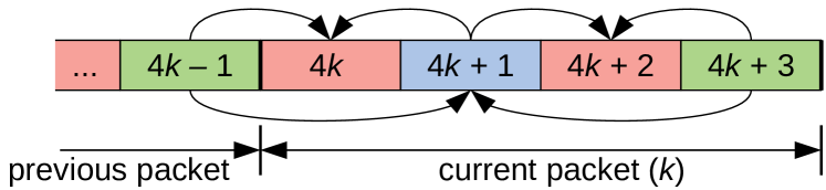
Figure 2: Prediction and quantization of the cepstrum for packet $k$. Vectors in green are quantized independently, vectors in blue are quantized with prediction, and vectors in red use prediction with no residual quantization. Prediction is shown by the arrows.

The spectral feature analysis operates on 20-ms windows with a 10-ms frame offset (50% overlap). The cepstrum is computed from 18 Bark-spaced bands following the same layout as [17]. Because we pack 4 cepstral vectors in each packet, we wish to minimize redundancy within a packet while limiting dependencies across packets to reduce the effect of packet loss. For those reasons, we use a prediction scheme (Fig. 2) inspired by video codec B-frames [18], limiting the error propagation in case of packet loss to a worst case of 30 ms.

Let packet $k$ include cepstral vectors $\mathbf{c}_{4k}$ to $\mathbf{c}_{4k+3}$. We start by coding the first component (C0) of $\mathbf{c}_{4k+3}$ independently, with a uniform 7-bit scalar quantizer (0.83 dB resolution). We then code the remaining component of $\mathbf{c}_{4k+3}$ independently using a 3-stage codebook with 17 dimensions and 10 bits for each stage. An M-best (survivor) search helps reduce the quantization error, but is not strictly necessary. From there, vector $\mathbf{c}_{4k+1}$ is predictively coded using both $\mathbf{c}_{4k-1}$ (independently coded in the previous packet) and $\mathbf{c}_{4k+3}$. We use a single bit to signal if the prediction is the average ($\frac{\mathbf{c}_{4k-1}+\mathbf{c}_{4k+3}}{2}$), or two bits if the prediction is either of $\mathbf{c}_{4k-1}$ or $\mathbf{c}_{4k+3}$. The 18-dimensional prediction residual is then coded with a 11-bit + sign codebook for the average predictor or with an 10-bit + sign codebook if not, for a total of 13 bits for $\mathbf{c}_{4k+1}$. Although the average predictor is the most useful, including the single-vector predictors improves the quantization of transients/onsets.

Because there is insufficient bitrate to adequately code $\mathbf{c}_{4k}$ and $\mathbf{c}_{4k+2}$, we only use a prediction from their neighbors. Vector $\mathbf{c}_{4k}$ is predicted from its neighbors $\mathbf{c}_{4k-1}$ and $\mathbf{c}_{4k+1}$, whereas $\mathbf{c}_{4k+2}$ is predicted from $\mathbf{c}_{4k+1}$ and $\mathbf{c}_{4k+3}$. Since there are 3 options for each vector, we have 9 possible combinations. By eliminating the least useful combination (forcing both equal to $\mathbf{c}_{4k+1}$), we can code the remaining ones with 3 bits.

4 Training

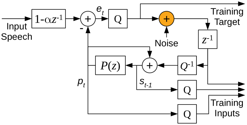
Figure 3: Noise injection during the training procedure, with $Q$ denoting $\mu$-law quantization and $Q^{-1}$ denoting conversion from $\mu$-law to linear. The prediction filter filter is given by $P\left(z\right)=\sum_{i=1}^{M}a_{i}z^{-k}$. The target excitation is computed as the difference between the clean, unquantized input and the noisy prediction. Note that the noise is added in the $\mu$-law domain so that its power follows that of the real excitation signal.

When decoding speech, the sample rate network operates on the synthesized speech rather than on the ground-truth clean speech. That mismatch between training and inference can increase the speech distortion, in turn increasing the mismatch. To make the network more robust to the mismatch, we add noise to the training data, as originally suggested in [19]. As an improvement over our previous work [12], Laplace-distributed noise is added to the excitation inside the prediction loop, making the signal and excitation noise consistent with each other, as shown in Fig. 3.

As a way of making the model more robust to input variations, we use data augmentation on the training database. The speech level is varied over a 40 dB range and the frequency response is varied according to eq. (7) in [17].

Training is first performed with unquantized features. When training a model for quantized features, we start with a model trained on unquantized features, and apply domain adaptation to quantized features. We have observed that better results are obtained when only the frame rate network is adapted, with the sample rate network weights left unchanged. In addition to the slightly better quality, this has the advantage of faster training for new quantizers and also smaller storage if different quantized models are needed.

5 Evaluation

The source code for this work is available under a BSD license at https://github.com/mozilla/LPCNet/. The evaluation in this section is based on commit 6fda6b7.

5.1 Complexity and Implementation

The number of weights in the sample rate network is approximately

$$W=3dN_{A}^{2}+3N_{B}\left(N_{A}+N_{B}\right)+2N_{B}Q\,,$$ (6)

where $N_{A}$ and $N_{B}=16$ are the sizes of the two GRUs, $d$ is the density of the sparse GRU, and $Q=256$ is the number of $\mu$-law levels. Based on the subjective results in [12], we consider $N_{A}=384$ with $d=10\%$ (122 dense equivalent units) to provide a good compromise between quality and complexity. This results in $W=71600\,\mathrm{weights}$, which fits in the L2 or L3 cache of most modern CPUs. Considering that each weight is used once per sample for a multiply-add, the resulting complexity is 2.3 GFLOPS. The activation functions are based on a vectorized exponential approximation and contribute 0.6 GFLOPS to the complexity, for a total of 3 GFLOPS when counting the remaining operations.

A C implementation of the decoder (with AVX2/FMA intrinsics) requires 20% of a 2.4 GHz Intel Broadwell core for real-time decoding (5x faster than real-time). According to our analysis, the main performance bottleneck is the L2 cache bandwidth required for the matrix-vector products. On ARMv8 (with Neon intrinsics), real-time decoding on a 2.5 GHz Snapdragon 845 (Google Pixel 3) requires 68% of one core (1.47x real-time). On the more recent 2.84 GHz Snapdragon 855 (Samsung Galaxy S10), real-time decoding requires only 31% of one core (3.2x real-time).

As a comparison, we estimate the complexity of the SampleRNN neural codec described in [10] to be around 100 GFLOPS – mostly from the MLP with two hiddens layers and 1024 units per layer. The complexity of the WaveNet-based codec in [8] significantly exceeds 100 GFLOPS. For speaker-dependent text-to-speech (TTS) – which typically allows smaller models – real-time synthesis was achieved by [20] (WaveNet) and [11] (WaveRNN) when using multiple CPU cores.

The total complexity of the proposed encoder is around 30 MFLOPS (0.03 GFLOPS), mostly from the 5-best VQ search (14 MFLOPS) and the undecimated 16 kHz pitch search (8 MFLOPS). Although the encoder complexity could be significantly reduced, it is already only 1% of the decoder complexity.

5.2 Experimental Setup

The model is trained using 4 hours of speech from the NTT Multi-Lingual Speech Database for Telephonometry (21 languages), from which we excluded all samples from the speakers used in testing. From the original data, we generate 14 hours of augmented speech data as described in Section 4. The unquantized network was trained for 120 epochs (625k updates), with a batch size size of 64, each sequence consisting of 2400 samples (15 frames). Training was performed on an Nvidia GPU with Keras/Tensorflow using the CuDNN GRU implementation and the AMSGrad [21] optimization method (Adam variant) with a step size $\alpha=\frac{\alpha_{0}}{1+\delta\cdot b}$ where $\alpha_{0}=0.001$, $\delta=5\times 10^{-5}$, and $b$ is the batch number. For model adaptation with quantized features, we used 40 epochs (208k updates) with $\alpha_{0}=0.0001$, $\delta=0$.

5.3 Quality

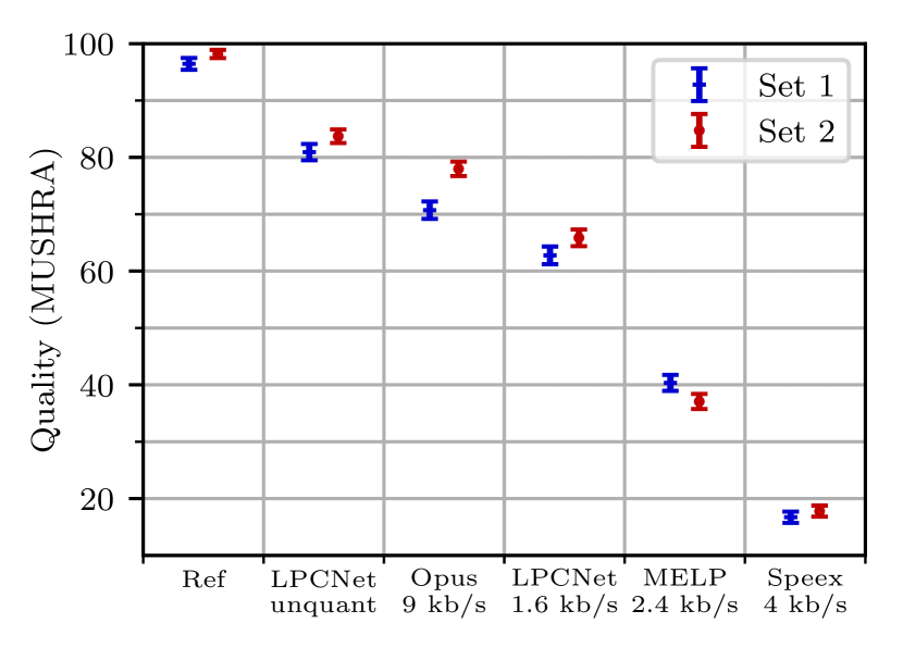
Figure 4: Subjective quality (MUSHRA) results for both listening tests. Set 1 is taken from the NTT database, while Set 2 consists of Opus testvector samples.

We conducted a subjective listening test with a MUSHRA-inspired methodology [22] to evaluate the quality of the proposed 1.6 kb/s neural vocoder. As an upper bound on the quality achievable with LPCNet at the target complexity (higher quality is achievable with a larger model), we include LPCNet operating on unquantized features. We also compare with Opus [23] wideband (SILK mode) operating at 9 kb/s VBR and with the narrowband MELP [4] vocoder. As low anchor, we use Speex [24] operating as a 4 kb/s wideband vocoder (wideband quality 0).

In a first test (Set 1), we used 8 samples from 2 male and 2 female speakers. The samples are part of the NTT database used for training, but all samples from the selected speakers for the test were excluded from the training set. As reported in [10], mismatches between the training and testing database can cause a significant difference in the output quality. We measure that impact in a second test (Set 2) on the same model, with 8 samples (one male and one female speaker) from the sample set used to create the Opus testvectors. Each test included 100 listeners.

The results in Fig. 4 show that 1.6 kb/s LPCNet clearly outperforms the MELP vocoder, making it a viable choice for very low bitrates. The fact that LPCNet with unquantized features achieves slightly higher quality than Opus at 9 kb/s suggests that LPCNet at bitrates around 2-6 kb/s may be able to compete with waveform coders below 10 kb/s. The test with samples outside the NTT database shows that the LPCNet model generalizes to other recording conditions.

Since the LPCNet model was trained on 21 languages, it is expected to also work in those languages. While we only tested on English, informal listening indicates that the quality obtained on French, Spanish, and Swedish is comparable to that on English.

A subset of the samples from the listening test is available at https://people.xiph.org/~jm/demo/lpcnet_codec/.

6 Conclusions

We have demonstrated a 1.6 kb/s neural vocoder based on the LPCNet model that can be used for real-time communication on a mobile device. The quality obtained exceeds what is achievable with existing low-bitrate vocoders such as MELP. Although other work has demonstrated similar or higher speech quality at similar bitrates [8, 9, 10], we believe this is the first neural vocoder that can operate in real-time on general-purpose hardware and mobile devices. We have so far focused on clean, non-reverberant speech. More work is needed for testing and improving the robustness to noise and reverberation.

Considering that uncompressed LPCNet is able to achieve higher quality than 9 kb/s Opus, we believe it is worth exploring higher LPCNet bitrates in the 2-6 kb/s range. Moreover, in the case of a waveform codec like Opus operating at very low bitrate (< 8kb/s) it should be possible to directly use the encoded LSPs to synthesize a higher quality output than the standard provides. In addition, using the encoded excitation as an extra input to LPCNet may help further reducing artifacts, turning LPCNet into a neural post-filter that can significantly improve the quality of any existing low-bitrate waveform codec.

7 Acknowledgements

We thank David Rowe for his feedback and suggestions, as well as for implementing some of the Neon optimizations.

References

- [1] B. S. Atal and S. L. Hanauer, “Speech analysis and synthesis by linear prediction of the speech wave,” The journal of the acoustical society of America, vol. 50, no. 2B, pp. 637–655, 1971.
- [2] J. Markel and A. Gray, “A linear prediction vocoder simulation based upon the autocorrelation method,” IEEE Transactions on Acoustics, Speech, and Signal Processing, vol. 22, no. 2, pp. 124–134, 1974.
- [3] D. Griffin and J. Lim, “A new model-based speech analysis/synthesis system,” in Proc. International Conference on Acoustics, Speech, and Signal Processing (ICASSP), vol. 10, 1985, pp. 513–516.
- [4] A. McCree, K. Truong, E. B. George, T. P. Barnwell, and V. Viswanathan, “A 2.4 kbit/s MELP coder candidate for the new US federal standard,” in Proc. International Conference on Acoustics, Speech, and Signal Processing (ICASSP), vol. 1, 1996, pp. 200–203.
- [5] D. Rowe, “Techniques for harmonic sinusoidal coding,” Ph.D. dissertation, School of Physics and Electronic Systems Engineering, July 1997.
- [6] A. van den Oord, S. Dieleman, H. Zen, K. Simonyan, O. Vinyals, A. Graves, N. Kalchbrenner, A. Senior, and K. Kavukcuoglu, “WaveNet: A generative model for raw audio,” arXiv:1609.03499, 2016.
- [7] S. Mehri, K. Kumar, I. Gulrajani, R. Kumar, S. Jain, J. Sotelo, A. Courville, and Y. Bengio, “SampleRNN: An unconditional end-to-end neural audio generation model,” arXiv:1612.07837, 2016.
- [8] W. B. Kleijn, F. S. Lim, A. Luebs, J. Skoglund, F. Stimberg, Q. Wang, and T. C. Walters, “WaveNet based low rate speech coding,” in Proc. International Conference on Acoustics, Speech, and Signal Processing (ICASSP), 2018, pp. 676–680.
- [9] C. Garbacea, A. van den Oord, Y. Li, F. Lim, A. Luebs, O. Vinyals, and T. Walters, “Low bit-rate speech coding with VQ-VAE and a WaveNet decoder,” in Proc. International Conference on Acoustics, Speech, and Signal Processing (ICASSP), 2019.
- [10] J. Klejsa, P. Hedelin, C. Zhou, R. Fejgin, and L. Villemoes, “High-quality speech coding with SampleRNN,” arXiv preprint arXiv:1811.03021, 2018.
- [11] N. Kalchbrenner, E. Elsen, K. Simonyan, S. Noury, N. Casagrande, E. Lockhart, F. Stimberg, A. van den Oord, S. Dieleman, and K. Kavukcuoglu, “Efficient neural audio synthesis,” arXiv:1802.08435, 2018.
- [12] J.-M. Valin and J. Skoglund, “LPCNet: Improving neural speech synthesis through linear prediction,” in Proc. International Conference on Acoustics, Speech, and Signal Processing (ICASSP). arXiv:1810.11846, 2019.
- [13] L. Juvela, V. Tsiaras, B. Bollepalli, M. Airaksinen, J. Yamagishi, and P. Alku, “Speaker-independent raw waveform model for glottal excitation,” in Proc. Interspeech, 2018, pp. 2012–2016.
- [14] X. Wang, S. Takaki, and J. Yamagishi, “Neural source-filter-based waveform model for statistical parametric speech synthesis,” in Proc. International Conference on Acoustics, Speech, and Signal Processing (ICASSP), 2019, arXiv:1810.11946.
- [15] K. Cho, B. van Merriënboer, D. Bahdanau, and Y. Bengio, “On the properties of neural machine translation: Encoder-decoder approaches,” in Proc. Eighth Workshop on Syntax, Semantics and Structure in Statistical Translation (SSST-8), 2014, arXiv:1409.1259.
- [16] K. Vos, K. V. Sørensen, S. S. Jensen, and J.-M. Valin, “Voice coding with Opus,” in Proc. 135th Convention of the Audio Engineering Society, 2013.
- [17] J.-M. Valin, “A hybrid DSP/deep learning approach to real-time full-band speech enhancement,” in Proc. Multimedia Signal Processing Workshop (MMSP), 2018, arXiv:1709.08243.
- [18] “Coding of moving pictures and associated audio for digital storage media at up to about 1,5 Mbit/s – part 2: Video,” ISO/IEC, Standard, Aug. 1993.
- [19] Z. Jin, A. Finkelstein, G. J. Mysore, and J. Lu, “FFTNet: A real-time speaker-dependent neural vocoder,” in Proc. International Conference on Acoustics, Speech, and Signal Processing (ICASSP), 2018, pp. 2251–2255.
- [20] S. Ö. Arik, M. Chrzanowski, A. Coates, G. Diamos, A. Gibiansky, Y. Kang, X. Li, J. Miller, A. Ng, J. Raiman, S. Sengupta, and M. Shoeybi, “Deep voice: Real-time neural text-to-speech,” in Proc. 34th International Conference on Machine Learning, vol. 70, 2017, pp. 195–204, arXiv:1702.07825.
- [21] S. J. Reddi, S. Kale, and S. Kumar, “On the convergence of Adam and beyond,” in Proc. ICLR, 2018.
- [22] ITU-R, Recommendation BS.1534-1: Method for the subjective assessment of intermediate quality level of coding systems, International Telecommunications Union, 2001.
- [23] J.-M. Valin, K. Vos, and T. B. Terriberry, “Definition of the Opus Audio Codec,” RFC 6716, Internet Engineering Task Force, Sep. 2012, https://tools.ietf.org/html/rfc6716.
- [24] J.-M. Valin, “The Speex codec manual,” Xiph.Org Foundation, 2007.