Ionization equation of state for the dusty plasma including the effect of ion–atom collisions

Abstract

The ionization equation of state (IEOS) for a cloud of the dust particles in the low-pressure gas discharge under microgravity conditions is proposed. IEOS relates pairs of the parameters specific for the charged components of dusty plasma. It is based on the modified collision enhance collection model adapted for the Wigner–Seitz cell model of the dust cloud. This model takes into account the effect of ion–atom collisions on the ion current to the dust particles and assumes that the screening length for the ion–particle interaction is of the same order of magnitude as the radius of the Wigner–Seitz cell. Included effect leads to a noticeable decrease of the particle charge as compared to the previously developed IEOS based on the orbital motion limited model. Assuming that the Havnes parameter of the dusty plasma is moderate one can reproduce the dust particle number density measured in experiments and, in particular, its dependence on the gas pressure. Although IEOS includes no fitting parameters, it can ensure a satisfactory precision in a wide range of dusty plasma parameters. Based on the developed IEOS, the threshold relation between the dusty plasma parameters for onset of the lane formation in binary dusty plasmas is deduced.

I INTRODUCTION

Low-temperature plasmas that contain dust particles typically in the range from $0.01$ to $1000\,\mu{\mbox{m}}$ are termed dusty (or complex) plasmas Fortov and Morfill (2010); Chu and Lin (1994); Thomas et al. (1994); Vladimirov et al. (2005); Fortov et al. (2005); Bonitz et al. (2010). Laboratory dusty plasmas are generated to study fundamental processes in the strong coupling regime on the kinetic level by the observation of individual microparticles. Due to the high electron mobility, particles acquire a considerable negative electric charge. Because of the Coulomb repulsion, they can form extended clouds. In the ground-based experiments, gravity is one of the crucial forces that define the properties of a dust cloud. Under microgravity conditions, e.g., on the International Space Station (ISS) Morfill et al. (2006); Schwabe et al. (2008); Morfill et al. (1999); Khrapak et al. (2011); Thomas et al. (2008); Jiang et al. (2009); Schwabe et al. (2011) or in parabolic flights Morfill et al. (2006); Caliebe et al. (2011); Piel et al. (2008); Menzel et al. (2011); Arp et al. (2011), the particles can form almost homogenous three-dimensional clouds in the bulk of the low-pressure gas discharge. In addition, due to the large particle charge, the Coulomb coupling parameter of the particle subsystem is great, so that such subsystem can form an analog of condensed state of matter, i.e., three-dimensional liquid or solid.

One of the basic objectives in this field is the investigations of correlations between the governing parameters of dusty plasmas, in particular, the spatial distribution of the local particle number density in a stationary dust cloud $n_{d}$ under different conditions of the gas discharge. Thus, the dust distribution under the conditions of PKE (plasma crystal experiment) chamber was investigated numerically Land and Goedheer (2006); equation of state for 2D liquid dusty plasmas was obtained in Feng et al. (2016); the dust distribution in the sheath under the conditions of PK-3 Plus chamber is studied in Pustylnik et al. (2017). In the works Zhukhovitskii et al. (2014, 2015a); Zhukhovitskii (2017), the particle distribution in a quasi-homogeneous region of the dust cloud apart from the void was modeled by construction of the ionization equation of state (IEOS). IEOS is a relation between a pair of the parameters specific for the charged components of complex plasma containing a cloud of the dust particles. Such parameters are the electron, the ion, and the particle number density, and the particle potential (related to its charge). A complete set of IEOS’s makes it possible to calculate all plasma state parameters provided that a single one is known. This makes IEOS similar to the common equation of state. The IEOS proposed in Zhukhovitskii et al. (2014, 2015a); Zhukhovitskii (2017) employs the balance equation for the main forces acting on a dust particle, the quasineutrality equation, and the particle charge equation. The latter is based on the orbital motion limited approximation Allen (1992) (OML), which was shown to underestimate substantially the ion flux toward the particle due to disregard of the ion–atom collisions Khrapak et al. (2012). This leads to overestimation of the particle charge and, correspondingly, to underestimation of $n_{d}$ Zhukhovitskii et al. (2014, 2015a); Zhukhovitskii (2017) as compared to the experiment. In addition, the estimated electron and ion number densities seem to be overestimated by more than an order of magnitude. The dependence of $n_{d}$ on the gas pressure observed in experiment is not reproduced by such IEOS, even if the dependence of the ion mean free path on the local particle number density is properly taken into account Zhukhovitskii (2017).

To modify our approach, we adopt the expression for the ion flux Khrapak et al. (2012), which was obtained for the case of a solitary particle in plasma, and change it for the case of a dust cloud. We show that a relevant model for the cloud is the Wigner–Seitz cell model, in which the screening length is of the same order of magnitude as the cell radius. With this screening length, one can obtain a correct expression for the ion flux to the particle and derive the particle charge equation. In the modification of IEOS proposed in this work, we use this expression instead of that based on the OML approach Zhukhovitskii (2017). The IEOS obtained in this study makes it possible to attain a good correlation between the magnitudes of all plasma parameters. In particular, it ensures a correct dependence of $n_{d}$ on the gas pressure with due regard for the dependence of the electron number density on the pressure. At the same time, this IEOS is free from fitting parameters. Nevertheless, it is valid in a wide range of dusty plasma parameters and can ensure a sufficient precision. In particular, this provides an interpretation for the decreasing dependence of $n_{d}$ on the pressure observed in the experiment Khrapak et al. (2012).

We use this new modification of IEOS to estimate the threshold relation between plasma parameters corresponding to the onset of lane formation in the binary complex plasmas observed in experiments Sütterlin et al. (2009); Morfill et al. (2012); Khrapak et al. (2016). This effect takes place if small particles are injected in a stationary cloud of large particles. Under the experimental conditions, the latter is typically a dust crystal. We assume that the lane formation is a manifestation of the crystal spallation entailed by the injection of small particles. Hence, the work of the driving force acting on the small particles must be greater than the work against the pressure of the particles that form a dust cloud. We calculate the driving force in the same way as in Zhukhovitskii (2017), however, we apply the new modification of IEOS to attain a correlation with the magnitudes of experimental parameters.

Proposed IEOS is significant for both understanding the properties of dusty plasmas and planning the future experiments. Thus, based on a standard simulation of the discharge without particles and the developed IEOS, one can estimate the parameters of complex plasma for the Ekoplasma project, which is a Russian–German cooperation building the future laboratory for the investigation of complex plasmas under microgravity conditions on the ISS Knapek et al. (2018). Such calculations will enable optimization of the conditions of forthcoming experiments.

The paper is organized as follows. In Sec. II, the screening length for a dense 3D cloud of particles in a low-pressure discharge plasma is estimated on the basis of the Wigner–Seitz cell model. In Sec. III, the effect of the ion–atom collisions on the ion current to the particle is estimated for the treated system, and the equation defining the particle charge is derived. The IEOS taking into account this effect is obtained and analyzed in Sec. IV. In Sec. V, the calculation results using obtained IEOS are compared with available experimental data. In Sec. VI, the proposed IEOS is applied to the calculation of the threshold for onset of the lane formation in binary dusty plasmas. The results of this study are summarized in Sec. VII.

II SCREENING LENGTH IN THE CELL MODEL OF A DENSE DUST CLOUD

Consider a stationary cloud of dust particles of the same radius in the low-pressure gas discharge. We will treat a “dense” cloud, in which the interparticle correlations are as strong as in the condensed state of matter. In fact, such cloud can be a model either for liquid or solid state. For this system, the Wigner–Seitz cell model will be utilized. It implies that dusty plasma is divided in spherical cells with the radius $r_{d}=(3/4\pi n_{d})^{1/3}$. Each particle finds itself in the center of a spherical cell filled with the background volume charge from the light plasma components (electrons and ions). The cell as a whole is electrically neutral, i.e., the electric field at its boundary vanishes.

Under typical conditions of the low-pressure gas discharge, the electrons are fully thermalized and they obey the Boltzmann distribution. If the particle dimensionless electric potential $\Phi=Ze^{2}/aT_{e}$, where $Z$ is the particle charge in units of the electron charge, $e$ is the elementary electric charge, $a$ is the particle radius, and $T_{e}$ is the electron temperature, is restricted by the assumed condition $\Phi<1$ then the inhomogeneity in the electron spatial distribution is only insignificantly different from a constant in the vicinity of the particle and cannot screen noticeably the particle charge. In addition, note that typically $T_{e}\sim 4\;{\mbox{eV}}$ and the electron number density $n_{e}\sim 3\times 10^{8}{\kern 1.0pt}{\mbox{cm}}^{-3}$, which means that the electron Debye screening length $r_{De}=(T_{e}/4\pi n_{e}e^{2})^{1/2}\sim 0.1\;{\mbox{cm}}$ is sufficiently large to satisfy the condition $r_{d}\ll r_{De}$.

The ions are far from equilibrium with the particles. The spatial distribution of the ion number density in the vicinity of a particle depends on the relations between the particle radius, the ion mean free path with respect to the collisions with atoms $\lambda_{a}$, and the length of dust particle screening. In the collisionless regime for a solitary small particle in the infinite stationary plasma, OML results in the buildup of ion number density around the particle and consequent screening length close to the Debye one Fortov and Morfill (2010) $r_{Di}=(T_{i}/4\pi n_{i}e^{2})^{1/2}$, where $n_{i}$ is the average ion number density. Due to low ion temperature $T_{i}\sim 0.03\;{\mbox{eV}}$, for $n_{i}\sim n_{e}$, we obtain $r_{d}\sim r_{Di}$ for the small particles and $r_{d}\gg r_{Di}$ for the large ones. If the dust cloud is modeled by the Yukawa system then the particle electric potential is prescribed the Yukawa form. However in the Wigner–Seitz cell model, the particle potential is significantly different from the Yukawa one even for the Boltzmann ion number density distribution, albeit the particle charge can be screened (renormalized) by a thin layer around a particle. This is the case when the local Debye screening length is smaller than the particle radius Zhukhovitskii et al. (1984). In our case, this would require $n_{i}>10^{12}\,{\mbox{cm}}^{-3}$, which seems unrealistic because of the non-exponential nonequilibrium radial dependence of $n_{i}$. Apparently, one can neglect the Debye screening in the cell in the collisionless case. In the opposite case of highly collisional regime ($a\gtrsim\lambda_{a}$) in the neighborhood of a particle, $n_{i}$ is lower than its volume average (see, e.g., Zhukhovitskii et al. (2014)). This excludes any ion screening of the particle charge in this region. In the region of moderate collisions treated in this study the potential of a solitary particle is almost the Coulomb one Filippov et al. (2007), and screening is absent. Unfortunately, to the best of our knowledge, no calculation of the ion number density distribution in the Wigner–Seitz cell model is available in the literature. At the same time, it seems reasonable to treat the total charge background in the cell $e(n_{i}-n_{e})$ as a uniform one.

One can conclude that in the cell model, the particle charge screening is different from the Debye one and the ion Debye length is no appropriate scale for the system. In this model, screening is caused by the overall cell quasineutrality. Hence, the screening length must be of the order of the cell radius $r_{d}$. In what follows, we will define this length.

The distribution of electric potential in the cell $\varphi(r)$ is defined by the Poisson equation

$${1\over{r^{2}}}\displaystyle{d\over{dr}}\left({r^{2}\displaystyle{{d\varphi}\over{dr}}}\right)=4\pi e(n_{e}-n_{i}),$$ (1)

which should be solved with the boundary conditions

$$\varphi(r_{d})=\varphi^{\prime}(r_{d})=0,\quad\varphi^{\prime}(a)=\displaystyle{{Ze}\over{a^{2}}}.$$ (2)

We represent the solution in the form

$$\varphi(r)=\displaystyle{A\over r}+Br^{2}+C,$$ (3)

where $A$, $B$, and $C$ are constants, to obtain

$$\varphi(r)=-\displaystyle{{Ze}\over{r_{d}}}\displaystyle{1\over{1-(a/r_{d})^{3}}}\left({\displaystyle{{r_{d}}\over r}+\displaystyle{1\over 2}\displaystyle{{r^{2}}\over{r_{d}^{2}}}-\displaystyle{3\over 2}}\right).$$ (4)

Solution (4) is compatible with the cell quasineutrality condition

$$(n_{i}-n_{e})\left({1-\displaystyle{{a^{3}}\over{r_{d}^{3}}}}\right)-Zn_{d}=0.$$ (5)

In what follows, we will neglect the very small ratio $a^{3}/r_{d}^{3}\sim 10^{-6}$.

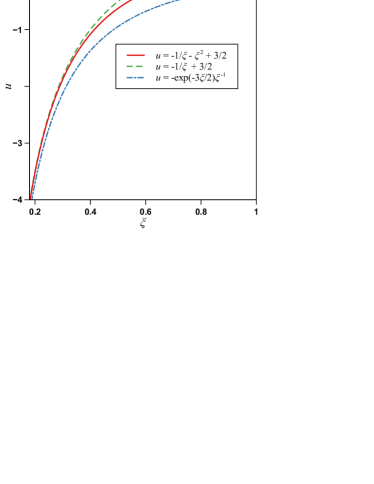
Figure 1: Particle potential in the Wigner–Seitz cell (solid line), its approximation by the shifted Coulomb potential (dashed line), and by the Yukawa potential (dash-dotted line).

The dimensionless ion potential energy in the cell $e\varphi(r)/T_{i}=(a\tau\Phi/r_{d})u(r/r_{d})$, where $\tau=T_{e}/T_{i}$, $u(\xi)=-1/\xi-\xi^{2}/2+3/2$, and $\xi=r/r_{d}$, is shown in Fig. 1. The function $u(\xi)$ can be approximated by the shifted Coulomb potential $u(\xi)\simeq-1/\xi+3/2$ if $\xi\leq 2/3$, which is the asymptotic of $u(\xi)$ at $\xi\ll 1$, and $u(\xi)\equiv 0$ if $\xi>2/3$. The same asymptotic is characteristic of the Yukawa potential $-\exp(-3\xi/2)\xi^{-1}$ (Fig. 1). Note that the Yukawa potential approximates $u(\xi)$ significantly worse than the shifted Coulomb potential. Consequently, in the cell model, the screening length can be defined as $r_{s}=(2/3)r_{d}$. For the clouds of large particles, $r_{s}$ can be considerably larger than $r_{Di}$. Since the region essential for the moment transfer from the ions to a particle is restricted by the condition $u\lesssim-1$, i.e., $r\lesssim 0.45r_{d}$, $r_{s}$ could be defined otherwise. However, it would always be $r_{s}\sim r_{d}$ for any definition.

Next, we will discuss the condition of applicability of the Wigner–Seitz cell model for the particle subsystem. Obviously, this model is appropriate for a highly correlated system of particles, in which the displacement of particles from their equilibrium positions in the crystal is much smaller than the interparticle distance. Hence, the applicability condition can be obtained in the same way as for the Wigner electron crystal, which differs from the treated system in the charge signs of the particles and the background. If the background is assumed uniform then a particle oscillates in the spherical potential well Zhukhovitskii et al. (1984) $U(\delta r)=(2\pi/3)n_{d}Z^{2}e^{2}(\delta r)^{2}$, where $\delta r$ is the deviation of a particle from the center of the cell. If $\delta r$ is equal to the rms deviation from the cell center then $U(\delta r)=M\left\langle{v^{2}}\right\rangle/2=3T_{d}/2$, where $M$ is the particle mass, $\left\langle{v^{2}}\right\rangle$ is its average velocity, and $T_{d}$ is the dust particle kinetic temperature (the Boltzmann constant is set to unity). We require the amplitude of the particle oscillations to be much smaller than the cell radius $r_{d}$, $(\delta r/r_{d})^{2}\ll 1$ to obtain the condition Zhukhovitskii et al. (2017)

$$\Gamma=3\left({\displaystyle{{r_{d}}\over{\delta r}}}\right)^{2}\gg 1,$$ (6)

where $\Gamma=Z^{2}e^{2}/r_{d}T_{d}$ is the Coulomb coupling parameter. Equation (6) is the condition of the model applicability. From (6), an important conclusion follows that the Wigner–Seitz cell model is a model of strongly coupled dusty plasma Zhukhovitskii et al. (1984). Under typical experimental conditions, $\Gamma\sim 100$, which justifies the use of this model.

As the ion–particle interaction is concerned, we note that the Wigner-Seitz cell model of dusty plasma implies that the volume screening of the particle charge by the uniform charged background is stronger than the particle screening by polarization of the background in the vicinity of a particle, as in the case of the Debye screening Zhukhovitskii et al. (1984, 2015b).

III PARTICLE CHARGE EQUATION

The stationary particle charge $Z$ is defined by the balance between the electron and ion currents to the particle. Since in the low-pressure RF discharge, the electrons are thermalized and they obey the Boltzmann distribution, the electron current is $j_{-}=-\pi a^{2}en_{e}v_{Te}\exp(-\Phi)$, where $v_{Te}=\left({8T_{e}/\pi m_{e}}\right)^{1/2}$ is the electron thermal velocity and $m_{e}$ is the electron mass.

In a number of studies, it was pointed out that even in the case $r_{s}<\lambda_{a}$ (low-collision plasma), the OML approximation seems to underestimate the ion current $j_{+}$ Fortov and Morfill (2010). The ion–atom collisions in a deep potential well of a particle, although rare, reduce the ion energy and its angular moment considerably. Hence, the probability that the ion trajectory can intersect the particle surface increases sharply. Slow ions can be created also by the atom ionization process that occurs, in particular, in the vicinity of particles. An approach to account for the ion current enhancement was proposed in Lampe et al. (2003). The most convenient form of the expression for the ion current incorporates the effect of ion–atom collisions and ionization. In Khrapak et al. (2012), the collision enhance collection model (CEC) was formulated, which interpolates the ion current between the cases of different ratios of the plasma length parameters,

$$j_{+}=\pi a^{2}en_{i}v_{Ti}\left[{1+\tau\Phi+2.8\displaystyle{{r_{Di}^{3}}\over{\lambda_{a}a^{2}}}\ln^{3}\left({1+\displaystyle{{a\tau\Phi}\over{r_{Di}}}}\right)}\right],$$ (7)

where $v_{Ti}=\left({8T_{i}/\pi m_{i}}\right)^{1/2}$ is the ion thermal velocity, $m_{i}$ is the ion mass, $\tau=T_{e}/T_{i}$, and the factor $2.8$ accounts for the ionization in the vicinity of a particle. In contrast to Khrapak et al. (2012), we will use the screening length for the cell model $r_{s}=(2/3)r_{d}$ rather than the Debye length $r_{Di}$. It will be shown below that for $a>10^{-4}\,{\mbox{cm}}$, $\Phi<0.4$. Since under typical experimental conditions, $T_{e}\sim 4\,\,{\mbox{eV}}$, $T_{i}\sim 0.03\,\,{\mbox{eV}}$, and $\tau\sim 10^{2}$, one can assume that $a\tau\Phi/r_{s}\lesssim 1$ and rewrite (7) as

$$j_{+}=\pi a^{2}en_{i}v_{Ti}\left({1+\tau\Phi+2.8\displaystyle{a\over{\lambda_{a}}}\tau^{3}\Phi^{3}}\right).$$ (8)

Note that $r_{s}$ is canceled in (8). Therefore, the ion current (8) is independent of a concrete definition of $r_{s}$; it is only essential that $r_{s}\sim r_{d}$. Equation (8) is similar to that proposed in Lampe et al. (2003).

As compared to the OML approximation, MCEC includes the third term in parenthesis on the r.h.s. The latter dominates, i.e., $j_{+}$ is enhanced as compared to the OML approximation if the ratio of the third to the second term $2.8(a/\lambda_{a})\tau^{2}\Phi^{2}>1$ or $\lambda_{a}/a<2.8\tau^{2}\Phi^{2}\sim 10^{3}$. Since typically $r_{s}/a\sim r_{d}/a\sim 10^{2}$, this means that $\lambda_{a}/r_{s}<10$. Such condition is always satisfied for treated complex plasma. Consequently, only the condition $\lambda_{a}/r_{s}>10$ would be sufficient to treat collisionless complex plasma. The same conclusion can be found in Zobnin et al. (2000). Thus, the overall result of the ion current enhancement is the particle charge reduction. Note that Eq. (8) can be valid even in the case of a solitary particle in plasma provided that the condition $a\tau\Phi/r_{s}\lesssim 1$ is satisfied, where, by and large, the screening length $r_{s}$ does not coincide with $r_{Di}$.

Thus, the ion current can be written in the form $j_{+}=2.8\pi en_{i}v_{Ti}a^{3}\tau^{3}\Phi^{3}/\lambda_{a}$. In what follows, this expression will be referred to as the modified collision enhance collection model (MCEC). The equation $j_{-}+j_{+}=0$ is then equivalent to

$$\theta\Phi^{3}e^{\Phi}=\displaystyle{{n_{e}^{*}}\over{n_{i}^{*}}},$$ (9)

which defines the particle charge $Z=aT_{e}\Phi/e^{2}$. Here,

$$\theta=2.8\tau^{2}\displaystyle{a\over{\lambda_{a}}}\left({\displaystyle{{T_{e}m_{e}}\over{T_{i}m_{i}}}}\right)^{1/2}$$ (10)

is a single parameter that defines the treated system; $n_{e}^{*}=(e^{2}\lambda_{a}^{3}/aT_{e})n_{e}$ and $n_{i}^{*}=(e^{2}\lambda_{a}^{3}/aT_{e})n_{i}$ are the electron and ion dimensionless number densities, respectively. The particle potential (charge) equation differs from that used in recent studies Zhukhovitskii et al. (2014, 2015a); Zhukhovitskii (2017) in the definition of $\theta$ and in the power of $\Phi$ on the l.h.s. of (9).

IV IONIZATION EQUATION OF STATE FOR THE DUST CLOUD

Under microgravity conditions, a dust particle is subject to the electrostatic force, the ion drag force from the ions scattering on the dust particles, and the neutral drag force due to collisions of the atoms against the moving particles. For a stationary cloud, the latter force vanishes. The electrostatic force per unit volume is ${\bf{f}}_{ed}=-Zen_{d}{\bf{E}}$, where ${\bf{E}}=(T_{e}/e)\bm{\nabla}\ln n_{e}$ is the ambipolar electric field and the ion drag force is ${\bf{f}}_{id}=(3/8)(4\pi n_{d}/3)^{1/3}n_{i}\lambda e{\bf{E}}$ Zhukhovitskii et al. (2014, 2015a). Here, $\lambda$ is the ion mean free path with respect to collisions both with the atoms and with the particles, in contrast to the ion mean free path in pure plasma without particles $\lambda_{a}$. $\lambda$ is calculated using a simple interpolation Zhukhovitskii (2017)

$$\lambda=\lambda_{a}\left({1+\displaystyle{3\over{8\rho}}}\right)^{-1},$$ (11)

where $\rho=r_{d}/\lambda_{a}$. Thus, the force balance equation ${\bf{f}}_{ed}+{\bf{f}}_{id}=0$ yields Zhukhovitskii (2017)

$${\pi\over 2}\rho^{2}n_{i}^{*}=\Phi\left({1+\displaystyle{3\over{8\rho}}}\right).$$ (12)

Equation (12) along with the particle charge equation (9) and the quasineutrality condition (5) that can be written in the dimensionless quantities as Zhukhovitskii (2017)

$$1-\displaystyle{3\over{4\pi}}\displaystyle{\Phi\over{n_{i}^{*}\rho^{3}}}=\displaystyle{{n_{e}^{*}}\over{n_{i}^{*}}},$$ (13)

form a set of equations that enables one to calculate all plasma state parameters provided that a single one is known.

Thus, from (9) and (13), it follows that

$$n_{i}^{*}=\displaystyle{3\over{4\pi}}\displaystyle{\Phi\over{\gamma(\Phi)\rho^{3}}}\;\;{\mbox{where}}\;\;\gamma(\Phi)=1-\theta\Phi^{3}e^{\Phi}.$$ (14)

Then from (12), we obtain the IEOS in the variables $\rho$ and $\Phi$ ($\rho$ defines the particle number density, $n_{d}=(3/4\pi)(\rho\lambda_{a})^{-3}$)

$${{8\rho}\over 3}+1=\displaystyle{1\over{\gamma(\Phi)}}.$$ (15)

We multiply both sides of Eq. (14) by $[1+3(8\rho)^{-1}]^{-3}$ to derive

$$\rho^{3}\left({1+\displaystyle{3\over{8\rho}}}\right)^{3}=\displaystyle{3\over{4\pi}}\displaystyle{\Phi\over{\gamma(\Phi)\tilde{n}_{i}}},$$ (16)

where $\tilde{n}_{i}=n_{i}^{*}[1+3(8\rho)^{-1}]^{-3}$. The same operation applied to Eq. (12) yields

$$\rho=\left({1+\displaystyle{3\over{8\rho}}}\right)^{-1}\left({\displaystyle{2\over\pi}\displaystyle{\Phi\over{\tilde{n}_{i}}}}\right)^{1/2}.$$ (17)

On substitution of $\rho$ (17) into (16) one can derive the IEOS in the variables $\tilde{n}_{i}$ and $\Phi$,

$${3\over 8}\left({\displaystyle{{\pi\tilde{n}_{i}}\over{2\Phi}}}\right)^{1/2}=\gamma(\Phi).$$ (18)

Equation (18) coincides with Eq. (7) in Zhukhovitskii (2017), however, the definition of $\gamma(\Phi)$ is different from (14). Combination of (15) and (18) yields the IEOS’s

$$n_{i}^{*}=\displaystyle{{128}\over{9\pi}}\displaystyle{{\Phi\gamma^{2}}\over{(1-\gamma)^{3}}},\;\;n_{e}^{*}=(1-\gamma)n_{i}^{*}=\displaystyle{{128}\over{9\pi}}\displaystyle{{\Phi\gamma^{2}}\over{(1-\gamma)^{2}}}$$ (19)

in the variables $n_{i}^{*}$, $\Phi$ and $n_{e}^{*}$, $\Phi$, respectively. Note that the IEOS’s (15), (18), and (19) have a similarity propertyZhukhovitskii (2015). An important property of complex plasma, the Havnes parameter $H\equiv Zn_{p}/n_{e}$ defining the re-distribution of charge between the light and heavy charge carriers, can be obtained from (9) and (14):

$$H=\displaystyle{\gamma\over{1-\gamma}}.$$ (20)

The results of calculation based on formulas (15), (18)–(20) for the discharge in argon are shown in Figs. 2–4. In these calculations, the ion mean free path is estimated as $\lambda_{a}=T_{i}/p_{\mathrm{Ar}}\sigma_{ia}$, where $p_{\mathrm{Ar}}$ is the argon pressure and $\sigma_{ia}\simeq 2\times 10^{-14}\,{\mbox{cm}}^{-3}$ is the ion–atom collision cross sectionKhrapak et al. (2012). It is seen in Fig. 2 that the particle number densities corresponding to the same $n_{e}$ are much greater than in the OML approximation. Indeed, due to the particle charge reduction caused by the ion current enhancement, the particles are subject to the weaker electrostatic force. This is compensated by the reduction of momentum transfer cross section proportional to $r_{d}^{2}$ in the cell model, i.e., by the increase in $n_{d}$. Also, it is seen that $n_{d}$ decreases with the increase of the argon pressure, which flattens the dependence $n_{d}(n_{e})$ at high $p_{\mathrm{Ar}}$, while at low $p_{\mathrm{Ar}}$, the dependence $n_{d}(n_{e})$ is rather sharp. This effect holds in the OML approximation.

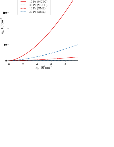
Figure 2: Particle number density as a function of the electron number density at $a=1\;\mu{\mbox{m}}$ for argon pressure of $10$ and $30\;{\mbox{Pa}}$ (MCEC, solid and dashed line, respectively). Dash-dot and dot line indicate the OML-based calculations Zhukhovitskii (2017) for $10$ and $30\;{\mbox{Pa}}$, respectively. $T_{e}=3.8{\kern 1.0pt}\,{\mbox{eV}}$.

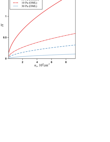
Figure 3: Havnes parameter as a function of the electron number density at $a=1\;\mu{\mbox{m}}$ for argon pressure of $10$ and $30\;{\mbox{Pa}}$ (MCEC, solid and dashed line, respectively). Dash-dot and dot line indicate the OML-based calculations Zhukhovitskii (2017) for $10$ and $30\;{\mbox{Pa}}$, respectively. $T_{e}=3.8{\kern 1.0pt}\,{\mbox{eV}}$.

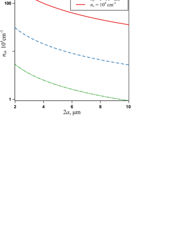
Figure 4: Particle number density as a function of the dust particle diameter at $p_{\mathrm{Ar}}=10\;{\mbox{Pa}}$ for the electron number density of $10^{8}{\kern 1.0pt}{\mbox{cm}}^{-3}$, $3\times 10^{8}{\kern 1.0pt}{\mbox{cm}}^{-3}$, and $10^{9}{\kern 1.0pt}{\mbox{cm}}^{-3}$ (dash-dot, dashed, and solid line, respectively). $T_{e}=3.8{\kern 1.0pt}\,{\mbox{eV}}$.

The increase of $n_{d}$ with the increase of $n_{e}$ stipulates the increase of the Havnes parameter (Fig. 3). This effect is especially noticeable at low argon pressure. Since the OML approximation leads to lower $n_{d}$ (cf. Fig. 2), resulting $H$ is lower as well, as compared to the present approach including the ion current enhancement. However, note that in the OML approximation, $n_{e}$ corresponding to the experimentally measured $n_{d}$ is one or two orders of magnitude higher than that shown in Fig. 3 (cf. Naumkin et al. (2016)). Eventually, in the present approximation, $H$ proves to be significantly lower than that from the OML. It can be seen in Fig. 3 that $H<1$ for $n_{e}$ characteristic of the available experimental data. This means that in many cases, one can neglect the perturbation of $n_{e}$ caused by the particles injection (this may not be true in the region adjacent to the void boundary because of the particle number density cusp Naumkin et al. (2016)). Thus for a quasi-homogeneous dust cloud (in the foot region Naumkin et al. (2016)), a reasonable estimate for complex plasma parameters can be based on the electron number density calculated for a discharge in a pure gas.

In the case $H\ll 1$, the particle dimensionless potential is not much different from its upper bound $\Phi_{0}$ corresponding to the limit $n_{d}\to 0$ or $n_{e}\to n_{i}$. From (9), we have $\Phi_{0}\simeq\theta^{-1/3}$. Using (10) we obtain $\Phi_{0}\simeq 0.23$ for $a=2\times 10^{-4}\,{\mbox{cm}}$ and $p_{\mathrm{Ar}}=30\;{\mbox{Pa}}$. In the entire range of experimentally attainable argon pressures and particle diameters, $0.2\lesssim\Phi_{0}\lesssim 0.3$, which is more than four times smaller than the particle potential calculated using the OML. This agrees with the results of recent particle charge measurements Saitou (2018). Figure 4 demonstrates the decreasing dependence of $n_{d}$ on the particle size at fixed $n_{e}$. This dependence is rather weak in contrast to a sharp dependence on $n_{e}$ illustrated again by this figure.

The developed IEOS’s (15), (18), and (19) are based on the assumption that the Coulomb potentials of neighboring particles overlap; Eq. (12) assumes explicitly that the ion–particle scattering is equivalent to the collisions of the ions against a hard sphere with the radius $0.45r_{d}$. Thus, the proposed model is valid if the latter does not exceed the length scale $a\tau\Phi$ defining the Coulomb cross section of the momentum transfer from an ion to the particle, i.e.,

$$\chi=\displaystyle{{2.2a\tau\Phi}\over{r_{d}}}\geq 1.$$ (21)

As is seen in Fig. 2, the particle number density decreases with the increase of the gas pressure other parameters being fixed, and $r_{d}$ increases. Therefore, the condition (21) imposes an upper bound on the gas pressure. If $n_{e}$ is decreased with the decreasing gas pressure then $r_{d}$ is increased, which implies a lower bound on the particle number density and the gas pressure. However, explicit estimates for these bounds cannot be deduced because the general form of the dependence $n_{e}(p_{\mathrm{Ar}})$ is yet unknown.

V COMPARISON WITH EXPERIMENTAL DATA

Comparison of the IEOS calculation results with experimental data is complicated by the fact that no measurement of the electron/ion number density is available and that the accurate particle number density determination using different methods was performed only in Khrapak et al. (2012); Naumkin et al. (2016). A qualitative conclusion that $n_{d}$ must decrease with the increase of $p_{\mathrm{Ar}}$ (Fig. 2) agrees with the experiment Naumkin et al. (2016), according to which the dust cloud can be realized in two regimes. At the lower $p_{\mathrm{Ar}}$, $n_{d}$ decreases monotonically with the distance from the discharge center; at the higher $p_{\mathrm{Ar}}$, $n_{d}$ is almost constant. Existence of these two regimes can be accounted for by the weaker dependence $n_{d}(n_{e})$ at the higher $p_{\mathrm{Ar}}$. In addition, the spatial distribution of $n_{e}$ in a gas discharge without particles can be more homogeneous at the higher $p_{\mathrm{Ar}}$. Thus, the IEOS modification proposed in this work is capable of describing the dependence of the particle number density on the gas pressure.

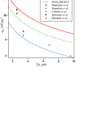
Figure 5: Particle number density as a function of the dust particle diameter for the electron number density $n_{e}=3.5\times 10^{8}{\kern 1.0pt}{\mbox{cm}}^{-3}$ and different argon pressures. Lines indicate calculations for $p_{\mathrm{Ar}}=10\;{\mbox{Pa}}$, $T_{e}=3.5\;{\mbox{eV}}$ (solid line), $15\;{\mbox{Pa}}{\mbox{,}}\;\;3.8\;{\mbox{eV}}$ (dashed line), and $30\;{\mbox{Pa}}{\mbox{,}}\;\;4.5\;{\mbox{eV}}$ (dash-dot line). Dots represent experiments Naumkin et al. (2016) (circles for $p_{\mathrm{Ar}}=10$ and squares, for $20.5\;{\mbox{Pa}}$), Caliebe et al. (2011) (triangle for $p_{\mathrm{Ar}}=30\;{\mbox{Pa}}$), Schwabe et al. (2011) (diamond for $p_{\mathrm{Ar}}=10\;{\mbox{Pa}}$), and Khrapak et al. (2012) (open triangles for $p_{\mathrm{Ar}}=15\;{\mbox{Pa}}$) (see Table 1).

Table 1: Estimations of the Havnes parameter $H$ Eq. (20), of the parameter $\chi=2.2a\tau\Phi/r_{d}$, and of the electron number density $n_{e}$ from Eqs. (15), (18), and (19) compared to that from the OML-based model Zhukhovitskii (2017) $n_{e}^{\mathrm{(OML)}}$, in a quasi-homogeneous region of the dust cloud in argon discharge based on the experimental data (the particle diameter $2a$, the argon pressure $p_{\mathrm{Ar}}$, the electron temperature $T_{e}$, and the particle number density $n_{d}$).

$2a,\;10^{-4}{\kern 1.0pt}{\mbox{cm}}$	$p_{\mathrm{Ar}},\;{\mbox{Pa}}$	$T_{e},\;{\mbox{eV}}$	$n_{d},\;10^{4}{\kern 1.0pt}{\kern 1.0pt}{\mbox{cm}}^{-3}$	Reference	$H$	$\chi$	$n_{e},\;10^{8}{\kern 1.0pt}{\kern 1.0pt}{\mbox{cm}}^{-3}$	$n_{e}^{\mathrm{(OML)}},\;10^{8}{\kern 1.0pt}{\kern 1.0pt}{\mbox{cm}}^{-3}$
1.55	15	3.8	65.2	[Khrapak et al., 2012]	0.723	1.08	5.60	35.2
2.55	15	3.8	26.7	[Khrapak et al., 2012]	0.537	1.17	4.52	33.2
9.55	30	4.5	1.97	[Caliebe et al., 2011]	0.113	1.13	3.64	56.0
2.55	10	3.5	22.3	[Schwabe et al., 2011]	0.760	1.17	2.89	17.5
2.55	10	3.5	28.0	[Naumkin et al., 2016]	0.818	1.25	3.27	20.1
3.4	11	3.5	8.01	[Naumkin et al., 2016]	0.491	1.04	1.98	13.7
3.4	20.5	3.5	6.30	[Naumkin et al., 2016]	0.243	0.84	2.73	23.1
6.8	20.5	3.5	3.65	[Naumkin et al., 2016]	0.202	1.14	3.10	32.4

A quantitative correspondence between the proposed IEOS and experiments performed with the particles of different diameters can be seen in Fig. 5. Since the electron number density at the point of $n_{d}$ measurement is unknown, we chose the common value of $n_{e}=3.5\times 10^{8}{\kern 1.0pt}{\mbox{cm}}^{-3}$ most typical for the discharge in a pure gas under the same discharge conditions. However, the dependence $n_{d}(n_{e})$ is rather sharp. One should also bear in mind that each experiment is performed under individual argon pressure (see Table 1), so we took three average pressures, $10$, $15$, and $30\;{\mbox{Pa}}$ to juxtapose with the experimental data, which are represented by the dots colored in the same way as the closest pressure in the calculations. In view of the foregoing, a satisfactory agreement between the proposed IEOS and the experimental data can be testified in a wide range of the particle diameter. A good reproduction of the trends under variation of both the gas pressure and the particle diameter can be seen in Fig. 5.

Note that only the experiments performed under microgravity conditions were selected for comparison with the obtained theoretical results in Fig. 5. Since the gravity adds a substantial additional force to those treated in the proposed model, this model cannot be used for the conditions of ground-based laboratory experiments. Thus, a correction in the theory is needed to implement it to such experiments.

Based on the data of experiments Khrapak et al. (2012); Caliebe et al. (2011); Schwabe et al. (2011); Naumkin et al. (2016) one can solve the inverse problem, i.e., calculate the electron number density at the point where $n_{d}$ was measured. The calculation results are summarized in Table 1 where the corresponding Havnes parameter is given along with $n_{e}$. It can be seen that in a wide range of the particle diameter and number density (more than one order of magnitude), the resulting $n_{e}$ varies in a restricted range from $2\times 10^{8}$ to $5\times 10^{8}{\kern 1.0pt}{\kern 1.0pt}{\mbox{cm}}^{-3}$. This is a consequence of the above-mentioned sharp dependence $n_{d}(n_{e})$. At the same time, estimated $n_{e}$ seems to be reasonable for treated discharge conditions. In contrast, the electron number densities obtained from the OML-based IEOS Zhukhovitskii (2017) are more than by an order of magnitude higher and they almost reach $10^{10}{\kern 1.0pt}{\kern 1.0pt}{\mbox{cm}}^{-3}$, which seams quite unrealistic for the treated experimental conditions. Calculation of the parameters makes it possible to check the condition of MCEC validity (21). It is seen that the condition is satisfied for almost all the experiments but one for $2a=3.4\;\mu{\mbox{m}}$ and $p_{\mathrm{Ar}}=20.5\;{\mbox{Pa}}$. However for all experiments, $\chi\simeq 1$. This makes the condition (21) compatible with $1.5a\tau\Phi/r_{d}=0.68\chi\lesssim 1$, which is necessary to reduce (7) to (8).

Note that although $H$ is noticeably higher for small particles, still $H<1$, which is indicative of a moderate (or small) effect of the particles on the electron number density in argon discharge plasma.

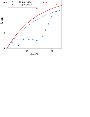
Figure 6: Difference $\delta=n_{d}^{-1/3}-n_{d}^{-1/3}\left|{{}_{p_{\mathrm{Ar}}=11{\kern 1.0pt}\mathrm{Pa}}}\right.$ as a function of the argon pressure for $2a=1.55\;\mu{\mbox{m}}$ (dashed line and circles) and $2.55\;\mu{\mbox{m}}$ (solid line and diamonds). Lines represent calculations and dots, the experimentKhrapak et al. (2012).

In the discussion above, we considered the dependence of $n_{d}$ on $p_{\mathrm{Ar}}$ at fixed $n_{e}$, i.e., solely the dependence $\lambda_{a}(p_{\mathrm{Ar}})$ is taken into account. Instead, in a real system, $n_{e}$ depends on $p_{\mathrm{Ar}}$ as well. In the center of pure argon discharge, this dependence was approximated by the linear functionKhrapak et al. (2012)

$$n_{e}=(1.20{\mbox{ }}+{\mbox{ }}0.11p_{\mathrm{Ar}})\times 10^{8}{\kern 1.0pt}{\kern 1.0pt}{\mbox{cm}}^{-3},$$ (22)

where $p_{\mathrm{Ar}}$ is in Pa. We will neglect the change of $n_{e}$ upon injection of the particles. Since $n_{d}$ decreases with the increase of $p_{\mathrm{Ar}}$ at fixed $n_{e}$ and increases with the increase of $n_{e}$ at fixed $p_{\mathrm{Ar}}$, the net dependence of $n_{d}$ on $p_{\mathrm{Ar}}$ is not clear if $n_{e}$ is related to $p_{\mathrm{Ar}}$. In so doing, one should bear in mind that the particle number density was measured in Khrapak et al. (2012) outside the discharge central region so that $n_{e}$ (22) does not coincide with a true electron number density at the measurement point. Hence, if we calculated $n_{d}$ with (22), the error could be too great. However, one can assume that the variation rate $dn_{e}/dp_{\mathrm{Ar}}$ is weakly dependent on the coordinate of measurement point. Then it is reasonable to calculate the difference $\delta$ between the interparticle distance $n_{d}^{-1/3}(p_{\mathrm{Ar}})$ and this quantity at some fixed pressure ($11\;{\mbox{Pa}}$). We used (22) to calculate such difference. Figure 6 shows the comparison of calculation results for two particle diameters with the measured dependences of the interparticle distance on the pressure. Note that the measurement of $n_{d}^{-1/3}(p_{\mathrm{Ar}})$ Khrapak et al. (2012) was dynamic rather than static so that the effect of the rate of $p_{\mathrm{Ar}}$ variation could be nonzero. Apparently, the latter is responsible for a kinky arrangement of the experimental dots. To avoid the mess, we reproduce a single branch of the hysteresis corresponding to the maximum $p_{\mathrm{Ar}}$ attained for each particle diameter. Obviously, dynamic effects cannot be included in the proposed IEOS. As is seen in Fig. 6, the decreasing dependence $n_{d}(p_{\mathrm{Ar}})$ dominates the increasing dependence $n_{d}(n_{e})$ so that the overall effect is the decrease of $n_{d}$ (increase of $n_{d}^{-1/3}$) with the increase of $p_{\mathrm{Ar}}$. This is in a qualitative agreement with the experiment. Another qualitative correspondence is the faster increase of $n_{d}^{-1/3}(p_{\mathrm{Ar}})$ with the increase of $p_{\mathrm{Ar}}$ for the larger particles. Note a satisfactory quantitative agreement between the calculated and measured $\delta$ at the highest pressure. Furthermore, it is worth mentioning that the calculation formulas (15), (18), and (19) used for Figs. 5 and 6 are free from fitting parameters. Therefore, they can be used for predictive calculations in planning the future experiments.

VI SPALLATION THRESHOLD FOR THE DUST CLOUD

Due to the strong Coulomb coupling, the dense cloud of dust particles contained in the electrostatic trap form an analog of condensed matter. Under certain conditions, spallation of such liquid or solid can occur. For example, we can consider spallation caused by the presence of a single probe particle of the radius $a_{p}\neq a$. It was demonstrated Zhukhovitskii (2017) that the sum of the ion drag force and the electrostatic force, ${\bf{F}}_{ip}$ and ${\bf{F}}_{ep}$, respectively, acting on the probe particle that we term the driving force ${\bf{F}}_{\mathrm{drv}}$ does not vanish (${\bf{F}}_{ip}$, ${\bf{F}}_{ep}$, and ${\bf{F}}_{\mathrm{drv}}$ are parallel to the electric field strength ${\bf{E}}$). This is a result of the dependence of the ion mean free path on the particle number density. The force ${\bf{F}}_{\mathrm{drv}}$ drives the probe to the discharge center if $a_{p}<a$ and in the opposite direction otherwise. For the following, we will define the direction of the coordinate axis $X$ apart from the void center as a positive direction (this axis is parallel to ${\bf{E}}$) and treat the projection of the forces on $X$. If $F_{\mathrm{drv}}$ is sufficiently weak, the probe would diffuse through the cloud. In the case of a dust crystal, the diffusion would occur due to the local plastic deformations of a crystal. If $F_{\mathrm{drv}}$ exceeds some threshold, the probe would displace the dust particles from its rectilinear path. Thus, the dust particle displacement from the cylinder of the radius $R_{p}$, where $R_{p}$ is the radius of the probe Wigner–Seitz cell, should be considered. Then at the spallation threshold, the work of the driving force along the unit probe path $\left|{F_{\mathrm{drv}}}\right|$ is equal to the work $\pi pR_{p}^{2}$ against the pressure $p$ of the dust particles subsystem. Since the interparticle interaction is purely repulsive, $p$ is always positive. The moving probe can thus make a space free from the dust particles or a lane. Apparently, this effect is similar to the spallation of condensed matter (e.g., upon application of a negative pressure). The minimum driving force, at which this effect can emerge, is defined by the threshold condition $Q=1$, where

$$Q=\displaystyle{{\left|{F_{\mathrm{drv}}}\right|}\over{\pi pR_{p}^{2}}}.$$ (23)

One can estimate the spallation criterion $Q$ by calculation of $F_{\mathrm{drv}}$ in the same way as in Zhukhovitskii (2017). By definition, ${\bf{F}}_{\mathrm{drv}}={\bf{F}}_{ep}+{\bf{F}}_{ip}$. Here, $F_{ep}=-a_{p}T_{e}\Phi_{p}E/e$, where $\Phi_{p}$ is the probe potential defined by the probe charge equation. The latter has the form [cf. (9) and (10)]

$$\theta\Phi_{p}^{3}\displaystyle{{a_{p}}\over a}\exp\left({\Phi_{p}}\right)=1-\gamma(\Phi).$$ (24)

The ion drag force is then $F_{ip}=(\pi/2)R_{p}^{2}n_{i}\lambda_{p}eE$, where $R_{p}$ is defined by the relation Zhukhovitskii et al. (2014)

$$R_{p}^{2}=\displaystyle{{Z_{p}e^{2}}\over{(8\pi p)^{1/2}}}=\left({\displaystyle{{\rho\lambda_{a}}\over S}}\right)^{2},$$ (25)

and $S=\left({a\Phi/a_{p}\Phi_{p}}\right)^{1/2}$. Here, we took into account that $\Phi_{p}=Z_{p}e^{2}/a_{p}T_{e}$. In contrast to Eq. (18) in Zhukhovitskii (2017), Eq. (25) includes the ratio $\Phi_{p}/\Phi$. The local ion mean free path in the vicinity of a probe is defined by the approximation similar to (11) (cf. Zhukhovitskii (2017))

$$\lambda_{p}=\lambda_{a}\left({1+\displaystyle{{3\lambda_{a}}\over{8R_{p}}}}\right)^{-1}=\lambda_{a}\left({1+\displaystyle{{3S}\over{8\rho}}}\right)^{-1}.$$ (26)

Thus, we obtain

$$\kappa\equiv\displaystyle{{F_{\mathrm{drv}}}\over{F_{ep}}}=\displaystyle{{S-1}\over{S+8\rho/3}},$$ (27)

and the driving force is

$$F_{\mathrm{drv}}=\displaystyle{{\kappa a_{p}\Phi_{p}T_{e}^{2}}\over{Le^{2}}},$$ (28)

where $L=\left|{\bm{\nabla}\ln n_{e}}\right|^{-1}$ is the length scale of the electron number density variation. Based on (23), (27), (28), and the estimation for the particle pressure Zhukhovitskii et al. (2014) $p=Z^{2}e^{2}/8\pi r_{d}^{4}$ we derive eventually the spallation criterion

$$Q=\displaystyle{{8\left|\kappa\right|r_{d}^{2}}\over{a\Phi L}},$$ (29)

which can be calculated for a stationary dust cloud on the basis of the IEOS’s (15), (18), and (19).

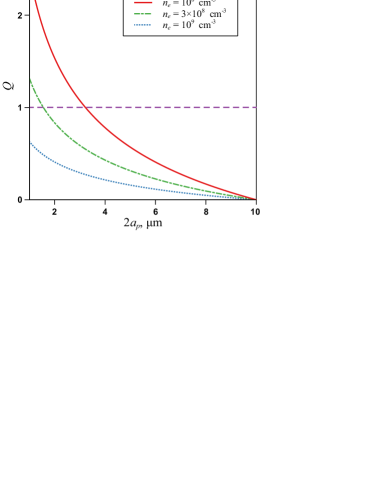
Figure 7: Spallation criterion (29) as a function of the probe particle diameter for the electron number density of $10^{8}{\kern 1.0pt}{\mbox{cm}}^{-3}$, $3\times 10^{8}{\kern 1.0pt}{\mbox{cm}}^{-3}$, and $10^{9}{\kern 1.0pt}{\mbox{cm}}^{-3}$ (sold, dash-dot, and dot line, respectively), $2a=10\;\mu{\mbox{m}}$, and $p_{\mathrm{Ar}}=30\;{\mbox{Pa}}$. Dashed line indicates the spallation threshold. $L=5\;{\mbox{cm}}$ and $T_{e}=3.8{\kern 1.0pt}\,{\mbox{eV}}$.

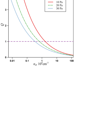
Figure 8: Spallation criterion (29) as a function of the dust particle number density for $p_{\mathrm{Ar}}=10$, $20$, and $30\;{\mbox{Pa}}$ (sold, dash-dot, and dot line, respectively), $2a=10\;\mu{\mbox{m}}$, and $2a_{p}=3\;\mu{\mbox{m}}$. Dashed line indicates the spallation threshold. $L=5\;{\mbox{cm}}$ and $T_{e}=3.8{\kern 1.0pt}\,{\mbox{eV}}$.

If the probe radius is close to that of the dust particles, $\left|{a-a_{p}}\right|/a\ll 1$ then one can use (27) to write approximately

$$\kappa\simeq\displaystyle{{\lambda_{a}}\over{8r_{d}+3\lambda_{a}}}\left({1-\displaystyle{{a_{p}}\over a}}\right).$$ (30)

From (29) and (30) for $\left|{a-a_{p}}\right|/a\sim 1$ and $\rho>3/8$, one can obtain a crude estimate $Q\simeq r_{d}\lambda_{a}/a\Phi L$. This means that spallation would be impossible for a dense system (small $r_{d}$) of large particles at high argon pressure. Since $Q\propto L^{-1}\propto E$, the ambipolar electric field must be sufficiently strong. In addition, the increase of $p_{\mathrm{Ar}}$ increases $r_{d}$ but decreases $\lambda_{a}$ and $\Phi$. As a result, $Q$ is almost independent of the argon pressure at fixed $n_{e}$.

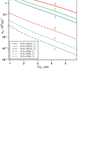
Figure 9: Particle number density along the line $Q=1$ (spallation threshold) as a function of the probe particle diameter for $2a=9.2\;\mu{\mbox{m}}$ and the argon pressure of (1) $10$, (2) $20$, and (3) $30\;{\mbox{Pa}}$ (MCEC). Dashed lines indicate similar results from the OML-based IEOS Zhukhovitskii (2017) for the argon pressure of (1) $10$, (2) $20$, and (3) $30\;{\mbox{Pa}}$. $L=5\;{\mbox{cm}}$ and $T_{e}=3.8{\kern 1.0pt}\,{\mbox{eV}}$.

The objective of the following calculations is to clarify the conditions, under which spallation is favored. In so doing, we will confine ourselves to the case $a>a_{p}$ and assume a quasi-homogeneous dust cloud in the argon discharge. Then the estimation of the length scale $L\sim 5\;{\mbox{cm}}$ in (29) can be of the same order as typical discharge dimensions. Figure 7 illustrates the spallation accessibility for different probe diameters provided that the dust particle diameter and the argon pressure are fixed. As is seen, spallation is impossible as $a_{p}\to a$; this follows straightforwardly from (29) and (30). Spallation is hindered for high electron number density as well because of the associated increase of $n_{d}$. It follows from Fig. 7 that spallation is possible for a probe of the diameter about $4\;\mu{\mbox{m}}$ at the typical level of $n_{e}\sim 10^{8}\,{\mbox{cm}}^{-3}$. Figure 8 shows that the increase of the argon pressure other parameters being fixed increases $Q$. The particle number density, at which spallation is possible, ranges between $10^{3}$ and $10^{4}\,{\mbox{cm}}^{-3}$.

The set of Eqs.  (15), (18), and (19) combined with the threshold condition $Q=1$ define uniquely the parameters of complex plasma such as the threshold particle number density for given probe diameter (Fig. 9). This figure demonstrates that the decrease in argon pressure favors spallation, i.e., it shifts the threshold line toward the region of the denser and more strongly coupled system. It is seen that for $2a_{p}=3.4\;\mu{\mbox{m}}$, $2a=9.2\;\mu{\mbox{m}}$, and $p_{\mathrm{Ar}}=30\;{\mbox{Pa}}$, the threshold particle number density $10^{3}\lesssim n_{d}\lesssim 10^{4}\,{\mbox{cm}}^{-3}$. This agrees with the result of experiment Sütterlin et al. (2009), in which a beam of smaller particles penetrated a quasi-homogeneous stationary cloud of the larger dust particles thus forming lanes. The particle diameters and argon pressure are specified above. Judging from Fig. 1 of Sütterlin et al. (2009), the experimental particle number density can be in the same range from ca. $10^{3}$ to $10^{4}\,{\mbox{cm}}^{-3}$. For comparison, Fig. 9 also shows the line $Q=1$, where the quantities included in (29) are calculated using the OML-based IEOS Zhukhovitskii (2017). It is seen that the threshold particle number densities are up to three orders of magnitude lower than those calculated in this work. Thus, consideration of the ion–atom collisions is fundamentally important for the treatment of lane formation.

Note that the spallation criterion for a beam of particles can be different from that for a single probe particle. In addition, it is a matter of discussion whether the lane formation observed in Sütterlin et al. (2009) can be treated as the spallation.

VII CONCLUSION

In this study, we propose a modification of the IEOS that includes the effect of the ion–atom collisions in the vicinity of dust particles. Toward this end, we estimated the screening length for the “dense” dust cloud in the framework of the Wigner–Seitz cell model. This screening length proved to be typically larger than the ion Debye screening length. Fortunately, it cancels in the expression for ion current to the particle (8) and, correspondingly, in the equations for the particle charge (9), (10). Inclusion of the ion–atom collisions leads to more than an order of magnitude increase in the estimated ion current (this effect is proportional to $a/\lambda_{a}$), which implies the decrease of the particle charge $Z$. It was demonstrated that the necessary condition to treat collisionless plasma is $\lambda_{a}/r_{d}>10$, which demonstrates the importance of included effect.

The IEOS’s for a dense dust cloud in the low-pressure gas discharge are based on the particle charge equation, the quasineutrality equation, and the balance equation for the electrostatic force and the ion drag force acting on a particle. The latter force takes into account both the effects of the ion–atom and that of the ion–particle collisions. It follows from obtained IEOS’s that the particle number density decreases with the increase of the particle diameter and the gas pressure and it increases rather sharply with the increase of the electron number density. Since in a real discharge, the latter is, in its turn, dependent on the gas pressure, the performed calculations took into account this dependence. Comparison between the theory and available experimental data concerning the particle number densities is indicative of a satisfactory quantitative agreement in a wide range of variation of complex plasma parameters. In particular, calculations demonstrate the net effect of the decrease of $n_{d}$ with the increase of $p_{\mathrm{Ar}}$. Note that used IEOS’s includes no fitting parameters.

The following shortcomings of the proposed theory should be noted. The inapplicability of this theory for the interpretation of ground-based experiments has already been noted in Sec. V. Next, the implementation of IEOS’s implies that one of the complex plasma parameters is known. Calculation of all plasma parameters would require incorporation of IEOS’s with the equations for the ionization kinetics. Then, the proposed theory is local, which implies that all quantities are at least continuous. This is not true in the vicinity of the void boundary (in the cusp region Naumkin et al. (2016)), where $n_{d}$ changes abruptly. In this region, the theory is invalid.

Obtained IEOS’s proved to have sufficient accuracy to estimate the threshold of the lane formation, which is sensitive to the plasma parameters. We assume that emergence of the lanes upon injection of small dust particles (probes) into a cloud of large particles is a manifestation of spallation of the plasma crystal caused by the probes. In contrast to the lane formation in colloidal mixtures, this could rather be similar to spinodal decay than to a nonequilibrium phase transition. The probe particle in a dust cloud that is of the size different from that of the cloud particles is subject to the driving force, which is a result of the dependence of the local ion mean free path and, correspondingly, of the ion driving force on the particle size. The moving probe particle can form a cylindrical cavity if the work of driving force is greater than the work against the positive pressure of the cloud particles. This enables one to obtain the spallation criterion that can be calculated on the basis of IEOS’s. The calculations show that the lane formation is possible provided that the size difference between the probe and the cloud particles is sufficiently large, and if the electron and particle number density is sufficiently low. The lane formation onset criterion increases, i.e., the threshold decreases, with the decreasing gas pressure. We demonstrate that under the conditions of experiment Sütterlin et al. (2009), the threshold number density of the cloud particles must be in the interval $10^{3}\lesssim n_{d}\lesssim 10^{4}\,{\mbox{cm}}^{-3}$, which agrees with experimental data. Apparently, this interval can be typical for similar experiments. Since no experimental information on the lane formation threshold is available, conducting new experiments, in which this threshold can be measured and its dependence on plasma parameters can be determined, is an urgent task in this field. The theory proposed in this work treats solely individual probes and does not take into account the collective motion of such particles. The open issues mentioned above will be addressed in the future.