Strong decays of double-charmed pseudoscalar and scalar $cc\overline{u}\overline{d}$ tetraquarks

Abstract

The strong decays of the pseudoscalar and scalar double-charmed tetraquarks $T_{cc;\overline{u}\overline{d}}^{+}$ and $\widetilde{T}_{cc;\overline{u}\overline{d}}^{+}$ are investigated in the framework of the QCD sum rule method. The mass and coupling of these exotic four-quark mesons are calculated in the framework of the QCD two-point sum rule approach by taking into account vacuum condensates of the quark, gluon, and mixed local operators up to dimension 10. Our results for masses $m_{T}=(4130~{}\pm 170)~{}\mathrm{MeV}$ and $m_{\widetilde{T}}=(3845~{}\pm 175)~{}\mathrm{MeV}$ demonstrate that these tetraquarks are strong-interaction unstable resonances and decay to conventional mesons through the channels $T_{cc;\overline{u}\overline{d}}^{+}\to D^{+}D^{\ast}(2007)^{0},~{}D^{0}D^{\ast}(2010)^{+}$ and $\widetilde{T}_{cc;\overline{u}\overline{d}}^{+}\to D^{+}D^{0}$. Key quantities necessary to compute the partial width of these decay modes, i.e., the strong couplings of two $D$ mesons and a corresponding tetraquark $g_{i},~{}i=1,2$, and $G$ are extracted from the QCD three-point sum rules. The full width $\Gamma_{T}=(129.9\pm 23.5)~{}\mathrm{MeV}$ demonstrates that the tetraquark $T_{cc;\overline{u}\overline{d}}^{+}$ is a broad resonance, whereas the scalar exotic meson with $\Gamma_{\widetilde{T}}=(12.4\pm 3.1)~{}\mathrm{MeV}$ can be classified as a relatively narrow state.

I Introduction

Double-charmed tetraquarks as exotic mesons are already on agenda of high-energy physics. Their properties were studied in a more general context of double-heavy mesons built of a heavy diquark $QQ$ and heavy or light antidiquarks Ader:1981db ; Lipkin:1986dw ; Zouzou:1986qh ; Carlson:1987hh . A main question addressed in these basic papers was whether such 4-quarks can form bound states or exist as unstable resonances. It was demonstrated that exotic mesons $QQ\overline{q}\overline{q}$ might be stable provided that the mass ratio of constituent quarks $m_{Q}/m_{q}$ is large enough. In this sense, tetraquarks with a diquark $bb$ are more promising candidates to stable exotic mesons than ones containing a $bc$ or $cc$ pair. In fact, the isoscalar $J^{P}=1^{+}$ tetraquark $T_{bb;\bar{u}\bar{d}}^{-}$ is expected to lie below the two $B$-meson threshold and is strong-interaction stable state Carlson:1987hh . The situation with $T_{bc;\bar{q}\bar{q}^{\prime}}$ and $T_{cc;\bar{q}\bar{q}^{\prime}}$ is not quite clear; they may exist as either bound or resonant states.

In the following years the chiral quark model, dynamical and relativistic quark models, and other theoretical schemes of high-energy physics were used to calculate spectroscopic parameters of the double-charmed tetraquarks Pepin:1996id ; Cui:2006mp ; Vijande:2006jf ; Ebert:2007rn . Production of these particles in ion, proton-proton, and electron-positron collisions, in $B_{c}$ and $\Xi_{bc}$ decays was investigated as well SchaffnerBielich:1998ci ; DelFabbro:2004ta ; Lee:2007tn ; Hyodo:2012pm ; Esposito:2013fma . In the framework of the QCD sum rule method the axial-vector tetraquarks $QQ\bar{u}\bar{d}$ were explored in Ref. Navarra:2007yw . In accordance with obtained results the mass of $T_{bb;\bar{u}\bar{d}}^{-}$ is below the open bottom threshold and, hence, it cannot decay directly to conventional mesons. Within the same method tetraquarks with quantum numbers $J^{P}=0^{-},~{}0^{+},~{}1^{-}$ and $1^{+}$, and the quark content $QQ\bar{q}\bar{q}$ were studied in Ref. Du:2012wp .

Recent intensive investigations of double-heavy tetraquarks were inspired by the discovery of double-charmed baryon $\Xi_{cc}^{++}=ccu$ Aaij:2017ueg . The mass of this particle was utilized as input information in a phenomenological model to evaluate masses of the tetraquarks $T_{bb;\overline{u}\overline{d}}^{-}$ and $T_{cc;\overline{u}\overline{d}}^{+}$ Karliner:2017qjm . It was confirmed once more that the axial-vector isoscalar state $T_{bb;\overline{u}\overline{d}}^{-}$ is stable against strong and electromagnetic interactions, whereas the tetraquark $T_{cc;\overline{u}\overline{d}}^{+}$ can decay to $D^{0}D^{\ast+}$ mesons. A conclusion on a stable nature of $T_{bb;\overline{u}\overline{d}}^{-}$ was drawn also in Refs. Eichten:2017ffp ; Agaev:2018khe .

The spectroscopic parameters and widths of the double-charmed pseudoscalar tetraquarks $T_{cc;\overline{s}\overline{s}}^{++}$ and $T_{cc;\overline{d}\overline{s}}^{++}$, which bear two units of the electric charge were calculated in Ref. Agaev:2018vag . Obtained results showed that these exotic mesons are rather broad resonances. Various aspects of double-charmed tetraquarks were analyzed also in the publications Wang:2017dtg ; Hyodo:2017hue ; Yan:2018gik ; Luo:2017eub ; Ali:2018ifm .

In the present work we investigate the pseudoscalar and scalar tetraquarks $T_{cc;\overline{u}\overline{d}}^{+}$ and $\widetilde{T}_{cc;\overline{u}\overline{d}}^{+}$. First, we calculate their spectroscopic parameters in the context of the QCD two-point sum rule method by taking into account nonperturbative contributions up to dimension ten. Our studies demonstrate that these exotic mesons are unstable resonances, and decay strongly to conventional mesons. The kinematically allowed decay modes $T_{cc;\overline{u}\overline{d}}^{+}\rightarrow D^{+}D^{\ast}(2007)^{+}$, $T_{cc;\overline{u}\overline{d}}^{+}\rightarrow D^{0}D^{\ast}(2010)^{+}$, and $\widetilde{T}_{cc;\overline{u}\overline{d}}^{+}\rightarrow D^{0}D^{+}$ are analyzed and their partial widths are found. To this end, we consider the strong couplings of two $D$ mesons and tetraquarks, which are key quantities of the analysis, and extract their values from the three-point QCD sum rules. Obtained predictions are used to estimate the full width of the four-quark mesons $T_{cc;\overline{u}\overline{d}}^{+}$ and $\widetilde{T}_{cc;\overline{u}\overline{d}}^{+}$.

This work has the following structure. In Sec. II, we calculate the mass and coupling of the tetraquarks $T_{cc;\overline{u}\overline{d}}^{+}$ and $\widetilde{T}_{cc;\overline{u}\overline{d}}^{+}$. Here, we provide details of calculations for the pseudoscalar state $T_{cc;\overline{u}\overline{d}}^{+}$ and write down final predictions for $\widetilde{T}_{cc;\overline{u}\overline{d}}^{+}$. Section III is devoted to analysis of strong decays of the tetraquarks. For these purposes, we evaluate the couplings $g_{1}(q^{2})$, $g_{2}(q^{2})$ and $G(q^{2})$ corresponding to relevant strong vertices, and find the fit functions to extrapolate sum rule predictions to the relevant $D$ mesons’ mass shell.  These strong couplings are utilized to evaluate partial width of decay processes. Our conclusions are presented in Sec. IV.

II Mass and coupling of the pseudoscalar and scalar tetraquarks $T_{cc;\overline{u}\overline{d}}^{+}$ and $\widetilde{T}_{cc;\overline{u}\overline{d}}^{+}$

As it has been noted above, the mass and coupling of the tetraquarks $T_{cc;\overline{u}\overline{d}}^{+}$ and $\widetilde{T}_{cc;\overline{u}\overline{d}}^{+}$ (in what follows denoted by $T$ and $\widetilde{T}$, respectively) can be evaluated by means of the QCD two-point sum rule method. The essential component of this approach is the interpolating current, which should be composed of relevant diquark fields and has the quantum numbers of the original particle. There are different currents that meet these requirements Du:2012wp . For the pseudoscalar tetraquark $T$ with two identical $c$ quarks we choose a structure made of the heavy pseudoscalar and light scalar diquarks

$$J(x)=c_{a}^{T}(x)Cc_{b}(x)\overline{u}_{a}(x)\gamma_{5}C\overline{d}_{b}^{T}(x).$$ (1)

The current $J(x)$ has the symmetric color structure and belongs to the sextet representation of the color group. The state $T$ with structure (1) is a $\overline{u}\overline{d}$ member of the multiplet of pseudoscalar $cc$ tetraquarks while others are the four-quark mesons $T_{cc;\overline{s}\overline{s}}^{++}$ and $T_{cc;\overline{d}\overline{s}}^{++}$. The present investigation allows us to add the new particle $T$ to the list of double-charmed pseudoscalar tetraquarks.

The interpolating current for the scalar tetraquark $\widetilde{T}$ can be constructed from the heavy and light axial-vector diquark fields Wang:2017dtg

$$\widetilde{J}(x)=\epsilon\widetilde{\epsilon}[c_{b}^{T}(x)C\gamma_{\mu}c_{c}(x)][\overline{u}_{d}(x)\gamma^{\mu}C\overline{d}_{e}^{T}(x)],$$ (2)

where $\epsilon\widetilde{\epsilon}=\epsilon^{abc}\epsilon^{ade}$. In expressions above, $a,b,c,d$, and $e$ are color indices, and $C$ is the charge-conjugation operator.

The QCD two-point sum rules to evaluate the spectroscopic parameters of the tetraquark $T$ should be derived from the correlation function

$$\Pi(p)=i\int d^{4}xe^{ip\cdot x}\langle 0|\mathcal{T}\{J(x)J^{{\dagger}}(0)\}|0\rangle.$$ (3)

After replacement $J(x)\rightarrow\widetilde{J}(x)$ a similar correlator can be written down for the second particle $\widetilde{T}$ as well. Below we give details of calculations for the mass $m_{T}$ and coupling $f_{T}$, and provide only final results for $\widetilde{T}$.

To extract the desired sum rules from the correlation function $\Pi(p)$, one has, first of all, to express it in terms of the tetraquarks’ physical parameters and, in this way determine their phenomenological side $\Pi^{\mathrm{Phys}}(p)$. The function $\Pi^{\mathrm{Phys}}(p)$ can be derived by inserting into the correlation function $\Pi(p)$ a full set of relevant states, carrying out integration over $x$ in Eq. (3), and isolating a contribution of the ground-state particle $T$. In this process we accept an assumption on the dominance of a tetraquark term in the phenomenological side, which for multiquark hadrons should be applied with some caution. The reason is that an interpolating current used in such calculations couples not only to a multiquark hadron, but also to a relevant two-hadron continuum, which may obstruct the multiquark signal Kondo:2004cr . But direct subtraction of the two-hadron contributions from the correlator leads to wrong results and conclusions Lee:2004xk . To solve this problem, the authors in Ref. Lee:2004xk utilized an alternative way and computed explicitly a coupling of a two-hadron continuum with a pentaquark current, and demonstrated that these effects constitute less than $10\%$ of the sum rules.

A more general method to treat similar contributions in the sum rules involving tetraquarks was used in Ref. Wang:2015nwa . It turns out that two-meson continuum contributions give rise to the finite width $\Gamma(p^{2})$ of the tetraquark, which can be taken into account by modifying its propagator. In the sum rules, this modification leads to rescaling of the tetraquark’s coupling, while the mass remains unchanged. Our calculations showed that even for the tetraquarks with the full width of a few hundred mega-electron-volts, the two-meson continuum changed the coupling approximately by $(5-7)\%$ Agaev:2018vag ; Sundu:2018nxt . This uncertainty does not exceed the accuracy of the sum rule calculations themselves; therefore to derive $\Pi^{\mathrm{Phys}}(p)$ one can neglect it and use the zero-width single-pole approximation.

Then for $\Pi^{\mathrm{Phys}}(p)$ we get

$$\Pi^{\mathrm{Phys}}(p)=\frac{\langle 0|J|T(p)\rangle\langle T(p)|J^{\dagger}|0\rangle}{m_{T}^{2}-p^{2}}+\ldots,$$ (4)

which contains the contribution of the ground-state particle written down explicitly as well as effects due to higher resonances and continuum states: the latter in Eq. (4) is denoted by dots.

The correlation function $\Pi^{\mathrm{Phys}}(p)$ can be recast into a more simple form if one introduces the matrix element of the pseudoscalar tetraquark

$$\langle 0|J|T(p)\rangle=\frac{f_{T}m_{T}^{2}}{2m_{c}}.$$ (5)

Then, we find

$$\Pi^{\mathrm{Phys}}(p)=\frac{1}{4m_{c}^{2}}\frac{f_{T}^{2}m_{T}^{4}}{m_{T}^{2}-p^{2}}+\ldots$$ (6)

In general, to continue calculations one should choose in $\Pi^{\mathrm{Phys}}(p)$ some Lorentz structure and fix the corresponding invariant amplitude. Because in the case under discussion $\Pi^{\mathrm{Phys}}(p)$ has the trivial structure which is proportional to $I$, the amplitude $\Pi^{\mathrm{Phys}}(p^{2})$ equals the function from Eq. (6).

The QCD side of the sum rules $\Pi^{\mathrm{OPE}}(p)$ can be found by computing the correlation function in terms of the quark propagators. To this end, we insert the interpolating current $J(x)$ to the expression (3) and after contracting the relevant quark fields find

$$\Pi^{\mathrm{OPE}}(p)=i\int d^{4}xe^{ipx}\mathrm{Tr}\left[\gamma_{5}\widetilde{S}_{d}^{b^{\prime}b}(-x)\gamma_{5}S_{u}^{a^{\prime}a}(-x)\right]$$

$$\times\mathrm{Tr}\left[S_{c}^{bb^{\prime}}(x)\widetilde{S}_{c}^{aa^{\prime}}(x)+S_{c}^{ab^{\prime}}(x)\widetilde{S}_{c}^{ba^{\prime}}(x)\right].$$ (7)

Here, $S_{c}(x)$ and $S_{u(d)}(x)$ are the heavy $c$- and light $u(d)$-quark propagators, explicit expressions of which can be found, for example, in Ref. Sundu:2018uyi . In Eq. (7), we also introduce the shorthand notation

$$\widetilde{S}(x)=CS^{T}(x)C.$$ (8)

By equating the amplitudes $\Pi^{\mathrm{Phys}}(p^{2})$ and $\Pi^{\mathrm{OPE}}(p^{2})$, applying the Borel transformation to both sides of this expression, and performing the continuum subtraction, we get an equality, which can be used to derive sum rules for the mass $m_{T}$ and coupling $f_{T}$. The Borel transformation suppresses the contribution of higher resonances and continuum states and generates a dependence of the sum rules on a new parameter $M^{2}$. The continuum subtraction allows one, by invoking the assumption on the quark-hadron duality, to replace an unknown physical spectral density $\rho^{\mathrm{Phys}}(s)$ by $\rho^{\mathrm{OPE}}(s)$, which is calculable as an imaginary part of $\Pi^{\mathrm{OPE}}(p)$. A price paid for this simplification is appearance in the sum rules the continuum threshold parameter $s_{0}$ that separates from one another the ground-state and continuum contributions to $\Pi^{\mathrm{OPE}}(p^{2})$.

To derive the final sum rules, we use this equality as well as one obtained from the first expression by applying the operator $d/d(-1/M^{2})$. As a result, we get

$$m_{T}^{2}=\frac{\int_{4m_{c}^{2}}^{s_{0}}dss\rho^{\mathrm{OPE}}(s)e^{-s/M^{2}}}{\int_{4m_{c}^{2}}^{s_{0}}ds\rho^{\mathrm{OPE}}(s)e^{-s/M^{2}}},$$ (9)

and

$$f_{T}^{2}=\frac{4m_{c}^{2}}{m_{T}^{4}}\int_{4m_{c}^{2}}^{s_{0}}ds\rho^{\mathrm{OPE}}(s)e^{(m_{T}^{2}-s)/M^{2}}.$$ (10)

As we have noted above, Eqs. (9) and (10) depend the auxiliary parameters $M^{2}$ and $s_{0}$. Their values are related to a problem under analysis and should be fixed to satisfy constraints, which we explain below. But the sum rules contain also various vacuum condensates that are universal for all problems:

$$\langle\bar{q}q\rangle=-(0.24\pm 0.01)^{3}\ \mathrm{GeV}^{3},\$$

$$m_{0}^{2}=(0.8\pm 0.1)\ \mathrm{GeV}^{2},\ \langle\overline{q}g_{s}\sigma Gq\rangle=m_{0}^{2}\langle\overline{q}q\rangle,$$

$$\langle\frac{\alpha_{s}G^{2}}{\pi}\rangle=(0.012\pm 0.004)\,\mathrm{GeV}^{4},$$

$$\langle g_{s}^{3}G^{3}\rangle=(0.57\pm 0.29)~{}\mathrm{GeV}^{6}.$$ (11)

In numerical computations we use this information on vacuum condensates and the $c$-quark mass $m_{c}=1.275_{-0.035}^{+0.025}\ \mathrm{GeV}$. Our studies prove that the working regions for the parameters

$$M^{2}\in[4,\ 6]~{}\mathrm{GeV}^{2},\ s_{0}\in[20,\ 22]~{}\mathrm{GeV}^{2}$$ (12)

meet all restrictions imposed on $M^{2}$ and $s_{0}$.

The regions (12) are extracted from analysis of a pole contribution to the correlator and convergence of the sum rules. The pole contribution (PC)

$$\mathrm{PC}=\frac{\Pi(M^{2},s_{0})}{\Pi(M^{2},\infty)},$$ (13)

where $\Pi(M^{2},s_{0})$ is the Borel-transformed and subtracted invariant amplitude $\Pi^{\mathrm{OPE}}(p^{2})$, is one of the important quantities necessary to extract limits of the Borel parameter $(M_{\mathrm{min}}^{2},M_{\mathrm{max}}^{2})$. In accordance with our computations at $M_{\mathrm{min}}^{2}=4~{}\mathrm{GeV}^{2}$, the pole contribution amounts to $0.7$, whereas at $M_{\mathrm{max}}^{2}=6~{}\mathrm{GeV}^{2}$ it is $0.37$. But at the same time, a lower limit of the Borel parameter depends on the convergence of the operator product expansion (OPE). Restrictions imposed on $M^{2}$ by convergence of OPE can be analyzed by means of the ratio

$$R(M_{\mathrm{min}}^{2})=\frac{\Pi^{\mathrm{DimN}}(M_{\mathrm{min}}^{2},s_{0})}{\Pi(M_{\mathrm{min}}^{2},s_{0})}.$$ (14)

Here $\Pi^{\mathrm{DimN}}(M^{2},\ s_{0})$ is a contribution to the correlation function arising from the last term (or from the sum of last few terms) in OPE. Numerical analysis proves that for $\mathrm{DimN}=\mathrm{Dim(8+9+10)}$ this ratio is $R(4~{}\mathrm{GeV}^{2})=0.02$, which guarantees the convergence of the sum rules. It is worth noting that the lower boundary of the Borel window is determined from joint analysis of PC and $R(M_{\mathrm{min}}^{2})$, i.e., the maximum accessible pole contribution is limited by the convergence of the OPE. Additionally, at the minimum of the Borel parameter the perturbative term amounts to $68\%$ of the total result and exceeds the nonperturbative contributions.

In general, quantities extracted from the sum rules should not depend on the auxiliary parameters $M^{2}$ and $s_{0}$. In real calculations, however, we observe a residual dependence of $m_{T}$ and $f_{T}$ on them. Hence, the choice of $M^{2}$ and $s_{0}$ should minimize these nonphysical effects as well. The working windows for the parameters $M^{2}$ and $s_{0}$ also satisfy these conditions. In Figs. 1 and 2 we plot the mass $m_{T}$ and coupling $f_{T}$ as functions of $M^{2}$ and $s_{0}$, which allows one to see uncertainties generated by the sum rule computations. It is seen that both $m_{T}$ and $f_{T}$ depend on $M^{2}$ and $s_{0}$, which are main sources of the theoretical uncertainties inherent in the sum rule computations. For the mass $m_{T}$, these uncertainties are small, $\pm 4\%$, because the ratio in Eq. (9) cancels some of these effects. But even for the coupling $f_{T}$, the ambiguities do not exceed $\pm 20\%$ of the central value.

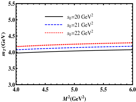
Figure 1: The mass of the tetraquark $T$ as a function of the Borel parameter $M^{2}$ (left panel) and as a function of the continuum threshold $s_{0}$ (right panel).

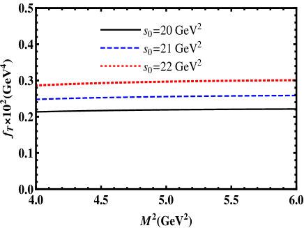
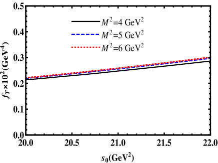
Figure 2: The same as in Fig. 1, but for the coupling $f_{T}$ of the state $T$.

Our calculations lead to the following results:

$$m_{T} = (4130~{}\pm 170)~{}\mathrm{MeV},$$

$$f_{T} = (0.26\pm 0.05)\times 10^{-2}\ \mathrm{GeV}^{4}.$$ (15)

The prediction for $m_{T}$ confirms that $T$ can be interpreted as a member of the multiplet formed by the double-charmed pseudoscalar tetraquarks. In fact, parameters of other members of this multiplet $T_{cc;\overline{s}\overline{s}}^{++}$ and $T_{cc;\overline{d}\overline{s}}^{++}$ were calculated in Ref. Agaev:2018vag . The mass splitting between these two states $125~{}\mathrm{MeV}$ is caused by the replacement $\overline{s}\leftrightarrow\overline{d}$ in their quark contents. By similar substitution $\overline{s}\rightarrow\overline{u}$ in $T_{cc;\overline{d}\overline{s}}^{++}$, one can create the tetraquark $T$ . Comparing now the mass $4265~{}\mathrm{MeV}$ of $T_{cc;\overline{d}\overline{s}}^{++}$ with $m_{T}=4130~{}~{}\mathrm{MeV}$, we find the mass difference $135~{}\mathrm{MeV}$ between these two particles. In other words, the state $T$ occupies an appropriate place in the multiplet of the double-charmed pseudoscalar tetraquarks, which we consider an important consistency check of the present result.

Let us also note that $m_{T}$ is considerably lower than $(4430\pm 130)~{}\mathrm{MeV}$ predicted in Ref. Du:2012wp for the pseudoscalar tetraquark with the same quark content and structure. This discrepancy presumably stems from the quark propagators, in which some of higher-dimensional nonperturbative terms were neglected, and also from a choice of the working regions for the parameters $M^{2}$ and $s_{0}$.

The mass and coupling of the state $\widetilde{T}$ can be calculated by a similar manner. The difference here is connected with the matrix element of the scalar particle

$$\langle 0|\widetilde{J}|\widetilde{T}(p)\rangle=f_{\widetilde{T}}m_{\widetilde{T}},$$ (16)

which leads to the substitution $4m_{c}^{2}/m_{T}^{4}\rightarrow 1/m_{\widetilde{T}}^{2}$ in the sum rule for the coupling $f_{\widetilde{T}}$ (10). The QCD side of new sum rules is given by the expression

$$\widetilde{\Pi}^{\mathrm{OPE}}(p)=i\int d^{4}xe^{ipx}\epsilon\widetilde{\epsilon}\epsilon^{\prime}\widetilde{\epsilon}^{\prime}\mathrm{Tr}\left[\gamma_{\mu}\widetilde{S}_{d}^{e^{\prime}e}(-x)\right.$$

$$\left.\times\gamma_{\nu}S_{u}^{d^{\prime}d}(-x)\right]\times\left\{\mathrm{Tr}\left[\gamma^{\nu}\widetilde{S}_{c}^{bb^{\prime}}(x)\gamma^{\mu}S_{c}^{cc^{\prime}}(x)\right]\right.$$

$$\left.-\mathrm{Tr}\left[\gamma^{\nu}\widetilde{S}_{c}^{cb^{\prime}}(x)\gamma^{\mu}S_{c}^{bc^{\prime}}(x)\right]\right\}.$$ (17)

The new function $\widetilde{\Pi}^{\mathrm{OPE}}(p)$ also modifies the spectral density $\rho^{\mathrm{OPE}}(s)$. The remaining steps have been explained above, therefore, we provide final information about the range of the parameters used in computations

$$M^{2}\in[3,\ 4]\ \mathrm{GeV}^{2},\ s_{0}\in[19,\ 21]\ \mathrm{GeV}^{2}$$ (18)

and obtained predictions

$$m_{\widetilde{T}} = (3845~{}\pm 175)~{}\mathrm{MeV},$$

$$f_{\widetilde{T}} = (1.16\pm 0.26)\times 10^{-2}\ \mathrm{GeV}^{4}.$$ (19)

It is necessary to note that at $M_{\mathrm{max}}^{2}=4~{}\mathrm{GeV}^{2}$ the pole contribution exceeds $0.16$ which is acceptable when considering the four-quark mesons, whereas at minimum $M_{\mathrm{min}}^{2}=3~{}\mathrm{GeV}^{2}$ it reaches $0.7$. The convergence of the operator product expansion at $M_{\mathrm{min}}^{2}=3~{}\mathrm{GeV}^{2}$ is also guaranteed because $R(3~{}\mathrm{GeV}^{2})=0.03$. Our result for $m_{\widetilde{T}}$  is very close to the prediction $(3870~{}\pm 90)~{}\mathrm{MeV}$ obtained in Ref. Wang:2017dtg .

III Strong decays of the tetraquarks $T_{cc;\overline{u}\overline{d}}^{+}$ and $\widetilde{T}_{cc;\overline{u}\overline{d}}^{+}$

Masses of the tetraquarks $T$ and $\widetilde{T}$ are large enough to make their strong decays to ordinary mesons kinematically allowed processes. The mass of $T$ is $(58\pm 29)~{}\mathrm{MeV}$ below (we refer only to central value of $m_{T}$ ) the $S$-wave $D^{+}D_{0}^{\ast}(2400)^{0}$ threshold but  is $255~{}\mathrm{MeV}$ above the open-charm $D^{+}D^{\ast}(2007)^{0}$ and $D^{0}D^{\ast}(2010)^{+}$ thresholds, and, hence, $T$ can decay in $P$-wave to these conventional mesons. The exotic state $\widetilde{T}$ decays in $S$-wave to a pair of $D^{+}D^{0}$ mesons because its mass $m_{\widetilde{T}}$ exceeds $110~{}\mathrm{MeV}$ the corresponding border. The $P$-wave decays of $\widetilde{T}$ require a master particle to be considerably heavier than $3845~{}~{}\mathrm{MeV}$, which is not the case.

Below we consider in a detailed form the decay $T\rightarrow D^{+}D^{\ast}(2007)^{0}$ and present final results for the remaining modes. Our goal here is to calculate the strong coupling corresponding to the vertex $TD^{+}D^{\ast}(2007)^{0}$. To derive the QCD three-point sum rule for this coupling and extract its numerical value, one begins from analysis of the correlation function

$$\Pi_{\mu}(p,p^{\prime}) = i^{2}\int d^{4}xd^{4}ye^{i(p^{\prime}y-px)}\langle 0|\mathcal{T}\{J_{\mu}^{D^{\ast}}(y)$$ (20)

$$\times J^{D}(0)J^{\dagger}(x)\}|0\rangle.$$

Here $J(x)$,$\ J^{D}(x)$ and $J_{\mu}^{D^{\ast}}(x)$ are the interpolating currents for the tetraquark $T$ and mesons $D^{+}$ and $D^{\ast}(2007)^{0}$, respectively. The $J(x)$ is given by Eq. (1), whereas for the remaining two currents, we use

$$J_{\mu}^{D^{\ast}}(x)=\overline{u}^{i}(x)i\gamma_{\mu}c^{i}(x),\ \ J^{D}(x)=\overline{d}^{j}(x)i\gamma_{5}c^{j}(x).$$ (21)

The 4-momenta of the tetraquark $T$ and meson $D^{\ast}(2007)^{0}$ are $p$ and $p^{\prime}$; then, the momentum of the meson $D^{+}$ is $q=p-p^{\prime}$.

We follow the standard prescriptions of the sum rule method and calculate the correlation function $\Pi_{\mu}(p,p^{\prime})$ using both physical parameters of the particles involved into a process and quark-gluon degrees of freedom. Separating the ground-state contribution to the correlation function (20) from contributions of higher resonances and continuum states, for the physical side of the sum rule $\Pi_{\mu}^{\mathrm{Phys}}(p,p^{\prime})$, we get

$$\Pi_{\mu}^{\mathrm{Phys}}(p,p^{\prime})=\frac{\langle 0|J_{\mu}^{D^{\ast}}|D^{\ast 0}(p^{\prime})\rangle\langle 0|J^{D}|D^{+}(q)\rangle}{(p^{\prime 2}-m_{1D^{\ast}}^{2})(q^{2}-m_{D}^{2})}$$

$$\times\frac{\langle D^{+}(q)D^{\ast 0}(p^{\prime})|T(p)\rangle\langle T(p)|J^{\dagger}|0\rangle}{(p^{2}-m_{T}^{2})}+\ldots$$ (22)

The function $\Pi_{\mu}^{\mathrm{Phys}}(p,p^{\prime})$ can be further simplified by expressing matrix elements in terms of the mesons’ physical parameters. To this end, we introduce the matrix elements

$$\langle 0|J^{D}|D^{+}\rangle = \frac{m_{D}^{2}f_{D}}{m_{c}},\$$

$$\langle 0|J_{\mu}^{D^{\ast}}|D^{\ast 0}\rangle = m_{1D^{\ast}}f_{D^{\ast}}\varepsilon_{\mu},$$ (23)

where $m_{D}$,$\ m_{1D^{\ast}}$ and $f_{D}$, $f_{D^{\ast}}$ are the masses and decay constants of the mesons $D^{+}$ and $D^{\ast}(2007)^{0}$, respectively. In Eq. (23) $\varepsilon_{\mu}$ is the polarization vector of the meson $D^{\ast}(2007)^{0}$. We model $\langle D(q)D^{\ast 0}(p^{\prime})|T(p)\rangle$ in the form

$$\langle D^{+}(q)D^{\ast 0}(p^{\prime})|T(p)\rangle=g_{1}(q^{2})q_{\mu}\varepsilon^{\ast\mu}$$ (24)

and denote by $g_{1}(q^{2})$ the strong coupling of the vertex $T(p)D(q)D^{\ast 0}(p^{\prime}).$ Then, it is not difficult to see that

$$\Pi_{\mu}^{\mathrm{Phys}}(p,p^{\prime})=g_{1}(q^{2})\frac{m_{D}^{2}f_{D}m_{1D^{\ast}}f_{D^{\ast}}f_{T}m_{T}^{2}}{2m_{c}^{2}(p^{\prime 2}-m_{1D^{\ast}}^{2})(q^{2}-m_{D}^{2})}$$

$$\times\frac{1}{(p^{2}-m_{T}^{2})}\left(\frac{m_{T}^{2}-m_{1D^{\ast}}^{2}-q^{2}}{2m_{1D^{\ast}}^{2}}p_{\mu}^{\prime}-q_{\mu}\right)+\ldots$$ (25)

The correlation function $\Pi_{\mu}^{\mathrm{Phys}}(p,p^{\prime})$ has two Lorentz structures proportional to $p_{\mu}^{\prime}$ and $q_{\mu}$. We choose to work with the invariant amplitude $\Pi^{\mathrm{Phys}}(p^{2},p^{\prime 2},q^{2})$ corresponding to the structure proportional to $p_{\mu}^{\prime}$. The double Borel transformation of this amplitude over variables $p^{2}$ and $p^{\prime 2}$ forms the phenomenological side of the sum rule. To find the QCD side of the three-point sum rule, we compute $\Pi_{\mu}(p,p^{\prime})$ in terms of the quark propagators and get

$$\Pi_{\mu}^{\mathrm{OPE}}(p,p^{\prime})=i^{2}\int d^{4}xd^{4}ye^{i(p^{\prime}y-px)}\left\{\mathrm{Tr}\left[\gamma_{\mu}S_{c}^{ja}(y-x)\right.\right.$$

$$\left.\times\widetilde{S}_{c}^{ib}(-x)\gamma_{5}\widetilde{S}_{d}^{bi}(x)\gamma_{5}S_{u}^{aj}(x-y)\right]+\mathrm{Tr}\left[\gamma_{\mu}S_{c}^{jb}(y-x)\right.$$

$$\left.\left.\times\widetilde{S}_{c}^{ia}(-x)\gamma_{5}\widetilde{S}_{d}^{bi}(x)\gamma_{5}S_{u}^{aj}(x-y)\right]\right\}.$$ (26)

The correlation function $\Pi_{\mu}^{\mathrm{OPE}}(p,p^{\prime})$ is calculated with dimension-5 accuracy, and has the same Lorentz structures as $\Pi_{\mu}^{\mathrm{Phys}}(p,p^{\prime})$. The double Borel transformation $\mathcal{B}\Pi^{\mathrm{OPE}}(p^{2},p^{\prime 2},q^{2})$, where $\Pi^{\mathrm{OPE}}(p^{2},p^{\prime 2},q^{2})$ is the invariant amplitude that corresponds to the term proportional to $p_{\mu}^{\prime}$, constitutes the second part of the sum rule. By equating $\mathcal{B}\Pi^{\mathrm{OPE}}(p^{2},p^{\prime 2},q^{2})$ and Borel transformation of $\Pi^{\mathrm{Phys}}(p^{2},p^{\prime 2},q^{2})$, and performing continuum subtraction we find the sum rule for the coupling $g_{1}(q^{2})$.

The Borel transformed and subtracted amplitude $\Pi^{\mathrm{OPE}}(p^{2},p^{\prime 2},q^{2})$ can be expressed in terms of the spectral density $\widetilde{\rho}(s,s^{\prime},q^{2})$ which is proportional to the imaginary part of $\Pi^{\mathrm{OPE}}(p,p^{\prime})$,

$$\Pi(\mathbf{M}^{2},\mathbf{\ s}_{0},~{}q^{2})=\int_{4m_{c}^{2}}^{s_{0}}ds\int_{m_{c}^{2}}^{s_{0}^{\prime}}ds^{\prime}\widetilde{\rho}(s,s^{\prime},q^{2})$$

$$\times e^{-s/M_{1}^{2}}e^{-s^{\prime}/M_{2}^{2}},$$ (27)

where $\mathbf{M}^{2}=(M_{1}^{2},\ M_{2}^{2})$ and $\mathbf{s}_{0}=(s_{0},\ s_{0}^{\prime})$ are the Borel and continuum threshold parameters, respectively. Then, the sum rule for $g_{1}(q^{2})$ is determined by the expression

$$g_{1}(q^{2})=\frac{4m_{c}^{2}m_{1D^{\ast}}}{f_{D}m_{D}^{2}f_{D^{\ast}}f_{T}m_{T}^{2}}\frac{q^{2}-m_{D}^{2}}{m_{T}^{2}-m_{1D^{\ast}}^{2}-q^{2}}$$

$$\times e^{m_{T}^{2}/M_{1}^{2}}e^{m_{1D^{\ast}}^{2}/M_{2}^{2}}\Pi(\mathbf{M}^{2},\mathbf{\ s}_{0},~{}q^{2}).$$ (28)

The coupling $g_{1}(q^{2})$ is a function of $q^{2}$ and, at the same time, depends on the Borel and continuum threshold parameters which, for simplicity, are not shown in Eq.  28 as arguments of $g_{1}$. Afterwards, we introduce new variable $Q^{2}=-q^{2}$ and denote the obtained function as $g_{1}(Q^{2})$.

The sum rule (28) contains masses and decay constants of the final mesons: these parameters are collected in Table 1. For the masses of $D$ mesons we use information from Ref. Tanabashi:2018oca . A choice for the decay constants of the pseudoscalar and vector $D$ mesons is a more complicated task. They were calculated using various models and methods in Refs. Ebert:2006hj ; Bazavov:2011aa ; Gelhausen:2013wia ; Wang:2015mxa ; Dhiman:2017urn . Predictions obtained in these papers sometimes differ from each other considerably. Therefore, for the decay constant of the pseudoscalar $D$ mesons, we use the available experimental result, whereas for the vector mesons, we use the QCD sum rule prediction from Ref. Wang:2015mxa .

To carry out numerical analysis of $g_{1}(Q^{2})$, apart from the spectroscopic parameters of $D$ mesons, one also needs to fix $\mathbf{M}^{2}$ and $\mathbf{s}_{0}$. The restrictions imposed on these auxiliary parameters are standard for sum rule computations and have been discussed above. The windows for $M_{1}^{2}$ and $s_{0}$ correspond to the $T$ channels, and coincide with the working regions $M_{1}^{2}\in[4,\ 6]\ \mathrm{GeV}^{2}$ and $\ s_{0}\in[20,\ 22]\ \mathrm{GeV}^{2}$ determined in the mass calculations. The next pair of parameters $(M_{2}^{2},\ s_{0}^{\prime})$ is chosen within the limits

$$M_{2}^{2}\in[3,\ 5]\ \mathrm{GeV}^{2},\ s_{0}^{\prime}\in[6,\ 8]\ \mathrm{GeV}^{2}.$$ (29)

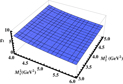
Figure 3: The strong coupling $g_{1}(Q^{2})$ as a function of the Borel parameters $\mathbf{M}^{2}=(M_{1}^{2},\ M_{2}^{2})$ at the fixed $(s_{0},s_{0}^{\prime})=(21,7)~{}\mathrm{GeV}^{2}$ and $Q^{2}=5~{}\mathrm{GeV}^{2}$.

The extracted strong coupling $g_{1}(Q^{2})$ depends on $\mathbf{M}^{2}$ and $\mathbf{s}_{0}$; the working intervals for these parameters are chosen in such a way as to minimize these uncertainties. For an example, in Fig. 3, we plot the coupling $g_{1}(Q^{2})$ as a function of the Borel parameters $M_{1}^{2}$ and $M_{2}^{2}$. It is seen that the changing of $\mathbf{M}^{2}$ leads to varying of the coupling $g_{1}(Q^{2})$, which nevertheless remains within allowed limits.

The width of the decay under analysis should be computed using the strong coupling at the $D^{+}$ meson’s mass shell $q^{2}=m_{D}^{2}$, which is not accessible to the sum rule calculations. We evade this difficulty by employing a fit function $F_{1}(Q^{2})$ that for the momenta $Q^{2}>0$ coincides with QCD sum rule’s predictions, but can be extrapolated to the region of $Q^{2}<0$ to find $g_{1}(-m_{D}^{2})$. In the present work, to construct the fit function $F_{1}(Q^{2})$, we use the analytic form

$$F_{i}(Q^{2})=F_{0}^{i}\mathrm{\exp}\left[c_{1}^{i}\frac{Q^{2}}{m_{T}^{2}}+c_{2}^{i}\left(\frac{Q^{2}}{m_{T}^{2}}\right)^{2}\right],$$ (30)

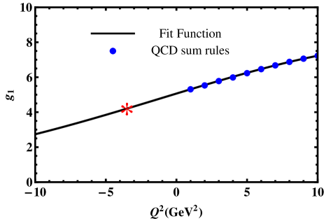
Figure 4: The sum rule predictions and fit function for the strong coupling $g_{1}(Q^{2})$. The star shows the point $Q^{2}=-m_{D}^{2}$.

where $F_{0}^{i}$, $c_{1}^{i}$ and $c_{2}^{i}$ are fitting parameters. Numerical analysis allows us to fix $F_{0}^{1}=5.06$, $c_{1}^{1}=0.83$ and $c_{2}^{1}=-0.38$. In Fig. 4 we depict the sum rule predictions for $g_{1}(Q^{2})$ and also provide $F_{1}(Q^{2})$; a nice agreement between them is evident.

This function at the mass shell $Q^{2}=-m_{D}^{2}$ gives

$$g_{1}\equiv F_{1}(-m_{D}^{2})=4.21\pm 0.65.$$ (31)

The width of decay $T\rightarrow D^{+}D^{\ast}(2007)^{0}$ is determined by the simple formula

$$\Gamma\left[T\rightarrow D^{+}D^{\ast}(2007)^{0}\right]=\frac{g_{1}^{2}\lambda^{3}\left(m_{T},m_{1D^{\ast}},m_{D}\right)}{8\pi m_{1D^{\ast}}^{2}},$$ (32)

where

$$\lambda\left(a,b,c\right)=\frac{1}{2a}\sqrt{a^{4}+b^{4}+c^{4}-2\left(a^{2}b^{2}+a^{2}c^{2}+b^{2}c^{2}\right)}.$$ (33)

Using the strong coupling from Eq. (31), it is not difficult to evaluate width of the decay$T\rightarrow D^{+}D^{\ast}(2007)^{0}$

$$\Gamma\left[T\rightarrow D^{+}D^{\ast}(2007)^{0}\right]=(64.3\pm 16.5)\ \mathrm{MeV}\text{.}$$ (34)

The second process $T\rightarrow D^{0}D^{\ast}(2010)^{+}$ can be considered via the same manner. Corrections which should to be made in the physical side and matrix elements of the previous decay channel are trivial.  Thus, the QCD side of the new sum rule in the approximation $m_{u}=m_{d}=0$ adopted in this paper coincides with $\Pi_{\mu}^{\mathrm{OPE}}(p,p^{\prime})$. The Borel and threshold parameters $\mathbf{M}^{2}$ and $\mathbf{s}_{0}$ are chosen as in the first process. The differences are connected with the spectroscopic parameters of produced mesons $D^{0}$ and $D^{\ast}(2010)^{+}$. These factors modify numerical predictions for $g_{2}(Q^{2})$, which is the strong coupling of the vertex $TD^{0}D^{\ast}(2010)^{+}$, and change the fit function $F_{2}(Q^{2})$. For parameters of $F_{2}(Q^{2})$, we get $F_{0}^{2}=5.11$, $c_{1}^{2}=0.83$, and $c_{2}^{2}=-0.38$. The result for the partial width of the decay $T\rightarrow D^{0}D^{\ast}(2010)^{+}$ reads

$$\Gamma\left[T\rightarrow D^{0}D^{\ast}(2010)^{+}\right]=(65.6\pm 16.8)\ \mathrm{MeV}\text{.}$$ (35)

The decay of the scalar four-quark meson $\widetilde{T}\rightarrow D^{+}D^{0}$ is the last process to be considered in this section. To extract the sum rule for the strong coupling $G(q^{2})$ corresponding to the vertex $\widetilde{T}D^{+}D^{0}$ we start from the correlation function,

$$\widetilde{\Pi}(p,p^{\prime})=i^{2}\int d^{4}xd^{4}ye^{i(p^{\prime}y-px)}\langle 0|\mathcal{T}\{J^{D}(y)$$

$$\times J^{D^{0}}(0)\widetilde{J}^{\dagger}(x)\}|0\rangle,$$ (36)

where $\widetilde{J}(x)$ and $J^{D}(x)$ are the interpolating currents of the particles $\widetilde{T}$ and $D^{+}$ defined by Eqs. (2) and (21), respectively. For the interpolating current of the pseudoscalar meson $D^{0}$, we use

$$J^{D^{0}}(x)=\overline{u}^{j}(x)i\gamma_{5}c^{j}(x).$$ (37)

Then, it is not difficult to get the physical side of the sum rule

$$\widetilde{\Pi}^{\mathrm{Phys}}(p,p^{\prime})=\frac{\langle 0|J^{D}|D^{+}(p^{\prime})\rangle\langle 0|J^{D^{0}}|D^{0}(q)\rangle}{(p^{\prime 2}-m_{D}^{2})(q^{2}-m_{D^{0}}^{2})}$$

$$\times\frac{\langle D^{0}(q)D^{+}(p^{\prime})|\widetilde{T}(p)\rangle\langle\widetilde{T}(p)|\widetilde{J}^{\dagger}|0\rangle}{(p^{2}-m_{\widetilde{T}}^{2})}+\ldots$$ (38)

Introducing the new matrix elements

$$\langle 0|J^{D^{0}}|D^{0}(q)=\frac{m_{D^{0}}^{2}f_{D^{0}}}{m_{c}},$$

$$\langle D^{0}(q)D^{+}(p^{\prime})|\widetilde{T}(p)\rangle=G(q^{2})(p\cdot p^{\prime}),$$ (39)

one can rewrite $\widetilde{\Pi}^{\mathrm{Phys}}(p,p^{\prime})$ in terms of the physical parameters

$$\widetilde{\Pi}^{\mathrm{Phys}}(p,p^{\prime})=G(q^{2})\frac{m_{D}^{2}f_{D}f_{\widetilde{T}}m_{\widetilde{T}}}{2m_{c}^{2}(p^{\prime 2}-m_{D}^{2})(p^{2}-m_{\widetilde{T}}^{2})}$$

$$\times\frac{m_{D^{0}}^{2}f_{D^{0}}}{(q^{2}-m_{D^{0}}^{2})}\left(m_{\widetilde{T}}^{2}+m_{D}^{2}-q^{2}\right)+\ldots$$ (40)

In Eqs. (39) and (40), $m_{D^{0}}$ and $f_{D^{0}}$ are the $D^{0}$ meson’s mass and decay constant, respectively.

The QCD side of the sum rule $\widetilde{\Pi}^{\mathrm{OPE}}(p,p^{\prime})$ is given by the expression

$$\widetilde{\Pi}^{\mathrm{OPE}}(p,p^{\prime})=i^{2}\int d^{4}xd^{4}ye^{i(p^{\prime}y-px)}\epsilon\widetilde{\epsilon}\left\{\mathrm{Tr}\left[\gamma_{5}S_{c}^{ic}(y-x)\right.\right.$$

$$\left.\times\gamma_{\mu}\widetilde{S}_{c}^{ib}(-x)\gamma_{5}\widetilde{S}_{u}^{dj}(x)\gamma^{\mu}S_{d}^{ei}(x-y)\right]-\mathrm{Tr}\left[\gamma_{5}S_{c}^{ib}(y-x)\right.$$

$$\left.\left.\times\gamma_{\mu}\widetilde{S}_{c}^{jc}(-x)\gamma_{5}\widetilde{S}_{u}^{dj}(x)\gamma^{\mu}S_{d}^{ei}(x-y)\right]\right\}.$$ (41)

The standard operations with $\widetilde{\Pi}^{\mathrm{Phys}}(p,p^{\prime})$ and $\widetilde{\Pi}^{\mathrm{OPE}}(p,p^{\prime})$ yield the sum rule

$$G(q^{2})=\frac{2m_{c}^{2}}{m_{D}^{2}f_{D}f_{\widetilde{T}}m_{\widetilde{T}}m_{D^{0}}^{2}f_{D^{0}}}\frac{q^{2}-m_{D^{0}}^{2}}{m_{\widetilde{T}}^{2}+m_{D}^{2}-q^{2}}$$

$$\times e^{m_{\widetilde{T}}^{2}/M_{1}^{2}}e^{m_{D}^{2}/M_{2}^{2}}\widetilde{\Pi}(\mathbf{M}^{2},\mathbf{\ s}_{0},~{}q^{2}).$$ (42)

In numerical calculations, the auxiliary parameters for the $\widetilde{T}$ and $D^{+}$ channels are chosen as in Eqs. (18) and (29), respectively. The parameters of the fit function $F_{3}(Q^{2})$ are equal to $F_{0}^{3}=0.31~{}\mathrm{MeV}^{-1}$, $c_{1}^{3}=-1.15$, and $c_{2}^{3}=0.92$, which at the mass shell $Q^{2}=-m_{D^{0}}^{2}$ leads to the strong coupling

$$G\left(-m_{D^{0}}^{2}\right)=(0.43\pm 0.07)\ \mathrm{GeV}^{-1}.$$ (43)

The width of this decay is determined by the expression

$$\Gamma[\widetilde{T}\rightarrow D^{+}D^{0}]=\frac{G^{2}m_{D}^{2}}{8\pi}\lambda\left(1+\frac{\lambda^{2}}{m_{D}^{2}}\right),$$ (44)

where $\lambda=\left(m_{\widetilde{T}},m_{D},m_{D^{0}}\right)$. Numerical computations predict

$$\Gamma[\widetilde{T}\rightarrow D^{+}D^{0}]=(12.4\pm 3.1)\ \mathrm{MeV}\text{.}$$ (45)

Parameters	Values ( $\mathrm{MeV}$ )
$m_{D^{0}}$	$1864.83\pm 0.05$
$m_{D}$	$1869.65\pm 0.05$
$m_{1D^{*}}~{}(D^{*}(2007)^{0})$	$2006.85\pm 0.05$
$m_{2D^{*}}~{}(D^{*}(2010)^{+})$	$2010.26\pm 0.05$
$f_{D}$	$203.7\pm 1.1$
$f_{D^{*}}$	$263\pm 21$

Table 1: Parameters of $D$ mesons produced in the decays of the tetraquarks $T$ and $\widetilde{T}$.

The partial width of these decays are the main result of the present section.

IV Conclusions

In this work we have explored features of the double-charmed pseudoscalar and scalar tetraquarks $T$ and $\widetilde{T}$. We have calculated their masses and couplings as well as found partial width of their strong decays. Our result for $m_{T}$ has allowed us to interpret the resonance $T$ as a member of the multiplet of double-charmed pseudoscalar tetraquarks. Saturating the full width of $T$ by the decays $T\rightarrow D^{+}D^{\ast}(2007)^{0}$ and $T\rightarrow D^{0}D^{\ast}(2010)^{+}$, it is possible to find

$$\Gamma_{T}=(129.9\pm 23.5)~{}\mathrm{MeV}.$$ (46)

Other members of this multiplet are tetraquarks $T_{cc;\overline{s}\overline{s}}^{++}$ and $T_{cc;\overline{d}\overline{s}}^{++}$, which were explored in Ref. Agaev:2018vag . These tetraquarks together with $T$ form the correct pattern of the pseudoscalar multiplet. Indeed, masses of these particles differ from each other by  approximately $125~{}\mathrm{MeV}$, caused by an existence or absence of $s$ quark(s) in their contents. The full widths of the exotic mesons $\Gamma[T_{cc;\overline{s}\overline{s}}^{++}]=(302~{}\pm 113)~{}\mathrm{MeV}$ and $\Gamma[T_{cc;\overline{d}\overline{s}}^{++}]=(171~{}\pm 52)~{}\mathrm{MeV}$ are large, and we can classify them as broad resonances. The full width of the tetraquark $T$ differs from $\Gamma[T_{cc;\overline{s}\overline{s}}^{++}]$ considerably but is comparable to $\Gamma[T_{cc;\overline{d}\overline{s}}^{++}]$. Therefore, we include the pseudoscalar tetraquark $T$  in a class of broad resonances.

The scalar double-charmed tetraquark $\widetilde{T}$ with full width $\Gamma_{\widetilde{T}}=(12.4\pm 3.1)~{}\mathrm{MeV}$ is a relatively narrow state. This resonance is a member of a double-charmed scalar tetraquarks’ multiplet. Investigation of other members of this multiplet, calculation of their masses, and partial and full widths can provide valuable information about properties of these scalar particles.

References

- (1) J. P. Ader, J. M. Richard and P. Taxil, Phys. Rev. D 25, 2370 (1982).
- (2) H. J. Lipkin, Phys. Lett. B 172, 242 (1986).
- (3) S. Zouzou, B. Silvestre-Brac, C. Gignoux, and J. M. Richard, Z. Phys. C 30, 457 (1986).
- (4) J. Carlson, L. Heller, and J. A. Tjon, Phys. Rev. D 37, 744 (1988).
- (5) S. Pepin, F. Stancu, M. Genovese, and J. M. Richard, Phys. Lett. B 393, 119 (1997).
- (6) Y. Cui, X. L. Chen, W. Z. Deng, and S. L. Zhu, High Energy Phys. Nucl. Phys. 31, 7 (2007).
- (7) J. Vijande, A. Valcarce, and K. Tsushima, Phys. Rev. D 74, 054018 (2006).
- (8) D. Ebert, R. N. Faustov, V. O. Galkin, and W. Lucha, Phys. Rev. D 76, 114015 (2007).
- (9) J. Schaffner-Bielich, and A. P. Vischer, Phys. Rev. D 57, 4142 (1998).
- (10) A. Del Fabbro, D. Janc, M. Rosina, and D. Treleani, Phys. Rev. D 71, 014008 (2005).
- (11) S. H. Lee, S. Yasui, W. Liu, and C. M. Ko, Eur. Phys. J. C 54, 259 (2008).
- (12) T. Hyodo, Y. R. Liu, M. Oka, K. Sudoh, and S. Yasui, Phys. Lett. B 721, 56 (2013).
- (13) A. Esposito, M. Papinutto, A. Pilloni, A. D. Polosa, and N. Tantalo, Phys. Rev. D 88, 054029 (2013).
- (14) F. S. Navarra, M. Nielsen, and S. H. Lee, Phys. Lett. B 649, 166 (2007).
- (15) M. L. Du, W. Chen, X. L. Chen, and S. L. Zhu, Phys. Rev. D 87, 014003 (2013).
- (16) R. Aaij et al. [LHCb Collaboration], Phys. Rev. Lett. 119, 112001 (2017).
- (17) M. Karliner and J. L. Rosner, Phys. Rev. Lett. 119, 202001 (2017).
- (18) E. J. Eichten, and C. Quigg, Phys. Rev. Lett. 119, 202002 (2017).
- (19) S. S. Agaev, K. Azizi, B. Barsbay, and H. Sundu, Phys. Rev. D 99, 033002 (2019).
- (20) S. S. Agaev, K. Azizi, B. Barsbay, and H. Sundu, Nucl. Phys. B 939, 130 (2019).
- (21) Z. G. Wang, and Z. H. Yan, Eur. Phys. J. C 78, 19 (2018).
- (22) T. Hyodo, Y. R. Liu, M. Oka, and S. Yasui, arXiv:1708.05169.
- (23) X. Yan, B. Zhong, and R. Zhu, Int. J. Mod. Phys. A 33, 1850096 (2018).
- (24) S. Q. Luo, K. Chen, X. Liu, Y. R. Liu, and S. L. Zhu, Eur. Phys. J. C 77, 709 (2017).
- (25) A. Ali, A. Y. Parkhomenko, Q. Qin and W. Wang, Phys. Lett. B 782, 412 (2018).
- (26) Y. Kondo, O. Morimatsu, and T. Nishikawa, Phys. Lett. B 611, 93 (2005).
- (27) S. H. Lee, H. Kim, and Y. Kwon, Phys. Lett. B 609, 252 (2005).
- (28) Z. G. Wang, Int. J. Mod. Phys. A 30, 1550168 (2015).
- (29) H. Sundu, S. S. Agaev, and K. Azizi, Eur. Phys. J. C 79, 215 (2019).
- (30) H. Sundu, B. Barsbay, S. S. Agaev, and K. Azizi, Eur. Phys. J. A 54, 124 (2018).
- (31) M. Tanabashi et al. (Particle Data Group), Phys. Rev. D 98, 030001 (2018).
- (32) D. Ebert, R. N. Faustov, and V. O. Galkin, Phys. Lett. B 635, 93 (2006).
- (33) A. Bazavov et al. [Fermilab Lattice and MILC Collaborations], Phys. Rev. D 85, 114506 (2012).
- (34) P. Gelhausen, A. Khodjamirian, A. A. Pivovarov, and D. Rosenthal, Phys. Rev. D 88, 014015 (2013) Erratum: [Phys. Rev. D 89, 099901 (2014)] Erratum: [Phys. Rev. D 91, 099901 (2015)].
- (35) Z. G. Wang, Eur. Phys. J. C 75, 427 (2015).
- (36) N. Dhiman, and H. Dahiya, Eur. Phys. J. Plus 133, 134 (2018).