Developmental trajectory of Caenorhabditis elegans nervous system governs its structural organization

Abstract

A central problem of neuroscience involves uncovering the principles governing the organization of nervous systems which ensure robustness in brain development. The nematode Caenorhabditis elegans provides us with a model organism for studying this question. In this paper, we focus on the invariant connection structure and spatial arrangement of the neurons comprising the somatic neuronal network of this organism to understand the key developmental constraints underlying its design. We observe that neurons with certain shared characteristics - such as, neural process lengths, birth time cohort, lineage and bilateral symmetry - exhibit a preference for connecting to each other. Recognizing the existence of such homophily helps in connecting the physical location and morphology of neurons with the topological organization of the network. Further, the functional identities of neurons appear to dictate the temporal hierarchy of their appearance during the course of development. Providing crucial insights into principles that may be common across many organisms, our study shows how the trajectory in the developmental landscape constrains the eventual spatial and network topological organization of a nervous system.

I Introduction

The presence of an efficient machinery for responding immediately to changes in the environment with appropriate actions is essential for the survival of any organism. In almost all multicellular animals, this role is played by the nervous system comprising networks of neurons, specialized cells that rapidly exchange signals with a high degree of accuracy. It allows information about the environment obtained via sensory receptors to be processed and translated into output signals conveyed to effectors such as muscle cells. In even the simplest of such organisms, the structural description of the interconnections between neurons provided by the connectome presents an extremely complicated picture Lichtman et al. (2014). How the complex organization of the nervous system is generated in the course of development of an organism, occasionally referred to as the “brain wiring problem” Hassan and Hiesinger (2015), is one of the most challenging questions in biology Mitchell (2007); Adolphs (2015). Only over the past few decades is the intricate interplay of different developmental phenomena, including cellular differentiation, migration, axon guidance and synapse formation, responsible for the formation of the network, being gradually revealed Araújo and Tear (2003); Chen and Cheng (2009); Colón-Ramos (2009); Kolodkin and Tessier-Lavigne (2011); Kaiser (2017).

The free-living nematode Caenorhabditis elegans, the only organism whose entire connectome has been reconstructed so far White et al. (1986); Varshney et al. (2011), is the natural choice for a system in which to look for principles governing the development of complexity in the nervous system Brenner (2009). The nervous system of the mature hermaphrodite individuals of the species comprises $302$ neurons, which is about a third of the total complement of $959$ somatic cells in the animal. Their lineage, positions in the body of the worm and connections to each other appear to be almost invariant across individuals White et al. (1986); Riddle et al. (1997). The small number of cells constituting the worm has made it a relatively tractable system for understanding the genetic basis of metazoan development and behavior. This, however, belies the sophistication of the organism which exhibits almost all the important specialized tissue types that occur in larger, more complex animals, prompting it to be dubbed as a “microchip animal” Haag et al. (2018). The availability of its complete genome sequence Hillier et al. (2005) along with detailed information about the cell lineage Sulston and Horvitz (1977); Sulston et al. (1983) means that, in principle, the developmental program can be understood as a consequence of genetically-encoded instructions and self-organized emergence arising from interactions between diverse molecules and cells Emmons (2016).

The “wiring problem” for the C. elegans nervous system had been posed early on with Brenner essentially raising the following questions: how are the neurons spatially localized in their specific positions, how they connect to each other through synapses and gap junctions forming a network with a precisely delineated connection topology, and what governs the temporal sequence in which different neurons appear over the course of development Brenner (1974). Subsequent work have identified several mechanisms underlying the guidance of specific axons and formation of synapses between particular neurons Culotti (1994); Margeta et al. (2008); Cherra and Jin (2015). However, the minutiae of the diverse molecular processes at work may be too overwhelming for us to arrive at a comprehensive understanding of how the complexity manifest in the nervous system of the worm arises. Indeed, it is not even clear that all the guidance cues that are involved in organizing the wiring are known Goodhill (2016). An analogous situation had prevailed five decades earlier when C. elegans had been first pressed into service to understand how genetic mutations lead to changes in behavior of an organism. Brenner had responded to this challenge by analyzing the system at a level intermediate between genes and behavior Brenner (1974). Thus, the problem was decomposed into trying to understand (a) the means by which genes specify the nervous system (how is it built ?) and (b) the way behavior is produced by the activity of the nervous system (how does it work ?) Brenner (1974); Emmons (2016). In a similar spirit, for a resolution of the “wiring problem”, we may need to view it at a level intermediate between the detailed molecular machinery involving diffusible factors, contact mediated interactions, growth cone guidance, etc., and the organization of the neuronal network in the mature worm. Specifically, in this paper, we have focused on uncovering a set of guiding principles that appear to govern the neuronal wiring and spatial localization of cell bodies, and which are implemented by the molecular mechanisms mentioned earlier (and thus genetically encoded). From the perspective of the three-level framework proposed by Marr Marr (1982) for understanding the brain Adolphs (2015), viz., comprising (i) computational (or functional), (ii) algorithmic and (iii) implementation levels, such principles can be viewed as algorithms for achieving specific network designs realized over the course of development Hassan and Hiesinger (2015).

For this purpose, we have used the analytical framework of graph theory, which has been successfully applied to understand various aspects of brain structure and function, in both healthy and pathological conditions Bassett et al. (2008); Bullmore and Sporns (2009); Park and Friston (2013); Stam (2014); Fornito et al. (2015); Schröter et al. (2017). For the specific case of the C. elegans nematode, application of such tools has revealed the existence of network motifs Reigl et al. (2004), hierarchical structure Chatterjee and Sinha (2007), community (or modular) organization Pan et al. (2010) and a rich club of highly connected neurons Towlson et al. (2013). Comparatively fewer studies have focused on the evolution of the network during development of the nematode nervous system that we consider here Varier and Kaiser (2011); Alicea (2018). We have integrated information about spatial location of cells, their lineage, time of appearance, neurite lengths and network connectivity to understand how its developmental history constrains the design of the somatic nervous system of C. elegans, specifically the $279$ connected neurons which control all activity of the worm except the pharyngeal movements. Thus, our study complements existing work that has focused more on understanding the structural organization of the network using efficiency and optimality criteria such as minimization of the wiring cost, delineated by the physical distance between neurons Ahn et al. (2006); Chen et al. (2006); Pérez-Escudero and de Polavieja (2007); Rivera-Alba et al. (2014); Gushchin and Tang (2015); Wang and Clandinin (2016).

The key questions related to development that we address here involve the spatial location of the cell bodies (why is the neuron where it is, relative to other neurons ?), the temporal sequence in which the cells appear (why is it that certain neurons are born much earlier than others ?) and the topological arrangement of their inter-connections (why does a neuron have the links it does ?). As reported in detail below, we find that these questions are related to the existence of general principles that can be expressed in terms of different types of homophily, the tendency of entities sharing a certain feature to preferentially connect to each other. We discern four different types of homophily, involving respectively, process or neurite length of neurons, the time of their appearance, their lineage history and bilateral symmetry. Our results help reveal that the ganglia, anatomically distinct bundles into which the neurons are clustered in the nematode, are formed of several groups (or families) of cells, neurons within each group being closely related.

At a higher level of network organization, we show that neurons which play a vital role in coordinating activity spanning large distances across the network by connecting together distinct neuronal clusters also appear quite early in the sequence of development. This observation (along with others, such as linking the functional type of neurons, viz., sensory, motor and inter, to their time of appearance) helps link the situation of a specific cell in the temporal hierarchy to which all neurons belong, with its function. We also provide an analysis of the inter-relation between functional, structural and developmental aspects, focusing on neurons identified to belong to different functional circuits, such as those associated with mechanosensation Chalfie et al. (1985); Wicks and Rankin (1995); Sawin (1996), chemosensation Troemel et al. (1997), etc. This provides us with a more nuanced understanding of the relation between the time of appearance of a neuron and the number of its connections. Our results suggest that developmental history plays a critical role in regulating the connectivity and spatial localization of neurons in the C. elegans nervous system. In other words, development itself provides key constraints on the system design. In addition, the tools we employ here for revealing patterns hidden in the lineage and connectivity information, including novel visual representations of developmental history, such as chrono-dendrograms, provide insights into principles governing the wiring of nervous systems that may be common across several organisms.

II Results

II.1 Homophily based on multiple cellular properties governs neuronal inter-connectivity

Direct contact between neurons whose cell bodies are located relatively far apart, through synapses or gap junctions located on their extended processes, plays a crucial role in reducing communication delay of signals across the entire nervous system Kaiser and Hilgetag (2006). This is particularly relevant for C. elegans where the majority of synapses occur en passant (forming at axonal swellings) between parallel nerve process shafts that can remain close to each other over long distances Riddle et al. (1997). Therefore, in order to understand the principles governing the wiring organization of the nematode nervous system, it is appropriate to first focus on understanding how the connectivity of neurons is influenced by the length of their neurites.

It has also been observed that connected pairs of neurons very often differentiate close to each other in time Varier and Kaiser (2011). This may suggest that preferential connectivity among neurons according to the time of their birth (i.e., birth cohort homophily) is a possible basis for guiding the network architecture. However, we need to explore the possibility that it could be a consequence of the restrictions on connections between neurons imposed by their respective process lengths. For instance, a large majority of the neurons that are born early, i.e., prior to hatching, are localized in the head region and have short processes extending to less than a third of the body length of the nematode. This could, in principle, be sufficient to explain the temporal closeness of connected neurons. We have accordingly investigated the joint dependence of the occurrence of connections between neurons on the lengths $\ell$ of their respective processes, as well as, their birth times $t_{b}$ in Fig. 1 (A-B). The distance $d$ between the cell bodies for each pair of connected neurons is also indicated, which makes apparent the restriction on connectivity imposed by the process lengths. This information adds a temporal dimension to our understanding of the organization of long-range connections (corresponding to high values of $d$) in the nematode nervous system. An entry (colored point) in the $i$-th row and $j$-th column of the matrices shown in Fig. 1 (A) and (B), corresponds to a chemical synapse or electrical gap junction [for (A) and (B), respectively] from neuron $j$ to neuron $i$ ($i,j=1,\ldots,225$ being the indices referring to each of the neurons in the C. elegans nervous system whose process length is known). The color represents the distance $d$ between cell bodies as per the adjoining color bar. The neurons (indicated along the rows and columns) are grouped according to their process lengths $\ell$. These are categorized as short ($\ell\leq L/3$), medium ($L/3<\ell\leq 2L/3$) and long ($\ell>2L/3$) relative to the total body length of the worm $L$. Moreover, within each category, the neurons are arranged by their time of birth in increasing order.

Process length homophily. Even a perfunctory perusal of the two matrices makes it apparent that the diagonal blocks in the two matrices, corresponding to connections between neurons having similar process length, have a relatively higher density of points. This observation indicates that there is a preponderance of connections within each group characterized by how far their neurites extend. However, to establish that there is indeed process length homophily which would imply, for instance, that neurons with short processes tend to prefer connecting to other neurons having short processes, we will have to compare the empirically observed number of such connected pairs with that expected to arise by chance given the degree (i.e., the total number of connections) of each neuron.

To quantitatively estimate the bias that neurons may have in connecting to neurons with similar neurite lengths, we cluster the cells into three communities or modules which are characterized by all their members having short, medium or long processes, respectively. This allows us to calculate the modularity $Q$, a measure of the extent to which like prefers connecting to like in a network Newman, Mark E.J. (2004); Newman (2010) (see Methods for details). Low values of $Q(\sim 0)$ would indicate that there is no evidence to support homophily, while a relatively large positive value for a particular module would suggest that there is a bias for its members to preferentially connect to each other. To see whether this is statistically significant we compare the empirical value of $Q$ with that for an ensemble of randomized surrogates. We compute the latter from $10^{3}$ networks, each constructed from the empirical adjacency matrix (either synaptic or gap-junctional) by randomly permuting the membership of the neurons to the three communities characterized by the process lengths (long, medium and short) of their members.

For the entire synaptic network, we measure the empirical value of $Q$ to be $0.117$, while for the network of neurons connected by gap junctions, it is $0.134$. Both of these values are significantly higher than the corresponding values for the randomized surrogates, viz., $-0.002\pm 0.010$ for the synaptic and $-0.004\pm 0.020$ for the gap-junctional networks, respectively. This suggests that neurons having similar process lengths do indeed have many more of their connections with each other than would be expected simply on the basis of the number of synapses and gap junctions possessed by each of them. Individually considering the three communities, comprising neurons having short, medium and long processes, respectively, also yields $Q$ that differ significantly from the corresponding randomized surrogates (see Supplementary Material, Table S1). Thus, although the empirical values of the modularity appear to be small, they cannot be attributed simply to fluctuations resulting from the small numbers involved and suggests the existence of specific mechanisms that make connections between two neurons, both of which have short (or long) processes, more likely.

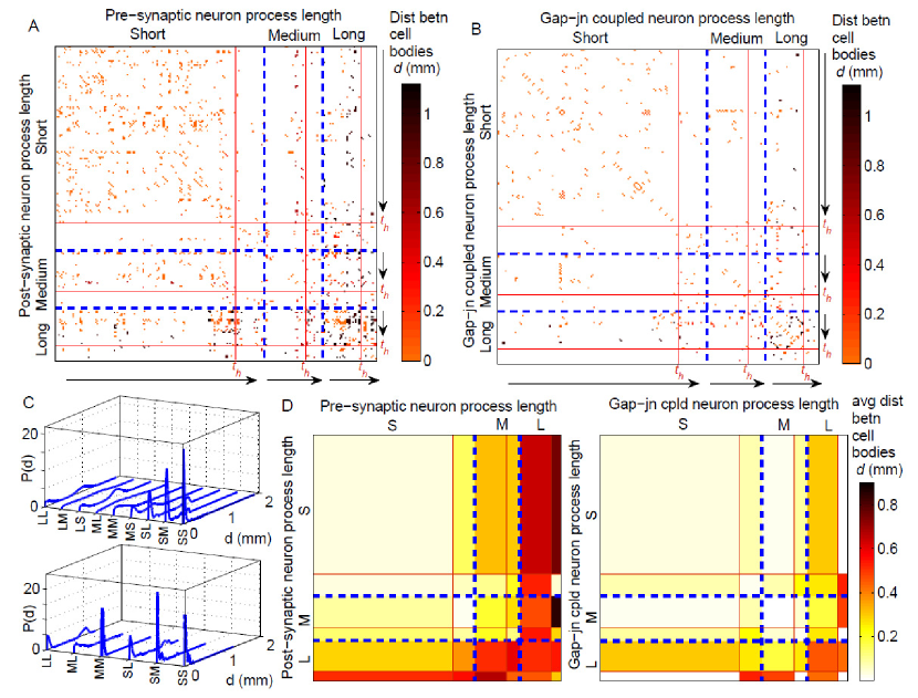
Figure 1: Birth time cohort membership and neurite lengths of neurons govern their connectivity. (A-B) Matrices representing synaptic (A) and gap-junctional (B) connections that exist between neurons, grouped into three classes [indicated by blue broken lines] according to their process lengths $\ell$ measured relative to the worm body length $L$, viz., short ($\ell\leq L/3$), medium ($L/3<\ell\leq 2L/3$) and long ($\ell>2L/3$), and ordered within each class according to birth time. Increasing birth time is indicated by arrows, with red lines marked $t_{h}$ (time of hatching) separating neurons which differentiate in the embryonic stage from those born later. Matrix entries correspond to the existence of a connection, with its color representing the distance (measured in mm) between cell bodies of the corresponding neurons (see legend). We observe that there is evidence of birth time assortative mixing, with neurons born early(later) having a higher probability of connecting with other early(late) born neurons, which is particularly marked in the case of neurons having short processes. The gap junction matrix shows a large number of entries adjacent to the diagonal which correspond to connections between paired neurons [see Fig. 5 (A)]. (C) Distribution of distances $d$ between cell bodies of pairs of neurons distinguished in terms of their respective process lengths (S: short, M: medium, L: long), which are connected by synapses (top) and gap junctions (bottom). As synaptic connections are directed, there are nine possible combinations of pairs of the classes (S/M/L) to which the pre- and post-synaptic neurons belong (e.g., SL refers to a synapse from a neuron with a short process to a long process length neuron). On the other hand, as gap junctions are undirected, only six possible combinations need be considered. We note the bimodal distributions of $d$ when at least one of the two neurons connected by synapse or gap junction has a long (or medium) process. (D) The mean distance $\langle d\rangle$ between cell bodies of neurons connected by synapses (left) and gap junctions (right), grouped according to their process lengths (L/M/S) [indicated by blue broken lines] and further subdivided into those born early (i.e., embryonic stage) and those born late (i.e., L1, L2 or L3 stages) [separated by red lines]. Distances are expressed in mm (see legend for the color code). We note that pre-synaptic neurons with long processes tend to connect with post-synaptic neurons having short processes which are located far from them, corresponding to the higher peak in the bimodal distribution for LS in top panel of (C). Note that we have considered in this analysis the subset of 225 neurons for which information about process length is available.

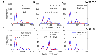
Figure S1: Birth cohort homophily is seen specifically for connections between neurons whose cell bodies are in close physical proximity. Frequency distributions of the mean birth time for all pairs that are connected via synapses (A-C) or gap-junctions (D-F). The distributions for the empirical network (shown in red) are compared with distributions obtained from surrogate ensembles of randomized networks (blue curve shows the average over $100$ realizations, the dispersion being indicated by the shaded area). The latter are constructed from the empirical network by randomly rewiring the connections while keeping the total number of connections (degree) for each neuron, the spatial location of its cell body and its process length unchanged. In addition, to allow only physically possible connections between neurons, we have imposed process-length constraint which disallow linking two cells if the distance between their cell bodies is greater than the sum of their individual process lengths. The different panels correspond to connections between neurons whose cell bodies are separated by distance $d$ which is short ($d<L/3$: A, D), medium ($L/3<d<2L/3$: B, E) or long ($d>2L/3$: C, F) relative to the total body length of the worm $L$. As in Fig. 4 in the main text, the trimodal nature of these distributions arise from three classes of connected neuronal pairs, viz., (i) where both cells are born early (i.e., in the embryonic stage), (ii) where one is born early while the other late (i.e., in the post-embryonic stage) and (iii) where both are born late. Birth cohort homophily is indicated when the peaks of the empirical frequency distribution, corresponding to connections between neurons that are either both born early or both born late, have significantly higher values than the randomized distribution (the latter corresponding to a null model where connections between cells can occur independent of the time of their birth). This is seen only in panels (A) and (D), i.e., for connections between neurons whose cell bodies are located relatively close to each other.

We observe a relatively high density of points in Fig. 1 (A and B) in the blocks corresponding to cells having short processes that are born at the same epoch, i.e., either pre- or post-hatching. We also see this in the block in panel (A) corresponding to connections between pre-synaptic neurons with short processes and post-synaptic neurons with medium process length. This suggests that, apart from process length, the time of birth of the cells also determine neuronal inter-connectivity. Indeed, earlier studies Varier and Kaiser (2011) have shown that most of the neurons that are connected to each other happen to be born close in time, with the probability of connection between almost contemporaneous neurons being much more than what is expected by chance. However, we find that the actual temporal separation between the time of birth of different neurons does not have any significant correlation (viz., $p\gg 0.05$) with the probability of there being a connection between them, either synaptic or gap-junctional. This apparent contradiction is resolved on noting the following. While, within the group of neurons born in the embryonic stage and those born post-embryonic, there may be a great diversity in terms of birth times (thereby significantly weakening any correlation with connection probability), these differences are minor when viewed from the perspective of membership in the cohorts of those born pre- and post-hatching, respectively. As mentioned later, these correspond to two distinct, temporally separated bursts of neuronal differentiation, which provides a natural demarcation of the neurons into early and late-born categories. Moreover, this birth cohort homophily is specific to neurons whose cell bodies are located in close physical proximity (see Supplementary Material, Fig. S1). By comparing with randomized surrogates, we observe that connections between neurons are not significantly enhanced if they are born in the same epoch except for the case when the distance $d$ between their cell bodies is short ($d<L/3$).

So far, in our consideration of how connections between neurons is affected by their process lengths, we have not considered the information concerning the spatial position of the cell bodies of the connected neurons. Consideration of this information is important if we want to understand how activity of spatially distant parts of the organism are coordinated through long-range connections that allow signals to be rapidly transmitted across relatively large physical distances. Figs. 1 (C) and (D) show how the distance $d$ between cell bodies of connected pairs of neurons are distributed differently according to their respective process lengths.

The top panel in Fig. 1 (C) corresponds to the probability distribution function of distance between cell bodies $d$ for neurons connected by synapses, while the bottom panel considers gap junctions. When both the pre- and post-synaptic neurons have short processes (indicated by SS in the figure), it is expected that the cell bodies will be located close to each other. This is indeed what is observed, with a prominent peak of $P(d)$ occurring at extremely low values of $d$. On the other hand, when at least one of the neurons have a long or medium length process, we observe that the distributions for neurons connected through synapse are much more extended towards higher values. For SL, LS and LL connections, we in fact observed a distinct bimodal character in the corresponding distribution of $d$. This can be linked to the observation that neurons having short as well as long processes tend to predominantly have their cell bodies located at the head or in the tail of the worm. In contrast, neurons whose processes are intermediate in length have cell bodies distributed relatively more homogeneously across the body of the organism (see Supplementary Material, Fig. S2). This can be quantified by measuring the extent to which the cell bodies themselves are distributed along the longitudinal axis of the nematode body in a bimodal manner using the Bimodality Coefficient $(BC)$ metric Pfister et al. (2013) (see Methods). A distribution is said to be prominently bimodal if its $BC\gg BC^{*}$ ($=5/9$), the value of the metric for an uniform distribution. We find that while the spatial positions of the cell bodies of neurons having short, as well as, long process are distributed in a bimodal manner ($BC_{S}=0.93$ and $BC_{L}=0.83$, respectively), that of neurons with intermediate length process ($BC_{M}=0.67$) are relatively more uniformly distributed. Accordingly, we observe that synaptically connected pairs, in which at least one neuron has process of medium length, exhibit distributions of $d$ where bimodality is either muted (as in SM and MS) or absent (MM, ML and LM), even though all of these distributions span a much larger range than that of SS. This indicates that process length is an important determinative factor for the occurrence of long-range connections in the nematode nervous system.

When we consider the distribution of distances between cell bodies of neurons connected by gap junctions [lower panel of Fig. 1 (C)], we observe that connections are more likely to occur between spatially adjacent cell bodies. This is manifest in the distributions of $d$ being much less extended than those seen in the case of synapses, with the exception of SL and LL which exhibit bimodality. The distinction between the situations seen in the upper and lower panels may arise from the fact that while synapses between two neurons can in principle be located anywhere on their processes, gap junctions predominantly occur close to the cell body of at least one of the participating neurons. The greater importance of relative spatial positions of neurons in determining the occurrence of a gap junction is manifested in terms of a stronger (anti-) correlation between $d$ for a neuronal pair and the probability that they are connected by a gap junction, in comparison to a synapse (discussed later).

The detailed nature of the information about the number of neuronal pairs with given process lengths whose cell bodies are placed a specific distance $d$ apart that is provided by the distributions shown in Fig. 1 (C) tends to obscure certain gross features. The latter can impart important insights into how process length facilitates connections between spatially distal neurons. Therefore, in Fig. 1 (D) we display the average physical distance between cell bodies of connected neurons which are distinguished in terms of their process lengths (short/medium/long), and further subdivided into those appearing in the embryonic stage, i.e., prior to hatching (referred to as early), and those which appear at the post-embryonic stage (referred to as late). For synaptic connections (shown at left), the average $d$ for neurons with long processes (pre-synaptic) connected to neurons having short processes (post-synaptic) is the highest ($\langle d_{LS}\rangle=0.61$ mm) of all the categories considered, higher even than that when both neurons in a connected pair have long processes ($\langle d_{LL}\rangle=0.51$ mm). Intriguingly, both of these values are larger than the average distance between cell bodies for connected neurons when the pre-synaptic neurons have short processes while the post-synaptic ones have long processes, viz, ($\langle d_{SL}\rangle=0.32$ mm). This is consistent with the two peaks of the bimodal distribution of $d$ corresponding to these connections differing substantially in amplitude - the peak at lower $d$ being higher for SL, while the one at higher $d$ being larger for LS. To a lesser extent, a similar asymmetry is seen for the average distance between connected cell bodies when one has short process while the process of the other is of medium length (viz., $\langle d_{MS}\rangle=0.27$ mm as compared to $\langle d_{SM}\rangle=0.09$ mm).

We can compare these values with the average distance between cell bodies of all neurons, whether connected or not. For instance, the mean separation $D$ between cell bodies of all neurons with long process lengths is $\langle D\rangle_{L,L}=0.55$ mm which is almost the same as the average distance between every pair of neurons in which one has a short process and the other has a long one ($\langle D\rangle_{L,S}=0.54$ mm). To ensure that the difference between $\langle d_{XY}\rangle$ and $\langle D\rangle_{X,Y}$ (where $X,Y\in\{S,L,M\}$) is statistically significant, we show that it is extremely unlikely that the observed values of $d$ will arise by chance if random surrogates are constructed having the same number of connected neurons as is observed empirically (by sampling the set of all neuronal pairs without replacement). For instance, the $z$-score (see Methods) for the distance between cell bodies of pre-synaptic neurons with long processes connected to post-synaptic neurons with short processes is $z_{LS}=1.8$. By contrast, considering the reverse, i.e., synapses from neurons with short processes to those having long processes, we obtain $z_{SL}=-7.2$. Thus, neurons with long processes appear to form a synapse with neurons having short processes whose cell bodies are located far away from their own much more often than that expected by chance given the spatial positions of the cell bodies. On the other hand, neurons with short processes prefer to connect to neurons with long processes whose cell bodies are much closer to their own. Indeed, excepting the class of LS synaptically connected neuron pairs (i.e., pre-synaptic neuron having long process, post-synaptic neuron having short process) all other connected neural pair classes, distinguished in terms of the process lengths of the two neurons, have negative values for $z$-score (see Supplementary Material, Table S2). The results indicate that the process length of the pre-synaptic neuron is a dominant influence deciding the average distance between cell bodies connected by synapses. It is also consistent with the possibility that a high proportion of synaptic contacts are occurring close to the cell body of the post-synaptic neuron (which is closer to the classical concept of the pre-synaptic axon connecting to a dendrite close to cell body of the post-synaptic neuron and not just making a synaptic contact anywhere on the process). Such asymmetry between LS and SL may also have the advantage of functional efficiency in that the resulting connection architecture allows signals to rapidly travel large distances across the nematode body through long processes - thereby spreading globally using L to S connections - and then being disseminated locally using neurons with short processes.

If we now consider the case of neurons connected by gap-junctions [Fig. 1 (D, right)], we note that the average value of $d$ is highest for the case of cells with long processes connecting to each other. In particular, unlike the situation seen above for synaptically connected neurons, $\langle d_{LS}\rangle(=0.3$ mm) is lower than $\langle d_{LL}\rangle(=0.44$ mm). The $z$-score for the distance between cell bodies of neuron pairs whose members belong to any of the classes S,M and L are seen to be strongly negative, ranging between $z_{LL}=-2.2$ and $z_{SS}=-6.5$. The high statistical significance of $\langle d\rangle$ when compared against the average separation between neurons $\langle D\rangle$ suggests that gap junctions occur between neurons whose cell bodies lie close to each other far more often than expected by chance (given their positions). This is consistent with the belief that gap junctions predominantly act to coordinate activity locally between neurons Xu et al. (2018). As alluded to above, the larger magnitude of the $z$-score values for gap junctions as compared to synapses could possibly indicate that these junctions tend to form much closer to the cell body than the en passant synapses that can form at many different locations on the extended process of a neuron. We also note in passing another feature of gap junctional connections between neurons which is manifest in Fig. 1 (B) as a large number of entries in the adjacency matrix immediately neighboring the diagonal. These correspond to a very high proportion of connections between bilaterally symmetric pair of neurons, e.g., AVAL and AVAR, that is discussed later (see Fig. 5). These connections may have the possible functional goal of coordinating response of the nematode nervous system to sensory inputs between the left and right sides of the body Hall (2017).

The process length homophily between neurons that we report here can be attributed to multiple possible factors. For instance, the preference of neurons having long process for connecting to other neurons with long processes could be an outcome of the geometry resulting from parallel fibers extending over relatively large distances, which have a proportionately higher probability of forming en passant synapses with each other. On the other hand, the preference of neurons having short processes to connect to each other could be tied to the fact that many of their cell bodies are located in close physical proximity. This suggests an important role for the physical distance $d$ between cell bodies in deciding connectivity between neurons. For gap junctions, we do indeed observe a significant correlation of $-0.66$ ($p=0.001$) between $d$ and the probability that cells are connected [consistent with the high proportion of gap junctions occurring between neurons having cell bodies close to each other, see Fig. 1 (C), bottom]. However, for synapses, the relation between the two is less clear as the correlation is not statistically significant.

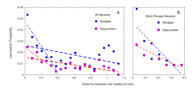
Figure S3: Dependence of the probability of connection between two neurons on the physical distance between their cell bodies. (A) The variation of the probability of connection between two neurons by either synapse (squares) or gap-junction (circles) as a function of the physical distance between their cell bodies $d$ (measured in mm). Linear fitting of the functions show a decay with $d$ overall (thick broken lines), but the relation is much weaker compared to that seen between probability of synaptic connection between two cells and their lineage distance $l$ [see Fig. 2 (D) in main text]. In particular, the correlation is diluted by the relatively high probability for synapses to form between neurons whose cell bodies are located at the opposite ends of the worm (corresponding to the peak around $x=1$ mm). However, when we focus only on connections between cell bodies that are in close physical proximity ($d<0.4$ mm), the dependence on $d$ appears to be much more prominent (thin broken lines). This stronger correlation between connection probability and $d$ at short distances is not necessarily an outcome of constraints imposed by the process lengths of the neurons. This is suggested by panel (B), where we focus exclusively on neurons with short processes. (B) The relation between connection probability between neurons, both of which have short processes, and the distance between their cell bodies, $d$, is seen to be not more prominent than that already seen for all neurons [in panel (A)].

Focusing only on neuron pairs whose cell bodies are located close to each other (i.e., $d\leq L/3$ where $L$ is the total body length of the worm), however, we observe a very strong correlation of $-0.94$ ($p=0.002$) between $d$ and the probability of a synaptic connection between the two (for gap junctions, the correlation is $-0.91$ with $p=0.004$). This high value indicates that synapse formation between neurons whose cell bodies are located near each other is indeed strongly dependent on the distance between them. Moreover, it cannot be explained in terms of simple physical limits imposed by the process lengths of neurons on the farthest distance allowed between cell bodies of connected neurons. This is because if we consider the correlation between $d$ and probability of connection only between neurons having short processes, we obtain a value of $-0.84$ ($p=0.02$) for synapses and $-0.83$ ($p=0.02$) for gap junctions (see Supplementary Material, Fig. S3).

A possible explanation for the weakening of the relation between connection probability and the physical distance separating the cell bodies when all neurons are considered could be because, even though neurons born in close physical proximity have a higher probability of getting connected, it is masked by the cells moving apart subsequently over the course of development. In the absence of information about the location of the cell bodies at the time synaptogenesis happens, we can probe this indirectly by considering how the probability of connection between two cells depends on how closely they are related in terms of lineage - as cells having common ancestry also tend to be born adjacent to each other.

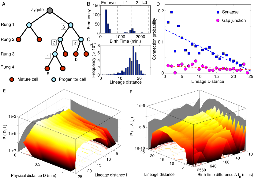
Figure 2: Lineage of neurons affects their synaptic connectivity and spatial localization. (A) Schematic diagram of a lineage tree of cells resulting from consecutive mitotic divisions of the zygote. The terminal nodes of the tree correspond to terminally differentiated mature cells (shown in red) while other nodes represent progenitors (shown in blue) that appear at different rounds of cell division. Cells born at each round of cell division are indicated by the corresponding rung of the tree they belong to, the numerical value for the rung (shown at the left) being the number of divisions starting from the zygote. The lineage distance $l$ between a pair of mature cells is measured as the total number of cell divisions leading to each from their common progenitor. An example of lineage distance measurement is shown in the figure for the pair of cells $a$ and $b$ which are separated by four cell divisions (the distance of $a$ from each of the intermediate dividing progenitors is indicated in the figure). (B-C) Frequency distributions of the birth time of different neurons (B, separated into the different developmental stages) and the lineage distances for each pair of neurons (C). (D) The probability of a pair of neurons to be connected through a synapse decreases with increasing lineage distance between them, as indicated by a statistically significant linear correlation between the two ($r=-0.86$, $p<10^{-7}$). In contrast, there is no significant variation of the probability of gap junctional connection with lineage distance. (E-F) Joint probability distributions of lineage distance $l$ along with distance between cell bodies $D$ (E) and birth time difference $\Delta t_{b}$ (F) between all pairs of neurons. The marginal distributions for the corresponding quantities are indicated in the bounding surfaces. Contours for the distributions are indicated at the base of each figure. We notice that the distribution of physical distances in (E) exhibit a bimodal nature. However, cells which are closely related in terms of lineage ($l<5$) also has a high probability of being physically located nearby (indicated by a prominent peak at the lower end of the distribution of $D$) which suggests that lineage influences spatial localization of cells. In panel (F), the distribution shows peaks at odd values of the lineage distance (particularly for low $\Delta t_{b}$) suggesting that neurons born close in time are located at the same rung on the lineage tree.

Lineage relation between neurons constrains the distance between their cell bodies, as well as, the likelihood of a synaptic connection between them. Cell lineage provides knowledge of the developmental trajectory in all metazoa, being defined by successive divisions starting from the zygote to the final differentiated cell. In most animals, the identity of any terminal node of the lineage tree, known as cell fate, is determined by intrinsic and extrinsic factors, as well as, interactions with neighboring cells. This introduces sufficient variability in the developmental path so as to make lineage relationships discernible only at the level of cell groups rather than individual cells Wood (1988). However, some organisms such as nematodes exhibit an almost invariant pattern of somatic cell divisions that is identical across individuals, and in the case of Caenorhabditis elegans, is known in its entirety Sulston and Horvitz (1977); Sulston et al. (1983). Thus, the lineage tree of the organism provides us with a complete fate map at single-cell resolution Giurumescu and Chisholm (2011). The schematic representation of such a tree shown in Fig. 2 (A) depicts successive mitotic cell divisions starting from a zygote that, through intermediate progenitor cells, eventually differentiate into mature neuronal cells. Each successive cell division (beginning from the zygote) corresponds to different rungs in the tree used to label the resulting daughter cells. The difference between any two cells in terms of their lineage can thus be quantified by their lineage distance, i.e., their separation on the tree measured as the total number of cell divisions that leads to each of them from their last common progenitor.

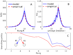
Figure S4: A stochastic branching model for the lineage tree of cells involved in the development of the C. elegans somatic nervous system. (A) Comparison of the distribution of rung $R$ occupied by each cell (progenitor cells of the neurons, as well as, differentiated neurons) in the lineage tree obtained empirically (broken curve) with that generated by the model (solid curve shows the mean computed over an ensemble of $10^{3}$ realizations, the dispersion being indicated by the shaded area). (B) Comparison of the distribution of lineage distance $l$ between pairs of differentiated neurons of C. elegans (broken curve) with that obtained from the model (solid curve showing the mean computed over an ensemble of $10^{3}$ realizations, the dispersion being indicated by the shaded area). The high degree of overlap between the empirical and simulated distributions indicates that the stochastic branching model is a reasonably accurate description of the lineage tree of neurons. (C) The branching probabilities $P1$ (blue curve) and $P2$ (red curve) of a progenitor cell at each rung, estimated from the empirical lineage tree (by definition, $P1\geq P2$). Note that both of the branching probabilities show a prominent dip after rung 10. Guided by this, in the stochastic branching model, $P1,P2$ have been chosen to have a constant high value upto rung 10 (viz., $P1=1$, $P2=0.85$), after which both are decreased to a constant low value (viz., $P1=0.25$, $P2=0.2$). The inset shows a schematic of the stochastic branching model where a node, occurring at any rung, can branch (or not) based on the probabilities $P1$ and $P2$ which will result in any one of the following three possibilities: (i) proliferation occurs along both branches, (ii) only one branch appears (the other branch leading to either apoptosis or a non-neural cell fate), and, (iii) there is no branching so that we obtain a terminal node of the tree (i.e., the cell differentiates into a neuron).

Apart from the lineage tree, crucial information on the relationships between different cells that stem from their developmental history is provided by the knowledge of birth times of the individual mature neurons, i.e., the specific instant in developmental chronology of the nervous system at which each neuron differentiates. Fig. 2 (B) shows the distribution of birth times for all cells belonging to the somatic nervous system of C. elegans, indicating that development of the system occurs in two bursts clearly separated in time. The ‘early burst’, during which the bulk, viz., 72%, of the neurons are born, occurs at the embryonic stage of development, while the more temporally extended ‘late burst’ spans across the L1 and L2 stages. This information, in conjunction with a simple generative model for reconstructing the lineage tree through successive cell divisions, can be used to explain the distribution of lineage distance shown in Fig. 2 (C). As at each node of the lineage tree a cell divides into at most two daughter cells, we can view it - at least in the first few rungs belonging to the early proliferative phase - as a balanced binary tree, with the number of cells that appear in each rung $R$ increasing exponentially with $R$ (upto $R=10$ in C. elegans, see Supplementary Material, Fig. S4). Within the AB sublineage of cells to which almost all the neurons belong, the maximum lineage distance that can occur between two cells which are placed in rungs $R_{1}$ and $R_{2}$, respectively, is given by $l_{max}(R_{1},R_{2})=(R_{1}-1)+(R_{2}-1)-1.$ Thus, the distribution of lineage distances has an exponential profile upto $l=17$. Beyond rung $10$, the subsequent branching of the nodes in the binary tree reduce markedly as many of the divisions terminate in differentiated neurons (and occasionally programmed cell death) or lead to non-neuronal fates (so that their further divisions are not considered for the purpose of this study). This can be seen to result in the lineage distance distribution decreasing exponentially for $l>17$, with a maximum lineage distance of $25$. A more detailed theoretical model of the lineage relationships between neurons resulting from their developmental history can be constructed as an asymmetric stochastic branching process (see Methods). Here, beginning with a single node that corresponds to the zygote, at each iteration every node that appeared during the preceding iteration is considered in turn for giving rise to each of two possible branches with probabilities $P1$ and $P2$ ($P1\geq P2$) that result in further nodes. By considering the actual lineage tree, these asymmetric branching probabilities in the model were fixed as $P1=1$ and $P2=0.85$ until rung 9 and for later rungs they were set to $P1=0.25$ and $P2=0.2$. For these values of $P1$ and $P2$, the trees generated by the model exhibited properties that were statistically similar to the empirical lineage tree (see Supplementary Material, Fig. S4).

Going back to the question we had posed earlier, viz., how does the lineage distance $l$ between cells affect the probability that they are connected by synapses, we observe from Fig. 2 (D) that there is indeed a strong correlation of $-0.86$ ($p<10^{-7}$) between the two. This observation provides evidence of lineage homophily being one of the key principles governing connectivity of the nematode nervous system. However, for gap junctions we do not see any significant relation between the probability of a connection between two neurons and how close they are in terms of their ancestry. These observations suggest the following plausible scenario, viz., synaptogenesis can occur early, just after neurons are born, while gap junctions are established much later during development, when neurons have more or less moved to their final positions. Thus, changes in the locations of cell bodies from that they occupied initially (i.e., at the time the corresponding neurons differentiated) which are brought about by the appearance of cells born later through subsequent cell-divisions, result in a weak correlation between synaptic connection probability and physical distance separating the cell bodies as alluded to earlier. It may also lead to neurons of dissimilar lineage (whose cell bodies need not initially be close) eventually move in physical proximity of each other allowing the possible formation of gap junctions between them.

The connection between lineage distance $l$ and physical distance $D$ between cell bodies of neurons (whether connected or not), which has been mentioned earlier, is illustrated by the joint probability distribution $P(D,l)$ shown in Fig. 2 (E). In particular, cells having short lineage distance, viz., $l\leq 5$, tend to have their cell bodies located close to each other, as indicated by the function being peaked towards lower values of $D$. However, cells that are farther apart in terms of lineage can occur at different distances from each other, resulting in the overall bimodal form for the marginal distribution of $D$. A similar nuanced relation between lineage distance for two neurons and the difference of the times $\Delta t_{b}$ in which they are born is indicated by the joint probability distribution $P(l,\Delta t_{b})$ shown in Fig. 2 (F). We note that for small $l$ ($l\leq 5$), the distribution peaks at low values of $\Delta t_{b}$ indicating that closely related neurons tend to be born within a short time interval of each other. We also observe that the distribution of $l$ between neurons that differentiate at around the same time (i.e., for low $\Delta t_{b}$) tends to alternate between peaks and troughs for odd and even values, respectively. This is easy to explain if neurons that are contemporaneous occur at the same rung (as, by definition, neurons at the same rung will have odd values of lineage distance between themselves).

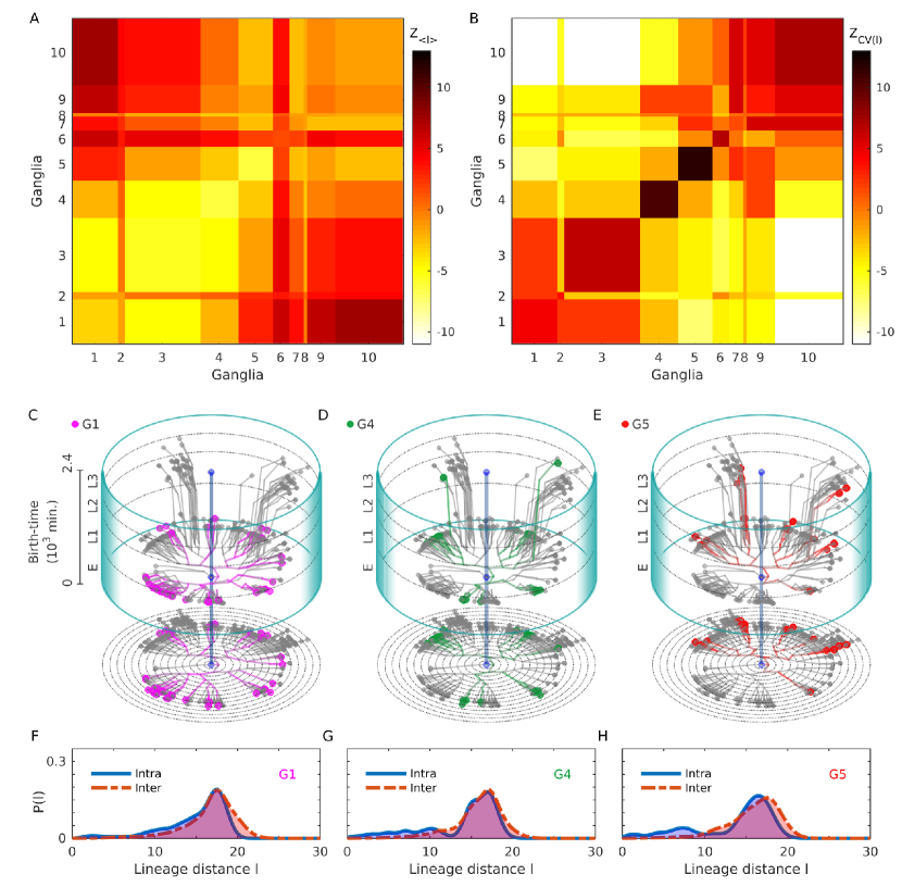
Figure 3: Lineage distance reveals developmental patterns of ganglia. (A-B) Statistically significant features of the distribution of intra and inter-ganglionic lineage distances, quantified by deviations of the mean $\langle l\rangle$ (A) and coefficient of variation $CV$ (B), from a surrogate ensemble of randomized lineage trees of neurons in the C. elegans somatic nervous system. These deviations (measured by $z$-score) show that the mean intra-ganglionic lineage distances (represented by diagonal blocks of the matrix) are significantly lower than that of the inter-ganglionic lineage distances (off-diagonal blocks). By contrast, CV for the intra-ganglionic lineage distances are significantly higher than that of the inter-ganglionic lineage distances. (C-E) Developmental chrono-dendrograms for three representative ganglia (viz., G1, G4 and G5) show that each comprises multiple localized clusters of neurons occurring at different locations on the developmental lineage tree, explaining the statistically significant deviations of the mean and CV for intra-ganglionic lineage distances. Colored nodes represent neurons belonging to the specified ganglion while grey nodes show the other neurons. Branching lines trace all cell divisions starting from the single cell zygote (located at the origin) and terminating at each differentiated neuron. The time and rung of each cell division is indicated by its position along the vertical and radial axis respectively. The entire time period is divided into four stages, viz., Embryo (indicated as E), L1, L2 and L3. A planar projection at the base of each cylinder shows the rung (concentric circles) of each progenitor cell and differentiated neuron. (F-H) The probability distribution functions for the intra-ganglionic lineage distances show bimodality (unlike that of the inter-ganglionic distances), which is consistent with the segregation of a ganglion into multiple clusters along the chrono-dendrogram. The different ganglia are indicated by symbols G1-G9 (1: Anterior, 2: Dorsal, 3: Lateral, 4: Ventral, 5: Retrovesicular, 6: Posterolateral, 7: Preanal, 8: Dorsorectal and 9: Lumbar) and the Ventral cord as G10.

The different ganglia comprise clusters of closely related neurons. The compelling association between lineage and physical proximity of neurons alluded to above is manifest in the spatial organization of the cell body locations. It is particularly conspicuous in the clustering of neurons into anatomically distinct bundles that are referred to as ganglia. These structures, characteristic of nematode nervous systems, contain only cell bodies of the neurons with their axonal and dendritic processes located outside of the bundles Schafer (2016). The somatic nervous system comprises nine such spatially localized clusters, viz., anterior, dorsal, lateral, ventral, retrovesicular, posterolateral, preanal, dorsorectal and lumbar ganglia, with the remainder belonging to the ventral cord. Comparison of the distributions of intra-ganglionic lineage distances (i.e., between pairs of neurons located in the same ganglion) with that of inter-ganglionic lineage distances (i.e., between neurons in different ganglia) provides an insight into how these bundles can be interpreted from a developmental perspective.

We first note that the mean of the lineage distances $\langle l\rangle$ within a given ganglia are typically much smaller than those between different ganglia. Moreover, as seen from Fig. 3 (A), the mean of the intra-ganglionic lineage distances for most ganglia are significantly small, which we determine by comparing with values of $\langle l\rangle$ obtained from ensembles of $10^{3}$ surrogate lineage trees where the identity of each of the leaf nodes (i.e., the differentiated neurons) has been randomly permuted. This randomization decouples the ganglionic membership of the neurons from their position on the lineage tree while keeping the lineage distances between cells invariant, consistent with our null hypothesis that the ganglion to which a neuron belongs is independent of its developmental history. The observed mean intra-ganglionic lineage distances deviate markedly from those obtained from the surrogate trees (as measured by $z$-score, see Methods), indicating that neurons in a ganglion are much more closely related to each other than expected by chance.

However, when we consider the coefficient of variation ($CV$), a relative measure of the dispersion in the lineage distances within a ganglion or between two ganglia, we note that this is almost always greater for intra-ganglionic, compared to the inter-ganglionic, lineage distances [Fig. 3 (B)]. We can again establish the statistical significance by measuring the same quantities for the ensemble of surrogate lineage trees mentioned above and quantifying the difference between the actual tree and the randomized ensemble using $z$-scores. The large values of $z$ for CV in most of the diagonal blocks (corresponding to intra-ganglion dispersion) shown in Fig. 3 (B), suggests that the relatedness between neurons in a ganglion shows a much larger variability than expected by chance.

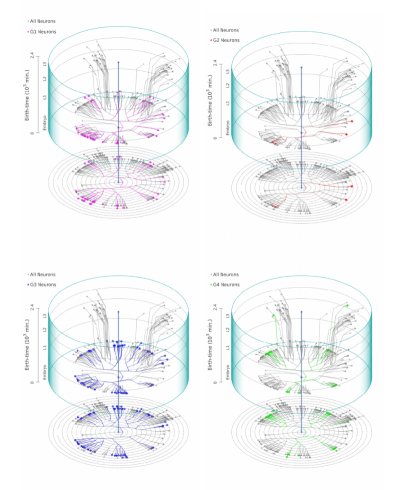
Figure S5: Developmental chrono-dendrograms for the Anterior (G1, top left), Dorsal (G2, top right), Lateral (G3, bottom left) and Ventral (G4, bottom right) ganglia, showing that each comprises multiple localized clusters of neurons. Colored nodes represent neurons belonging to the specified ganglion while grey nodes show other neurons. Branching lines trace all cell divisions starting from the single cell zygote (located at the origin) and terminating at each differentiated neuron. The time and rung of each cell division is indicated by its position along the vertical and radial axis respectively. The entire time period is divided into four stages, viz., Embryo (indicated as E), L1, L2 and L3. A planar projection at the base of each cylinder shows the rung (concentric circles) of each progenitor cell and differentiated neuron.

The apparent contradiction between the results mentioned above, viz., that a majority of the neurons in a ganglion have a shared lineage while, at the same time, exhibit a high degree of diversity in their lineage relations, is easily resolved on inspecting the chrono-dendrograms that visually represent the complete developmental trajectory for each of the ganglia [shown in Fig. 3 (C-E), for the anterior, ventral and retrovesicular ganglia; see Supplementary Material, Figs. S5-S7 for the others]. While the lineage tree shown in each of these figures is, of course, identical, the neurons that belong to a particular ganglion are distinguished (by color) in the corresponding chrono-dendrogram, allowing us to note at a glance how all the members of the given ganglion relate to each other. We note that the differentiated neurons that constitute a ganglion are typically organized into multiple clusters, each of which are highly localized on the lineage tree. In other words, a ganglion comprises several ‘families’ of neurons emanating from different branches of the tree, with each family composed of closely related cells sharing a last common ancestor separated from them by only a few cell divisions.

The grouping of the cells belonging to a particular ganglion into distinct clusters, which are widely separated on the lineage tree, is reflected in the bimodal nature of the distribution of intra-ganglionic lineage distances [Fig. 3 (F-H)]. In contrast to the unimodal distribution seen for inter-ganglionic lineage distances, the neurons within a ganglion could either have (i) extremely low distances to cells which belong to their own ‘family’ or (ii) large distances to cells belonging to the other ‘families’ that constitute the ganglion. These manifest, respectively, as a smaller peak at lower values and a larger peak at higher values of $l$ seen in Fig. 3 (F-H). The bimodality gives rise to a large dispersion and hence a value for the CV of lineage distances that is higher than expected. Note that the peak at higher $l$ for this distribution almost coincides with the peak of the inter-ganglionic $l$ distribution, which is expected as the latter is dominated by cells that are not closely related. Thus, the presence of the second peak at lower values of $l$ in the intra-ganglionic distribution reduces the mean lineage distance for cells within a ganglion, compared to that for cells belonging to different ganglia. Conversely, the absence of multiple peaks in the inter-ganglionic distribution provides for a smaller value of the CV compared to the case for the intra-ganglionic distribution. Thus, these results explain the apparently contradictory coexistence of low mean value and high CV for lineage distances of neurons within a ganglion, which is related to the localization of the developmental trajectories of cells belonging to it into distinct groups visible in the lineage tree. This clearly demonstrates that the spatial segregation of neurons into ganglia is shaped by the relations between the constituent cells which arise from their shared developmental history.

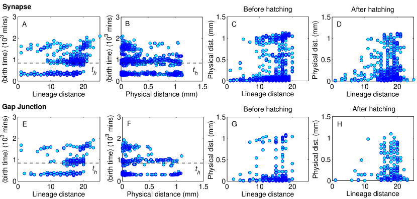
Figure 4: Birth times and lineage distances constrain connections between neurons whose cell bodies are spatially distant from each other. (A-B) The mean birth time of synaptically connected pairs of neurons exhibit a trimodal distribution, with connections clustering into three temporal groups corresponding to those (i) between neurons that are both born early, i.e., in the embryonic stage, (ii) between one born early and the other born late (i.e., in the post-embryonic stage), and (iii) between neurons that are both born late. The hatching time $h_{t}$ separating the embryonic from other developmental stages is indicated by the broken line. We note from panel (B) that when both neurons are born late (corresponding to the uppermost cluster of connections), synaptic connections are more likely to occur between neurons whose cell bodies are located close to each other. (C-D) Synaptic connections between neurons that are closely related to each other in terms of lineage ($l<10$) occur almost always when their cell bodies are in proximity, regardless of the time of birth of the neurons. We note that this restriction is more pronounced than observed in Fig. 2 (E), where $P(D,l)$ shows a prominent peak at the lower end of $D$ for small $l$ suggesting that most closely related neurons (whether connected or not) typically have short distances between their cell bodies. (E-H) Neurons connected by gap junctions show patterns similar to those seen in the case of synaptic connections.

Connected neurons. Having considered the distribution of physical distance, lineage distance and birth-time differences between all neuronal pairs in the somatic nervous system, we now focus on the subset of connected pairs to see how the above factors may constrain the probability that a neuron has a direct interaction with another. Fig. 4 shows the inter-relations between similarity of ancestry, spatial separation and birth times for each pair of neurons that are linked either by synapses (top row) or gap junctions (bottom row). The clustering of mean birth times of the connected pairs into three distinct groups (seen in panels A-B and E-F) is a consequence of the two bursts of neuronal differentiation widely separated in time [seen in Fig. 2 (B)]. Thus, the lower and upper clusters correspond to connected neurons both of which appear in the course of the same developmental burst (early and late, respectively), while connections between neurons that arose during different bursts populate the intermediate cluster.

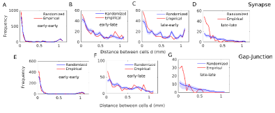
Figure S8: Connections between neurons born at different developmental epochs are over-represented when the cell bodies are far apart, suggesting the presence of active processes facilitating such links. Frequency distributions of the distance $d$ between cell bodies of all neuronal pairs that are connected via synapses (A-D) or gap-junctions (E-G). The distributions for the empirical network (shown in red) are compared with distributions obtained from surrogate ensembles of randomized networks (blue curve shows the average over $100$ realizations, the dispersion being indicated by the shaded area). The latter are constructed from the empirical network by randomly rewiring the connections while keeping the total number of connections (degree) for each neuron, the spatial location of its cell body and its process length unchanged. In addition, to allow only physically possible connections between neurons, we have imposed process-length constraint which disallow linking two cells if the distance between their cell bodies is greater than the sum of their individual process lengths. The different panels correspond to the situations where (A,E) both cells in a connected pair are born in the early developmental burst, (B,C,F) one is born early and the other is born late [in (B) it is the pre-synaptic neuron which is born early, while in (C) the post-synaptic neurons appears in the early developmental burst], and (D,G) both cells are born late. When two neurons are born in the same developmental epoch (either early or late), the empirical frequency distribution is seen to have significantly higher values than the randomized distribution at low $d$ (seen in panels A and D, and even more prominently in panels E and G), indicating that neurons prefer to connect to other members of their birth cohort whose cell bodies are in close proximity. This is particularly evident for neurons born in the late developmental epoch. Note that this result complements the earlier observation that birth cohort homophily is seen specifically for neurons whose cell bodies are located relatively close to each other (Fig. S1). More intriguingly, connections between neurons whose cell bodies lie far apart are seen to occur more frequently than expected by chance when the pre-synaptic neuron is born early and the post-synaptic neuron is born late (see panel B). A similar phenomenon is also seen in the case of early- and late-born neurons connected by gap junctions (see panel F). These results suggest the presence of an active process forming connections between neurons born in different epochs.

In Fig. 2 (F) we had already seen that closely related neurons tend to have similar birth times. This helps explain why, as seen in Fig. 4 (A), whenever synaptically connected neurons have short lineage distance to each other, they also happen to belong to the same developmental burst epoch. However, apart from the relative differences in the birth times, the actual time of differentiation also determines the occurrence of a synapse between neurons. Indeed, it is known from Ref. Varier and Kaiser (2011) that about 68% of long-range synaptic connections occur between neurons both of which are born in the early burst of neuronal differentiation. This is complemented by Fig. 4 (B) which shows that synapses between neurons, whose cell bodies are separated by large distances, mostly occur when at least one of the neurons was born early. Conversely, when both neurons are born in the late burst, such long-range links become extremely unlikely. Indeed, the distribution of distances between cell bodies of connected neurons (see Supplementary Material, Fig. S8, that compares the empirical data with degree-preserved randomized networks where the connections are made according to constraints imposed by the length of processes of each neuron) show that long-range connections in the nematode typically do not occur significantly more often than that expected by chance, given the process lengths of the neurons. Thus, specific mechanisms for explaining the occurrence of such connections maybe unnecessary given that en passant synaptic contacts form between neighboring parallel neuronal processes. In contrast, short range connections are much more numerous than that seen in the random surrogate networks. This suggests that active processes may be driving synaptogenesis Margeta et al. (2008); Cherra and Jin (2015) between neurons lying in close proximity, for example, chemoattractant diffusion Tessier-Lavigne and Goodman (1996); Chen and Cheng (2009); Kolodkin and Tessier-Lavigne (2011). Furthermore, the exceptional feature of early pre-synaptic neurons having long-range connections to late post-synaptic neurons much more often than is expected by chance could suggest a possible role of fasciculation in this process Kaiser (2017). For instance, late-born neurons could be following the extended processes of earlier neurons to connect to cell bodies placed far away.

In Fig. 4 (C) and (D) we compare explicitly the pre- and post-hatching scenarios in order to see whether early and late-born neurons differ in terms of how the synaptic connections between them are influenced by the lineage and/or physical distances between them. We note that for both groups of cells, closely related neurons that are connected by synapse also happen to occur at spatially proximate locations. This is consistent with Fig. 2 (E) where the peak in the joint probability distribution of all neuronal pairs with lineage distance $l$ and physical distance $D$ is observed to occur at low $D$ when $l$ is small. Qualitatively similar results are observed when we consider neuronal pairs connected by gap junctions [see panels E-H of Fig. 4].

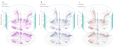
Figure S9: Absence of segregated clusters in the developmental chrono-dendrograms for neurons having similar process lengths (viz., short, medium and long) suggest that process length is not exclusively determined by lineage. Colored nodes represent neurons having a specified process length, viz., short in (A), medium in (B) and long in (C), while grey nodes show other neurons. Branching lines trace all cell divisions starting from the single cell zygote (located at the origin) and terminating at each differentiated neuron. The time and rung of each cell division is indicated by its position along the vertical and radial axis respectively. The entire time period is divided into four stages, viz., Embryo (indicated as E), L1, L2 and L3. A planar projection at the base of each cylinder shows the rung (concentric circles) of each progenitor cell and differentiated neuron.

The results reported above provide remarkable evidence for the role that developmental attributes (viz., lineage distances and birth-times of neurons) play in shaping the spatial organization of cell bodies and the topological structure of the connections in the somatic nervous system of the worm. However, the process length homophily described earlier appears to be independent and cannot be explained as a consequence of lineage homophily. The chrono-dendrograms (see Supplementary Material, Fig. S9) showing the positions of neurons with short, medium and long processes, respectively, on the lineage tree indicate that neurons having a particular process length do not cluster together. This suggests that neurons with extremely similar lineage may have very different process lengths (and vice versa), so that the observed bias in the connection probability between neurons having processes of similar length cannot simply be attributed to a common lineage.

Bilaterally symmetric neurons. The major fraction ($\approx 66\%$) of neurons belonging to the somatic nervous system of C. elegans occur in pairs. These are located along the left and right sides of the body of the nematode in a bilaterally symmetric fashion. While there are instances of bilaterally symmetric neurons exhibiting functional lateralization (e.g., ASEL/R, see Ref. Hobert (2014)), the vast majority of the left/right members of such pairs remain in the symmetrical “ground state”, i.e., they are indistinguishable functionally, as well as, in terms of anatomical features and gene expression Hobert (2005). In particular, whenever one member of a bilaterally symmetric pair occurs in any of the known functional circuits, the other also appears in it without exception. While it is known that this symmetric nature is manifested in the spatial arrangement (e.g., location of the cell bodies) and connection structure of paired neurons, here we ask whether bilaterally symmetric neurons share a similar network neighborhood, i.e., whether there is a high degree of overlap between the neurons that each of them connect to, or indeed whether they have a significantly higher probability of being connected to each other. The latter assumes importance in view of the fact that it is the direct contact between the paired cells AWCL/R that trigger asymmetrical gene expression resulting in differential expression of olfactory-type G-protein coupled receptors in the neurons Hobert et al. (2002).

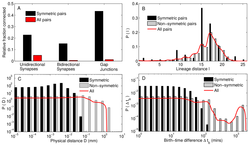
Figure 5: Symmetrically paired neurons have a high probability of being connected and also exhibit strong association in their birth times and spatial positions. (A) Bilaterally symmetric neurons that are positioned on the left and right of the body axis of the organism tend to have a much higher probability of synaptic, as well as, gap junctional connections between them, compared to that for all pairs of neurons. In addition, the synapses are highly likely to be reciprocal (bidirectional). (B) The distribution of lineage distances between paired neurons show that the mean value is lower than that for all neurons. We note that almost all lineage distances between symmetric neurons are odd-valued suggesting that they occur at the same rung of the lineage tree. (C-D) Symmetrically paired neurons have cell bodies located in physical proximity of each other (C) and are born close in time as indicated by low birth-time differences $\Delta t_{b}$ (D), compared to all pairs of neurons.

Fig. 5 (A) shows that indeed the left/right members of a symmetric pair have a much higher probability of connection between them than any two arbitrarily chosen neurons belonging to the somatic system. Moreover, $15\%$ of the bilaterally symmetric pairs have reciprocal synaptic connections with each other, compared to less than $1\%$ of all neuronal pairs being connected in such a bidirectional manner. We can further distinguish the symmetric neuron pairs into those which originate from an early division across left/right axis of the common ABp blastomere (i.e., they have similar lineage differing only in the early cell division event ABpl/r) and those where members of a pair originate from non-symmetric blastomeres (e.g., ABal and ABpr) Hobert (2014). These two distinct origins of the bilaterally symmetric neurons are reflected in the two peaks of the distribution of lineage distance between the left/right members of each pair seen in Fig. 5 (B), with only the latter category of paired neurons that do not share a bilaterally symmetric lineage history having low values of $l$. The synaptic connection probability between the members of pairs belonging to these two classes differ only by a small amount ($0.26$ for the former and $0.19$ for the latter, with the corresponding numbers reducing to 0.18 and 0.12, respectively, when we consider reciprocal synapses). The occurrence of gap junctions between bilaterally symmetric neurons is seen to be exceptionally high ($43\%$ of such pairs being connected) compared to that for the entire system, with no distinction in numbers being observed between the two categories of symmetric pairs. This preponderance of gap-junctional connections between bilaterally symmetric neurons (also indicated by the band diagonal structure of the connectivity matrix shown in panel (B) of Fig. 1) suggests that their activity is highly coordinated. This may possibly explain the co-occurrence of both members of a symmetric pair in the different functional circuits.

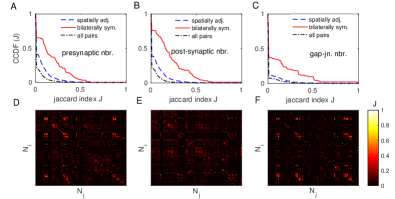
Figure S10: Physical proximity alone cannot explain the high degree of overlap between the cells that each member of a bilaterally symmetric pair of neurons connect to. Complementary cumulative probability distributions (CCDF) of the overlap between the sets $\mathcal{N}_{G}(i)$, $\mathcal{N}_{G}(j)$ of the neighbors (defined for a network $G$) of neurons $N_{i}$ and $N_{j}$, where the indices $i$ and $j$ can run over (i) all pairs of neurons (dash-dotted curves), (ii) only bilaterally symmetric pairs (solid curves) or (iii) pairs whose cell bodies are spatially adjacent to each other ($d<0.05$ mm, broken curves). The overlap is measured in terms of the Jaccard index $J$, defined for the pair $i,j$ as $J(i,j)=[\mathcal{N}_{G}(i)\cap\mathcal{N}_{G}(j)]/[\mathcal{N}_{G}(i)\cup\mathcal{N}_{G}(j)]$, where $\cap$ and $\cup$ refers to intersection and union of two sets, respectively. The different panels correspond to different networks $G$ used to define neighbors for a neuron, viz., (A) pre-synaptic neighbors, i.e., cells from which the neuron receives a synaptic connection, (B) post-synaptic neighbors, i.e., cells to which the neuron sends a synaptic connection, and (C) gap-junctional neighbors, i.e., cells to which a neuron is coupled via a gap junction. We note that the overlaps between the neighborhoods (for all three types of network neighbors considered here) of bilaterally symmetric neurons are consistently higher than that of all pairs of neurons, as well as, of pairs whose cell bodies are in close physical proximity. Thus, bilaterally symmetric neurons share neighbors to a much greater extent than that expected by their cell bodies being located close to each other. (D-F) The Jaccard index matrices $J$ showing overlaps between the neighbors for every pair of neurons $N_{i}$, $N_{j}$ when the network neighborhood defined is that of (D) pre-synaptic partners, (E) post-synaptic partners and (F) gap-junctional partners. The large overlap between neighbors of bilaterally symmetric neurons is indicated by the occurrence of bands of brightly colored entries along the diagonal (note that bilaterally symmetric neurons are always located on adjacent rows/columns).

In addition to exhibiting a high probability of being connected directly, bilaterally symmetric neurons are also characterized by a high degree of neighborhood similarity. Fig. S10 in Supplementary Material shows the magnitude of overlap between the neurons that each member of a pair is connected by a synapse (either pre- or post-synaptically) or a gap junction, which is seen to be much higher than that for any two arbitrarily chosen neurons. This is consistent with the left/right neurons in the majority of bilaterally symmetric pairs having an identical role in terms of the mesoscopic organization of the network (see discussion related to Fig. 7). The large number of neighbors that paired neurons share in common is a striking feature that cannot be explained from their physical proximity alone.

We note that almost all lineage distances between symmetric neurons are odd-valued suggesting that they are born at the same rung of the lineage tree. The only exception is the pair AVFL/R, whose members have distinct non-symmetric lineage history, with a lineage distance of 8. Given their shared lineage, it is perhaps unsurprising that most bilaterally symmetric paired neurons also exhibit strong associations in their physical locations and birth times. Panels (C-D) show that a large fraction of the left/right members have cell bodies that are located in close physical proximity of each other (C) and are also born close in time as indicated by low birth-time differences $\Delta t_{b}$ (D), compared to all pairs of somatic neurons. Indeed we note that the only exception is the late-born pair SDQL/R with bilaterally symmetric history whose members are located in the anterior and posterior (respectively) parts of the organism, the physical distance between the cell bodies being $0.5$ mm.

II.2 Temporal hierarchy of the appearance of neurons during development is associated with their functional identity

We have been focusing, so far, on the various properties related to the developmental history of neurons which govern their spatial organization as well as their inter-connectivity. The latter, as we have shown above, is guided by several types of homophily, i.e., the tendency of neurons which are similar in terms of certain features - viz., process length, lineage, birth-time and bilateral symmetry - to be connected via synapses or gap junctions. We shall now see how the functional identities of neurons are related to their developmental histories. In particular, we show that classes of neurons distinguished by their (i) functional identity (viz., sensory, motor and interneurons), (ii) functional role in the mesoscopic structural organization of the network and (iii) membership in distinct functional circuits, strongly influences the temporal order of their appearance in the developmental chronology of the nervous system.

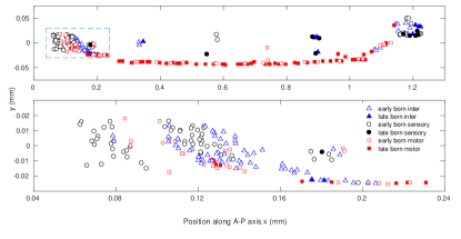
Figure S11: Spatial distribution of the cell bodies of sensory, inter and motor neurons of the somatic nervous system of Caenorhabditis elegans. Projections of the physical locations of the neuronal cell bodies, distinguished according to functional type (sensory: circles, inter: triangles and motor: squares) and whether they appear in the early (unfilled symbols) or late (filled symbols) developmental epochs, on the two-dimensional plane formed by the anterior-posterior (AP) axis ($x$, along the horizontal) and the dorsal-ventral axis ($y$, along the vertical). Top panel shows the entire worm, with its body oriented such that the head is located near the left end and tail near the right end of the plane. The bottom panel shows a magnified view of the region near the head (bounded by broken lines in the top panel). We note that almost all cells in this region appear at the embryonic stage, during the early burst of development. By contrast, the ventral cord predominantly comprises neurons that appear in the post-embryonic stage (see top panel).

Functional types. One of the simplest classifications of neurons is according to their position in the hierarchy along which signals travel in the nervous system. Thus, sensory neurons receive information from receptors located on the body surface of the organism and transmit them onward to interneurons, which allow signals arriving from different parts to be integrated, with appropriate response being eventually communicated to motor neurons that activate effectors such as muscle cells. In the mature C. elegans somatic nervous system, the motor neurons form the majority ($106$), while sensory ($77$) and interneurons ($83$) are comparable in number. The remaining neurons are polymodal and cannot be uniquely assigned to a specific functional type. In Fig. 6 (A) we show how the sub-populations corresponding to each of the distinct functional types evolve over the course of development of the organism. We immediately note that while the bulk of the sensory and interneurons differentiate early, i.e., in the embryonic stage, followed by a more gradual appearance of the few remaining ones in the larval stages, more than half of the motor neurons appear much later after hatching. Moreover, of the $48$ motor neurons which appear early, approximately half ($23$) belong to the nerve ring while the rest are in the ventral cord, where they almost exclusively innervate dorsal muscles (the positions of neurons, classified according to function type and birth time, is shown in Supplementary Material, Fig. S11). On the other hand, the $58$ late-born motor neurons primarily belong to the ventral cord (with only $4$ appearing in the nerve ring). In addition, the majority of them ($41$) innervate ventral body muscles (see Supplementary Table LABEL:T3 for details). The few ($11$) late-born motor neurons that do innervate dorsal muscles differ from the early-born ones in that they do not have complementary partners and bring about asymmetric muscle activation Tolstenkov et al. (2018). This early innervation of dorsal muscle but late, larval-stage innervation of ventral muscles could embody developmental constraints that deserve further exploration in the future.

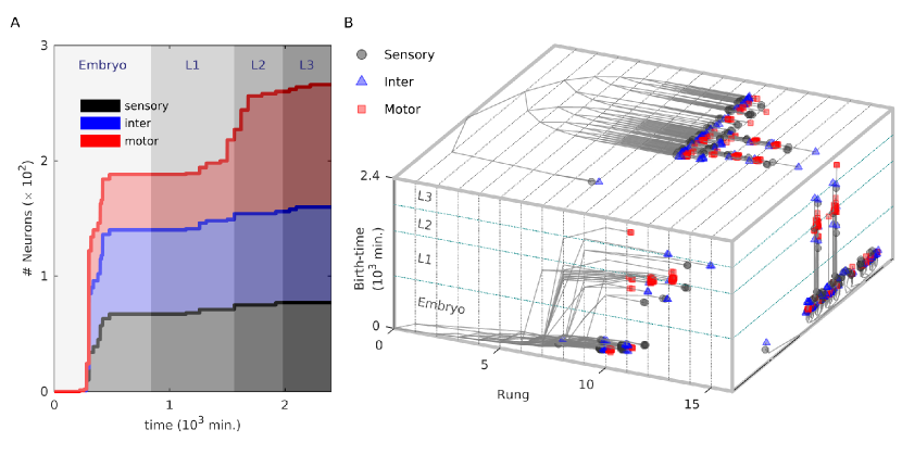
Figure 6: Developmental histories of neurons show a bifurcation into early and late branches, with a predominance of motor neurons in the latter. (A) Bulk of the sensory and interneurons appear early, i.e., during the embryonic stage, while a large fraction of motor neurons differentiate much later (L2 or L3) during development. (B) Planar projections of a three-dimensional representation of the developmental history of the entire somatic nervous system of C. elegans. Different colors and symbols have been used to denote distinct neuron types (viz., sensory, motor and interneurons). The projection on the top surface shows the lineage tree with branching lines connecting the single cell zygote (shown at rung 0) to each of the differentiated neurons located on their corresponding rungs. At higher rungs ($>11$) we see that the differentiated cells are tightly clustered into two bundles of branches with a predominance of motor neurons (also seen in the chrono-dendrogram projection shown at the right face of the base). We note the absence of segregated clusters comprising exclusively the same functional type of neurons (viz., sensory, motor or inter), suggesting that the progenitor cell can give rise to neurons of different types. This in turn implies that commitment to a particular neuron function occurs quite late in the sequence of cell divisions. The projection along the base (left face) shows trajectories representing the developmental history of each final differentiated neuron, indicating the time of each cell division starting from the zygote along with the corresponding rung. For the first few rungs, cell division across different lineages appear to be synchronized and occur at regular time intervals, which is manifested as an almost linear relation between time of division and rung. However, between rungs 6-9, we observe a bifurcation of the trajectories into two clusters widely separated in time. One of these comprises cells which differentiate in the embryonic stage (termed as the “early branch”) while the other consists of cells that differentiate much later (“late branch”). This is manifested in a bimodal distribution of birth times for neurons occurring in rungs $\geq 10$. In contrast to the regularly spaced cell divisions in the early branch, the trajectories belonging to the late branch are widely dispersed, with relatively little correlation between birth time of neurons and their rungs.

Having looked at how neurons emerge according to their functional type at different times and at different locations in the physical space described by the body of the worm, we now consider the appearance of such neurons in the developmental space defined by lineage and birth time [Fig. 6 (B)]. The projections of the chrono-dendrogram that are shown on the top and the extreme right surfaces, both correspond to representations of the lineage tree that are demarcated by rung and birth time, respectively. We note immediately that the developmental trajectories of the neurons appearing in the late burst of development are clustered into two distinct branches that originate in an early division across left/right axis of the common ABp blastomere (i.e., cells in one branch originate from ABpl, while those in the other emanate from ABpr). Unlike the case seen for neurons belonging to a specific ganglion, we observe that neurons of the same functional type do not form localized clusters in the tree that would have suggested a common ancestry. Thus, progenitor cells can give rise to neurons of each of the different functional types, suggesting that the commitment to a sensory/motor/interneuron fate happens later in the sequence of divisions during development.

The projection on the remaining bounding surface (left face of the base) shows the trajectories followed by cells to their eventual neuronal fate across a space defined by the rung of the lineage tree along one axis and the time of cell division along the other. These trace the developmental history of the entire ensemble of neurons comprising the somatic nervous system. We observe that in the early phase of embryonic stage (corresponding to rungs $\leq 6$) there is a linear relation between the time at which a cell divides and the rung occupied by the resulting daughter cells. This implies that cell divisions across different branches of the lineage tree occur at regular time intervals in a synchronized manner. Following this, we observe that the trajectories bifurcate and cluster into two branches that are widely separated in time. The ‘early branch’, which results in cells differentiating to a neuronal fate much before hatching, continues to follow the trend seen in the earlier rungs. However, several progenitor cells (that can occur in rungs ranging between 6 and 9) suspend their division for extremely long times, i.e., until after hatching. These comprise the ‘late branch’ where the final neuronal cell fate is achieved in the larval stages (L1-L3). The occurrence of these two branches gives rise to the bimodal distribution of birth-times shown in Fig. 2 (B). In contrast to the regular, synchronized cell divisions across different lineages seen in the ‘early branch’, the ‘late branch’ exhibits a relative lack of correlation between rung and birth time, manifested as a wide dispersion of trajectories followed by individual cells. We note that the majority of differentiated neurons that eventually result from the late branch are motor neurons, which corresponds to the late increase in the subpopulation of motor neurons seen in Fig. 6 (A). Although there is little information as to when synapses form, the late appearance of the majority of the motor neurons could suggest that stimuli from neighboring neurons are playing an important role in shaping their connectivity in comparison to that of sensory and interneurons that are primarily guided by molecular cues.

Mesoscopic functional roles. Turning from the intrinsic features of neurons to the properties they acquire as a consequence of the network connection topology, we observe that it has been already noted that neurons that have a large number of connections are born early Varier and Kaiser (2011). This could possibly arise as a result of the longer time available prior to maturation of the organism for connections between these early born neurons to be formed with other neurons, including those that differentiate much later. However, as many neurons which have relatively fewer connections are also born in the early stage, there does not seem to be a simple relation between the degree of a neuron and its place in the developmental chronology. To explore in more depth how the connectivity of a neuron is related to the temporal order of their appearance, we therefore consider the role played by it in the mesoscopic structural organization of the network.

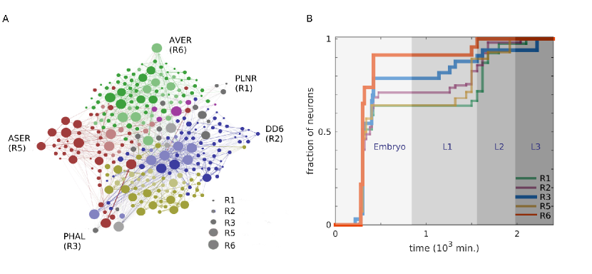
Figure 7: Neurons functioning as connectors between different network modules lead in development. (A) Schematic representation of the network of neurons belonging to the somatic nervous system of Caenorhabditis elegans, indicating the role of each neuron (indicated by the node size, see legend) in the mesoscopic structural organization of the network. This organization is manifest in the partitioning of the entire network into six structural modules Pan et al. (2010) which are characterized by relatively dense connections among neurons in each module compared to the connections between neurons belonging to different modules (node color representing the identity of a module to which a neuron belongs). Within each module, neurons can be further distinguished into those which have significantly higher number of connections to neurons within their own module (hubs) and those which do not (non-hubs). According to their intra- and inter-modular connectivity, every neuron is then classified into one of seven possible categories (see Methods), viz. R1: ultra-peripheral (non-hub nodes with all their connections confined to their own module), R2: peripheral (non-hub nodes with most of their connections occurring within their module), R3: satellite connectors (non-hub nodes having with many connections to other modules), R4: kin-less (non-hub nodes with connections distributed uniformly among all modules), R5: provincial hubs (hub nodes with a large majority of connections within their module), R6: connector hubs (hub nodes with many connections to other modules) and R7: global hubs (hub nodes with connections distributed uniformly among all modules). One representative neuron from each of the categories is separately indicated with a label identifying them by name (note that there are no neurons in the C. elegans somatic nervous system which belong to categories R4 or R7). Neurons which function as connectors, e.g., AVER (R6) and PHAL (R3), are seen to have links to neurons belonging to many different modules (as indicated by the node color of their network neighborings) while neurons belonging to other categories are connected predominantly to neurons within their own modules (indicated by their network neighborhood being almost homogeneous in terms of node color). Neighbors of labeled neurons are either shown clustered around them (for PLNR, DD6, PHAL and ASER) or indicated by a lighter shade of node color (for AVER). (B) Distribution of differentiation times of neurons belonging to the different network functional role categories indicate that the development of those functioning as connectors (viz., R3 and R6) lead the other classes of neurons in the embryonic, as well as, L1 stages. In particular, more than $90\%$ of connector hubs have appeared before hatching, while for the non-connector categories (R1, R2 and R5), $70\%$ or less of their members would have differentiated by that time.

Specifically, we focus on the six previously identified topological modules of the C. elegans neuronal network, which are groups of neurons that have markedly more connections with each other than to neurons belonging to other modules Pan et al. (2010). We classify all the neurons by identifying their function in terms of linking the elements belonging to a module, as well as, connecting different modules to each other Guimerà and Amaral (2005a). This is done by measuring (i) how significantly well connected a neuron is to other cells in its own module by using the within-module degree $z$-score, and (ii) how dispersed the connections of a neuron are among the different modules by using the participation coefficient $P$ Guimerà and Amaral (2005b). Cells are classified as hub or non-hub based on the value of $z$ (see Methods for details). The hubs can be further classified based on the value of $P$ as (R5) local or provincial hubs, that have most of their links confined within their own module and (R6) connector hubs, that have a substantial number of their connections distributed among other modules. The measured value of $P$ is also used to divide the non-hub neurons into (R1) ultra-peripheral nodes, which connect only to members of their own module, (R2) peripheral nodes, most of whose links are restricted within their module and (R3) satellite connectors, that link to a reasonably high number of neurons outside their module. Fig. 7 (A) shows the roles (indicated by node size) played by each neuron in the somatic nervous system of C. elegans using a schematic representation of the network. In principle, while it is also possible to have (R7) global hubs and (R4) kinless nodes, viz., hub and non-hub nodes that may connect to other neurons homogeneously, regardless of their module, none of the neurons appear to play such roles in the network.

Earlier investigation Pan et al. (2010) has already established that the connector hubs are crucial in coordinating most of the vital functions that the C. elegans nervous system has to perform. Indeed, $20$ of the $23$ neurons having this role are seen to occur in one or more functional circuits (discussed later). Their importance to the network is further reinforced by observing from Fig. 7 (B) that all but two of the neurons belonging to the R6 category appear early in the embryonic stage, and even the remaining ones, viz., AVFL/R (discussed earlier in the context of bilaterally symmetric neurons), differentiate by the end of L1 stage. By contrast, all other functional role categories have a much smaller fraction of their members appear in the early burst of development and have to wait till the L2 or L3 stage for the development of their full complement. In particular, we notice that the provincial hubs, despite having a relatively high degree, lag behind not only the connector hubs but also the satellite connectors (that have much lower degree) for most of the developmental period. This suggests that more than the degree, it is the distribution of the connections of a neuron among the different modules (quantified by the participation coefficient $P$), and thus its functional role in coordinating activity across different parts of the network, which is an important determinative factor for its appearance early in the developmental chronology of the nervous system.

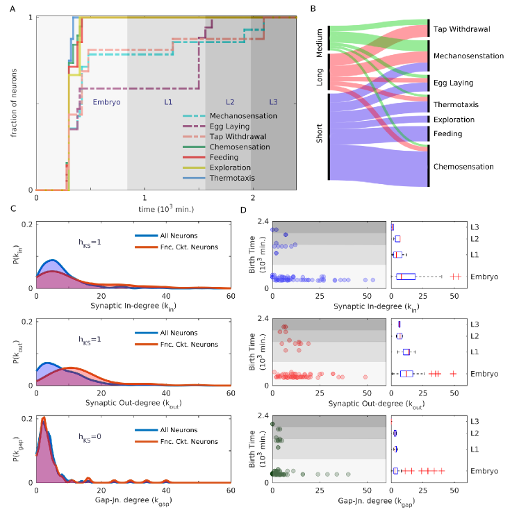
Figure 8: The developmental duration of functional circuit neurons are strongly indicative of their process length and connectivity. (A) Distribution of differentiation times of neurons that belong to any of seven previously identified functional circuits: (i) mechanosensation, (ii) egg laying, (iii) tap withdrawal, (iv) chemosensation, (v) feeding, (vi) exploration and (vii) thermotaxis. Note that the entire complement of neurons belonging to the functional circuits corresponding to (iv)-(vii) [shown using solid lines] have differentiated early in the embryo stage, while those for (i)-(iii) [shown using broken lines] are completed much later, viz., in the L2 and L3 stages. (B) The distribution of neurons having short, medium and long processes [indicated at left], among the different functional circuits [right]. We note a correlation between the morphological feature of neurite length and the development time of functional circuit neurons, viz., those in early developing circuits (iv-vii) predominantly have short processes, while those in later developing circuits (i-iii) mostly have medium to long processes. (C) Comparison between the distributions of the number of incoming and outgoing synaptic connections ($k_{in}$ [top panel] and $k_{out}$ [middle panel], respectively), as well as, gap junctions ($k_{gap}$ [bottom panel]) of neurons in the entire somatic nervous system (blue) and of the subset of functional circuit neurons (red). We note that the distribution of synaptic connections (both incoming and outgoing) for the functional circuit neurons is significantly different from that for the entire network, as indicated by the result of a two-sample Kolmogorov-Smirnov test at $5\%$ level of significance ($h_{KS}=1$), but not for gap junctions ($h_{KS}=0$). (D) Dispersion of $k_{in}$ (top panel), $k_{out}$ (middle) and $k_{gap}$ (bottom) for the functional circuit neurons differentiating at various times is shown in terms of the adjoining box plots where neurons are clustered into four groups according to the developmental stage during which they are born, viz., Embryo, L1, L2 or L3. In general, the distributions are far more broad for the early born neurons (Embryo) compared to those born later (L1-L3). Focusing on the functional circuit neurons that develop in the embryonic stage, we note that the distribution of incoming connections is more skewed than that for outgoing connections. The distribution of gap junctions is even more skewed, with outliers lying very far from the median.

Membership in functional circuits. In order to delve deeper into a possible association between the function(s) that a neuron performs in the mature nervous system and its developmental characteristics, specifically its place in the temporal sequence of appearance of the neurons, we now focus on several previously identified functional circuits of C. elegans. These are groups of neurons which have been identified by behavioral assay of individuals in which the cells have been removed (e.g., by laser ablation). As their absence results in abnormal or impaired performance of specific functions, these neurons are believed to be crucial for executing those functions, viz., (F1) mechanosensation Chalfie et al. (1985); Wicks and Rankin (1995); Sawin (1996), (F2) egg laying Waggoner et al. (1998); Bany et al. (2003), (F3) thermotaxis Mori and Ohshima (1995), (F4) chemosensation Troemel et al. (1997), (F5) feeding White et al. (1986); Chalfie et al. (1985); Gray et al. (2005), (F6) exploration White et al. (1986); Chalfie et al. (1985); Gray et al. (2005) and (F7) tap withdrawal Wicks and Rankin (1995, 1996). Note that several neurons belong to multiple functional circuits. Fig. 8 (A) shows that one can classify these seven functional circuits into two groups based on whether or not all the constituent neurons of a circuit appear during the early burst of development in the embryonic stage. Thus, while circuits for F3-F6 (shown using solid lines in the figure) have their entire complement of cells differentiate prior to hatching, circuits for F1, F2 and F7 lag behind (broken lines), with less than $60\%$ of the egg laying circuit having appeared at the time of hatching. Indeed, for the entire set of neurons for the latter circuits to emerge one has to wait until the much later L2 (for F2) or L3 (for F1 and F7) stages [note that out of the 16 neurons in the F7 circuit, 15 are common to those belonging in the F1 circuit, making the former almost a subset of the latter]. The temporal order in which the circuits appear makes intuitive sense in that, the functions that are vital for survival of the organism at the earliest stages (such as thermotaxis or chemosensation) have all the components of their corresponding circuits completed much earlier than those functions such as egg laying which are required only in the adult worm.

An intriguing relation between process lengths of neurons and their occurrence in different functional circuits is suggested by Fig. 8 (B), from which we see that circuits which have their entire complement of neurons differentiate early, viz., F3-F6, are dominated by neurons having short processes. In contrast, circuits such as F1, F2 and F7 that take much longer to have all their members appear comprise a large number of neurons with medium or long processes. This association between a morphological feature (viz., neurite length) of a functionally important neuron and its time of appearance suggests a possible connection with the process length homophily, viz., preferential connection between neurons having short processes, mentioned earlier. Neurons with short processes that belong to the “early” functional circuits are mostly chemosensory or interneurons that are all located in the head region. To perform their task these neurons only need to connect to each other, whose cell bodies are mostly in close physical proximity of each other. Moreover, having their synapses localized within a small region allows them to be activated by neuromodulation through diffusion of peptides and other molecules Bargmann (2012); Bentley et al. (2016). This assumes significance in light of our observation that process length homophily between short process neurons is marginally enhanced in the head. The value of $Q$, a quantitative measure of homophily introduced earlier, is 0.11 (for synapse, for gap junctions it is $0.12$) for early born short process neurons which have their cell bodies located in the head region. In contrast, when we consider all short process neurons, $Q$ is $0.067$ for synapse and $0.073$ for gap junction, respectively. Thus, the process length homophily we reported earlier could arise in short process neurons because of functional reasons.

We shall now see how consideration of functional circuits help in obtaining a deeper understanding of the nuanced relation between the degree of a neuron and the time of its birth that was discussed above (in the context of mesoscopic functional roles of neurons). As seen in Fig. 8 (C), neurons belonging to the functional circuits show a significantly different distribution for the number of synaptic connections (both incoming and outgoing) from that of the entire system, as indicated by the results of two-sample Kolmogorov-Smirnov test (test statistic $h_{KS}=1$) at $5\%$ level of significance. Thus, the set of functionally critical neurons - which, on average, have a larger number of connections than a typical neuron in the somatic nervous system - may need to be treated separately from the other neurons when we examine how synaptic degree correlates with birth time. In contrast, their gap junctional degree distributions cannot be distinguished from that of all neurons, as indicated by the result ($h_{KS}=0$) for the statistical test of significance.

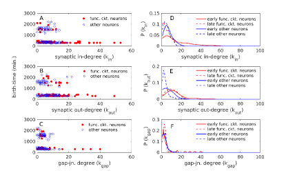
Figure S12: The number of synaptic connections of a neuron is influenced by its functional criticality, as well as, the developmental epoch in which it appeared. (A-C) Scatter plots indicating the relation between the time of appearance of a neuron and its number of (A) incoming synaptic connections from other cells (synaptic in-degree), (B) outgoing synaptic connections to other cells (synaptic out-degree) and (C) gap junctions with other cells (gap-junctional degree). Filled circles represent neurons belonging to any of seven previously identified functional circuits (see Fig. 8 in main text) while unfilled circles show other neurons. (D-F) Probability distributions of different types of connections for neurons categorized in terms of those which are functionally critical, i.e., belong to a functional circuit (red), or not (blue), and whether they appear in the early (solid curve) or late (broken curve) developmental epochs. The different panels correspond to (D) synaptic in-degree, (E) synaptic out-degree and (F) gap-junctional degree. Synaptic in-degree for functionally critical, early-born neurons is seen to have a heavy-tailed distribution which is significantly different from that of the other types of neurons (in terms of a $2$-sample Kolmogorov-Smirnov test at $5\%$ level of significance). The heavy tail arises from the appearance of a set of neurons having exceptionally high in-degree [the filled circles having $k_{in}>20$ shown in panel (A)], that play the role of connector hubs in the nervous system. These correspond to the early born R6 category neurons [see Fig. 7 (B)]. On excluding these, the synaptic in-degree distributions of the early-born functional circuit neurons become indistinguishable from that of other categories of neurons. For the case of synaptic out-degree, however, the distributions for functionally critical neurons that are born at different epochs are statistically indistinguishable. However, for other neurons, the distribution of those that are born in the later, post-embryonic developmental burst are distinct from those that are born early (demonstrated by a $2$-sample Kolmogorov-Smirnov test at $5\%$ level of significance). This statistically significant difference between the outgoing connections of early and late-born neurons could arise from the former neurons being present for a much longer period during which they can send out synapses. Distributions of gap junctional connections for all categories of neuron appear to be statistically indistinguishable, suggesting that gap junction formation is relatively unaffected by the functional criticality or time of appearance of the neurons.

Considering only the neurons that appear in functional circuits, we observe that most of the neurons having a large number of synaptic connections (particularly, incoming ones) do tend to appear early [Fig. 8 (D)]. On comparing the distributions of synaptic in-degree separately for early and late appearing functionally critical neurons (see Supplementary Material, Fig. S12) we note that their difference is indeed statistically significant. However, a deeper scrutiny shows that the significant deviation between the two is a result of the occurrence of the $14$ largest in-degree neurons in the group that is born early, all of which turn out to be connector hubs (described earlier). On removing these, the in-degree distributions for early and late born neurons belonging to the functional circuits become indistinguishable. Thus, the distinction between the two sets of neurons in terms of their degree can be traced to the distinct functional roles, rather than simply their order of appearance in the developmental chronology. Moreover, when we consider the rest of the neurons of the somatic nervous system, the early and late born ones cannot be distinguished in terms of their in-degree distributions. Thus, birth time does not appear to be a significant determinant for the connections that are received by a post-synaptic neuron.

When we consider the distribution of the synaptic out-degree we see a very different result. The distributions for the early and late born functionally critical neurons turn out to be statistically indistinguishable (despite the appearance of a few extreme outliers such as the command interneurons AVAL/R and PVCL/R). In contrast, the rest of the neurons show a much broader distribution (statistically distinguishable using a two-sample Kolmogorov-Smirnov test) for the neurons that are born early, compared to those which are born late. This is consistent with the assumption that pre-synaptic neurons that exist for a longer period during development, are able to form many more connections than those neurons which appear later (the latter presumably having less time to form connections before the maturation of the nervous system). From this perspective, it is thus striking that the late born functionally critical neurons have as many connections as they do (making them statistically indistinguishable from the early born set), and is possibly related to their inclusion in the functional circuits.

When we consider the gap-junctional degree distributions, we observe that there is no statistically significant difference between the distributions for early and late born neurons, whether they be functionally critical or other neurons. The box plots showing the nature of the distribution at different developmental stages are all fairly narrow [bottom panel of Fig. 8 (D)], even though the embryonic one shows several outliers with the four farthest ones being the command interneurons AVAL/R and AVBL/R that appear in four functional circuits, viz., those of mechanosensation, tap withdrawal, chemosensation and thermotaxis. These, in fact, correspond to the outlying peaks of the $k_{gap}$ distribution, located on the extended tail at the right of the bulk [bottom panel of Fig. 8 (C)]. Indeed, the outliers in each of the distributions (for $k_{in}$, $k_{out}$ and $k_{gap}$), that appear only at the embryonic stage, almost always happen to be command interneurons. Of these, AVAL/R are common across the distributions and the fact that they occur in four of the known functional circuits underlines the relation between function, connectivity and the temporal order of appearance of neurons that we have sought to establish in this paper.

III Discussion

The nervous system, characterized by highly organized patterns of interactions between neurons and associated cells, is possibly the most complex of all organ systems that is assembled in an animal embryo over the course of development Wolpert and Tickle (2011). For this neural network to be functional, it is vital that the cells are able to form precisely delineated connections with other cells that will give rise to specific actions. This raises the question of how the “brain wiring problem” is resolved during the development process of an organism. In addition to the processes of cellular differentiation, morphogenesis and migration that are also seen in other tissue, cells in the nervous system are also capable of activity which modulates the development of the neighboring cells they may interact with. Processes extending from the neuronal cell bodies are guided towards designated targets by molecular cues, and the resulting connections are subsequently refined (e.g., by pruning) through the activity of the cells themselves. In this paper we have looked at a more abstract “algorithmic” level of guiding principles that can help in connecting the details of cellular wiring at the implementation level of molecular mechanisms with the final result, viz., the spatial organization and connection topology of an entire nervous system. Using the relatively simple nervous system of the model organism Caenorhabditis elegans, whose entire developmental lineage and connectivity are completely mapped, we have strived to show how development itself provides constraints for the design of the nervous system.

One of our key findings is that neurons with similar attributes, specifically, (i) the lengths of the processes extending from the cell body (short/ medium/ long), (ii) the birth cohort to which they belong (early/ late), (iii) the extent of shared lineage and (iv) bilateral symmetry pairing (left/ right), exhibit a significant preference for connecting to each other (homophily). Moreover, excepting for homophily on the basis of lineage relations (which is seen for synaptic connections only), all other types of homophily are manifested by both the connection topology of the network of chemical synapses, as well as, that of electrical gap-junctions, despite the fundamental differences in the nature of these distinct types of links.

We have already discussed earlier a plausible mechanism by which homophily based on lineage would be observed only in the case of synapses. This is based on the hypothesis that synaptogenesis occurs much earlier than the formation of gap junctions during development. As neurons are displaced from their initial locations while retaining the synaptic connections that have formed already, cells that share common lineage tend to move apart. Thus, when gap-junctions form much later between adjacent cells, the connected neurons may have quite different lineages - disrupting any relation between lineage distance and probability of connection via gap-junction. An alternative possibility that may also explain the specificity of lineage homophily to synapses is related to the suggestion that synaptogenesis could be guided by cellular labels that are specified by a combinatorial code of neural cell adhesion proteins Emmons (2016). In this scenario, cells that are close in terms of their lineage will be likely to share several of the recognition molecules that will together determine the label code. Thus, if a sufficiently large number of these determinants match each other, it could promote synapse formation between such cells, resulting in lineage homophily. We would also like to note that, apart from playing an important role in determining the topological structure of the synaptic network, lineage relations between neurons also appear to shape the spatial organization of neurons by segregating them into different ganglia.

In addition to investigating the probability that a connection will occur between a pair of neurons during development, our study also considers how the distance between cell bodies of the neurons thus connected is distributed. Our results suggest that for synapses, the process length of the pre-synaptic neuron is a decisive factor in determining the separation that is allowed between the neuronal partners. Birth time also appears to play a role, particularly, in the case of long-range connections, i.e., between neurons whose cell bodies are separated by more than two-thirds of the worm body length. Specifically, such connections occur between pre-synaptic neurons that are born early and post-synaptic neurons that are born late, much more often than is expected by chance. This suggests the existence of an active process for the formation of such long-range connections, for example, using fasciculation as an axon guidance mechanism White et al. (1986); Kaiser (2017). The latter involves a few pioneer neurons with long process lengths acting as supporting pathways that guide axons of the later developing neurons. This may also underlie a triadic closure-like phenomenon in the network Newman (2010); Easley and Kleinberg (2010) (viz., two neurons having links to one or more common neighbors that have an increased likelihood of being connected to each other). Such a process is known to yield strongly clustered networks with high communication efficiency Davidsen et al. (2002); Brot et al. (2015) and could be responsible for the appearance of the so-called “common neighbor rule” that has been reported in the C. elegans connectome Azulay et al. (2016).

Our results also indicate that the temporal sequence in which neurons appear during development of the nervous system is linked to their functional identities. The simplest of these identities is simply the basic functional type of a neuron, viz., whether it is sensory, motor or interneuron. The neurons belonging to these different types not only differ in terms of the cells they connect to (for instance, only motor neurons connect to muscles and sensory neurons are the only ones to receive connections from receptors, while interneurons connect to all types of neurons) but also in their molecular inventory. While their lineage does not show any significant differences, the different functional types of neurons do appear to segregate to a certain extent in terms of their time of appearance. Specifically, we find that the bulk of neurons that are born in the late, post-embryonic burst of development are motor neurons. Our results suggest that there may be temporal cues that appear late in the process of development which are responsible for the specialization of neurons into different functional types according to their time of birth.

At a higher, mesoscopic level of organization of the network structure, we have considered the functional role of neurons in coordinating the activity of different topological modules of the network. We show that this allows us to obtain a much more nuanced picture of how the number of connections that a neuron has with other neurons, affects its place in the temporal sequence in which neurons appear during development. Thus, rather than a simple case of just the degree (the total number of connections) of a neuron deciding its precedence in the sequence, it is actually the connector neurons (connector hubs, as well as, satellite connectors) which are the earliest to appear. We also examine in detail the subset of neurons that have been identified as belonging to one or more functional circuits in the C. elegans. We observe that membership of a specific functional circuit does determine the order in which these neurons appear, with certain circuits, such as those responsible for chemosensation, emerging early (before hatching) while others circuits, such as those for mechanosensation and egg-laying, appear much later (after hatching). In turn, the time of appearance of functional circuits determines to an extent the morphological properties, such as the process lengths, of their constituent neurons.

The observations reported in this paper are an attempt at resolving the “wiring problem” for the C. elegans nervous system by focusing at a level that is intermediate between the molecular mechanism-level details of developmental processes and the resulting structural organization of the entire somatic nervous system. Specifically, we have attempted to uncover general “algorithmic” principles governing the design of the neuronal network, which will allow linking the complicated molecular machinery involved to the equally complicated spatial and topological description of the nervous system. The next step in this approach will involve delineating exactly how these governing principles (such as the various types of homophily) are implemented by molecular mechanisms, and how genetics may be relating the temporal sequence of appearance of neurons to their functional identities. Experimental and theoretical progress towards this direction would enable us to achieve a seamless understanding of nervous system development involving different scales.

IV Materials and Methods

IV.1 Data

Connectivity and lineage. We have used information about the network connectivity and lineage distance between $279$ connected neurons of the C. elegans somatic nervous system from the database published in Ref. Varshney et al. (2011), accessible from an online resource for behavioral and structural anatomy of the worm WormAtlas et al. (2019). This is an updated and revised version of connectivity data obtained through serial section electron micrography that first appeared in Ref. White et al. (1986).

Time of birth for neurons. We have transcribed the time of appearance of each neuron over the course of development of the organism from lineage charts provided in Refs. Sulston and Horvitz (1977); Sulston et al. (1983). This is provided in Table LABEL:T4 in the Supplementary Material.

Time of cell-division for progenitor cells The information about the time of each cell-division, starting from the zygote, that occurs over the course of development of the C. elegans somatic nervous system, and which has been used for generating the chrono-dendrograms shown here, are provided in Refs. Sulston and Horvitz (1977); Sulston et al. (1983), accessible from an online interactive visualization application Bhatla (2011).

Physical distance. We have used information on the positions of the neurons from the database reported in Ref. Choe et al. (2004), accessible online from https://www.dynamic-connectome.org/. The location information provides coordinates of each neuronal cell body projected on a two-dimensional plane defined by the anterior-posterior axis and the dorsal-ventral axis.

Neuronal process length. Lengths of the processes extending from each cell body has been estimated from the diagrams of the neurons provided in Appendix 2, Part A of Ref. Wood (1988) and from an online resource for the anatomy of the worm WormAtlas et al. (2019).

Ganglia and functional types. The information about the ganglion to which a neuron belongs and the functional type of each neuron (viz., sensory, motor or interneuron) has been obtained from the database provided in Ref. Achacoso and Yamamoto (1991).

Functional circuits. The identities of the neurons belonging to each of the functional circuits referred to here is available from the Supporting Information (Table S2) of Ref. Pan et al. (2010).

IV.2 Modularity

A network can be partitioned into several communities or topological modules, defined such that neurons in a given module have a much higher probability of being connected to other neurons in the module compared to neurons that do not belong to it, by maximizing the modularity value $Q$ Newman, Mark E.J. (2004) associated with a given partitioning, viz.,

$$Q=\frac{1}{L}\sum_{i,j}\Big{[}A_{ij}-\frac{k_{i}^{in}k_{j}^{out}}{L}\Big{]}\delta_{c_{i}c_{j}}.$$ (1)

Here, A is the adjacency matrix describing the connections of the network ($A_{ij}=1$, if neuron $i$ receives a connection from neuron $j$, and $=0$ otherwise). The in-degree and out-degree of a node $i$ are given by $k_{i}^{in}=\sum_{j}A_{ij}$ and $k_{j}^{out}=\sum_{i}A_{ij}$, respectively. The total number of links in the network is given by $L=\sum_{i,j}A_{ij}$. The Kronecker delta function $\delta_{ij}=1$, if $i=j$, and $0$, otherwise. The indices $c_{i},c_{j}$ refer to the modules to which the neurons $i$ and $j$, respectively, belong. For an undirected network, such as that defined by the set of connections between neurons via gap-junctions, the adjacency matrix is symmetric (i.e., $A_{ij}=A_{ji}$) and $k_{i}^{in}=k_{i}^{out}=k_{i}$. The value of $Q$ expresses the bias that a neuron has to connect to members of its own community (which could be defined in terms of any distinguishing characteristic of the cells, e.g., process length), relative to the null model. The latter corresponds to an unbiased, homogeneous network where the probability of connection between two nodes is proportional to the product of their respective degrees.

IV.3 Bimodality coefficient

The bimodal nature of a probability distribution can be characterized by calculating its bimodality coefficient Pfister et al. (2013):

$$BC=\frac{m^{2}_{3}+1}{m_{4}+3\cdot\frac{(n-1)^{2}}{(n-2)(n-3)}},$$ (2)

where $m_{3}$ is the skewness, $m_{4}$ is the excess kurtosis and $n$ represents the sample size. A distribution is considered to be bimodal if $BC>BC^{*}$ where $BC^{*}=5/9$. This benchmark value corresponds to a uniform distribution, and if $BC<BC^{*}$, the distribution is considered unimodal.

IV.4 Process length randomization.

To establish statistically significant evidence for process length homophily, the empirical network is compared with an ensemble of networks obtained from the empirical one by randomly assigning process lengths (short, medium and long) to the neurons while ensuring that the total number of neurons in each process length category, viz., $N_{S}$, $N_{M}$ and $N_{L}$, respectively, (as well as, all other properties of the network, such as connectivity) remains unchanged. In practise, this is done by first partitioning the neurons into three communities according to process length and ordering the neurons in sequence according to the module they belong. Thus, neurons $i=1,\ldots,N_{S}$ have short processes, neurons $i=N_{S}+1,\ldots,N_{S}+N_{M}$ have medium length processes, and neurons $i=N_{S}+N_{M}+1,\ldots N_{S}+N_{M}+N_{L}$ have long processes. Then, to create each member of the surrogate ensemble, this sequence is randomly permuted and the first $N_{S}$ neurons are assigned short process length, the next $N_{M}$ neurons are assigned medium process length and the remaining $N_{L}$ neurons are assigned long process length. The modularity $Q$ calculated for networks with such randomized module membership (corresponding to a null model where process length homophily is non-existent by design) is expected to be small.

IV.5 Network randomization constrained by neuronal process lengths

An ensemble of surrogate networks is constructed by randomizing the connections of the empirical network, subject to different constraints. Each member of the ensemble is constructed by repeatedly selecting a pair of directed connections, e.g., $p\rightarrow q$ and $u\rightarrow v$, and rewiring them such that the in-degree and out-degree of each neuron remains invariant, i.e., $p\rightarrow v$ and $u\rightarrow q$. If these new connections already exist, this rewiring is disallowed and a new random selection for a pair of directed connections done. In addition, information about the spatial location of the cell bodies and that of the process lengths of neurons are used to further constrain the connections. This ensures that un-physical connections, such as between two short process neurons (i.e., each has a process length that is less than a third of the body length of the nematode) whose cell bodies are placed apart by more than $2L/3$ ($L$: total body length of the worm), do not appear through the randomization. In practise, this constraint is imposed as follows. In absence of precise knowledge of the length of each process, depending on the length process category to which each neuron belongs, an uniformly distributed value (lying between $[0,L/3]$ for short, between $[L/3,2L/3]$ for medium and $[2L/3,L]$ for long process neurons) is assigned as the process length for a neuron. The distance between the cell bodies of a pair of neurons that have been selected randomly for connection is then compared against the sum of their process lengths. If the latter is greater than the former, the connection is allowed, else not. The rewiring steps are repeated $5\times 10^{5}$ times to construct each of the randomized networks belonging to the surrogate ensemble. The entire ensemble consists of $100$ realizations of such randomized networks.

IV.6 Lineage randomization

To establish that neurons belonging to the same ganglion are closely related in terms of their lineage, we compare the properties of the lineage distance distribution within and between ganglia obtained for the empirical network with those obtained upon randomizing the lineage relations. This is done by repeatedly selecting a pair of neurons at random on the lineage tree and exchanging their positions on the tree. This procedure is carried out $10^{4}$ times for a single realization. This ensures that, in the randomized networks, the lineage relation between neurons is completely independent of whether they belong to the same ganglion or not. In order to compare the properties of the empirical network with its randomized version, an ensemble of $10^{3}$ realizations is considered. To quantify the deviation of the empirical intra- and inter-ganglionic lineage distance distributions from their randomized counterparts, we measure the $z$-score of the corresponding means and coefficients of variation (CV). The $z$-score is a measure for the extent of deviation of an empirical property $x_{emp}$ from the mean of the randomized counterparts, $\langle x_{rand}\rangle$, scaled by the standard deviation of the randomized counterparts, viz.,

$$z=\frac{x_{emp}-\langle x_{rand}\rangle}{\sqrt{\langle x_{rand}^{2}\rangle-\langle x_{rand}\rangle^{2}}}.$$ (3)

IV.7 Surrogate ensemble for comparison with average cell body distance between connected neuronal pairs

To see whether the distance $d$ between cell bodies of connected pairs of neurons [where the members of the pair could belong to either the same or different process length categories, viz., short (S), medium (M) and long (L)] is distributed in a significantly different manner from that between all pairs of neurons, we have constructed surrogate ensembles. For each realization belonging to such an ensemble, a number of cell body distances is sampled from the set of all distances $D$ between each neuronal pair, such that the sample size is same as the number of connected neural pairs. The entire ensemble consists of $10^{3}$ such sampled sets. To see whether the observed difference between $\langle d_{XY}\rangle$ and $\langle D\rangle_{X,Y}$, where $X,Y\in\{S,M,L\}$, can be explained simply as finite size fluctuation, we have evaluated the corresponding $z$-scores, viz.,

$$z_{XY}=\frac{d^{emp}_{XY}-\langle d^{rand}_{XY}\rangle}{\sqrt{\langle(d^{rand}_{XY})^{2}\rangle-\langle d^{rand}_{XY}\rangle^{2}}}.$$ (4)

IV.8 Lineage tree rung determination

The order of the rung in the lineage tree that a cell belongs to is obtained from the lineage information of the cell (available from Ref. WormAtlas et al. (2019)). This indicates the series of cell divisions, starting from AB (which results from the division of the single cell zygote) that leads to a particular neuron, e.g., ABprpapaap. The letters a (anterior), p (posterior), l (left) and r (right) which follow AB, indicate the identity of the progenitor cells that result from subsequent cell divisions eventually terminating in a differentiated neuron. As the rung that a neuron belongs to is given by the number of cell divisions (starting from the zygote) that leads to the differentiated cell, we simply count the total number of letters (AB is counted as a single letter) specifying the lineage of a cell to determines its rung.

IV.9 Stochastic branching model for lineage tree

To theoretically describe the generative process leading to the observed lineage tree for the cells belonging to the C. elegans somatic nervous system, we have used a stochastic asymmetric branching model. Starting from the single cell zygote, each cell division leads to at most two daughter cells, with independent probabilities $P1$ and $P2$ ($P1\geq P2$) for the occurrence of each of the two branches. Thus, based on the probabilities $P1$ and $P2$, at each step of the generative process any one of the following three events can happen: (i) proliferation occurs along both branches, (ii) only one branch appears (the other branch leading to either apoptosis or a non-neural cell fate), and, (iii) there is no branching so that a terminal node of the tree is obtained (i.e., the cell differentiates into a neuron). Estimation of $P1$ and $P2$ from the empirical lineage tree suggests that proliferation markedly reduces after rung 10. Incorporating this in the model by decreasing the probabilities $P1,P2$ after rung $10$ results in successive reduction of the branching, eventually coming to a stop. The ensemble of $10^{3}$ simulated lineage trees produced by the process matches fairly well with the empirical lineage tree in terms of the number of terminal nodes, the distribution of the rungs occupied by each cell and the distribution of lineage distances between the differentiated neurons (see Supplementary Material, Fig. S4).

IV.10 Classifying neurons according to their role in the mesoscopic structural organization of the network

The functional importance of a neuron vis-a-vis its own topological module (defined above in Sec. IV.2), as well as, the entire nervous system, can be quantified in terms of its intra- and inter-modular connectivity Pan et al. (2010). For this purpose we use the two metrics Guimerà and Amaral (2005a): (i) the within module degree $z$-score ($z$) and (ii) the participation coefficient ($P$).

In order to identify neurons that have a significantly large number of connections to the other neurons belonging to their module, we calculate the within module degree $z$-score defined as

$$z_{i}=\frac{\kappa^{i}_{c_{i}}-\langle\kappa^{j}_{c_{i}}\rangle_{j\in c_{i}}}{\sqrt{\langle(\kappa^{j}_{c_{i}})^{2}\rangle_{j\in c_{i}}-\langle\kappa^{j}_{c_{i}}\rangle^{2}_{j\in c_{i}}}},$$ (5)

where $\kappa^{i}_{c}$ is the number of connections that a neuron $i$ has to other neurons in its community (labeled $c$) and the average $\langle\ldots\rangle_{j\in c}$ is taken over all nodes in the community. Following Ref. Pan et al. (2010), we identify neurons having $z\geq 0.7$ as hubs, while the remaining are designated as non-hubs.

The neurons are also distinguished in terms of how many well connected they are to neurons belonging to other communities. For this purpose we measure the participation coefficient $P$ of a neuron, which is defined as

$$P_{i}=1-\sum^{m}_{c=1}(\frac{\kappa^{i}_{c}}{k_{i}})^{2},$$ (6)

where $\kappa^{i}_{c}$, as above, is the number of connections that the neuron has to other neurons in its own module (labeled $c$) and $k_{i}=\sum_{c}\kappa^{i}_{c}$ is the total degree of node $i$. Neurons that have their connections homogeneously distributed among all modules will have a $P$ close to $1$, while $P=0$ if all of their connections are confined within their module. Based on the value of $P$, following Ref. Pan et al. (2010) we have classified the non-hub neurons as ultra-peripheral (R1: $P\leq 0.05$), peripheral (R2: $0.05<P\leq 0.62$), satellite connectors (R3: $0.62<P\leq 0.8$) and kin-less nodes (R4: $P>0.8$), while hub neurons are segregated into provincial hubs (R5: $P\leq 0.3$), connector hubs (R6: $0.3<P\leq 0.75$) and global hubs (R7: $P>0.75$).

IV.11 Statistics

Two-sample Kolmogorov-Smirnov (KS) test Massey (1951) has been used to compare between pairs of samples (e.g., the degrees of neurons belonging to different categories) to determine whether both of them are drawn from the same continuous distribution (null hypothesis) or if they belong to different distributions. For this purpose we have used the kstest2 function in MATLAB Release 2010b, with the value of the parameter $\alpha$ which determines threshold significance level set to $0.05$.

Kernel smoothened density function Bowman and Azzalini (1997) has been used to estimate the probability distribution functions of different quantities (e.g., distances between cell bodies of neurons). For this purpose we have used the ksdensity function in MATLAB Release 2010b with a Gaussian kernel.

Author Contributions

AP, NC and SS conceived the study and designed the methodology, AP collected the data, performed the investigation and did the visualization, AP, NC and SS analyzed the results and wrote the paper, SS supervised the study.

Conflict of interest

The authors declare that they have no conflict of interest.

Table S1: Process length homophily among neurons segregated into groups comprising cells with long, medium and short processes, respectively. The extent of homophily is quantified by the modularity measure $Q$ computed over the different classes of neurons (which are considered to be the communities or modules for the purpose of calculation of $Q$). The empirical values are compared with that calculated from the corresponding surrogate ensemble obtained by randomly shuffling the process length categories of the empirical network keeping the network connections invariant. Note that the $Q$ values are significantly higher than that expected by chance (as seen for the surrogate ensemble) for the entire network, as well as, individually for almost all process length categories, suggesting process length homophily in both synaptic and gap-junction connections between neurons.

	Synapse		Gap-junction
Process length	Q (empirical)	Q (randomized)	Q (empirical)	Q (randomized)
Long	0.044	-0.000 $\pm$ 0.006	0.051	-0.001 $\pm$ 0.008
Medium	0.006	-0.001 $\pm$ 0.004	0.01	-0.001 $\pm$ 0.008
Short	0.067	-0.001 $\pm$ 0.003	0.073	-0.002 $\pm$ 0.011
All	0.117	-0.002 $\pm$ 0.010	0.134	-0.004 $\pm$ 0.020

Table S2: For synaptically connected neurons, process length of the pre-synaptic neuron primarily decides the average distance between the cell bodies. Statistically significant deviation (measured in terms of $z$-score) between the average distance $\langle d\rangle$ of cell bodies in pairs of connected neurons (having short, medium or long processes) and the average distance $\langle D\rangle$ between any pair of neurons randomly sampled from the same process length categories. The latter average is calculated over a set having the same number of pairs as for the set of connected pairs. Note that except for two cases (pre-synaptic long process to post-synaptic short process and pre-synaptic medium process to post-synaptic long process, shown in bold font), connections between cells in all other process length categories tend to be much shorter than that expected by chance, as indicated by $z<0$.

Synapse
	Pre-synaptic
Post-synaptic	Short	Medium	Long
Short	-12.07	-1.79	1.79
Medium	-9.13	-3.52	-0.29
Long	-7.15	0.9	-1.19
Gap-junction
	Short	Medium	Long
Short	-6.47	-6.22	-4.01
Medium	-6.22	-5.16	-4.47
Long	-4.01	-4.47	-2.16

Table S3: Neurons belonging to the somatic nervous system of C. elegans segregated into those which are born in the early (embryonic) and those born in the late (post-embryonic) developmental bursts. The respective lineage information and functional description are also provided. Motor neurons are indicated in red. We note that motor neurons that appear early mostly innervate dorsal muscles, whereas, motor neurons that appear late primarily innervate ventral muscles. All information shown here is obtained from WormAtlas WormAtlas et al. (2019).

Early Born Neurons
Neurons	Lineage	Description
ADAL	AB plapaaaapp	Ring interneuron
ADAR	AB prapaaaapp	Ring interneuron
ADEL	AB plapaaaapa	Anterior deirid, sensory neuron
ADER	AB prapaaaapa	Anterior deirid, sensory neuron
ADFL	AB alpppppaa	Amphid neuron
ADFR	AB praaappaa	Amphid neuron
ADLL	AB alppppaad	Amphid neuron
ADLR	AB praaapaad	Amphid neuron
AFDL	AB alpppapav	Amphid finger cell
AFDR	AB praaaapav	Amphid finger cell
AIAL	AB plppaappa	Amphid interneuron
AIAR	AB prppaappa	Amphid interneuron
AIBL	AB plaapappa	Amphid interneuron
AIBR	AB praapappa	Amphid interneuron
AIML	AB plpaapppa	Ring interneuron
AIMR	AB prpaapppa	Ring interneuron
AINL	AB alaaaalal	Ring interneuron
AINR	AB alaapaaar	Ring interneuron
AIYL	AB plpapaaap	Amphid interneuron
AIYR	AB prpapaaap	Amphid interneuron
AIZL	AB plapaaapav	Amphid interneuron
AIZR	AB prapaaapav	Amphid interneuron
ALA	AB alapppaaa	Neuron, sends processes laterally and along dorsal cord
ALML	AB arppaappa	Anterior lateral microtubule cell
ALMR	AB arpppappa	Anterior lateral microtubule cell
ALNL	AB plapappppap	Neuron associated with ALM
ALNR	AB prapappppap	Neuron associated with ALM
ASEL	AB alppppppaa	Amphid neurons, single ciliated endings
ASER	AB praaapppaa	Amphid neurons, single ciliated endings
ASGL	AB plaapapap	Amphid neurons, single ciliated endings
ASGR	AB praapapap	Amphid neurons, single ciliated endings
ASHL	AB plpaappaa	Amphid neurons, single ciliated endings
ASHR	AB prpaappaa	Amphid neurons, single ciliated endings
ASIL	AB plaapapppa	Amphid neurons, single ciliated endings
ASIR	AB praapapppa	Amphid neurons, single ciliated endings
ASJL	AB alpppppppa	Amphid neurons, single ciliated endings
ASJR	AB praaappppa	Amphid neurons, single ciliated endings
ASKL	AB alpppapppa	Amphid neurons, single ciliated endings
ASKR	AB praaaapppa	Amphid neurons, single ciliated endings
AUAL	AB alpppppppp	Neuron, process runs with amphid processes but lacks ciliated ending
AUAR	AB praaappppp	Neuron, process runs with amphid processes but lacks ciliated ending
AVAL	AB alppaaapa	Ventral cord interneuron
AVAR	AB alaappapa	Ventral cord interneuron
AVBL	AB plpaapaap	Ventral cord interneuron
AVBR	AB prpaapaap	Ventral cord interneuron
AVDL	AB alaaapalr	Ventral cord interneuron
AVDR	AB alaaapprl	Ventral cord interneuron
AVEL	AB alpppaaaa	Ventral cord interneuron, like AVD but outputs restricted to anterior cord
AVER	AB praaaaaaa	Ventral cord interneuron, like AVD but outputs restricted to anterior cord
AVG	AB prpapppap	Ventral cord interneuron
AVHL	AB alapaaaaa	Neuron, mainly postsynaptic in ventral cord and presynaptic in the ring
AVHR	AB alappapaa	Neuron, mainly postsynaptic in ventral cord and presynaptic in the ring
AVJL	AB alapapppa	Neuron, synapses like AVHL/R
AVJR	AB alapppppa	Neuron, synapses like AVHL/R
AVKL	AB plpapapap	Ring and ventral cord interneuron
AVKR	AB prpapapap	Ring and ventral cord interneuron
AVL	AB prpappaap	Ring and ventral cord interneuron and an excitatory GABAergic motor neuron for rectal muscles. Few synapses
AWAL	AB plaapapaa	Amphid wing cells, neurons having ciliated sheet-like sensory endings closely associated with amphid sheath
AWAR	AB praapapaa	Amphid wing cells, neurons having ciliated sheet-like sensory endings closely associated with amphid sheath
AWBL	AB alpppppap	Amphid wing cells, neurons having ciliated sheet-like sensory endings closely associated with amphid sheath
AWBR	AB praaappap	Amphid wing cells, neurons having ciliated sheet-like sensory endings closely associated with amphid sheath
AWCL	AB plpaaaaap	Amphid wing cells, neurons having ciliated sheet-like sensory endings closely associated with amphid sheath
AWCR	AB prpaaaaap	Amphid wing cells, neurons having ciliated sheet-like sensory endings closely associated with amphid sheath
BAGL	AB alppappap	Neuron, ciliated ending in head, no supporting cells, associated with ILso
BAGR	AB arappppap	Neuron, ciliated ending in head, no supporting cells, associated with ILso
BDUL	AB arppaappp	Neuron, process runs along excretory canal and into ring, unique darkly staining synaptic vesicles
BDUR	AB arpppappp	Neuron, process runs along excretory canal and into ring, unique darkly staining synaptic vesicles
CEPDL	AB plaaaaappa	Cephalic neurons, contain dopamine
CEPDR	AB arpapaappa	Cephalic neurons, contain dopamine
CEPVL	AB plpaappppa	Cephalic neurons, contain dopamine
CEPVR	AB prpaappppa	Cephalic neurons, contain dopamine
DA1	AB prppapaap	Ventral cord motor neurons, innervate dorsal muscles
DA2	AB plppapapa	Ventral cord motor neurons, innervate dorsal muscles
DA3	AB prppapapa	Ventral cord motor neurons, innervate dorsal muscles
DA4	AB plppapapp	Ventral cord motor neurons, innervate dorsal muscles
DA5	AB prppapapp	Ventral cord motor neurons, innervate dorsal muscles
DA6	AB plpppaaap	Ventral cord motor neurons, innervate dorsal muscles
DA7	AB prpppaaap	Ventral cord motor neurons, innervate dorsal muscles
DA8	AB prpapappp	Ventral cord motor neurons, innervate dorsal muscles
DA9	AB plpppaaaa	Ventral cord motor neurons, innervate dorsal muscles
DB1	AB plpaaaapp	Ventral cord motor neurons, innervate dorsal muscles, reciprocal inhibitor
DB2	AB arappappa	Ventral cord motor neurons, innervate dorsal muscles, reciprocal inhibitor
DB3	AB prpaaaapp	Ventral cord motor neurons, innervate dorsal muscles, reciprocal inhibitor
DB4	AB prpappapp	Ventral cord motor neurons, innervate dorsal muscles, reciprocal inhibitor
DB5	AB plpapappp	Ventral cord motor neurons, innervate dorsal muscles, reciprocal inhibitor
DB6	AB plppaappp	Ventral cord motor neurons, innervate dorsal muscles, reciprocal inhibitor
DB7	AB prppaappp	Ventral cord motor neurons, innervate dorsal muscles, reciprocal inhibitor
DD1	AB plppappap	Ventral cord motor neurons, reciprocal inhibitors, change synaptic pattern during L1
DD2	AB prppappap	Ventral cord motor neurons, reciprocal inhibitors, change synaptic pattern during L1
DD3	AB plppapppa	Ventral cord motor neurons, reciprocal inhibitors, change synaptic pattern during L1
DD4	AB prppapppa	Ventral cord motor neurons, reciprocal inhibitors, change synaptic pattern during L1
DD5	AB plppapppp	Ventral cord motor neurons, reciprocal inhibitors, change synaptic pattern during L1
DD6	AB prppapppp	Ventral cord motor neurons, reciprocal inhibitors, change synaptic pattern during L1
DVA	AB prppppapp	Ring interneurons, cell bodies in dorsorectal ganglion
DVC	C aapaa	Ring interneurons, cell bodies in dorsorectal ganglion
FLPL	AB plapaaapad	Neuron, ciliated ending in head, no supporting cells, associated with ILso
FLPR	AB prapaaapad	Neuron, ciliated ending in head, no supporting cells, associated with ILso
HSNL	AB plapppappa	Hermaphrodite specific motor neurons (die in male embryo), innervate vulval muscles, serotonergic
HSNR	AB prapppappa	Hermaphrodite specific motor neurons (die in male embryo), innervate vulval muscles, serotonergic
IL1DL	AB alapappaaa	Inner labial neuron
IL1DR	AB alappppaaa	Inner labial neuron
IL1L	AB alapaappaa	Inner labial neuron
IL1R	AB alaappppaa	Inner labial neuron
IL1VL	AB alppapppaa	Inner labial neuron
IL1VR	AB arapppppaa	Inner labial neuron
IL2DL	AB alapappap	Inner labial neuron
IL2DR	AB alappppap	Inner labial neuron
IL2L	AB alapaappp	Inner labial neuron
IL2R	AB alaappppp	Inner labial neuron
IL2VL	AB alppapppp	Inner labial neuron
IL2VR	AB arapppppp	Inner labial neuron
LUAL	AB plpppaapap	Interneuron, short process in post ventral cord
LUAR	AB prpppaapap	Interneuron, short process in post ventral cord
OLLL	AB alppppapaa	Lateral outer labial neurons
OLLR	AB praaapapaa	Lateral outer labial neurons
OLQDL	AB alapapapaa	Quadrant outer labial neuron
OLQDR	AB alapppapaa	Quadrant outer labial neuron
OLQVL	AB plpaaappaa	Quadrant outer labial neuron
OLQVR	AB prpaaappaa	Quadrant outer labial neuron
PDA	AB prpppaaaa	Motor neuron, process in dorsal cord, same as Y cell in hermaphrodite, Y.a in male
PHAL	AB plpppaapp	Phasmid neurons, chemosensory
PHAR	AB prpppaapp	Phasmid neurons, chemosensory
PHBL	AB plapppappp	Phasmid neurons, chemosensory
PHBR	AB prapppappp	Phasmid neurons, chemosensory
PLML	AB plapappppaa	Posterior lateral microtubule cells, touch receptor neurons
PLMR	AB prapappppaa	Posterior lateral microtubule cells, touch receptor neurons
PVCL	AB plpppaapaa	Ventral cord interneuron, cell body in lumbar ganglion, synapses onto VB and DB motor neurons, formerly called delta
PVCR	AB prpppaapaa	Ventral cord interneuron, cell body in lumbar ganglion, synapses onto VB and DB motor neurons, formerly called delta
PVPL	AB plppppaaa	Interneuron, cell body in preanal ganglion, projects along ventral cord to nerve ring
PVPR	AB prppppaaa	Interneuron, cell body in preanal ganglion, projects along ventral cord to nerve ring
PVQL	AB plapppaaa	Interneuron, projects along ventral cord to ring
PVQR	AB prapppaaa	Interneuron, projects along ventral cord to ring
PVR	C aappa	Interneuron, projects along ventral cord to ring
PVT	AB plpappppa	Interneuron, projects along ventral cord to ring
RIAL	AB alapaapaa	Ring interneuron, many synapses
RIAR	AB alaapppaa	Ring interneuron, many synapses
RIBL	AB plpaappap	Ring interneuron
RIBR	AB prpaappap	Ring interneuron
RICL	AB plppaaaapp	Ring interneuron
RICR	AB prppaaaapp	Ring interneuron
RID	AB alappaapa	Ring motor neuron/interneuron, projects along dorsal cord
RIFL	AB plppapaaap	Ring interneuron
RIFR	AB prppapaaap	Ring interneuron
RIGL	AB plppappaa	Ring interneuron
RIGR	AB prppappaa	Ring interneuron
RIH	AB prpappaaa	Ring interneuron
RIML	AB plppaapap	Ring motor neuron
RIMR	AB prppaapap	Ring motor neuron
RIPL	AB alpapaaaa	Ring/pharynx interneuron, only direct connection between pharynx and ring
RIPR	AB arappaaaa	Ring/pharynx interneuron, only direct connection between pharynx and ring
RIR	AB prpapppaa	Ring interneuron
RIS	AB prpappapa	Ring interneuron
RIVL	AB plpaapaaa	Ring interneuron
RIVR	AB prpaapaaa	Ring interneuron
RMDDL	AB alpapapaa	Ring motor neuron/interneuron, many synapses
RMDDR	AB arappapaa	Ring motor neuron/interneuron, many synapses
RMDL	AB alpppapad	Ring motor neuron/interneuron, many synapses
RMDR	AB praaaapad	Ring motor neuron/interneuron, many synapses
RMDVL	AB alppapaaa	Ring motor neuron/interneuron, many synapses
RMDVR	AB arapppaaa	Ring motor neuron/interneuron, many synapses
RMED	AB alapppaap	Ring motor neuron
RMEL	AB alaaaarlp	Ring motor neuron
RMER	AB alaaaarrp	Ring motor neuron
RMEV	AB plpappaaa	Ring motor neuron
RMGL	AB plapaaapp	Ring motor neuron/interneuron
RMGR	AB prapaaapp	Ring motor neuron/interneuron
SAADL	AB alppapapa	Ring interneuron, anteriorly projecting process that runs sublaterally
SAADR	AB arapppapa	Ring interneuron, anteriorly projecting process that runs sublaterally
SAAVL	AB plpaaaaaa	Ring interneuron, anteriorly projecting process that runs sublaterally
SAAVR	AB prpaaaaaa	Ring interneuron, anteriorly projecting process that runs sublaterally
SABD	AB plppapaap	Ring interneuron, anteriorly projecting process that runs sublaterally, synapses to anterior body muscles in L1
SABVL	AB plppapaaaa	Ring interneuron, anteriorly projecting process that runs sublaterally, synapses to anterior body muscles in L1
SABVR	AB prppapaaaa	Ring interneuron, anteriorly projecting process that runs sublaterally, synapses to anterior body muscles in L1
SIADL	AB plpapaapa	Receive a few synapses in the ring, have posteriorly directed processes that run sublaterally
SIADR	AB prpapaapa	Receive a few synapses in the ring, have posteriorly directed processes that run sublaterally
SIAVL	AB plpapappa	Receive a few synapses in the ring, have posteriorly directed processes that run sublaterally
SIAVR	AB prpapappa	Receive a few synapses in the ring, have posteriorly directed processes that run sublaterally
SIBDL	AB plppaaaaa	Similar to SIA
SIBDR	AB prppaaaaa	Similar to SIA
SIBVL	AB plpapaapp	Similar to SIA
SIBVR	AB prpapaapp	Similar to SIA
SMBDL	AB alpapapapp	Ring motor neuron/interneuron, has a posteriorly directed process that runs sublaterally
SMBDR	AB arappapapp	Ring motor neuron/interneuron, has a posteriorly directed process that runs sublaterally
SMBVL	AB alpapappp	Ring motor neuron/interneuron, has a posteriorly directed process that runs sublaterally
SMBVR	AB arappappp	Ring motor neuron/interneuron, has a posteriorly directed process that runs sublaterally
SMDDL	AB plpapaaaa	Ring motor neuron/interneuron, has a posteriorly directed process that runs sublaterally
SMDDR	AB prpapaaaa	Ring motor neuron/interneuron, has a posteriorly directed process that runs sublaterally
SMDVL	AB alppappaa	Ring motor neuron/interneuron, has a posteriorly directed process that runs sublaterally
SMDVR	AB arappppaa	Ring motor neuron/interneuron, has a posteriorly directed process that runs sublaterally
URADL	AB plaaaaaaa	Ring motor neuron
URADR	AB arpapaaaa	Ring motor neuron
URAVL	AB plpaaapaa	Ring motor neuron
URAVR	AB prpaaapaa	Ring motor neuron
URBL	AB plaapaapa	Neuron, presynaptic in ring, ending in head
URBR	AB praapaapa	Neuron, presynaptic in ring, ending in head
URXL	AB plaaaaappp	Ring interneuron
URXR	AB arpapaappp	Ring interneuron
URYDL	AB alapapapp	Neuron, presynaptic in ring, ending in head
URYDR	AB alapppapp	Neuron, presynaptic in ring, ending in head
URYVL	AB plpaaappp	Neuron, presynaptic in ring, ending in head
URYVR	AB prpaaappp	Neuron, presynaptic in ring, ending in head
Late Born Neurons
Neurons	Lineage	Description
AQR	QR.ap	Neuron, basal body. not part of a sensillum, projects into ring
AS1	P1.apa	Ventral cord motor neuron, innervates dorsal muscles, no ventral counterpart
AS2	P2.apa	Ventral cord motor neuron, innervates dorsal muscles, no ventral counterpart
AS3	P3.apa	Ventral cord motor neuron, innervates dorsal muscles, no ventral counterpart
AS4	P4.apa	Ventral cord motor neuron, innervates dorsal muscles, no ventral counterpart
AS5	P5.apa	Ventral cord motor neuron, innervates dorsal muscles, no ventral counterpart
AS6	P6.apa	Ventral cord motor neuron, innervates dorsal muscles, no ventral counterpart
AS7	P7.apa	Ventral cord motor neuron, innervates dorsal muscles, no ventral counterpart
AS8	P8.apa	Ventral cord motor neuron, innervates dorsal muscles, no ventral counterpart
AS9	P9.apa	Ventral cord motor neuron, innervates dorsal muscles, no ventral counterpart
AS10	P10.apa	Ventral cord motor neuron, innervates dorsal muscles, no ventral counterpart
AS11	P11.apa	Ventral cord motor neuron, innervates dorsal muscles, no ventral counterpart
AVFL	P1.aaaa/ W.aaa	Interneuron
AVFR	P1.aaaa/ W.aaa	Interneuron
AVM	QR.paa	Anterior ventral microtubule cell, touch receptor
DVB	K.p	An excitatory GABAergic motor neuron/interneuron located in dorso-rectal ganglion. Innervates rectal muscles
PDB	P12.apa	Motor neuron, process in dorsal cord, cell body in pre-anal ganglion
PDEL	V5L.paaa	Neuron, dopaminergic of postderid sensillum
PDER	V5R.paaa	Neuron, dopaminergic of postderid sensillum
PHCL	TL.pppaa	Neuron, striated rootlet in male, possibly sensory in tail spike
PHCR	TR.pppaa	Neuron, striated rootlet in male, possibly sensory in tail spike
PLNL	TL.pppap	Interneuron, associated with PLM
PLNR	TR.pppap	Interneuron, associated with PLM
PQR	QL.ap	Neuron, basal body, not part of a sensillum, projects into preanal ganglion
PVDL	V5L.paapa	Neuron, lateral process adjacent to excretory canal
PVDR	V5R.paapa	Neuron, lateral process adjacent to excretory canal
PVM	QL.paa	Posterior ventral microtubule cell, touch receptor
PVNL	TL.appp	Interneuron/motor neuron, post. vent. cord, few synapses
PVNR	TR.appp	Interneuron/motor neuron, post. vent. cord, few synapses
PVWL	TL.ppa	Interneuron, posterior ventral cord, few synapses
PVWR	TR.ppa	Interneuron, posterior ventral cord, few synapses
RMFL	G2.al	Ring motor neuron/interneuron
RMFR	G2.ar	Ring motor neuron/interneuron
RMHL	G1.l	Ring motor neuron/interneuron
RMHR	G1.r	Ring motor neuron/interneuron
SDQL	QL.pap	Post. lateral interneuron, process projects into ring
SDQR	QR.pap	Ant. lateral interneuron, process projects into ring
VA1	W.pa	Ventral cord motor neuron, innervates vent. body muscles
VA2	P2.aaaa	Ventral cord motor neuron, innervates vent. body muscles
VA3	P3.aaaa	Ventral cord motor neuron, innervates vent. body muscles
VA4	P4.aaaa	Ventral cord motor neuron, innervates vent. body muscles
VA5	P5.aaaa	Ventral cord motor neuron, innervates vent. body muscles
VA6	P6.aaaa	Ventral cord motor neuron, innervates vent. body muscles
VA7	P7.aaaa	Ventral cord motor neuron, innervates vent. body muscles
VA8	P8.aaaa	Ventral cord motor neuron, innervates vent. body muscles
VA9	P9.aaaa	Ventral cord motor neuron, innervates vent. body muscles
VA10	P10.aaaa	Ventral cord motor neuron, innervates vent. body muscles
VA11	P11.aaaa	Ventral cord motor neuron, innervates vent. body muscles
VA12	P12.aaaa	Ventral cord motor neuron, innervates vent. body muscles, but also interneuron in preanal ganglion
VB1	P1.aaap	Ventral cord motor neuron, innervates vent. body muscles, also interneuron in ring
VB2	W.aap	Ventral cord motor neuron, innervates vent. body muscles
VB3	P2.aaap	Ventral cord motor neuron, innervates vent. body muscles
VB4	P3.aaap	Ventral cord motor neuron, innervates vent. body muscles
VB5	P4.aaap	Ventral cord motor neuron, innervates vent. body muscles
VB6	P5.aaap	Ventral cord motor neuron, innervates vent. body muscles
VB7	P6.aaap	Ventral cord motor neuron, innervates vent. body muscles
VB8	P7.aaap	Ventral cord motor neuron, innervates vent. body muscles
VB9	P8.aaap	Ventral cord motor neuron, innervates vent. body muscles
VB10	P9.aaap	Ventral cord motor neuron, innervates vent. body muscles
VB11	P10.aaap	Ventral cord motor neuron, innervates vent. body muscles
VC1	P3.aap	Hermaphrodite specific ventral cord motor neuron innervates vulval muscles and ventral body muscles
VC2	P4.aap	Hermaphrodite specific ventral cord motor neuron innervates vulval muscles and ventral body muscles
VC3	P5.aap	Hermaphrodite specific ventral cord motor neuron innervates vulval muscles and ventral body muscles
VC4	P6.aap	Hermaphrodite specific ventral cord motor neuron innervates vulval muscles and ventral body muscles
VC5	P7.aap	Hermaphrodite specific ventral cord motor neuron innervates vulval muscles and ventral body muscles
VD1	W.pp	Ventral cord motor neuron, innervates vent body muscles, reciprocal inhibitor
VD2	P1.app	Ventral cord motor neuron, innervates vent body muscles, reciprocal inhibitor
VD3	P2.app	Ventral cord motor neuron, innervates vent body muscles, reciprocal inhibitor
VD4	P3.app	Ventral cord motor neuron, innervates vent body muscles, reciprocal inhibitor
VD5	P4.app	Ventral cord motor neuron, innervates vent body muscles, reciprocal inhibitor
VD6	P5.app	Ventral cord motor neuron, innervates vent body muscles, reciprocal inhibitor
VD7	P6.app	Ventral cord motor neuron, innervates vent body muscles, reciprocal inhibitor
VD8	P7.app	Ventralcord motor neuron, innervates vent body muscles, reciprocal inhibitor
VD9	P8.app	Ventral cord motor neuron, innervates vent body muscles, reciprocal inhibitor
VD10	P9.app	Ventral cord motor neuron, innervates vent body muscles, reciprocal inhibitor
VD11	P10.app	Ventral cord motor neuron, innervates vent body muscles, reciprocal inhibitor
VD12	P11.app	Ventral cord motor neuron, innervates vent body muscles, reciprocal inhibitor
VD13	P12.app	Ventral cord motor neuron, innervates vent body muscles, reciprocal inhibitor

Table S4: Time of appearance of neurons in the course of development of the C. elegans nervous system. The data has been manually transcribed from lineage charts provided in Refs. Sulston and Horvitz (1977); Sulston et al. (1983).

Neuron	Birth time (min.)
ADAL	420
ADAR	420
ADEL	420
ADER	420
ADFL	280
ADFR	280
ADLL	300
ADLR	300
AFDL	300
AFDR	300
AIAL	300
AIAR	300
AIBL	280
AIBR	280
AIML	280
AIMR	300
AINL	320
AINR	320
AIYL	300
AIYR	300
AIZL	420
AIZR	420
ALA	300
ALML	420
ALMR	420
ALNL	480
ALNR	480
AQR	1140
AS01	1440
AS02	1500
AS03	1500
AS04	1500
AS05	1500
AS06	1500
AS07	1620
AS08	1620
AS09	1620
AS10	1620
AS11	1620
ASEL	340
ASER	340
ASGL	300
ASGR	300
ASHL	300
ASHR	300
ASIL	400
ASIR	400
ASJL	340
ASJR	340
ASKL	380
ASKR	380
AUAL	340
AUAR	340
AVAL	300
AVAR	300
AVBL	300
AVBR	300
AVDL	280
AVDR	280
AVEL	300
AVER	300
AVFL	1560
AVFR	1500
AVG	300
AVHL	300
AVHR	300
AVJL	300
AVJR	300
AVKL	280
AVKR	280
AVL	280
AVM	1260
AWAL	300
AWAR	300
AWBL	280
AWBR	280
AWCL	300
AWCR	300
BAGL	300
BAGR	300
BDUL	420
BDUR	420
CEPDL	380
CEPDR	380
CEPVL	400
CEPVR	400
DA01	300
DA02	320
DA03	300
DA04	320
DA05	300
DA06	300
DA07	300
DA08	300
DA09	300
DB01	280
DB02	300
DB03	300
DB04	280
DB05	300
DB06	300
DB07	300
DD01	300
DD02	300
DD03	320
DD04	320
DD05	320
DD06	320
DVA	300
DVB	1560
DVC	320
FLPL	420
FLPR	420
HSNL	400
HSNR	400
IL1DL	400
IL1DR	400
IL1L	400
IL1R	400
IL1VL	400
IL1VR	400
IL2DL	280
IL2DR	280
IL2L	300
IL2R	300
IL2VL	300
IL2VR	300
LUAL	420
LUAR	420
OLLL	400
OLLR	400
OLQDL	400
OLQDR	400
OLQVL	400
OLQVR	400
PDA	300
PDB	1620
PDEL	1920
PDER	1920
PHAL	300
PHAR	300
PHBL	400
PHBR	400
PHCL	1560
PHCR	1560
PLML	480
PLMR	480
PLNL	1560
PLNR	1560
PQR	1260
PVCL	420
PVCR	420
PVDL	2100
PVDR	2100
PVM	1260
PVNL	2040
PVNR	2040
PVPL	300
PVPR	300
PVQL	300
PVQR	300
PVR	220
PVT	300
PVWL	1320
PVWR	1320
RIAL	320
RIAR	320
RIBL	300
RIBR	300
RICL	400
RICR	410
RID	320
RIFL	420
RIFR	410
RIGL	300
RIGR	300
RIH	280
RIML	300
RIMR	300
RIPL	280
RIPR	300
RIR	300
RIS	280
RIVL	300
RIVR	300
RMDDL	280
RMDDR	300
RMDL	300
RMDR	300
RMDVL	300
RMDVR	300
RMED	300
RMEL	300
RMER	300
RMEV	260
RMFL	2220
RMFR	2220
RMGL	300
RMGR	300
RMHL	1500
RMHR	1500
SAADL	300
SAADR	300
SAAVL	300
SAAVR	300
SABD	300
SABVL	420
SABVR	410
SDQL	1260
SDQR	1260
SIADL	300
SIADR	300
SIAVL	300
SIAVR	300
SIBDL	300
SIBDR	300
SIBVL	300
SIBVR	300
SMBDL	400
SMBDR	400
SMBVL	300
SMBVR	300
SMDDL	300
SMDDR	300
SMDVL	300
SMDVR	300
URADL	320
URADR	320
URAVL	300
URAVR	300
URBL	300
URBR	280
URXL	380
URXR	380
URYDL	280
URYDR	280
URYVL	300
URYVR	300
VA01	1320
VA02	1560
VA03	1620
VA04	1620
VA05	1680
VA06	1680
VA07	1680
VA08	1680
VA09	1680
VA10	1680
VA11	1800
VA12	1800
VB01	1560
VB02	1500
VB03	1560
VB04	1620
VB05	1620
VB06	1680
VB07	1680
VB08	1680
VB09	1680
VB10	1680
VB11	1680
VC01	1500
VC02	1500
VC03	1500
VC04	1500
VC05	1620
VD01	1320
VD02	1440
VD03	1500
VD04	1500
VD05	1500
VD06	1500
VD07	1500
VD08	1620
VD09	1620
VD10	1620
VD11	1620
VD12	1620
VD13	1620

Figure S2: Spatial distribution of cell bodies of the neurons belonging to the somatic nervous system of Caenorhabditis elegans. (A) Projection of the physical locations of the neuronal cell bodies on the two-dimensional plane formed by the anterior-posterior (AP) axis ($x$, along the horizontal) and the ventral-dorsal axis ($y$, along the vertical). Cells having short, medium and long processes are indicated using different symbols. The animal is oriented such that its head is located near the left end and tail near the right end of the plane. (B-D) Probability distributions of the location of the cell bodies along the AP axis ($x$, measured in mm) for neurons having (B) short, (C) medium and (D) long processes. We note that the distributions for neurons having short and long processes, both have an approximately bimodal nature. It suggests that most cells of these two types are localized near either the head or the tail regions, while neurons with medium length processes are distributed across the body of the worm in a relatively more homogeneous manner.

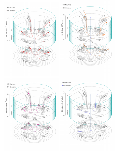
Figure S6: Developmental chrono-dendrograms for the Retrovesicular (G5, top left), Posterolateral (G6, top right), Preanal (G7, bottom left) and Dorsorectal (G8, bottom right) ganglia, showing that each comprises multiple localized clusters of neurons. Colored nodes represent neurons belonging to the specified ganglion while grey nodes show other neurons. Branching lines trace all cell divisions starting from the single cell zygote (located at the origin) and terminating at each differentiated neuron. The time and rung of each cell division is indicated by its position along the vertical and radial axis respectively. The entire time period is divided into four stages, viz., Embryo (indicated as E), L1, L2 and L3. A planar projection at the base of each cylinder shows the rung (concentric circles) of each progenitor cell and differentiated neuron.

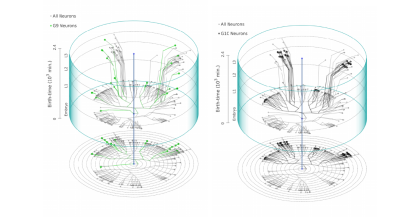
Figure S7: Developmental chrono-dendrograms for the Lumbar ganglion (G9, left) and the Ventral Cord (G10, right), showing that each comprises multiple localized clusters of neurons. Colored nodes represent neurons belonging to the specified ganglion while grey nodes show other neurons. Branching lines trace all cell divisions starting from the single cell zygote (located at the origin) and terminating at each differentiated neuron. The time and rung of each cell division is indicated by its position along the vertical and radial axis respectively. The entire time period is divided into four stages, viz., Embryo (indicated as E), L1, L2 and L3. A planar projection at the base of each cylinder shows the rung (concentric circles) of each progenitor cell and differentiated neuron.

References

- Lichtman et al. (2014) J. W. Lichtman, H. Pfister, and N. Shavit, Nature Neuroscience 17, 1448 (2014).
- Hassan and Hiesinger (2015) B. A. Hassan and P. R. Hiesinger, Cell 163, 285 (2015).
- Mitchell (2007) K. J. Mitchell, PLoS Biology 5, e113 (2007).
- Adolphs (2015) R. Adolphs, Trends in Cognitive Sciences 19, 173 (2015).
- Araújo and Tear (2003) S. J. Araújo and G. Tear, Nature Reviews Neuroscience 4, 910 (2003).
- Chen and Cheng (2009) S.-Y. Chen and H.-J. Cheng, Current Opinion in Neurobiology 19, 471 (2009).
- Colón-Ramos (2009) D. A. Colón-Ramos (Elsevier, 2009) pp. 53–79.
- Kolodkin and Tessier-Lavigne (2011) A. L. Kolodkin and M. Tessier-Lavigne, Cold Spring Harbor Perspectives in Biology 3, a001727 (2011).
- Kaiser (2017) M. Kaiser, Trends in Cognitive Sciences 21, 703 (2017).
- White et al. (1986) J. G. White, E. Southgate, J. N. Thomson, and S. Brenner, Philosophical Transactions of the Royal Society of London. B, Biological Sciences 314, 1 (1986).
- Varshney et al. (2011) L. R. Varshney, B. L. Chen, E. Paniagua, D. H. Hall, and D. B. Chklovskii, PLOS Computational Biology 7, e1001066 (2011).
- Brenner (2009) S. Brenner, Genetics 182, 413 (2009).
- Riddle et al. (1997) D. L. Riddle, T. Blumenthal, B. J. Meyer, and J. R. Priess, eds., C. elegans II, Cold Spring Harbor Monograph Series, Vol. 33 (Cold Spring Harbor Laboratory Press, Cold Spring Harbor, NY, 1997).
- Haag et al. (2018) E. S. Haag, D. H. A. Fitch, and M. Delattre, Genetics 210, 397 (2018).
- Hillier et al. (2005) L. W. Hillier, A. Coulson, J. I. Murray, Z. Bao, J. E. Sulston, and R. H. Waterston, Genome Research 15, 1651 (2005).
- Sulston and Horvitz (1977) J. E. Sulston and H. R. Horvitz, Developmental Biology 56, 110 (1977).
- Sulston et al. (1983) J. E. Sulston, E. Schierenberg, J. G. White, and J. N. Thomson, Developmental Biology 100, 64 (1983).
- Emmons (2016) S. W. Emmons, in Current Topics in Developmental Biology, Vol. 116 (Elsevier, 2016) pp. 315–330.
- Brenner (1974) S. Brenner, Genetics 77, 71 (1974).
- Culotti (1994) J. G. Culotti, Current Opinion in Genetics & Development 4, 587 (1994).
- Margeta et al. (2008) M. A. Margeta, K. Shen, and B. Grill, Current Opinion in Neurobiology 18, 69 (2008).
- Cherra and Jin (2015) S. J. Cherra and Y. Jin, WIREs Developmental Biology 4, 85 (2015).
- Goodhill (2016) G. J. Goodhill, Trends in Neurosciences 39, 202 (2016).
- Marr (1982) D. Marr, Vision: A Computational Investigation into the Human Representation and Processing of Visual Information (W. H. Freeman and Co., San Francisco, CA, 1982).
- Bassett et al. (2008) D. S. Bassett, E. Bullmore, B. A. Verchinski, V. S. Mattay, D. R. Weinberger, and A. Meyer-Lindenberg, Journal of Neuroscience 28, 9239 (2008).
- Bullmore and Sporns (2009) E. Bullmore and O. Sporns, Nature Reviews Neuroscience 10, 186 (2009).
- Park and Friston (2013) H.-J. Park and K. Friston, Science 342, 1238411 (2013).
- Stam (2014) C. J. Stam, Nature Reviews Neuroscience 15, 683 (2014).
- Fornito et al. (2015) A. Fornito, A. Zalesky, and M. Breakspear, Nature Reviews Neuroscience 16, 159 (2015).
- Schröter et al. (2017) M. Schröter, O. Paulsen, and E. T. Bullmore, Nature Reviews Neuroscience 18, 131 (2017).
- Reigl et al. (2004) M. Reigl, U. Alon, and D. B. Chklovskii, BMC Biology 2, 25 (2004).
- Chatterjee and Sinha (2007) N. Chatterjee and S. Sinha, Progress in Brain Research 168, 145 (2007).
- Pan et al. (2010) R. K. Pan, N. Chatterjee, and S. Sinha, PLOS ONE 5, e9240 (2010).
- Towlson et al. (2013) E. K. Towlson, P. E. Vértes, S. E. Ahnert, W. R. Schafer, and E. T. Bullmore, Journal of Neuroscience 33, 6380 (2013), http://www.jneurosci.org/content/33/15/6380.full.pdf .
- Varier and Kaiser (2011) S. Varier and M. Kaiser, PLOS Computational Biology 7, e1001044 (2011).
- Alicea (2018) B. Alicea, Biosystems 173, 247 (2018).
- Ahn et al. (2006) Y.-Y. Ahn, H. Jeong, and B. J. Kim, Physica A: Statistical Mechanics and its Applications 367, 531 (2006).
- Chen et al. (2006) B. L. Chen, D. H. Hall, and D. B. Chklovskii, Proceedings of the National Academy of Sciences USA 103, 4723 (2006), https://www.pnas.org/content/103/12/4723.full.pdf .
- Pérez-Escudero and de Polavieja (2007) A. Pérez-Escudero and G. G. de Polavieja, Proceedings of the National Academy of Sciences USA 104, 17180 (2007).
- Rivera-Alba et al. (2014) M. Rivera-Alba, H. Peng, G. G. de Polavieja, and D. B. Chklovskii, Current Biology 24, R109 (2014).
- Gushchin and Tang (2015) A. Gushchin and A. Tang, PLOS ONE 10, e0145029 (2015).
- Wang and Clandinin (2016) I. E. Wang and T. R. Clandinin, Current Biology 26, R1101 (2016).
- Chalfie et al. (1985) M. Chalfie, J. E. Sulston, J. G. White, E. Southgate, J. N. Thomson, and S. Brenner, Journal of Neuroscience 5, 956 (1985).
- Wicks and Rankin (1995) S. R. Wicks and C. H. Rankin, Journal of Neuroscience 15, 2434 (1995).
- Sawin (1996) E. R. Sawin, Genetic and cellular analysis of modulated behaviors in Caenorhabditis elegans, Ph.D. thesis, Massachusetts Institute of Technology, Cambridge, Massachusetts (1996).
- Troemel et al. (1997) E. R. Troemel, B. E. Kimmel, and C. I. Bargmann, Cell 91, 161 (1997).
- Kaiser and Hilgetag (2006) M. Kaiser and C. C. Hilgetag, PLOS Computational Biology 2, e95 (2006).
- Newman, Mark E.J. (2004) Newman, Mark E.J., Eur. Phys. J. B 38, 321 (2004).
- Newman (2010) M. E. Newman, Networks: An Introduction (Oxford University Press, Oxford, 2010).
- Pfister et al. (2013) R. Pfister, K. A. Schwarz, M. Janczyk, R. Dale, and J. Freeman, Frontiers in Psychology 4, 700 (2013).
- Xu et al. (2018) T. Xu, J. Huo, S. Shao, M. Po, T. Kawano, Y. Lu, M. Wu, M. Zhen, and Q. Wen, Proceedings of the National Academy of Sciences USA 115, E4493 (2018).
- Hall (2017) D. H. Hall, Developmental Neurobiology 77, 587 (2017).
- Wood (1988) W. B. Wood, ed., The Nematode Caenorhabditis Elegans, Cold Spring Harbor Monograph Series, Vol. 17 (Cold Spring Harbor Laboratory Press, Cold Spring Harbor, NY, 1988).
- Giurumescu and Chisholm (2011) C. A. Giurumescu and A. D. Chisholm, in Methods in Cell Biology, Vol. 106, edited by J. H. Rothman and A. Singson (Elsevier, Waltham, MA, 2011) pp. 323–341.
- Schafer (2016) W. Schafer, Current Biology 26, R955 (2016).
- Tessier-Lavigne and Goodman (1996) M. Tessier-Lavigne and C. S. Goodman, Science 274, 1123 (1996).
- Hobert (2014) O. Hobert, Genesis 52, 528 (2014).
- Hobert (2005) O. Hobert, in WormBook, edited by T. C. elegans Research Community (www.wormbook.org, 2005).
- Hobert et al. (2002) O. Hobert, R. J. Johnston Jr, and S. Chang, Nature Reviews Neuroscience 3, 629 (2002).
- Tolstenkov et al. (2018) O. Tolstenkov, P. Van der Auwera, W. S. Costa, O. Bazhanova, T. M. Gemeinhardt, A. C. F. Bergs, and A. Gottschalk, eLife 7, e34997 (2018).
- Guimerà and Amaral (2005a) R. Guimerà and L. A. N. Amaral, nature 433, 895 (2005a).
- Guimerà and Amaral (2005b) R. Guimerà and L. A. N. Amaral, Journal of Statistical Mechanics: Theory and Experiment 2005, P02001 (2005b).
- Waggoner et al. (1998) L. E. Waggoner, G. T. Zhou, R. W. Schafer, and W. R. Schafer, Neuron 21, 203 (1998).
- Bany et al. (2003) I. A. Bany, M.-Q. Dong, and M. R. Koelle, Journal of Neuroscience 23, 8060 (2003).
- Mori and Ohshima (1995) I. Mori and Y. Ohshima, Nature 376, 344 (1995).
- Gray et al. (2005) J. M. Gray, J. J. Hill, and C. I. Bargmann, Proceedings of the National Academy of Sciences USA 102, 3184 (2005).
- Wicks and Rankin (1996) S. R. Wicks and C. H. Rankin, Journal of Comparative Physiology A 179, 675 (1996).
- Bargmann (2012) C. I. Bargmann, Bioessays 34, 458 (2012).
- Bentley et al. (2016) B. Bentley, R. Branicky, C. L. Barnes, Y. L. Chew, E. Yemini, E. T. Bullmore, P. E. Vértes, and W. R. Schafer, PLoS Computational Biology 12, e1005283 (2016).
- Wolpert and Tickle (2011) L. Wolpert and C. Tickle, Principles of Development (4th Edition) (Oxford University Press, 2011).
- Easley and Kleinberg (2010) D. Easley and J. Kleinberg, Networks, Crowds, and Markets: Reasoning about a highly connected world (Cambridge University Press, Cambridge, 2010).
- Davidsen et al. (2002) J. Davidsen, H. Ebel, and S. Bornholdt, Physical Review Letters 88, 128701 (2002).
- Brot et al. (2015) H. Brot, L. Muchnik, and Y. Louzoun, The European Physical Journal B 88, 12 (2015).
- Azulay et al. (2016) A. Azulay, E. Itskovits, and A. Zaslaver, PLoS Computational Biology 12, e1005021 (2016).
- WormAtlas et al. (2019) WormAtlas, Z. F. Altun, L. A. Herndon, C. A. Wolkow, C. Crocker, R. Lints, and D. H. Hall, A database featuring behavioural and structural anatomy of caenorhabditis elegans (2002-2019).
- Bhatla (2011) N. Bhatla, An interactive visualization of the c. elegans cell lineage (2011).
- Choe et al. (2004) Y. Choe, B. H. McCormick, and W. Koh, in Soc. Neurosci. Abstr., Vol. 30 (2004).
- Achacoso and Yamamoto (1991) T. B. Achacoso and W. S. Yamamoto, AY’s Neuroanatomy of C. Elegans for Computation, 1st ed. (CRC Press, Boca Raton, FL, 1991).
- Massey (1951) F. J. Massey, Journal of the American Statistical Association 46, 68 (1951).
- Bowman and Azzalini (1997) A. W. Bowman and A. Azzalini, Applied Smoothing Techniques for Data Analysis: The Kernel Approach with S-PLUS Illustrations (Oxford University Press, Oxford, 1997).
SUPPLEMENTARY MATERIAL