Ab Initio Path Integral Monte Carlo Approach
to the Static and Dynamic Density Response of the Uniform Electron Gas

Abstract

In a recent Letter [T. Dornheim et al., Phys. Rev. Lett. 121, 255001 (2018)] we have presented the first ab initio results for the dynamic structure factor $S(\mathbf{q},\omega)$ of the uniform electron gas for conditions ranging from the warm dense matter regime to the strongly correlated electron liquid. This was achieved on the basis of exact path integral Monte Carlo data by stochastically sampling the dynamic local field correction $G(\mathbf{q},\omega)$. In this paper, we introduce in detail this new reconstruction method and provide several practical demonstrations. Moreover, we thoroughly investigate the associated imaginary-time density–density correlation function $F(\mathbf{q},\tau)$. The latter also gives us access to the static density-response function $\chi(\mathbf{q})$ and static local field correction $G(\mathbf{q})$, which are compared to standard dielectric theories like the widespread random phase approximation. In addition, we study the high-frequency limit of $G(\mathbf{q},\omega)$ and provide extensive new results for the dynamic structure factor for different densities and temperatures. Finally, we discuss the implications of our findings for warm dense matter research and the interpretation of experiments.

I Introduction

The uniform electron gas (UEG) is one of the most important model systems in physics and quantum chemistry quantum_theory ; loos . First and foremost, it was only the accurate parametrization of the exchange-correlation energy of the UEG vwn ; perdew based on zero-temperature quantum Monte Carlo (QMC) calculations gs1 ; gs2 that facilitated the spectacular success of density functional theory simulations of real materials dft_review . Moreover, the UEG has been of paramount importance for several breakthroughs in theoretical physics such as Fermi liquid theory pines or the Bardeen-Cooper-Schrieffer theory of superconductivity bcs ; bcs2 .

While most static properties of the UEG have been known at zero temperature for decades, there recently has emerged a growing interest into the properties of electrons at extreme densities and temperatures ross ; koenig ; fortov_review . In fact, this so-called warm dense matter (WDM) regime constitutes one of the most active frontiers in plasma physics and is of fundamental importance for, e.g., the description of astrophysical objects like giant planet interiors militzer1 ; militzer2 ; knudson ; militzer3 ; manuel and brown dwarfs saumon1 ; saumon2 ; becker , laser-excited solids ernstorfer2 ; ernstorfer , and the pathway towards inertial confinement fusion nora ; schmit ; hurricane3 ; kritcher —the latter potentially offering a near abundance of clean energy in the future. In addition, WDM is now routinely realized in experiments with, e.g., free-electron lasers lcls1 ; sperling ; xfel1 or diamond anvil cells benuzzi in large research facilities around the globe, see Ref. falk_wdm for a topical overview.

From a theoretical perspective, the WDM regime is defined by two parameters that are both of the order of unity: 1) the density parameter (sometimes denoted as quantum coupling parameter or Wigner-Seitz-radius) $r_{s}=\overline{r}/a_{\textnormal{B}}$, with $\overline{r}$ and $a_{\textnormal{B}}$ being the average inter-particle distance and Bohr radius, and 2) the degeneracy temperature $\theta=k_{\textnormal{B}}T/E_{\textnormal{F}}$, with $E_{\textnormal{F}}$ being the Fermi energy. Strictly speaking, a third parameter is given by the classical coupling parameter $\Gamma=Ze^{2}/(\overline{r}k_{\textnormal{B}}T)\sim 1$ describing the ionic component in real WDM systems, but it is of no relevance for the UEG and, therefore, is not further discussed in the present work.

Speaking in terms of physical effects, WDM is characterized by the intriguingly intricate interplay of the Coulomb repulsion between the electrons with thermal excitations and quantum degeneracy effects, such as quantum diffraction and Pauli blocking. Moreover, there are no small parameters to conduct an expansion around, which leaves numerical methods as the only option, with QMC approaches being particularly promising wdm_book . This renders WDM theory a notoriously tricky business, as QMC simulations of electrons are severely hampered by the infamous fermion sign problem (FSP) dornheim_pop ; troyer ; loh . Consequently, despite intensive efforts regarding the warm dense UEG over several decades pines ; kugler1 ; F ; ebeling ; stls ; rajagopal ; pdw ; stolzmann ; sandipan ; brown_ethan ; vladimir_UEG ; dornheim_test , the accurate description of this system has only been achieved recently. In particular, Groth, Dornheim and co-workers groth_prl ; review have presented an accurate parametrization of the exchange-correlation free energy $f_{\textnormal{XC}}$ of the warm dense UEG on the basis of different path integral Monte Carlo (PIMC) techniques dornheim ; groth ; dornheim2 ; dornheim3 ; dornheim_prl ; dornheim_neu , which is available over the entire relevant parameter range and provides a full thermodynamic description, see Ref. review for a topical review article.

In spite of these significant advances, one crucial piece of the bigger puzzle that is the theory of the warm dense electron gas is yet missing: the response of an electron gas to an external perturbation. In particular, the experimental observation and subsequent theoretical description of the time-dependent density response is of paramount importance as a method of diagnostics in modern WDM applications siegfried_review ; valenzuela ; dominik . In this context, the central quantity is given by the dynamic density–density response function $\chi(\mathbf{q},\omega)$, with $\mathbf{q}$ and $\omega$ being the wave vector and frequency, or, equivalently, the dynamic structure factor $S(\mathbf{q},\omega)$, that is directly measured in X-ray Thomson scattering experiments, see Ref. siegfried_review for a review. In addition to its utility for the interpretation of experiments, the dynamic density-response is important as input for many nonequilibrium applications such as the stopping power Cayzac:2017 ; Fu:2017 , energy transfer rates and relaxation transfer1 ; transfer2 , electrical and thermal conductivities Desjarlais:2017 ; Veysman:2016 , quantum hydrodynamics zhandos , or the development of advanced exchange–correlation functionals for density function theory lu ; patrick ; burke2 .

Unfortunately, an exact theory for $\chi(\mathbf{q},\omega)$ is even more challenging than for the previously discussed static properties, as one, in principle, would have to carry out an explicit propagation in time. Needless to say, this is in general not possible for an interacting quantum many-body system except in a few limiting cases. Consequently, the dynamic density response is relatively poorly understood even in the ground state, see Refs. takada1 ; takada2 for the presumably most accurate data. Moreover, ab initio QMC methods are limited to the description of the static limit bowen ; moroni [i.e., a constant, time-independent external perturbation described by $\chi(\mathbf{q})=\chi(\mathbf{q},\omega=0)$], and even this task has turned out to be relatively expensive and QMC data are only available at a few selected parameters moroni2 ; bowen2 . For completeness, we mention that this approach has recently been adapted to the WDM regime in Refs. dornheim_pre ; groth_jcp , but here the available data points have remained even more sparse.

On the other hand, it has long been known that PIMC methods berne1 ; berne2 allow for a straightforward calculation of the imaginary-time density–density correlation function $F(\mathbf{q},\tau)$, cf. Eq. (15) below. In addition to direct access to the static density response, this quantity can be used as input for the reconstruction of $S(\mathbf{q},\omega)$, which is a well known, but notoriously difficult problem jarrell ; schoett . In particular, the obtained solution for $S(\mathbf{q},\omega)$ are often not unique since the PIMC data for $F$ are afflicted with a statistical uncertainty, and one somehow has to provide additional input to render the reconstruction tractable. Indeed, we have recently dornheim_dynamic proposed a novel reconstruction procedure based on the stochastic sampling of the dynamic local field correction (LFC) $G(\mathbf{q},\omega)$, which allows to automatically fulfill a number of exact constraints. This, in turn, has allowed us to present the first accurate data for $S(\mathbf{q},\omega)$ of the UEG going from the WDM regime to the strongly correlated electron liquid.

In this paper, we further explore this new procedure and present in detail the involved theory, provide practical examples, and give extensive new data both for static and dynamic quantities for hitherto unexplored parameters. In addition to the value of our results for the description of matter under extreme conditions, we expect our new reconstruction procedure to be of broad interest for different communities, such as ultracold bosonic atoms dynamic_alex1 ; dynamic_alex2 ; vitali ; supersolid or condensed matter physics gull ; som ; igorrr .

The paper is organised as follows: in Sec. II, we introduce the required theory, starting with the utilized path integral Monte Carlo method (II.1) and linear response theory (II.2). Furthermore, we introduce the concept of imaginary-time correlation-functions and their relation to the dynamic structure factor (II.3), the general problem of reconstruction (II.4), and our new stochastic sampling procedure (II.5) based on the dynamic LFC. The discussion of our results in Sec. III starts with an investigation of $F(\mathbf{q},\tau)$ (III.1), followed by the static properties of the UEG (III.2), and the respective high-frequency ($\omega\to\infty$) limit. In Sec. III.3, we present two practical examples of the reconstruction of $S(\mathbf{q},\omega)$ and subsequently (III.4) give new results for previously unexplored conditions. The paper is concluded by a brief summary and discussion in Sec. IV.

We assume Hartree atomic units throughout this work.

II Theory

II.1 Path Integral Monte Carlo

Let us consider a system of $N$ unpolarized electrons (i.e., with identical numbers of spin-up and -down electrons, $N_{\uparrow}=N_{\downarrow}=N/2$) in a volume $V=L^{3}$ at an inverse temperature $\beta=1/k_{\textnormal{B}}T$. In this case, all thermodynamic observables can be computed from the canonical partition function, which, in coordinate space, is given by

$$Z = \frac{1}{N_{\uparrow}!N_{\downarrow}!}\sum_{\sigma_{\uparrow}\in S_{N_{\uparrow}}}\sum_{\sigma_{\downarrow}\in S_{N_{\downarrow}}}\textnormal{sgn}^{\textnormal{f}}(\sigma_{\uparrow},\sigma_{\downarrow})$$

$$\int\textnormal{d}\mathbf{R}\ \bra{\mathbf{R}}e^{-\beta\hat{H}}\ket{\hat{\pi}_{\sigma_{\uparrow}}\hat{\pi}_{\sigma_{\downarrow}}\mathbf{R}}\quad,$$

with $\sigma_{i}$ denoting a particular element from the permutation group $S_{N_{i}}$, and $\hat{\pi}_{\sigma_{i}}$ being the corresponding permutation operator with $i\in\{\uparrow,\downarrow\}$. Observe that in this notation $\mathbf{R}$ contains the coordinates of both spin-up and -down electrons, and the sign function $\textnormal{sgn}^{\textnormal{f}}(\sigma_{\uparrow},\sigma_{\downarrow})$ can be positive or negative depending on the number of pair-exchanges. The problem with Eq. (II.1) is that the matrix elements of the density operator $\hat{\rho}=e^{-\beta\hat{H}}$ cannot be evaluated as the kinetic and potential contributions, $\hat{K}$ and $\hat{V}$, do not commute, i.e.,

$$e^{-\beta\hat{H}}=e^{-\beta\hat{K}}e^{-\beta\hat{V}}+\mathcal{O}\left(\beta^{2}\right)\quad.$$ (2)

The basic idea of the path integral Monte Carlo formalism berne3 ; cep is to perform a Trotter decomposition trotter and express the partition function as the sum over $P$ sets of particle coordinates, but evaluated at a $P$-times higher temperature,

$$Z = \frac{1}{N_{\uparrow}!N_{\downarrow}!}\sum_{\sigma_{\uparrow}\in S_{N_{\uparrow}}}\sum_{\sigma_{\downarrow}\in S_{N_{\downarrow}}}\textnormal{sgn}^{\textnormal{f}}(\sigma_{\uparrow},\sigma_{\downarrow})$$

$$\int\textnormal{d}\mathbf{R}_{0}\dots\textnormal{d}\mathbf{R}_{P-1}\prod_{\alpha=0}^{P-1}\bra{\mathbf{R}_{\alpha}}e^{-\epsilon\hat{H}}\ket{\hat{\pi}_{P-1}\mathbf{R}_{\alpha-1}}$$

$$= \int\textnormal{d}\mathbf{X}\ W(\mathbf{X})\quad,$$

with $\epsilon=\beta/P$ and $\hat{\pi}_{P-1}$ only having an effect for $\alpha=P-1$. Evidently, the factorization error from Eq. (2) can be made arbitrarily small by increasing the convergence parameter $P$, which in turn means that any desired level of accuracy can be realized and the PIMC formalism is quasi-exact. Note that the sign $\textnormal{sgn}^{\textnormal{f}}(\sigma_{\uparrow},\sigma_{\downarrow})$ depends on the parity of a particular permutation of particle coordinates and flips for every pair-exchange. Further, it holds $\mathbf{R}_{0}=\mathbf{R}_{P-1}$, which implies that Eq. (II.1) can be interpreted as the sum over all closed paths $\mathbf{X}$ of particle coordinates in the so-called imaginary-time $\tau=-i\hbar\beta$.

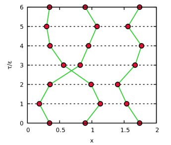
Figure 1: Schematic illustration of Path Integral Monte Carlo—Shown is a configuration of $N=3$ electrons with $P=6$ imaginary–time propagators in the $x$-$\tau$ plane. Due to the single pair-exchange, the corresponding configuration weight $W(\mathbf{X})$ is negative.

This is illustrated in Fig. 1, where we show a configuration of $N_{\uparrow}=3$ electrons in the $x$-$\tau$-plane. In this particular example, we are having $P=6$ imaginary-time slices, with the coordinates at $\alpha=0$ and $\alpha=6$ being identical. In addition, the corresponding configuration weight $W(\mathbf{X})$ is negative due to the presence of a single pair-exchange. Moreover, each high-temperature factor can be viewed as a propagation in the imaginary time by a time-step $\epsilon$, which allows for straightforward measurements of imaginary-time correlation-functions as discussed in Sec. II.3.

The basic idea of the PIMC approach is to use the Metropolis algorithm metropolis to stochastically sample the paths $\mathbf{X}$ according to $W(\mathbf{X})$. Unfortunately, however, this is not directly possible as $W(\mathbf{X})$ is not strictly positive and, thus, cannot be interpreted as a probability distribution. To circumvent this issue, we consider the modified partition function

$$Z^{\prime}=\int\textnormal{d}\mathbf{X}\ |W(\mathbf{X})|\quad,$$ (4)

and the exact fermionic expectation value of interest can then be computed as

$$\langle O\rangle=\frac{\langle OS\rangle^{\prime}}{\langle S\rangle^{\prime}}\quad,$$ (5)

with averages being carried out over the modified distribution $W^{\prime}(\mathbf{X})=|W(\mathbf{X})|$ and $S=W(\mathbf{X})/|W(\mathbf{X})|=\textnormal{sgn}^{\textnormal{f}}(\sigma_{\uparrow},\sigma_{\downarrow})$ denoting the sign. In practice, both the enumerator and denominator in Eq. (5) vanish simultaneously with increasing system size and decreasing temperature. This leads to an exponentially increasing statistical uncertainty (error bar), which is nothing else than the notorious fermion sign problem loh ; troyer . In fact, the FSP constitutes the paramount obstacle in our simulations and prevents PIMC simulations of the UEG for lower temperatures and higher densities, i.e., in the regime where quantum degeneracy effects dominate dornheim_pop ; review .

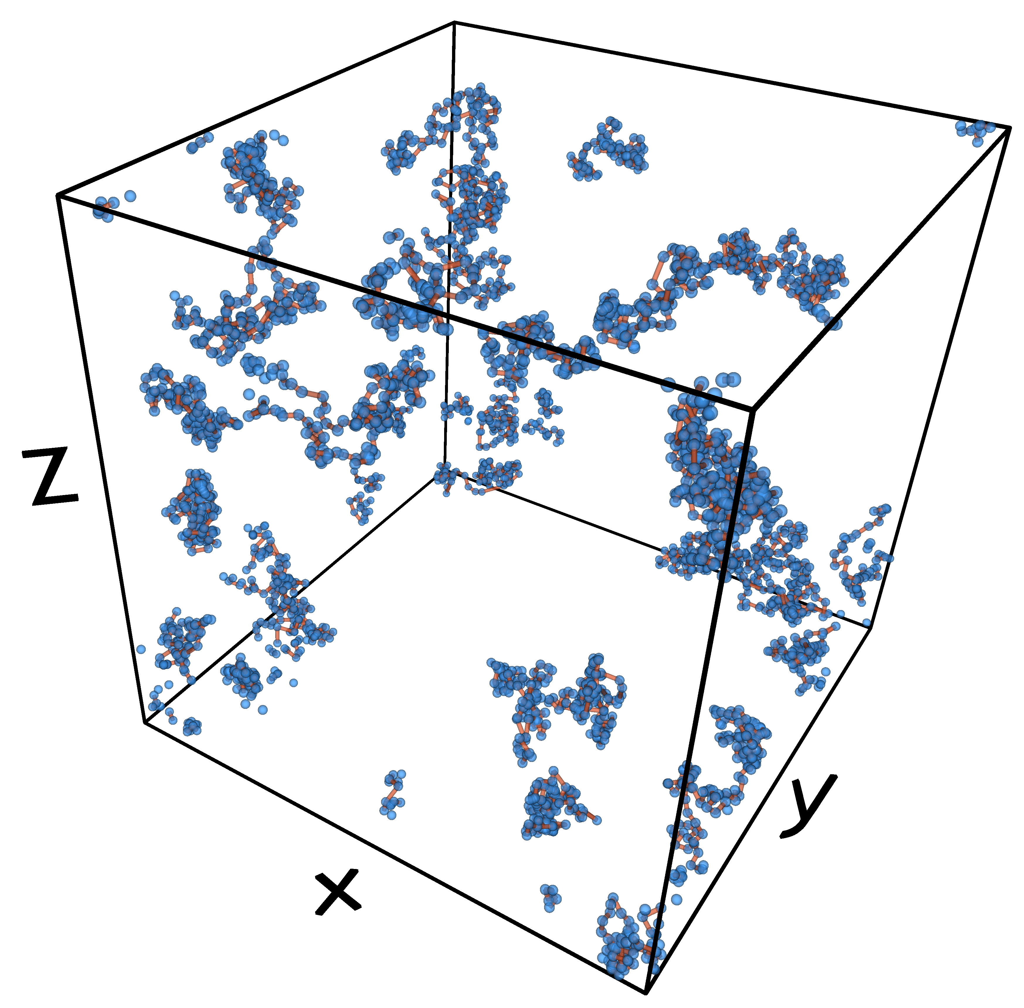
Figure 2: Snapshot of a PIMC simulation of the UEG at $r_{s}=1$ and $\theta=1$ with $N=17$ and $P=100$.

In Fig. 2 we show a snapshot from a PIMC simulation of $N=17$ electrons at $r_{s}=1$ and $\theta=1$ with $P=100$ imaginary-time slices. Note that we use an adaption of the worm algorithm by Boninsegni et al. boninsegni1 ; boninsegni2 throughout this work. Evidently, there are many permutations of particle coordinates present (see also the recent discussion of permutation properties in Ref. dornheim_permutation ) at these warm dense matter conditions and the sign of $W(\mathbf{X})$ within a simulation frequently changes. The resulting cancellation of positive and negative terms drastically increases the statistical uncertainty, which often cannot be compensated for by increasing the computation time, see Refs. review ; dornheim_pop for a more extensive discussion.

For completeness, we mention that the more advanced permutation blocking PIMC dornheim ; dornheim2 and configuration PIMC groth ; dornheim3 methods are capable to provide accurate results for static properties of the UEG when PIMC breaks down due to the sign problem. Unfortunately, however, the imaginary-time density-correlation function $F(\mathbf{q},\tau)$, which is of central importance in this work, can at present not be computed from these new techniques, so that PIMC remains the method of choice here.

II.2 Linear response theory

Let us next consider the effect of a small, time-dependent external perturbation, $\hat{H}_{A}(t)$,

$$\hat{H}(t)=\hat{H}_{\textnormal{UEG}}+\hat{H}_{A}(t)\quad,$$ (6)

with $\hat{H}_{\textnormal{UEG}}$ being the static UEG Hamiltonian. Note that we employ the standard Ewald summation as described in, e.g., Ref. fraser . In particular, we consider a sinusoidal charge density of the form

$$\hat{H}_{A}(t)=2A\sum_{i=1}^{N}\textnormal{cos}(\mathbf{r}_{i}\cdot\mathbf{q}-\Omega t)\quad,$$ (7)

with the wave vector $\mathbf{q}$, frequency $\Omega$, and perturbation amplitude $A$. Within linear response theory quantum_theory , which is accurate for sufficiently small perturbations, the response of the UEG to Eq. (7) is fully described by the density response function

$$\tilde{\chi}(\mathbf{q},\overline{t})=-\frac{i}{\hbar}\braket{[\rho(\mathbf{q},t),\rho(-\mathbf{q},t^{\prime})]}\quad,$$ (8)

where the expectation value $\braket{\dots}$ has to be carried out with respect to the unperturbed Hamiltonian, i.e., $\hat{H}_{\textnormal{UEG}}$. Therefore, Eq. (8) only depends on the relative difference between the time arguments, $\overline{t}=t-t^{\prime}$, and on the modulus of the wave number $q=|\mathbf{q}|$. We note that it is often more convenient to work in frequency space, and a straightforward Fourier transform gives

$$\chi(\mathbf{q},\omega)=\lim_{\eta\to 0}\int_{-\infty}^{\infty}\textnormal{d}\overline{t}\ e^{(i\omega-\eta)\overline{t}}\tilde{\chi}(\mathbf{q},\overline{t})\quad.$$ (9)

For completeness, we explicitly define the static density-response function,

$$\chi(\mathbf{q})=\lim_{\omega\to 0}\chi(\mathbf{q},\omega)\quad,$$ (10)

which describes the response of the UEG to a constant (i.e., time independent) external charge.

II.3 Dynamic structure factor and imaginary-time correlation functions

A central quantity in modern WDM research (and many other fields) is the so-called dynamic structure factor,

$$S(\mathbf{q},\omega)=\frac{1}{2\pi N}\int_{-\infty}^{\infty}\textnormal{d}t\ \braket{\rho(\mathbf{q},t)\rho(-\mathbf{q},0)}e^{i\omega t}\quad,$$ (11)

which is directly accessible in XRTS experiments siegfried_review and is of paramount importance for diagnostics like, e.g., the determination of the electronic temperature within a sample dominik . We note that Eq. (11) obeys the detailed balance condition

$$S(\mathbf{q},\omega)=S(\mathbf{q},-\omega)e^{-\beta\omega}\quad,$$ (12)

so that the consideration of the positive frequency range is sufficient. In addition, $S(\mathbf{q},\omega)$ is directly connected to the imaginary part of the dynamic density-response function from the previous section by the fluctuation–dissipation theorem

$$S(\mathbf{q},\omega)=-\frac{\textnormal{Im}\chi(\mathbf{q},\omega)}{\pi n(1-e^{-\beta\omega})}\quad.$$ (13)

Evidently, $S(\mathbf{q},\omega)$ is nothing else than the Fourier transform of the intermediate scattering function

$$F(\mathbf{q},t)=\frac{1}{N}\braket{\rho(\mathbf{q},t)\rho(-\mathbf{q},0)}\quad,$$ (14)

and, in principle, requires an explicitly time-dependent theoretical description, which is notoriously difficult and almost unfeasible in the presence of correlation effects.

A neat alternative is given by the analytic continuation of the imaginary-time density correlation function, which is defined as

$$F(\mathbf{q},\tau)=\frac{1}{N}\braket{\rho(\mathbf{q},\tau)\rho(-\mathbf{q},0)}\quad.$$ (15)

Although Eq. (15) is formally obtained by a propagation in imaginary-time by $\tau=-i\hbar\beta$, the pre-factors are usually dropped such that $\tau\in[0,\beta]$; this convention is applied throughout the remainder of this paper. The crucial point in the context of the present work is that $F(\mathbf{q},\tau)$ is directly accessible within our PIMC simulations in thermodynamic equilibrium berne1 ; berne2 by measuring the correlation between the Fourier components of the density operator on different imaginary-time slices, see Fig. 1 for a graphical depiction. The connection of $F$ to the dynamic structure factor is then given by a Laplace transform

$$F(\mathbf{q},\tau)=\int_{-\infty}^{\infty}\textnormal{d}\omega\ S(\mathbf{q},\omega)e^{-\tau\omega}\quad.$$ (16)

Therefore, the task at hand is to numerically solve Eq. (16) by performing an inverse Laplace transform, which is a well-known but ill-posed problem jarrell .

II.4 Reconstruction of the dynamic structure factor

The central obstacle regarding the reconstruction of the dynamic structure factor from an imaginary-time correlation function is the statistical uncertainty in the corresponding QMC data. Therefore, there are potentially infinitely many valid trial solutions $S_{\textnormal{trial}}(\mathbf{q},\omega)$, which, when being inserted into Eq. (16), perfectly reproduce the Monte Carlo data within the given error bars. Typically, these $S_{\textnormal{trial}}(\mathbf{q},\omega)$ are very noisy (sawtooth instability) and often plainly unphysical. Hence, additional constraints on the trial solutions are indispensable to obtain reliable structure factors on the basis of our PIMC data.

A commonly used type of information are frequency moments of the form

$$\braket{\omega^{k}}=\int_{-\infty}^{\infty}\textnormal{d}\omega\ S(\mathbf{q},\omega)\ \omega^{k}\quad,$$ (17)

where, in the case of the UEG, four different cases are known:

1. The inverse moment is determined by the static density response function iwamoto2 ; pines_woo ; kugler2

   $$\braket{\omega^{-1}}=-\frac{\chi(\mathbf{q})}{2n}\quad,$$ (18)

   see also Eq. (10). Conveniently, $\chi(\mathbf{q})$ is straightforwardly obtained from $F(\mathbf{q},\tau)$ via the imaginary-time analogue of the fluctuation–dissipation theorem, which states that bowen ; alex_prok

   $$\chi(\mathbf{q})=-n\int_{0}^{\beta}\textnormal{d}\tau\ F(\mathbf{q},\tau)\quad.$$ (19)

2. The normalization, or zero-moment, is given by the static structure factor

   $$\braket{\omega^{0}}=\int_{-\infty}^{\infty}\textnormal{d}\omega\ S(\mathbf{q},\omega)=:S(\mathbf{q})\quad.$$ (20)

   Note that $S(\mathbf{q})$ is defined as the integral over $S(\mathbf{q},\omega)$ and not as the static limit as in the case of $\chi(\mathbf{q})$ and $\chi(\mathbf{q},\omega)$.

3. The first moment is known analytically from the f sum-rule quantum_theory ,

   $$\braket{\omega^{1}}=\frac{q^{2}}{2}\quad.$$ (21)

4. The third moment was first reported in Refs. puff1 ; puff2 and reads iwamoto2 ; iwamoto ; quantum_theory

   $$\braket{\omega^{3}}=\frac{q^{2}}{2}\Bigg{(} \Big{(} \frac{q^{2}}{2}\Big{)}^{2}+q^{2}nv_{q}+2q^{2}K$$

   $$+ \omega_{p}^{2}\big{(}1-I(q)\big{)}\Bigg{)}\quad,$$

   with $K$ being the mean kinetic energy of the correlated system, and where the potential contribution iwamoto ; quantum_theory can be expressed in spherical coordinates as a one-dimensional integral,

   $$I(q) = \frac{1}{8\pi^{2}n}\int_{0}^{\infty}\textnormal{d}k\ k^{2}\big{(}1-S(k)\big{)}$$

   $$\times \Bigg{(}\frac{5}{3}-\frac{k^{2}}{q^{2}}+\frac{\big{(}k^{2}-q^{2}\big{)}^{2}}{2kq^{3}}\textnormal{log}\Bigg{|}\frac{k+q}{k-q}\Bigg{|}\Bigg{)}\quad,$$

   which is evaluated numerically from spline-fits to $S(\mathbf{q})$, see also Refs. dornheim_prl ; dornheim_cpp for an extensive discussion.

While accurate knowledge of the $\braket{\omega^{k}}$ are known to significantly increase the quality of the reconstructed dynamic structure factors for some examples such as ultracold atoms dynamic_alex1 ; dynamic_alex2 , they have been proven to be insufficient to determine sufficiently constrained $S_{\textnormal{trial}}(\mathbf{q},\omega)$ for the UEG in many cases.

II.5 Stochastic sampling of the dynamic local field correction

To derive additional constraints on the reconstructed dynamic structure factors, we consider the fluctuation–dissipation theorem, Eq. (13), and express $\chi(\mathbf{q},\omega)$ in terms of a dynamic local field correction kugler1 ; quantum_theory ; gross ; dabrowski $G(\mathbf{q},\omega)$

$$\chi(\mathbf{q},\omega)=\frac{\chi_{0}(\mathbf{q},\omega)}{1-4\pi/q^{2}\big{[}1-G(\mathbf{q},\omega)\big{]}\chi_{0}(\mathbf{q},\omega)}\quad.$$ (24)

The dynamic density-response function of the noninteracting system, $\chi_{0}(\mathbf{q},\omega)$, is readily known, and all exchange-correlation effects regarding the density response are contained in $G$. Therefore, setting $G=0$ corresponds to the random phase approximation, which describes the response on a mean-field level. In a nutshell, the combination of Eqs. (13) and (24) implies that we have re-cast the reconstruction problem from a quest for $S(\mathbf{q},\omega)$ into a quest for the DLFC. This is extremely advantageous, as many additional exact properties of $G$ are known:

1. The Kramers-Kronig relations provide a connection between the real and imaginary parts of $G(\mathbf{q},\omega)$ kugler1 :

   $$\textnormal{Re}G(\mathbf{q},\omega) = \textnormal{Re}G(\mathbf{q},\infty)+\frac{1}{\pi}\int_{-\infty}^{\infty}\textnormal{d}\overline{\omega}\ \frac{\textnormal{Im}G(\mathbf{q},\overline{\omega})}{\overline{\omega}-\omega}$$ (25)

   $$\textnormal{Im}G(\mathbf{q},\omega) =$$

   $$- \frac{1}{\pi}\int_{-\infty}^{\infty}\textnormal{d}\overline{\omega}\ \frac{\textnormal{Re}G(\mathbf{q},\overline{\omega})-\textnormal{Re}G(\mathbf{q},\infty)}{\overline{\omega}-\omega}\quad.$$

2. $\textnormal{Re}G(\mathbf{q},\omega)$ and $\textnormal{Im}G(\mathbf{q},\omega)$ are even and odd functions with respect to $\omega$, respectively gross .

3. $\textnormal{Im}G(\mathbf{q},\omega)$ vanishes in the limits of high and low frequency gross :

   $$\textnormal{Im}G(\mathbf{q},0)=\textnormal{Im}G(\mathbf{q},\infty)=0\quad.$$ (27)

4. The static limit of $\textnormal{Re}G(\mathbf{q},\omega)$ is defined by static density response function [see Eq. (19)], since $\chi(\mathbf{q})$ is a real function quantum_theory :

   $$\textnormal{Re}G(\mathbf{q},0)=1-\frac{1}{v_{q}}\left(\frac{1}{\chi_{0}(\mathbf{q},0)}-\frac{1}{\chi(\mathbf{q})}\right)\quad.$$ (28)

   The high-frequency limit of $\textnormal{Re}G(\mathbf{q},\omega)$ can be computed from the static structure factor $S(\mathbf{q})$ and the exchange-correlation contribution to the kinetic energy, $K_{\textnormal{xc}}$,

   $$\textnormal{Re}G(\mathbf{q},\infty)=I(q)-\frac{2q^{2}K_{\textnormal{xc}}}{\omega_{p}^{2}}\quad.$$ (29)

   The interaction contribution $I(q)$ has been defined in Eq. (4), and $K_{\textnormal{xc}}$ can be computed from the exchange-correlation free energy $f_{\textnormal{xc}}$ via

   $$K_{\textnormal{xc}} = -f_{\textnormal{xc}}(r_{s},\theta)-\theta\frac{\partial f_{\textnormal{xc}}(r_{s},\theta)}{\partial\theta}\Bigg{|}_{r_{s}}$$

   $$-r_{s}\frac{\partial f_{\textnormal{xc}}(r_{s},\theta)}{\partial r_{s}}\Bigg{|}_{\theta}\quad.$$

   In practice, we are using the accurate recent parametrization of $f_{\textnormal{xc}}$ by Groth, Dornheim and co-workers (see Refs. groth_prl ; review ) to evaluate Eq. (4).

The basic idea of our new reconstruction method is to stochastically sample trial solutions $G_{\textnormal{trial}}(\mathbf{q},\omega)$, which automatically fulfill all aforementioned exact properties. These DLFCs are then used to compute the corresponding trial DSFs $S_{\textnormal{trial}}(\mathbf{q},\omega)$, which are subsequently compared to our PIMC data for $F(\mathbf{q},\tau)$ and the four frequency moments $\braket{\omega^{k}}$. To accomplish the first part of this task, we are introducing extended Padé type parametrizations of the imaginary part of the DLFC of the form

$$\textnormal{Im}G(\mathbf{q},\omega)=\frac{a_{0}\omega+a_{1}\omega^{3}+a_{2}\omega^{5}}{\left(b_{0}+b_{1}\omega^{2}\right)^{c}}\quad,$$ (31)

with $a_{i}$, $b_{i}$, and $c$ being the free parameters. Once the latter have been randomly generated, the real part of $G(\mathbf{q},\omega)$ is obtained numerically from the Kramers-Kronig relation, Eq. (25), and imposing the exact static limit of $\textnormal{Re}G(\mathbf{q},\omega)$ uniquely determines one free parameter in terms of the others,

$$\textnormal{Re}G(\mathbf{q},0) \stackrel{{\scriptstyle!}}{{=}} \textnormal{Re}G(\mathbf{q},\infty)$$

$$+\frac{1}{\pi}\int_{-\infty}^{\infty}\textnormal{d}{\omega}\ \frac{a_{0}+a_{1}\omega^{2}+a_{2}\omega^{4}}{\left(b_{0}+b_{1}\omega^{2}\right)^{c}}\quad.$$

In practice, the integral in Eq. (II.5) was solved analytically using SymPy sympy to obtain the parameter $a_{1}$. The remaining five free parameters are randomly chosen from the following empirically found intervals: $a_{0},a_{2},b_{1}\in[10^{-5},10^{5}]$, $a_{1}\in[10^{-3},10^{5}]$, and $c\in[\frac{5}{2},25]$.

The final result for the dynamic structure factor is then computed as the average over $M$ trial spectra $S_{\textnormal{trial},i}(\mathbf{q},\omega)$ that reproduce the $\braket{\omega^{k}}$ and $F(\mathbf{q},\tau)$ for all $P$ $\tau$-points within the Monte Carlo error bars,

$$S_{\textnormal{final}}(\mathbf{q},\omega)=\frac{1}{M}\sum_{i=1}^{M}S_{\textnormal{trial},i}(\mathbf{q},\omega)\quad,$$ (33)

where it typically holds $M=\mathcal{O}(1000)$. In addition, this allows for a straightforward estimation of the remaining uncertainty of the reconstruction by obtaining the corresponding variance

$$\Delta S(\mathbf{q},\omega)=\left(\frac{1}{M}\sum_{i=1}^{M}\left[S_{\textnormal{trial},i}(\mathbf{q},\omega)\right.\right.$$ (34)

$$-\left.\left.S_{\textnormal{final}}(\mathbf{q},\omega)\right]^{2}\right)^{1/2}\quad.$$

The practical application of this new reconstruction method is extensively demonstrated in Sec. III.3.

III Results

III.1 Imaginary-time density–density correlation function

Let us start the discussion of our simulation results by considering the central quantity that can be directly obtained from PIMC simulations of the UEG, namely the imaginary-time density–density correlation function $F(\mathbf{q},\tau)$.

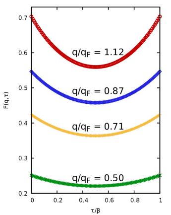
Figure 3: Ab initio PIMC results for the imaginary-time density–density correlation function $F(q,\tau)$ for fixed wave numbers at $r_{s}=4$, $\theta=2$, and $N=66$.

In Fig. 3, we show results for the $\tau$-dependence of this quantity for $N=66$ unpolarized electrons at $r_{s}=4$ and $\theta=2$ for four different wave numbers $q=|\mathbf{q}|$ in the vicinity of the Fermi wave number $q_{\textnormal{F}}$. First and foremost, we note that $F$ is always symmetric with respect to $\tau=\beta/2$, i.e., $F(\mathbf{q},\tau)=F(\mathbf{q},\beta-\tau)$ (for $\tau\leq\beta/2$). In addition, the magnitude of $F$ increases monotonically with increasing $q$ in the depicted regime of wave vectors. This can be understood by recalling its relation to the static structure factor, $F(\mathbf{q},\tau=0)=S(\mathbf{q})$, with $S(\mathbf{q})$ following a parabola for small $q$ and being monotonically increasing up to around thrice the Fermi wave number, see Fig. 7 for a graphical depiction and Refs. dornheim_prl ; dornheim_cpp ; review for an extensive discussion. Lastly, we mention that the slope of $F$ becomes increasingly steep for larger $q$; a trend that persists for even larger wave numbers as can be seen in Fig. 4 where we show PIMC results for up to $q/q_{\textnormal{F}}\approx 6$.

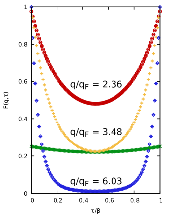
Figure 4: Same as Fig. 3, but for larger wave numbers. The green curve is shown as a reference and corresponds to $q/q_{\textnormal{F}}=0.50$, i.e., to the green curve in Fig. 3.

In particular, $F(\mathbf{q},\tau)$ almost decays to zero around $\tau=\beta/2$ for large $q$.

Let us next study the impact of Coulomb coupling effects by considering different values of the density parameter $r_{s}$. In Fig. 5, we compare our results for $F(\mathbf{q},\tau)$ again for $N=66$ unpolarized electrons at $\theta=2$ for $r_{s}=4$ (solid red), $r_{s}=6$ (dash-dotted black), and $r_{s}=20$ (dashed green). The wave number has been chosen as $q/q_{\textnormal{F}}\approx 2$ corresponding to the physically most interesting regime where the dispersion relation of $S(\mathbf{q},\omega)$ is actually negative for strong coupling, like in the case of $r_{s}=20$, see Fig. 17.

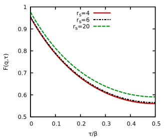
Figure 5: Imaginary-time density–density correlation function $F(q=2q_{\textnormal{F}},\tau)$ at $\theta=2$ and $N=66$ for $r_{s}=4$ (solid red), $r_{s}=6$ (dash-dotted black), and $r_{s}=20$ (dashed green).

Indeed, while the curves for $r_{s}=4$ and $r_{s}=6$ are nearly identical, the $r_{s}=20$ results significantly differ both in magnitude and slope, cf. the corresponding dynamic structure factors $S(\mathbf{q},\omega)$ shown in Fig. 17.

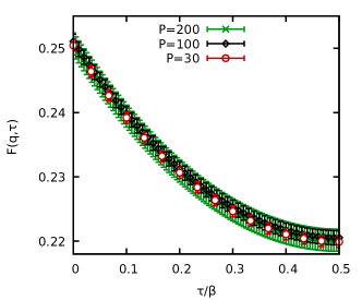
Figure 6: Imaginary-time density–density correlation function $F(q=0.5q_{\textnormal{F}},\tau)$ at $\theta=2$, $r_{s}=4$, and $N=66$ for different numbers of imaginary-time propagators $P$.

For completeness, let us also consider the dependence of the imaginary-time density correlation function on the number of propagators $P$. This is investigated in Fig. 6, where we show results for $F$ for $N=66$ electrons at $r_{s}=4$ and $\theta=2$ for $q/q_{\textnormal{F}}\approx 0.5$. The different symbols correspond to PIMC data for $P=30$ (red circles), $P=100$ (black diamonds), and $P=200$ (green crosses, in the background). Evidently, the four different data sets cannot be distinguished within the statistical uncertainty and the only difference is given by the different $\tau$-grid. The situation somewhat changes towards lower temperatures and larger $q$, and the convergence with $P$ was carefully checked for all considered cases throughout this work.

Let us conclude our consideration of $F(\mathbf{q},\tau)$ with a depiction of this quantity over the entire relevant $\tau$-$q$-plane.

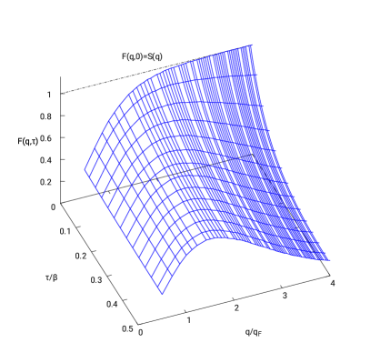
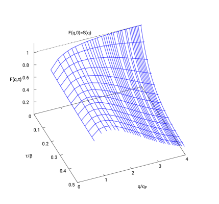
Figure 7: Imaginary-time density–density correlation function $F(q,\tau)$ for $\theta=2$ and $r_{s}=4$, $N=66$ (top) and $r_{s}=1$, $N=34$ (bottom). $F(q,\tau)$ is symmetric with respect to $\tau=\beta/2$ and becomes equivalent to the static structure factor $S(q)$ for $\tau=0$.

This is shown for $N=66$, $\theta=2$, and $r_{s}=4$ in the top panel of Fig. 7. Since a physically meaningful interpretation of this quantity is rather difficult, we restrict ourselves to mentioning that $F$ converges to the static structure factor for $\tau=0$ and exhibits a distinct structure around $q=2q_{\textnormal{F}}$. The bottom panel of the same figure corresponds to $N=34$, $\theta=2$, and $r_{s}=1$. At this higher density, correlation effects are less important and the structure in $F(\mathbf{q},\tau)$ becomes less pronounced.

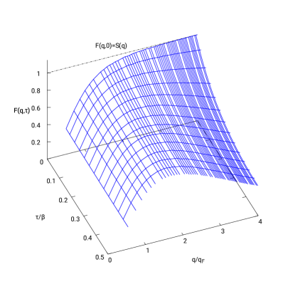
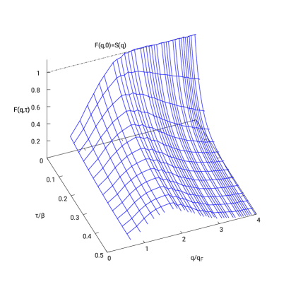
Figure 8: Imaginary-time density–density correlation function $F(q,\tau)$ for $r_{s}=6$ and $\theta=4$, $N=66$ (top) and $\theta=0.75$, $N=34$ (bottom).

Lastly, we show PIMC results for $F$ for $r_{s}=6$ and $\theta=4$ (Fig. 8, top) and $\theta=0.75$ (bottom). Again, we observe that the larger impact of correlation effects leads to a significantly more structured imaginary-time correlation function at the lower temperature. The somewhat noisy progression in the case of $\theta=0.75$ around $q=2q_{\textnormal{F}}$ is a result of the increased statistical uncertainty in our PIMC data due to the fermion sign problem with an average sign of $S\approx 0.023$.

III.2 Static density-response function and local field corrections

Another important quantity that is of considerable interest in its own right is the static density–density response function $\chi(\mathbf{q})$, which is obtained from $F(\mathbf{q},\tau)$ via a simple one-dimensional integration along the $\tau$-axis, see Eq. (19).

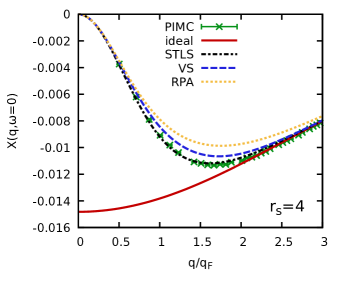
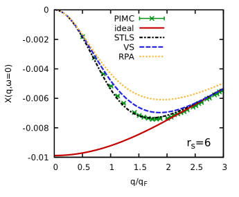
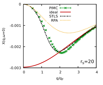
Figure 9: Wave number dependence of the static response function $\chi(q,\omega=0)$ [in Hartree atomic units] at $\theta=2$ for $r_{s}=4$ (top), $r_{s}=6$ (center), and $r_{s}=20$ (bottom). Shown are PIMC data for $N=66$ (green crosses), the ideal function $\chi_{0}(q,\omega=0)$ (solid red), STLS stls ; stls2 (dash-dotted black), VS stls2 (dashed blue), and RPA (dotted yellow).

In Fig. 9, we show results for the wave number dependence of $\chi(\mathbf{q})$ for $N=66$ unpolarized electrons at $\theta=2$ for three different coupling strengths. The green crosses depict our PIMC data with the corresponding statistical uncertainty, which is of the order of $\Delta\chi/\chi\sim 10^{-3}$ at these parameters. We stress that the evaluation of Eq. (19) allows to evaluate the entire $\mathbf{q}$-dependence of $\chi$ from a single PIMC simulation, which is in stark contrast to the recently proposed simulation of a harmonically perturbed system dornheim_pre ; groth_jcp . In the latter case, one has to perform multiple full QMC simulations of an inhomogeneous system governed by Eq. (6) for several values of the perturbation amplitude $A$ to obtain $\chi(\mathbf{q})$ for a single wave number. Hence, that strategy is only advisable when $F(\mathbf{q},\tau)$ is not accessible, which is the case for the novel permutation blocking PIMC and configuration PIMC methods that are available over more significant parts of the WDM regime beyond standard PIMC. To summarize, the PIMC evaluation of Eq. (19) constitutes the method of choice wherever possible, and allows to obtain a bulk of accurate data over the entire $q$-range. However, when PIMC breaks down due to the fermion sign problem, the application of PB-PIMC and CPIMC is a valuable alternative of a complementary nature to obtain accurate data for $\chi(\mathbf{q})$ and $G(\mathbf{q})$ in the WDM regime, where quantum degeneracy effects are even more important.

In the top panel of Fig. 9, we compare the PIMC results for $r_{s}=4$ to the ideal density-response function $\chi_{0}(\mathbf{q})$ (solid red line) and various other theories, see Ref. review for an extensive recent review article. First and foremost, we note that all data sets (except the ideal curve) exhibit the correct parabolic behavior kugler2 ,

$$\lim_{q\to 0}\chi(\mathbf{q})=-\frac{q^{2}}{4\pi}\quad,$$ (35)

for small wave numbers, which is a direct consequence of perfect screening in the UEG. The dotted yellow line corresponds to the RPA, which entails a mean-field description of the response to an external perturbation. Thus, the RPA is accurate at high density and temperature, but exhibits only a qualitative agreement with the exact PIMC data even for $r_{s}=4$, with the systematic deviations being most pronounced for intermediate wave numbers $0.5q_{\textnormal{F}}\lesssim q\lesssim 3q_{\textnormal{F}}$. The dashed blue curve has been obtained using the approximate static local field correction $G_{\textnormal{VS}}(\mathbf{q})$ from the Vashishta-Singwi (VS) formalism vs_original ; stolzmann taken from Sjostrom and Dufty stls2 (see Fig. 10 for the actual corresponding $G(\mathbf{q})$ data). Evidently, the incorporation of $G_{\textnormal{VS}}$ leads to a significant improvement over the RPA for all $q$-values, although it remains inaccurate most notably around $q=1.5q_{\textnormal{F}}$. Lastly, the dash-dotted black line corresponds to the approximate static local field correction $G_{\textnormal{STLS}}(\mathbf{q})$ proposed by Singwi, Tosi, Land, and Sjölander (STLS) stls_original for the ground-state, which was extended in Refs. stls ; stls2 ; tanaka_new to the WDM regime. The STLS formalism proves to be significantly more accurate than both RPA and VS, which is in agreement with previous findings for the static structure factor $S(\mathbf{q})$ and the interaction energy $v$ discussed in Refs. review ; dornheim_cpp ; groth_prl ; dornheim_pop .

Upon increasing the coupling strength to $r_{s}=6$ (center) and $r_{s}=20$ (bottom), all depicted approximations become noticeably less accurate, although STLS still looks impressive in the former case. However, at strong coupling, even $G_{\textnormal{STLS}}(\mathbf{q})$ cannot capture the effect of XC contributions and the corresponding $\chi_{\textnormal{STLS}}(\mathbf{q})$ exhibits both a wrong peak position and magnitude. Nevertheless, the complete negligence of $G$ in the case of RPA leads to systematic deviations of the order of $100\%$.

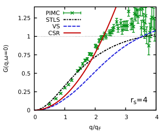
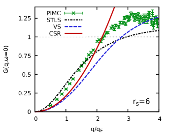
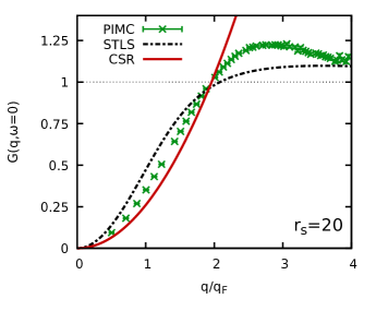
Figure 10: Wave number dependence of the static local field correction $G(q,\omega=0)$ at $\theta=2$ for $r_{s}=4$ (top), $r_{s}=6$ (center), and $r_{s}=20$ (bottom). Shown are PIMC data for $N=66$ and $P=100$ (green crosses), STLS stls ; stls2 (dash-dotted black), VS stls2 (dashed blue), and the compressibility sum-rule (CSR, solid red), cf. Eq. (36).

Let us next discuss the static local field correction $G(\mathbf{q})$, which is shown in Fig. 10 for the same conditions as $\chi(\mathbf{q})$ in Fig. 9. Recall that the RPA corresponds to setting $G_{\textnormal{RPA}}(\mathbf{q})=0$. In addition, the solid red curve corresponds to the exact limit for small wave numbers that directly follows from the compressibility sum-rule (CSR) stls2 ; review

$$\lim_{q\to 0}G(\mathbf{q})=-\frac{q^{2}}{4\pi}\frac{\partial}{\partial n^{2}}\left(nf_{\textnormal{xc}}\right)\quad,$$ (36)

with $n$ being the total electronic density. In practice, Eq. (36) is evaluated using the accurate parametrization of the XC-free energy from Ref. groth_prl . Evidently, the CSR-curves do not overlap with our PIMC data (green crosses), as the small-$q$ limit is not accessible due to the finite simulation box, see Refs. dornheim_prl ; review for an analog discussion of the static structure factor $S(\mathbf{q})$. Furthermore, it is well-known that the STLS curve (dash-dotted black) violates the CSR, even if we replace the exact $f_{\textnormal{xc}}$ in Eq. (36) by the corresponding STLS expression $f^{\textnormal{STLS}}_{\textnormal{xc}}$, see, e.g., Ref. stls2 . In contrast, the VS-curve is in good agreement with the CSR, which is an understandable, yet nontrivial finding: while the expression for the static local field correction $G_{\textnormal{VS}}(\mathbf{q})$ is derived by imposing the CSR, this is done by assuming the approximate expression for $f_{\text{xc}}$ within the VS formalism, $f_{\textnormal{xc}}^{\textnormal{VS}}$, which is known to be even less accurate than, for example, $f_{\textnormal{xc}}^{\textnormal{STLS}}$. Still, this condition leads to an accurate static local field correction for small $q$.

For larger wave numbers, we observe an increased statistical uncertainty, which is a direct consequence of the evaluation of Eq. (19): within a PIMC simulation, we obtain data for $F(\mathbf{q},\tau)$, which, in turn, is used to compute the static density-response function $\chi(\mathbf{q})$ via Eq. (10). The static local field correction is then obtained by measuring the deviation of $\chi$ to the noninteracting case, cf. Eq. (28). For large wave numbers $q$, the effect of $G(\mathbf{q})$ on the total response function $\chi$ is suppressed by the $4\pi/q^{2}$ pre-factor in Eq. (24) and $\chi$ eventually converges towards the ideal function $\chi_{0}(\mathbf{q})$, see Fig. 9. Therefore, $G$ becomes the relatively small difference between two large numbers in this regime, and the relative uncertainty in this quantity increases. Still, we stress that the quality of the present QMC data for $G(\mathbf{q})$ is significantly better than analog results from simulations of the harmonically perturbed system both at finite temperature dornheim_pre ; groth_jcp and in the ground state moroni2 ; bowen2 .

Despite the relatively high accuracy of the VS and, in particular, the STLS scheme in the description of $\chi(\mathbf{q})$ at $r_{s}=4$ and $r_{s}=6$, see Fig. 9, these approximations perform significantly worse for $G(\mathbf{q})$ itself. This is not surprising, as the static local field correction provides a wave-number resolved description of exchange-correlation effects and, therefore, is even more sensitive to an approximate treatment of the Coulomb repulsion than $f_{\textnormal{xc}}$. Furthermore, both VS and STLS are static theories, which means that they completely neglect the frequency-dependence of $G(\mathbf{q},\omega)$. Naturally, this shortcoming affects the static limit of this quantity, which, in turn means that such theories cannot be systematically improved to provide exact results for $G(\mathbf{q})$. In contrast, while our PIMC simulations, too, only yield results for the static limit of $G$, the frequency-dependence of XC-effects is fully included in the imaginary-time formulation of the approach and the corresponding PIMC results are exact.

Finally, in the bottom panel of Fig. 10 we show results for $G$ for strong coupling, $r_{s}=20$. In this case, the STLS scheme can only provide a qualitative description and the maximum in $G$ around $q=2.5q_{\textnormal{F}}$ is not captured at all.

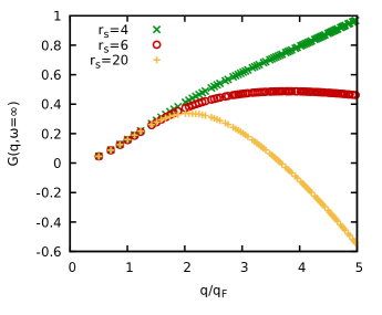
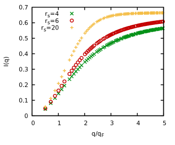
Figure 11: Wave number dependence of the high-frequency limit of the dynamic local field correction $G(q,\omega=\infty)$ (top) and interaction integral $I(q)$ (bottom, Hartree atomic units) at $\theta=2$ and $N=66$ for $r_{s}=4$ (green crosses), $r_{s}=6$ (red circles), and $r_{s}=20$ (yellow pluses).

Lastly, let us consider the high-frequency limit of the local field correction, which is obtained from our PIMC data for $S(\mathbf{q})$ and the kinetic energy $K$ via Eq. (29).

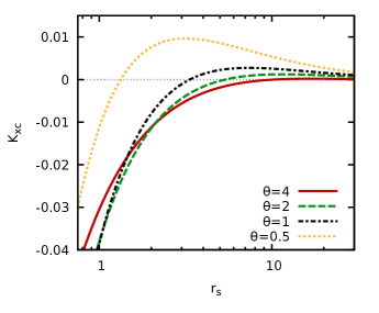
Figure 12: Density dependence of the exchange–correlation contribution to the kinetic energy $K_{\textnormal{xc}}$ [in Hartree atomic units] for $\theta=4$ (solid red), $\theta=2$ (dashed green), $\theta=1$ (dash-dotted black), and $\theta=0.5$ (dotted yellow). Computed from the accurate parametrization of $f_{\textnormal{xc}}$ from Ref. groth_prl .

In the top panel of Fig. 11, we show results for the wave number dependence of $G(\mathbf{q},\omega=\infty)$ for the same conditions as in Fig. 10. Evidently, the three data sets for $r_{s}=4$ (green crosses), $r_{s}=6$ (red circles), and $r_{s}=20$ (yellow pluses) exhibit a quite distinct behavior: while all curves are in good agreement for small $q$, the $r_{s}=4$ results for $G(\mathbf{q},\omega=\infty)$ continue to increase for large $q$, whereas both the $r_{s}=6$ curve and, to an even more significant degree, the $r_{s}=20$ curve decrease in this regime. In fact, the yellow curve attains negative values for $q\gtrsim 3q_{\textnormal{F}}$. This finding can be understood by considering the two contributions to $G(\mathbf{q},\omega=\infty)$, i.e., the interaction integral $I(q)$ [see Eq. (4)] and a parabola with a pre-factor proportional to the negative XC-part to the kinetic energy $-K_{\textnormal{xc}}$ [see Eq. (4)]. For small wave numbers, $I(q)$ dominates as can be seen in the bottom panel of Fig. 11 and is monotonically increasing with $q$. Eventually, however, the parabolic term takes over, and the particular behavior of $G(\mathbf{q},\omega=\infty)$ is determined by $K_{\textnormal{xc}}$, which is plotted in Fig. 12.

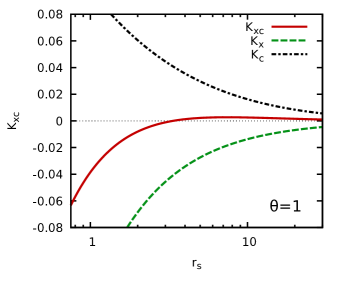
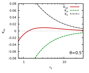
Figure 13: Shown is the density dependence of the exchange–correlation kinetic energy $K_{\textnormal{xc}}$ [in Hartree atomic units], and the separate contributions $K_{\textnormal{x}}$ and $K_{\textnormal{c}}$, for $\theta=1$ (top) and $\theta=0.5$ (bottom). Computed from the accurate parametrization of $f_{\textnormal{xc}}$ from Ref. groth_prl and of $f_{\textnormal{x}}$ from Ref. F .

For the highest depicted reduced temperature, $\theta=4$ (solid red), $K_{\textnormal{xc}}$ is negative for $r_{s}\lesssim 10$. In contrast, for $\theta=0.5$ (dotted yellow) this is the case for $r_{s}\lesssim 1$. With these findings, the observed large-$q$ behavior in the top panel of Fig. 11 becomes obvious: negative values of $K_{\text{xc}}$, as in the case of $\theta=2$ and $r_{s}=4$, lead to positive pre-factors of the parabola and $G(\mathbf{q},\omega=\infty)$ remains strictly increasing; positive values of $K_{\textnormal{xc}}$, on the other hand, result in a negative parabola as observed for $r_{s}=6$ and $r_{s}=20$. For completeness, we note that similar findings have been observed for the ground state in Ref. iwamoto .

Let us conclude this section by investigating the origin of the nontrivial progression of $K_{\textnormal{xc}}$. To this end, we plot the individual exchange and correlation parts, $K_{\textnormal{x}}$ (dashed green) and $K_{\textnormal{c}}$ (dash-dotted black), to $K_{\textnormal{xc}}$ (solid red) in Fig. 13. Note that $K_{\textnormal{x}}$ is obtained by replacing $f_{\textnormal{xc}}$ in Eq. (4) with the noninteracing free energy $f_{\textnormal{x}}$, which was parametrized by Perrot and Dharma-wardana F . Interestingly, $K_{\textnormal{xc}}$ is given by the relatively small difference of the positive exchange and the negative correlation parts. More specifically, the correlation contribution dominates for low temperatures and large values of the coupling parameter $r_{s}$, and $K_{\textnormal{xc}}$ attains positive values. Evidently, this happens for even smaller $r_{s}$-values at the lower temperature, $\theta=0.5$ (bottom panel).

III.3 Stochastic sampling method

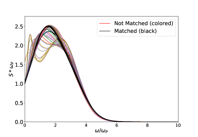
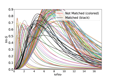
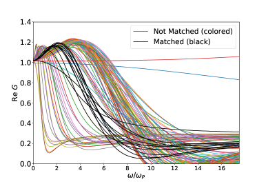
Figure 14: Reconstruction of the dynamic structure factor $S(|\mathbf{q}|\approx 1.98q_{\textnormal{F}},\omega)$ for $N=34$ unpolarized electrons at $r_{s}=6$ and $\theta=1$. The top panel shows a set of $M=115$ trial solution $S_{\textnormal{trial},i}$, with the black (coloured) curves having (not) been included into the final average, Eq. (33). The central and bottom panels depict the corresponding trial functions for the imaginary and real parts of the dynamic local field correction, see Sec. II.5 for an extensive theoretical introduction.

In the following section, we give a hands-on discussion of two examples of our stochastic sampling scheme (see Sec. II.5) to compute the dynamic structure factor $S(\mathbf{q},\omega)$ from our PIMC data. See Sec. III.4, for a discussion of our findings for this quantity for different densities and temperatures.

In Fig. 14, we show trial solutions for $S(\mathbf{q},\omega)$ (top), $\textnormal{Im}G(\mathbf{q},\omega)$ (center), and $\textnormal{Re}G(\mathbf{q},\omega)$ (bottom) that have been generated by following the procedure from Sec. II.5 for $N=34$ electrons at $r_{s}=6$ and $\theta=1$ around twice the Fermi wave vector. In particular, the black curves are valid solutions that are included in the final average $S_{\textnormal{final}}(\mathbf{q},\omega)$ [Eq. (33)], whereas the coloured curves violate the corresponding imaginary-time correlation–function $F(\mathbf{q},\tau)$ and the frequency moments $\braket{\omega^{k}}$. Upon examining the dynamic structure factor, we find that the stochastic sampling of $G(\mathbf{q},\omega)$ leads to (at least) two distinct classes of trial solution for $S$. More specifically, there appear $S_{\textnormal{trial}}(\mathbf{q},\omega)$ with a pronounced double-peak structure (which do not fulfill the PIMC boundary conditions), with the first one sometimes being interpreted as a diffusive peak jan1 . In addition, there are solutions with a single broad peak around $\omega=2\omega_{\textnormal{p}}$, which provide those $S$ that fulfill all known requirements from our PIMC simulations. Interestingly, though, slight variations in the form and/or position of the peak lead to a significant disagreement regarding $F(\mathbf{q},\tau)$ and $\braket{\omega^{k}}$, and the corresponding $S_{\textnormal{trial}}$ are, consequently, discarded. This is in stark contrast to the $\theta=2$ case, which is show in Fig. 15 and discussed below.

The central panel of Fig. 14 shows the corresponding stochastically sampled imaginary parts of the dynamic local field correction, cf. Eq. (31). All depicted curves exhibit a fairly similar progression with the exact conditions $\textnormal{Im}G(\mathbf{q},0)=\textnormal{Im}G(\mathbf{q},\infty)=0$ and a single peak in between. However, the peak position, width, and high-frequency tail are significantly different from each other. Moreover, the bottom panel shows the real part of $G(\mathbf{q},\omega)$, which has been obtained from $\textnormal{Im}G(\mathbf{q},\omega)$ via the Kramers-Kronig relation Eq. (25) by numerical integration. Interestingly, this procedure leads to a more complicated functional form: starting from the exact static limit for $\omega\to 0$, $\textnormal{Re}G(\mathbf{q},\omega)$ always exhibits a monotonic increase for small $\omega$, followed by a maximum, which varies drastically in its position depending on the chosen trial parameters $a_{i}$, $b_{i}$, and $c$. Moreover, there appears a minimum for intermediate frequencies, until the exact high-frequency limit is reached from below. Again, the particular form of this tail can be very different.

While the mapping from $G_{\textnormal{trial}}(\mathbf{q},\omega)$ onto $S_{\textnormal{trial}}(\mathbf{q},\omega)$ is far from obvious, we find that those $\textnormal{Im}G(\mathbf{q},\omega)$ with a maximum at low frequency result in a double-peaked dynamic structure factor with the aforementioned diffusive feature. In addition, we note that fairly different trial solutions both in the imaginary and real parts of the dynamic local field correction lead to very similar results in $S_{\textnormal{trial}}(\mathbf{q},\omega)$ itself. Since our PIMC data for $F(\mathbf{q},\tau)$ and $\braket{\omega^{k}}$ only allow us to decide between differences in the dynamic structure factor itself, it follows that $G(\mathbf{q},\omega)$ is much less restrained by our reconstruction procedure than $S(\mathbf{q},\omega)$.

As a side remark, we mention that the parametrization of $\textnormal{Im}G(\mathbf{q},\omega)$ from Eq. (31) has proven sufficiently flexible even at strong coupling ($r_{s}=10,20$), when a nontrivial incipient excitonic feature emerges. Still, it can potentially be systematically improved by including higher powers in $\omega$, which will likely be necessary for even stronger coupling, which, however, is beyond the scope of the present work. Further, we mention that only $7$ of the $M=115$ trial solution shown in Fig. 14 are actually included into the computation of the final result, and the distribution of the $\textnormal{Re}G$ and $\textnormal{Im}G$ curves is far from uniform. This leaves open the possibility to further improve our sampling procedure in future work. Moreover, the parametrization of $\textnormal{Im}G$ and subsequent calculation of $\textnormal{Re}G$ (cf. Sec. II.5) that is employed in this work is not the only choice, and other interpolations between the known limits of $G(\mathbf{q},\omega)$ have been reported elsewhere jan1 ; hong1 ; hong2 .

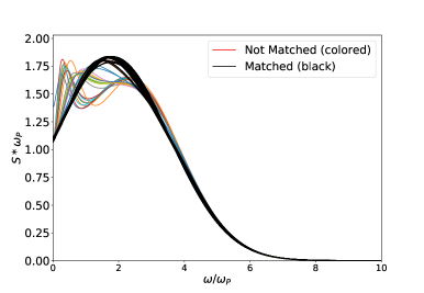
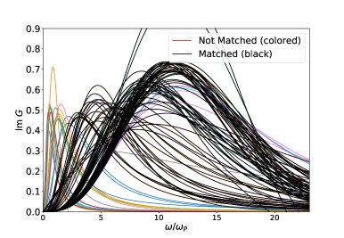
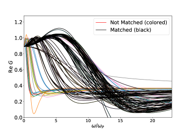
Figure 15: Reconstruction of the dynamic structure factor $S(|\mathbf{q}|\approx 1.98q_{\textnormal{F}},\omega)$ for $N=34$ unpolarized electrons at $r_{s}=6$ and $\theta=2$. The top panel shows a set of $M=99$ trial solution $S_{\textnormal{trial},i}$, with the black (coloured) curves having (not) been included into the final average, Eq. (33). The central and bottom panels depict the corresponding trial functions for the imaginary and real parts of the dynamic local field correction, see Sec. II.5 for an extensive theoretical introduction.

Let us conclude this discussion of the stochastic sampling reconstruction procedure by increasing the temperature to $\theta=2$, which is shown in Fig. 15. Remarkably, in this case we find a significantly increased ratio of included (black) to discarded (coloured) solutions. More specifically, the appearing double-peak structure factors are still not in agreement with our PIMC data for $F(\mathbf{q},\tau)$ and $\braket{\omega^{k}}$, whereas nearly all solutions from the class with only a single broad peak are included into the construction of the final average $S_{\textnormal{final}}(\mathbf{q},\omega)$. Upon examining the corresponding dynamic local field corrections, we find that almost only those $\textnormal{Im}G(\mathbf{q},\omega)$ are discarded that have a maximum at very low-frequency. Consequently, $G(\mathbf{q},\omega)$ is even less determined by our PIMC data for the higher temperature than for $\theta=1$, as the impact on observable quantities is smaller. Still, the dynamic structure factor itself remains of high quality.

III.4 Dynamic structure factors

Let us conclude this paper with a presentation of new results for the dynamic structure factor $S(\mathbf{q},\omega)$ for different densities and temperatures.

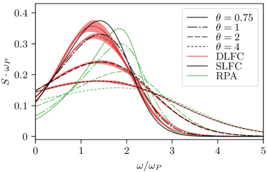
Figure 16: Dynamic structure factor $S(q\approx 1.4q_{\textnormal{F}},\omega)$ of the warm dense electron gas with $N=34$ and $r_{s}=6$ for different temperatures. The solid red, dashed black, and solid green lines depict data from our stochastically sampled dynamic local field correction, the static approximation $G_{\textnormal{static}}(\mathbf{q},\omega)=\textnormal{Re}G(\mathbf{q},0)$, and the random phase approximation (RPA), respectively.

In Fig. 16, we show the dynamic structure factor $S(\mathbf{q},\omega)$ for an intermediate wave number $q/q_{\textnormal{F}}\approx 1.4$ for $N=34$ unpolarized electrons at a metallic density, $r_{s}=6$, for four different temperatures. Note that the line type (i.e., solid, dashed, etc.) distinguishes $\theta$, while the different colors correspond to different methods. More specifically, the green curves depict the random phase approximation (RPA), where exchange-correlation effects on the density-response are completely neglected, i.e., $G_{\textnormal{RPA}}(\mathbf{q},\omega)=0$. Furthermore, the black curves have been obtained using the so-called static approximation, where the exchange-correlation effects are treated statically, $G_{\textnormal{static}}(\mathbf{q},\omega)=\textnormal{Re}G(\mathbf{q},0)$. For completeness, we note that here we use the exact static limit obtained from our PIMC simulations, Eq. (28), which is in contrast to static dielectric theories like STLS or VS, cf. Sec. III.2. Lastly, the red coloured curves correspond to the exact solutions that have been computed using our new stochastic sampling reconstruction method for the dynamic local field correction, which has been introduced in detail in the previous section. In addition, the shaded red area depicts the corresponding degree of uncertainty, which is estimated as the variance of all accepted trial solutions $S_{\textnormal{trial}}(\mathbf{q},\omega)$, Eq. (34).

At the largest considered temperature, $\theta=4$ (dotted curves), the influence of the LCF is relatively weak. Consequently, the uncertainty interval in the exact solution is relatively small. Furthermore, quantum effects do not dominate the dynamic density response, and the static approximation is in exact agreement with the DLFC curve over the entire $\omega$-range. In contrast, the RPA curve only qualitatively reproduces the other two data sets even at these relatively weakly coupled parameters.

Upon decreasing the temperature, the system simultaneously becomes more strongly coupled and more quantum mechanical. The first fact leads to severe systematic errors in the RPA, which significantly overestimates the peak position and underestimates the height. On the other hand, the quantum nature of the dynamic density response cannot be fully captured by a static local field correction, and the accuracy of the black curves declines with decreasing $\theta$. Still, we stress that the SLFC constitutes a substantial improvement over the RPA everywhere, and the observed disagreements are quantitative, but not qualitative. Moreover, the impact of the frequency dependence of $G(\mathbf{q},\omega)$ is even less severe than in the previously investigated example of $r_{s}=10$, see Ref. dornheim_dynamic .

Figure 17: Dispersion relation of the dynamic structure factor $S(\mathbf{q},\omega)$ of the warm dense electron gas with $N=66$ and $\theta=2$ for $r_{s}=4$ (left), $r_{s}=6$ (center), and $r_{s}=20$ (right). The solid red, dashed black, and solid green lines depict data from our stochastically sampled dynamic local field correction, the static approximation $G_{\textnormal{static}}(\mathbf{q},\omega)=\textnormal{Re}G(\mathbf{q},0)$, and the random phase approximation (RPA), respectively. The curves have been re-scaled for a better comparability.

Finally, we show entire dispersion relations of the dynamic structure factor for $N=66$ unpolarized electrons at $\theta=2$ for $r_{s}=4$, $r_{s}=6$, and $r_{s}=20$ in Fig. 17.

First and foremost, we find that both at $r_{s}=4$ and $r_{s}=6$, which correspond to metallic densities falling well into the warm dense matter regime, the static approximation cannot be distinguished from the exact solution over the entire range of wave numbers $q$. In contrast, the RPA again only exhibits a qualitative agreement and is fairly inaccurate both regarding peak position and width for intermediate wave numbers, $q/q_{\textnormal{F}}\sim 2$. At $r_{s}=20$, which is a strongly coupled system more closely resembling an electron liquid, the total negligence of exchange-correlation effects renders the RPA completely inappropriate. The static approximation, on the other hand, constitutes a spectacular improvement and almost exactly reproduces the exact solutions found via our stochastic sampling scheme. In particular, the incipient excitonic feature, which manifests as a pronounced red-shift at intermediate wave numbers, is fully captured by the black curves dornheim_dynamic .

Therefore, we conclude that the static approximation [using our exact PIMC data for $G(q)$] does indeed provide a reliable and readily available tool to accurately compute the dynamic structure factor $S(\mathbf{q},\omega)$. This is particularly important at even lower temperatures and higher densities, where the present combination of PIMC and the stochastic sampling of the DLFC is prevented by the fermion sign problem, but $G_{\textnormal{static}}$ is accessible via the more advanced PB-PIMC and CPIMC methods dornheim_pre ; groth_jcp .

IV Summary and discussion

In this work, we have presented an ab initio path integral Monte Carlo study of the density-response of the uniform electron gas at extreme temperature and density.

First of all, we have introduced in detail the underlying theory, in particular the concept of the imaginary-time correlation-function $F(\mathbf{q},\tau)$, and its connection to the desired response functions. In particular, our new extensive PIMC data for $F$ have allowed us to present exact data for the static density-response function $\chi(\mathbf{q})$ and the corresponding static local field correction $G(\mathbf{q})$ from warm dense matter to the strongly correlated electron liquid regime. A comparison of these data to standard dielectric theories has revealed the following: (a) the random phase approximation reveals significant inaccuracies even at $r_{s}=4$ and $\theta=2$ and fully breaks down at $r_{s}=20$; (b) the approximate static local field correction by Vashista-Singwi leads to a significantly improved description of $\chi(\mathbf{q})$, and $G_{\textnormal{VS}}(\mathbf{q})$ is highly accurate at small $q$, which is due to the incorporation of the compressibility sum-rule. However, for larger wave numbers, the static LFC exhibits significant systematic deviations; (c) the static LFC due to Singwi-Tosi-Land-Sjölander constitutes the most accurate dielectric method both for $\chi$ and $G$, although at strong coupling ($r_{s}=20$) it, too, is only capable to provide a qualitative description of the static density-response. In this context, a future comparison of our exact PIMC data to the new hypernetted-chain (HNC) based static LFC by Tanaka tanaka_hnc and the quantum STLS (qSTLS) method schweng ; arora might be valuable to evaluate the source of the errors in the dielectric methods: if the HNC approach would constitute a significant improvement at large $r_{s}$, the error in the STLS and VS schemes would be the approximate treatment of exchange-correlation effects in the static local field correction; a superior performance of qSTLS, on the other hand, would indicate the importance of the frequency dependence of $G(\mathbf{q},\omega)$, which is neglected in STLS, VS, and HNC, but consistently included in qSTLS.

Secondly, our study of the high-frequency limit of $G(\mathbf{q},\omega)$ at twice the Fermi temperature has revealed different behaviours at large wave numbers depending on the coupling parameter $r_{s}$: for small $r_{s}$, $G(\mathbf{q},\omega=\infty)$ increases with $q$, whereas the opposite holds at strong coupling (even at $r_{s}=6$) and $G(\mathbf{q},\omega=\infty)$ actually attains negative values. This is consistent with previous findings at zero temperature iwamoto and was explained by a nontrivial behaviour of the exchange–correlation part of the kinetic energy, $K_{\textnormal{XC}}$, shown in Fig. 12.

Thirdly, we have given both an extensive introduction to the theoretical aspects and a practical demonstration of our new reconstruction method that allows us to obtain highly accurate results for the dynamic structure factor $S(\mathbf{q},\omega)$ purely on the basis of our PIMC data for the thermodynamic equilibrium, see Sec. III.3. While the basic idea and first results for $S(\mathbf{q},\omega)$ were already shown in Ref. dornheim_dynamic , here we provide an explicit demonstration of the stochastic sampling of the dynamic LFC, and how this leads to trial solutions $S_{\textnormal{trial}}(\mathbf{q},\omega)$, which are subsequently compared to our PIMC data for $F(\mathbf{q},\tau)$ and $\braket{\omega^{k}}$. We are confident that this comprehensive discussion will render our findings replicable and make the future adaption of our scheme to related problems in other fields possible. In addition, the most significant new finding is the comparably high quality in the final results for the dynamic structure factor, which is in stark contrast to the real and imaginary parts of $G(\mathbf{q},\omega)$. More specifically, quite different trial solutions for $G_{\textnormal{trial},i}(\mathbf{q},\omega)$ lead to nearly identical $S_{\textnormal{trial},i}(\mathbf{q},\omega)$ and, therefore, cannot be selected or discarded on the basis of $F$ and $\braket{\omega^{k}}$, which explicitly depend on the dynamic structure factor, only.

In the fourth place, we have shown extensive new data for the dynamic structure factor of the UEG for hitherto unexplored parameters. Fully in accord with Ref. dornheim_dynamic , we find significant systematic errors in the random phase approximation even at relatively weak coupling, which are most pronounced around twice the Fermi wave number $q_{\textnormal{F}}$. In contrast, the static approximation, i.e., using the exact static limit of $G$ for all frequencies, leads to nearly exact results for even for the electron liquid at $r_{s}=20$. Furthermore, it retains an impressive accuracy with decreasing temperature and, in a nutshell, allows for a good description of $S(\mathbf{q},\omega)$ for all investigated parameters.

Let us conclude this paper by outlining a number of interesting topics for future research.

Accurate data for $S(\mathbf{q},\omega)$ of the warm dense UEG are important for the interpretation of experiments within the widespread Chihara decomposition chihara1 ; chihara2 . To this end, a readily available parametrization of the static local field correction $G(\mathbf{q};r_{s},\theta)$ connecting the ground state results cdop ; farid with PIMC results at finite temperature constitutes a highly desirable goal. Further, the PIMC data for the LFC could be complemented by configuration PIMC groth_jcp and permutation blocking PIMC data dornheim_pre at stronger quantum degeneracy (i.e., low temperature and high density), where our present strategy fails due to the fermion sign problem.

Our new data for $S(\mathbf{q},\omega)$ can also be used to benchmark approximate methods for the description of quantum dynamics at finite temperature, such as nonequilibrium Green functions kas1 ; kas2 ; kas3 ; kwong and the method of moments by Tkachenko and co-workers igor1 ; igor2 ; igor_quantum .

Moreover, the observed negative dispersion relation in $S(\mathbf{q},\omega)$ (see also Ref. dornheim_dynamic ) constitutes an interesting feature in its own right. While the interpretation as an incipient excitonic feature from Refs. takada1 ; takada2 ; higuchi is plausible, its manifestation in the warm dense UEG deserves a more detailed investigation. For completeness, we mention that a similar behaviour has been observed in the classical one-component plasma ott , and in experiments with alkali metals vomFelde .

Finally, the stochastic sampling method for the reconstruction of a dynamic quantity is, in principle, not limited to the present application to PIMC data for the UEG. For example, while the computation of imaginary-time correlation-functions in ground state QMC simulations wmc_review of fermions is nontrivial motta1 , Motta et al. motta2 recently obtained accurate results for $F(\mathbf{q},\tau)$ for a $2D$ UEG at zero temperature using a phaseless auxiliary field QMC approach.

References

References

- (1) G. Giuliani and G. Vignale, Quantum Theory of the Electron Liquid, Cambridge University Press (2008)
- (2) P.-F. Loos and P.M.W. Gill, The uniform electron gas, Comput. Mol. Sci. 6, 410-429 (2016)
- (3) S.H. Vosko, L. Wilk, and M. Nusair, Accurate Spin-Dependent Electron Liquid Correlation Energies for Local Spin Density Calculations: A Critical Analysis, Can. J. Phys. 58, 1200 (1980)
- (4) J.P. Perdew and A. Zunger, Self-interaction correction to density-functional approximations for many-electron systems, Phys. Rev. B 23, 5048 (1981)
- (5) D.M. Ceperley, Ground state of the fermion one-component plasma: A Monte Carlo study in two and three dimensions, Phys. Rev. B. 18, 3126-3138 (1978)
- (6) D.M. Ceperley and B.J. Alder, Ground State of the Electron Gas by a Stochastic Method, Phys. Rev. Lett. 45, 566 (1980)
- (7) R.O. Jones, Density functional theory: Its origins, rise to prominence, and future, Rev. Mod. Phys. 87, 897 (2015)
- (8) D. Pines and P. Nozieres, Theory of Quantum Liquids, CRC Press, Boca Raton, Florida, USA (2018)
- (9) J. Bardeen, L.N. Cooper, and J.R. Schrieffer, Microscopic Theory of Superconductivity, Phys. Rev. 106, 162 (1957)
- (10) J. Bardeen, L.N. Cooper, and J.R. Schrieffer, Theory of Superconductivity, Phys. Rev. 108, 1175 (1957)
- (11) M. Ross, Matter under extreme conditions of temperature and pressure, Rep. Prog. Phys. 48, 1–52 (1985)
- (12) M. Koenig et al., Progress in the study of warm dense matter, Plasma Phys. Control. Fusion 47, B441–B449 (2005)
- (13) V.E. Fortov, Extreme states of matter on Earth and in space, Phys.-Usp. 52, 615–647 (2009)
- (14) J. Vorberger, I. Tamblyn, B. Militzer, and S.A. Bonev, Hydrogen-helium mixtures in the interiors of giant planets, Phys. Rev. B 75, 024206 (2007)
- (15) B. Militzer, W.B. Hubbard, J. Vorberger, I. Tamblyn, and S.A. Bonev, A Massive Core in Jupiter Predicted from First-Principles Simulations, Astrophys. J. Lett. 688, L45 (2008)
- (16) M.D. Knudson, M.P. Desjarlais, R.W. Lemke, T.R. Mattsson, M. French, N. Nettelmann, and R. Redmer, Probing the Interiors of the Ice Giants: Shock Compression of Water to GPa and g/cm3, Phys. Rev. Lett. 108, 091102 (2012)
- (17) F. Soubiran, B. Militzer, K.P. Driver, and S. Zhang, Properties of hydrogen, helium, and silicon dioxide mixtures in giant planet interiors, Phys. Plasmas 24, 041401 (2017)
- (18) M. Schöttler and R. Redmer, Ab Initio Calculation of the Miscibility Diagram for Hydrogen-Helium Mixtures, Phys. Rev. Lett. 120, 115703 (2018)
- (19) D. Saumon, W.B. Hubbard, G. Chabrier, and H.M. van Horn, The role of the molecular-metallic transition of hydrogen in the evolution of Jupiter, Saturn, and brown dwarfs, Astrophys. J. 391, 827-831 (1992)
- (20) W.B. Hubbard, T. Guillot, J.I. Lunine, A. Burrows, D. Saumon, M.S. Marley, and R. S. Freedman, Liquid metallic hydrogen and the structure of brown dwarfs and giant planets, Phys. Plasmas 4, 2011–2015 (1997)
- (21) A. Becker, W. Lorenzen, J.J. Fortney, N. Nettelmann, M. Schöttler, and R. Redmer, Ab initio equations of state for hydrogen (H-REOS.3) and helium (He-REOS.3) and their implications for the interior of brown dwarfs, Astrophys. J. Suppl. Ser. 215, 21 (2014)
- (22) R. Ernstorfer, M. Harb, C.T. Hebeisen, G. Sciaini, T. Dartigalongue, and R.J.D. Miller, The formation of warm dense matter: Experimental evidence for electronic bond hardening in gold, Science 323, 1033 (2009)
- (23) L. Waldecker, R. Bertoni, R. Ernstorfer, and J. Vorberger, Electron-Phonon Coupling and Energy Flow in a Simple Metal beyond the Two-Temperature Approximation, Phys. Rev. X 6, 021003 (2016)
- (24) R. Nora et al., Gigabar Spherical Shock Generation on the OMEGA Laser Phys. Rev. Lett. 114, 045001 (2015)
- (25) P.F. Schmit et al., Understanding Fuel Magnetization and Mix Using Secondary Nuclear Reactions in Magneto-Inertial Fusion Phys. Rev. Lett. 113, 155004 (2014)
- (26) O.A. Hurricane et al., Inertially confined fusion plasmas dominated by alpha-particle self-heating, Nature Phys. 12, 800 (2016)
- (27) A.L. Kritcher, T. Döppner, C. Fortmann, T. Ma, O.L. Landen, R. Wallace, and S.H. Glenzer, In-Flight Measurements of Capsule Shell Adiabats in Laser-Driven Implosions, Phys. Rev. Lett. 107, 015002 (2011)
- (28) L.B. Fletcher, H.J. Lee, T. Döpppner, E. Galtier, B. Nagler, P. Heimann, C. Fortmann, S. LePape, T. Ma, M. Millot, A. Pak, D. Turnbull, D.A. Chapman, D.O. Gericke, J. Vorberger, T. White, G. Gregori, M. Wei, B. Barbrel, R.W. Falcone, C.-C. Kao, H. Nuhn, J. Welch, U. Zastrau, P. Neumayer, J.B. Hastings, and S.H. Glenzer, Ultrabright X-ray laser scattering for dynamic warm dense matter physics, Nat. Photonics 9 274-279 (2015)
- (29) P. Sperling, E. Gamboa, H. Lee, H. Chung, E. Galtier, Y. Omarbakiyeva, H. Reinholz, G. Röpke, U. Zastrau, J. Hastings, L. Fletcher, and S. Glenzer, Free-Electron X-Ray Laser Measurements of Collisional-Damped Plasmons in Isochorically Heated Warm Dense Matter, Phys. Rev. Lett. 115, 115001 (2015)
- (30) T. Tschentscher, C. Bressler, J. Grünert, A. Madsen, A.P. Mancuso, M. Meyer, A. Scherz, H. Sinn, and U. Zastrau, Photon Beam Transport and Scientific Instruments at the European XFEL, Appl. Sci. 7, 592 (2017)
- (31) A. Benuzzi-Mounaix et al., Progress in warm dense matter study with applications to planetology, Phys. Scripta T161, 014060 (2014)
- (32) K. Falk, Experimental methods for warm dense matter research, High Power Laser Sci. Eng. 6, e59 (2018)
- (33) F. Graziani, M.P. Desjarlais, R. Redmer, and S.B. Trickey (eds.), Frontiers and Challenges in Warm Dense Matter, Springer International Publishing (2014)
- (34) T. Dornheim, S. Groth, F.D. Malone, T. Schoof, T. Sjostrom, W.M.C. Foulkes, and M. Bonitz, Ab Initio Quantum Monte Carlo Simulation of the Warm Dense Electron Gas, Phys. Plasmas 24, 056303 (2017)
- (35) M. Troyer and U.J. Wiese, Computational Complexity and Fundamental Limitations to Fermionic Quantum Monte Carlo Simulations, Phys. Rev. Lett. 94, 170201 (2005)
- (36) E.Y. Loh, J.E. Gubernatis, R.T. Scalettar, S.R. White, D.J. Scalapino and R.L. Sugar, Sign problem in the numerical simulation of many-electron systems, Phys. Rev. B 41, 9301-9307 (1990)
- (37) A.A. Kugler, Theory of the Local Field Correction in an Electron Gas, J. Stat. Phys. 12, 35 (1975)
- (38) U. Gupta and A.K. Rajagopal, Exchange-correlation potential for inhomogeneous electron systems at finite temperatures, Phys. Rev. A 22, 2792 (1980)
- (39) F. Perrot and M.W.C. Dharma-wardana, Exchange and correlation potentials for electron-ion systems at finite temperatures, Phys. Rev. A 30, 2619 (1984)
- (40) W. Richert and W. Ebeling, Thermodynamic Functions of the Electron Fluid for a Wide Density—Temperature Range, phys. stat. sol. (b) 121, 633–639 (1984)
- (41) S. Tanaka and S. Ichimaru, Thermodynamics and Correlational Properties of Finite-Temperature Electron Liquids in the Singwi-Tosi-Land-Sjölander Approximation, J. Phys. Soc. Jpn. 55, 2278-2289 (1986)
- (42) F. Perrot and M.W.C. Dharma-wardana, Spin-polarized electron liquid at arbitrary temperatures: Exchange-correlation energies, electron-distribution functions, and the static response functions, Phys. Rev. B 62, 16536 (2000)
- (43) W. Stolzmann and M. Rösler, Static Local-Field Corrected Dielectric and Thermodynamic Functions, Contrib. Plasma Phys. 41, 203 (2001)
- (44) S. Dutta and J. Dufty, Uniform electron gas at warm, dense matter conditions, Europhys. Lett. 102, 67005 (2013)
- (45) E.W. Brown, B.K. Clark, J.L. DuBois, and D.M. Ceperley, Path-Integral Monte Carlo Simulation of the Warm Dense Homogeneous Electron Gas, Phys. Rev. Lett. 110, 146405 (2013)
- (46) V.S. Filinov, V.E. Fortov, M. Bonitz, and Zh.A. Moldabekov, Fermionic path-integral Monte Carlo results for the uniform electron gas at finite temperature, Phys. Rev. E 91, 033108 (2015)
- (47) S. Groth, T. Dornheim, and M. Bonitz, Free energy of the uniform electron gas: Testing analytical models against first‐principles results, Contrib. Plasma Phys. 57, 137–146 (2017) z
- (48) S. Groth, T. Dornheim, T. Sjostrom, F.D. Malone, W.M.C. Foulkes, and M. Bonitz, Ab initio Exchange–Correlation Free Energy of the Uniform Electron Gas at Warm Dense Matter Conditions, Phys. Rev. Lett. 119, 135001 (2017)
- (49) T. Dornheim, S. Groth, and M. Bonitz, The uniform electron gas at warm dense matter conditions, Phys. Reports 744, 1–86 (2018)
- (50) T. Dornheim, S. Groth, A. Filinov and M. Bonitz, Permutation blocking path integral Monte Carlo: a highly efficient approach to the simulation of strongly degenerate non-ideal fermions, New J. Phys. 17, 073017 (2015)
- (51) S. Groth, T. Schoof, T. Dornheim, and M. Bonitz, Ab Initio Quantum Monte Carlo Simulations of the Uniform Electron Gas without Fixed Nodes, Phys. Rev. B 93, 085102 (2016)
- (52) T. Dornheim, T. Schoof, S. Groth, A. Filinov, and M. Bonitz, Permutation Blocking Path Integral Monte Carlo Approach to the Uniform Electron Gas at Finite Temperature, J. Chem. Phys. 143, 204101 (2015)
- (53) T. Dornheim, S. Groth, T. Schoof, C. Hann, and M. Bonitz, Ab initio quantum Monte Carlo simulations of the Uniform electron gas without fixed nodes: The unpolarized case, Phys. Rev. B 93, 205134 (2016)
- (54) T. Dornheim, S. Groth, T. Sjostrom, F.D. Malone, W.M.C. Foulkes, and M. Bonitz, Ab Initio Quantum Monte Carlo Simulation of the Warm Dense Electron Gas in the Thermodynamic Limit, Phys. Rev. Lett. 117, 156403 (2016)
- (55) T. Dornheim, S. Groth, and M. Bonitz, Permutation Blocking Path Integral Monte Carlo Simulations of Degenerate Electrons at Finite Temperature, Contrib. Plasma Phys. (in press)
- (56) S.H. Glenzer and R. Redmer, X-ray Thomson scattering in high energy density plasmas, Rev. Mod. Phys. 81, 1625 (2009)
- (57) J.C. Valenzuela, C. Krauland, D. Mariscal, I. Krasheninnikov, C. Niemann, T. Ma, P. Mabey, G. Gregori, P. Wiewior, A.M. Covington, and F.N. Beg, Measurement of temperature and density using non-collective X-ray Thomson scattering in pulsed power produced warm dense plasmas, Sci. Reports 8, 8432 (2018)
- (58) D. Kraus, B. Bachmann, B. Barbrel, R.W. Falcone, L.B. Fletcher, S. Frydrych, E.J. Gamboa, M. Gauthier, D.O. Gericke, S.H. Glenzer, S. Göde, E.Granados, N.J. Hartley, J. Helfrich, H.J. Lee, B. Nagler, A. Ravasio, W. Schumaker, J. Vorberger, T. Döppner, Characterizing the Ionization Depression Potential Depression in Dense Carbon Plasmas with High-Precision Spectrally Resolved X-ray scattering, Plasma Phys. Control. Fusion 61, 014015 (2018)
- (59) W. Cayzac, A. Frank, A. Ortner, V. Bagnoud, M.M. Basko, S. Bedacht, C. Bläser, A. Blazevic, S. Busold, O. Deppert, J. Ding, M. Ehret, P. Fiala, S. Frydrych, D.O. Gericke, L. Hallo, J. Helfrich, D. Jahn, E. Kjartansson, A. Knetsch, D. Kraus, G. Malka, N.W. Neumann, K. Pépitone, D. Pepler, S. Sander, G. Schaumann, T. Schlegel, N. Schroeter, D. Schumacher, M. Seibert, A. Tauschwitz, J. Vorberger, F. Wagner, S. Weih, Y. Zobus, and M. Roth, Experimental discrimination of ion stopping models near the Bragg peak in highly ionized matter, Nature Comm. 8, 15693 (2017)
- (60) Z.-G. Fu,Z. Wang, and P. Zhang, Energy loss of -particle moving in warm dense deuterium plasma: Role of local field corrections, Phys. Plasmas 24, 112710 (2017)
- (61) J. Vorberger, D.O. Gericke, Th. Bornath, and M. Schlanges, Energy relaxation in dense, strongly coupled two-temperature plasmas, Phys. Rev. E 81, 046404 (2010)
- (62) L.X. Benedict, M.P. Surh, L.G. Stanton, C.R. Scullard, A.A. Correa, J.I. Castor, F.R. Graziani et al., Molecular dynamics studies of electron-ion temperature equilibration in hydrogen plasmas within the coupled-mode regime, Phys. Rev. E 95, 043202 (2017)
- (63) M.P. Desjarlais, P. Michael C.R. Scullard, L.X. Benedict, H.D. Whitley, and R. Redmer, Density-functional calculations of transport properties in the nondegenerate limit and the role of electron-electron scattering Phys. Rev. E 95, 033203 (2017)
- (64) M. Veysman, G. Röpke, M. Winkel, and H. Reinholz, Optical conductivity of warm dense matter within a wide frequency range using quantum statistical and kinetic approaches Phys. Rev. E, 94, 013203 (2016)
- (65) Zh.A. Moldabekov, M. Bonitz, and T.S. Ramazanov, Theoretical foundations of quantum hydrodynamics for plasmas, Phys. Plasmas 25, 031903 (2018)
- (66) D. Lu, Evaluation of Model Exchange-Correlation Kernels in the Adiabatic Connection Fluctuation-Dissipation Theorem for Inhomogeneous Systems, J. Chem. Phys. 140, 18A520 (2014)
- (67) C.E. Patrick, and K.S. Thygesen, Adiabatic-Connection Fluctuation-Dissipation DFT for the Structural Properties of solids – The Renormalized ALDA and Electron Gas Kernels, J. Chem. Phys. 143, 102802 (2015)
- (68) A. Pribram-Jones, P.E. Grabowski, and K. Burke, Thermal Density Functional Theory: Time-Dependent Linear Response and Approximate Functionals from the Fluctuation-Dissipation Theorem, Phys. Rev. Lett. 116, 233001 (2016)
- (69) Y. Takada and H. Yasuhara, Dynamical Structure Factor of the Homogeneous Electron Liquid: Its Accurate Shape and the Interpretation of Experiments on Aluminum, Phys. Rev. Lett. 89, 216402 (2002)
- (70) Y. Takada, Emergence of an excitonic collective mode in the dilute electron gas, Phys. Rev. B 94, 245106 (2016)
- (71) G. Sugiyama, C. Bowen, and B.J. Alder, Static dielectric response of charged bosons, Phys. Rev. B 46, 13042 (1992)
- (72) S. Moroni, D.M. Ceperley, and G. Senatore, Static response from quantum Monte Carlo calculations, Phys. Rev. Lett. 69, 1837 (1992)
- (73) S. Moroni, D.M. Ceperley, and G. Senatore, Static Response and Local Field Factor of the Electron Gas, Phys. Rev. Lett. 75, 689 (1995)
- (74) C. Bowen, G. Sugiyama, and B.J. Alder, Static Dielectric Response of the Electron Gas, Phys. Rev. B 50, 14838 (1994)
- (75) T. Dornheim, S. Groth, J. Vorberger, and M. Bonitz, Permutation Blocking Path Integral Monte Carlo approach to the Static Density Response of the Warm Dense Electron Gas, Phys. Rev. E 96, 023203 (2017)
- (76) S. Groth, T. Dornheim, and M. Bonitz, Configuration Path Integral Monte Carlo approach to the Static Density Response of the Warm Dense Electron Gas, J. Chem. Phys. 147, 164108 (2017)
- (77) D. Thirumalai and B.J. Berne, On the calculation of time correlation functions in quantum systems: Path integral techniques, J. Chem. Phys. 79, 5029 (1983)
- (78) E. Gallicchio and B.J. Berne, The absorption spectrum of the solvated electron in fluid helium by maximum entropy inversion of imaginary time correlation functions from path integral Monte Carlo simulations, J. Chem. Phys. 101, 9909 (1994)
- (79) M. Jarrell and J.E. Gubernatis, Bayesian inference and the analytic continuation of imaginary-time quantum Monte Carlo data, Phys. Reports 269, 133-195 (1996)
- (80) J. Schött, E.G.C.P. van Loon, I.L.M. Locht, M.I. Katsnelson, and I. Di Marco, Comparison between methods of analytical continuation for bosonic functions, Phys. Rev. B 94, 245140 (2016)
- (81) T. Dornheim, S. Groth, J. Vorberger, and M. Bonitz, Ab initio Path Integral Monte Carlo Results for the Dynamic Structure Factor of Correlated Electrons: From the Electron Liquid to Warm Dense Matter, Phys. Rev. Lett. 121, 255001 (2018)
- (82) A. Filinov and M. Bonitz, Collective and single-particle excitations in two-dimensional dipolar Bose gases, Phys. Rev. A 86, 043628 (2012)
- (83) A. Filinov, Correlation effects and collective excitations in bosonic bilayers: Role of quantum statistics, superfluidity, and the dimerization transition, Phys. Rev. A 94, 013603 (2016)
- (84) E. Vitali, M. Rossi, L. Reatto, and D.E. Galli, Ab initio low-energy dynamics of superfluid and solid 4He, Phys. Rev. B 82, 174510 (2010)
- (85) S. Saccani, S. Moroni, and M. Boninsegni, Excitation Spectrum of a Supersolid, Phys. Rev. Lett. 108, 175301 (2012)
- (86) E. Gull, P. Werner, X. Wang, M. Troyer, and A.J. Millis, Local order and the gapped phase of the Hubbard model: A plaquette dynamical mean-field investigation Europhys. Lett. 84, 37009 (2008)
- (87) A.S. Mishchenko, N.V. Prokof’ev, A. Sakamoto, and B.V. Svistunov, Diagrammatic quantum Monte Carlo study of the Fröhlich polaron, Phys. Rev. B 62, 6317 (2000)
- (88) I. Krivenko and M. Harland, SOM: Implementation of the Stochastic Optimization Method for Analytic Continuation, arXiv:1808.00603 (2018)
- (89) M.F. Herman, E.J. Bruskin, and B.J. Berne, On path integral Monte Carlo simulations, J. Chem. Phys. 76, 5150 (1982)
- (90) D.M. Ceperley, Path integrals in the theory of condensed helium, Rev. Mod. Phys. 67, 279-355 (1995)
- (91) H. De Raedt and B. De Raedt, Applications of the generalized Trotter formula, Phys. Rev. A 28, 3575 (1983)
- (92) N. Metropolis, A.W. Rosenbluth, M.N. Rosenbluth, A.H. Teller, and E. Teller, Equation of State Calculations by Fast Computing Machines, J. Chem. Phys. 21, 1087 (1953)
- (93) M. Boninsegni, N.V. Prokofev, and B.V. Svistunov, Worm algorithm and diagrammatic Monte Carlo: A new approach to continuous-space path integral Monte Carlo simulations, Phys. Rev. E 74, 036701 (2006)
- (94) M. Boninsegni, N.V. Prokofev, and B.V. Svistunov, Worm Algorithm for Continuous-Space Path Integral Monte Carlo Simulations, Phys. Rev. Lett. 96, 070601 (2006)
- (95) T. Dornheim, S. Groth, A.V. Filinov, and M. Bonitz, Path Integral Monte Carlo Simulation of Degenerate Electrons: Permutation-Cycle Properties, submitted for publication
- (96) L.M. Fraser, W.M.C. Foulkes, G. Rajagopal, R.J. Needs, S.D. Kenny, and A.J. Williamson, Finite-size effects and Coulomb interactions in quantum Monte Carlo calculations for homogeneous systems with periodic boundary conditions, Phys. Rev. B 53, 1814 (1996)
- (97) N Iwamoto, Inequalities for frequency-moment sum rules of electron liquids, Phys. Rev. A 33, 1940 (1985)
- (98) D. Pines and C.-W. Woo, Sum Rules, Structure Factors, and Phonon Dispersion in Liquid 4He at Long Wavelengths and Low Temperatures, Phys. Rev. Lett. 24, 1044 (1970)
- (99) A.A. Kugler, Bounds for Some Equilibrium Properties of an Electron Gas, Phys. Rev. A 1, 1688 (1970)
- (100) A. Filinov, N.V. Prokof’ev, and M. Bonitz, Berezinskii-Kosterlitz-Thouless Transition in Two-Dimensional Dipole Systems, Phys. Rev. Lett. 105, 070401 (2010)
- (101) R.D. Puff, Application of Sum Rules to the Low-Temperature Interacting Boson System, Phys. Rev. 137, A406 (1965)
- (102) N. Mihara and R.D. Puff, Liquid Structure Factor of Ground-State He4, Phys. Rev. 174, 221 (1968)
- (103) N. Iwamoto, E. Krotscheck, and D. Pines, Theory of electron liquids. II. Static and dynamic form factors, correlation energy, and plasmon dispersion, Phys. Rev. B 29, 3936 (1984)
- (104) T. Dornheim, S. Groth, and M. Bonitz, Ab initio results for the Static Structure Factor of the Warm Dense Electron Gas, Contrib. Plasma Phys. 57, 468-478 (2017)
- (105) E.K.U. Gross and W. Kohn, Local density-functional theory of frequency-dependent linear response, Phys. Rev. Lett. 55, 2850 (1985)
- (106) B. Dabrowski, Dynamical local-field factor in the response function of an electron gas, Phys. Rev. B 34, 4989 (1986)
- (107) A. Meurer, C.P. Smith, M. Paprocki, O. Čertík, S.B. Kirpichev, M. Rocklin, A. Kumar, S. Ivanov, J.K. Moore, S. Singh, T. Rathnayake, S. Vig, B.E. Granger, R.P. Muller, F. Bonazzi, H. Gupta, S. Vats, F. Johansson, F. Pedregosa, M.J. Curry, A.R. Terrel, Š. Roučka, A. Saboo, I. Fernando, S. Kulal, R. Cimrman, A. Scopatz, SymPy: symbolic computing in Python, PeerJ Computer Science 3, e103 (2017)
- (108) T. Sjostrom, and J. Dufty, Uniform Electron Gas at Finite Temperatures, Phys. Rev. B 88, 115123 (2013)
- (109) P. Vashishta, and K.S. Singwi, Electron Correlations at Metallic Densities. V, Phys. Rev. B 6, 875 (1972)
- (110) K.S. Singwi, M.P. Tosi, R.H. Land, and A. Sjölander, Electron Correlations at Metallic Densities, Phys. Rev. 176, 589 (1968) u
- (111) S. Tanaka, Improved equation of state for finite-temperature spin-polarized electron liquids on the basis of Singwi-Tosi-Land-Sjölander approximation, Contrib. Plasma Phys. 57, 126-136 (2017)
- (112) J. Vorberger, Z. Donko, I.M. Tkachenko, and D.O. Gericke, Dynamic Ion Structure Factor of Warm Dense Matter, Phys. Rev. Lett. 109, 225001 (2012)
- (113) J. Hong and M.H. Lee, Exact Dynamically Convergent Calculations of the Frequency-Dependent Density Response Function, Phys. Rev. Lett. 55, 2375 (1985)
- (114) J. Hong and C. Kim, Dynamic structure of strongly coupled one-component plasmas, Phys. Rev. A 43, 1965 (1991)
- (115) S. Tanaka, Correlational and thermodynamic properties of finite-temperature electron liquids in the hypernetted-chain approximation, J. Chem. Phys. 145, 214104 (2016)
- (116) H.K. Schweng and H.M. Böhm, Finite-temperature electron correlations in the framework of a dynamic local-field correction, Phys. Rev. B 48, 2037 (1993)
- (117) P. Arora, K. Kumar, and R.K. Moudgil, Spin-resolved correlations in the warm-dense homogeneous electron gas, Eur. Phys. J. B 90, 76 (2017)
- (118) J. Chihara, Difference in X-ray scattering between metallic and non-metallic liquids due to conduction electrons, J. Phys. F 17, 295 (1987)
- (119) J. Chihara, Interaction of photons with plasmas and liquid metals - photoabsorption and scattering, J. Phys. Condens. Matter 12, 231 (2000)
- (120) M. Corradini, R. Del Sole, G. Onida, and M. Palummo, Analytical Expressions for the Local-Field Factor and the Exchange-Correlation Kernel of the Homogeneous Electron Gas, Phys. Rev. B 57, 14569 (1998)
- (121) B. Farid, V. Heine, G.E. Engel, and I.J. Robertson, Extremal Properties of the Harris-Foulkes Functional and an Improved Screening Calculation for the Electron Gas, Phys. Rev. B 48, 11602 (1993)
- (122) J.J. Kas and J.J. Rehr, Finite Temperature Green’s Function Approach for Excited State and Thermodynamic Properties of Cool to Warm Dense Matter, Phys. Rev. Lett. 119, 176403 (2017)
- (123) J.J. Rehr and J.J. Kas, Exchange and correlation in finite-temperature TDDFT, Eur. Phys. J. B 91, 153 (2018)
- (124) T.S. Tan, J.J. Kas, and J.J. Rehr, Coulomb-hole and screened exchange in the electron self-energy at finite temperature, Phys. Rev. B 98, 115125 (2018)
- (125) N.-H. Kwong and M. Bonitz, Real-Time Kadanoff-Baym Approach to Plasma Oscillations in a Correlated Electron Gas, Phys. Rev. Lett. 84, 1768 (2000)
- (126) Yu.V. Arkhipov, A. Askaruly, D. Ballester, A.E. Davletov, I.M. Tkachenko, and G. Zwicknagel, Dynamic properties of one-component strongly coupled plasmas: The sum-rule approach, Phys. Rev. E 81, 026402 (2010)
- (127) Yu.V. Arkhipov, A. Askaruly, A.E. Davletov, D.Yu. Dubovtsev, Z. Donko, P. Hartmann, I. Korolov, L. Conde, and I.M. Tkachenko, Direct Determination of Dynamic Properties of Coulomb and Yukawa Classical One-Component Plasmas, Phys. Rev. Lett. 119, 045001 (2017)
- (128) Yu.V. Arkhipov, A.B. Ashikbayeva, A. Askaruly, M. Bonitz, L. Conde, A.E. Davletov, T. Dornheim, D.Yu. Dubovtsev, S. Groth, Kh. Santybayev, S.A. Syzganbaeyeva, and I.M. Tkachenko, Sum rules and exact inequalities for strongly-coupled one-component plasmas, Contrib. Plasma Phys. 58, 967–975 (2018)
- (129) M. Higuchi and H. Yasuhara, Kleinman’s Dielectric Function and Interband Optical Absorption Strength of Simple Metals, J. Phys. Soc. Jpn. 69, 2099–2106 (2000)
- (130) T. Ott, H. Kählert, A. Reynolds, and M. Bonitz, Oscillation Spectrum of a Magnetized Strongly Coupled One-Component Plasma, Phys. Rev. Lett. 108, 255002 (2012)
- (131) A. vom Felde, J. Sprösser-Prou, and J. Fink, Valence-electron excitations in the alkali metals, Phys. Rev. B 40, 10181 (1989)
- (132) W.M.C. Foulkes, L. Mitas, R.J. Needs, and G. Rajagopal, Quantum Monte Carlo simulations of solids, Rev. Mod. Phys. 73, 33 (2001)
- (133) M. Motta, D.E. Galli, S. Moroni, and E. Vitali, Imaginary time correlations and the phaseless auxiliary field quantum Monte Carlo, J. Chem. Phys. 140, 024107 (2014)
- (134) M. Motta, D.E. Galli, S. Moroni, and E. Vitali, Imaginary time density-density correlations for two-dimensional electron gases at high density, J. Chem. Phys. 143, 164108 (2015)