Deforming black holes with even multipolar differential rotation boundary

Abstract

Motivated by the novel asymptotically global AdS₄ solutions with deforming horizon in [JHEP 1802, 060 (2018)], we analyze the boundary metric with even multipolar differential rotation and numerically construct a family of deforming solutions with quadrupolar differential rotation boundary, including two classes of solutions: solitons and black holes. In contrast to solutions with dipolar differential rotation boundary, we find that even though the norm of Killing vector $\partial_{t}$ becomes spacelike for certain regions of polar angle $\theta$ when $\varepsilon>2$, solitons and black holes with quadrupolar differential rotation still exist and do not develop hair due to superradiance. Moreover, at the same temperature, the horizonal deformation of quadrupolar rotation is smaller than that of dipolar rotation. Furthermore, we also study the entropy and quasinormal modes of the solutions, which have the analogous properties to that of dipolar rotation.

1 Introduction

According to uniqueness theorem of black holes [1, 2, 3, 4] in classical general relativity, the four-dimensional, asymptotically flat black hole solutions of zero angular momentum is identically a family of Schwarzschild black holes, whose event horizon is a sphere surface. In four-dimensional anti-de Sitter (AdS) spacetime, one found that except for compact horizons of arbitrary genus, there exists the black holes with noncompact planar or negative constant curvature hyperbolic horizons. It is important to study physical properties and applications of the asymptotically AdS black holes, especially, such black holes have recently been of great interest in the context of the Anti-de Sitter/conformal field theory (AdS/CFT) correspondence [5, 6, 7, 8].

Considering that asymptotically AdS black hole has a conformal boundary at infinity, one could deform the boundary metric of a black hole and obtain a black hole with deforming horizon, which means the curvature of the horizon is not a constant value. A family of the hyperbolic AdS black holes with deforming horizon has recently been constructed analytically [9] in four-dimensional spacetime by using the AdS C-metric [10, 11, 12]. In addition, a class of four-dimensional AdS black holes with noncompact event horizons of finite area is found and called as black bottle, which has a bottle-shaped horizon [13]. Besides analytical method to study the deforming vacuum black hole in four dimensional AdS spacetime, a family of deforming solutions with differential rotation boundary was constructed numerically in [14], including the soliton and black hole. This class of solutions has a nontrivial boundary metrics that have a dipolar differential rotation profile

$$\Omega(\theta)=\varepsilon\cos\theta,$$ (1.1)

where the constant $\varepsilon>0$ is the boundary rotation parameter and polar angle $\theta$ is restricted to the interval $(0,\pi)$. It is obvious that there exists an anti-symmetric rotation profile with respect to reflections on the equatorial plane $\theta=\pi/2$. The rotational boundary can yield the pulling forces, which are maximal at $\theta=\pi/4$ and $3/4\pi$ and could deform the black hole horizon into two hourglass shapes. When the boundary deformation is larger than critical parameter $\varepsilon=2$, the norm of Killing vector $\partial_{t}$ becomes spacelike for certain regions of $\theta$ when $\varepsilon>2$, which also are called as ergoregions. As a consequence, both solitons and black holes could develop hair due to superradiance. In [15], the authors found that spacetimes with ergoregions in AdS may be unstable due to superradiant scattering. So, one could generalize the above conclusions for that of nontrivial boundary metrics. Furthermore, a family of deforming vacuum solutions with a noncompact, differential rotation boundary metric was numerically studied in [16]. With the help of AdS C-metric, the authors in [17] studied how changes in the boundary metric affect the shape of the hyperbolic and compact AdS black holes. When the matter fields are introduced, one could construct the black holes with deforming horizon in $D=5$ minimal gauged supergravity [18].

Besides the deforming solutions with dipolar differential rotation boundary, it will be interesting to see whether there exists the deforming solutions with multipolar differential rotation boundary. In the present paper, we would like to numerically solve Einstein equations and give a family of deforming black holes with even multipolar differential rotation boundary, which has the anti-symmetric rotation profile with respect to reflections on the equatorial plane and keeps total angular momentum of black hole to be zero. Especially, considering the configuration of quadrupolar rotation boundary, we obtain the numerical results of the deforming solitons and black holes. Comparing with the results of dipolar differential rotation, we find that the norm of Killing vector $\partial_{t}$ becomes spacelike for certain regions of $\theta$ when $\varepsilon\in(2,2.281)$, however, black holes with quadrupolar differential rotation do not develop hair due to superradiance, which was different from the case of dipolar rotation. Using the isometric embedding of horizon, we can see the black hole horizon is deformed into four hourglass shapes. Furthermore, we also study the numerical solutions of entropy and quasinormal modes, which have the analogous properity to that of dipolar rotation boundary in [14].

The paper is organized as follows. In Sec. 2, we introduce the model of the deforming black holes with even multipolar differential rotation boundary and the numerical DeTurck method. In Sec. 3, soliton solutions with quadrupolar differential rotation boundary are constructed numerical, in addition, the numerical results of Kretschman scalar and quasinormal modes is shown. Numerical results of deforming black holes with quadrupolar differential rotation boundary are also shown in Sec. 4. The conclusion and discussion are given in the last section.

2 Model and numerical method

Let us begin with the model of the four-dimensional Einstein-Hilbert action with a negative cosmological constant $\Lambda$

$$S=\frac{1}{16\pi G}\int\mathrm{d}^{4}x \sqrt{-g}\left(R-2\Lambda\right),$$ (2.1)

where $G$ is the gravitational constant, the cosmological constant is written in terms of the AdS radius $L$ as $\Lambda=-\frac{3}{L^{2}}$, $g$ is the determinant of the metric tensor and $R$ is the Ricci scalar. The equations of motion derived from (2.1) take the following form

$$G_{ab}\equiv R_{ab}+\dfrac{3}{L^{2}}g_{ab}=0.$$ (2.2)

The solution of Einstein equations (2.2), which can describe the static spherically symmetric black holes with mass, is the well-known AdS-Schwarzschild black hole with the metric given by

$$ds^{2} = -\left(1-\frac{2M}{r}+\frac{r^{2}}{L^{2}}\right)dt^{2}+\left(1-\frac{2M}{r}+\frac{r^{2}}{L^{2}}\right)^{-1}dr^{2}+r^{2}d\Omega^{2},$$ (2.3)

where $d\Omega^{2}$ is the metric on the sphere $S^{2}$. Here, the constants $M$ is the mass of black hole as measured from the infinite boundary. The horizon radius, denoted by $r_{+}$, satisfies the equation

$$1-\frac{2M}{r}+\frac{r^{2}}{L^{2}}=0,$$ (2.4)

and is the largest root, and Hawking temperature $T_{H}$ of AdS-Schwarzschild black hole is given by

$$T_{H}=\frac{L^{2}+3r_{+}^{2}}{4\pi L^{2}r_{+}}.$$ (2.5)

As near infinity, the metric (2.3) is asymptotic to the anti-de Sitter spacetime, and boundary metrics is conformal and given by

$$ds_{\partial}^{2}=r^{2}(-dt^{2}+d\theta^{2}+\sin^{2}\theta d\phi^{2}).$$ (2.6)

In order to obtain the new asymptotic Anti-de Sitter solution, the author in [14] add differential rotation to the boundary metric, which is given by

$$ds_{\partial}^{2}=r^{2}\left(-dt^{2}+d\theta^{2}+\sin^{2}\theta[d\phi+\Omega(\theta)dt]^{2}\right),$$ (2.7)

with a dipolar differential rotation $\Omega(\theta)=\varepsilon\cos\theta$. Therefore, the stationary solutions with boundary metrics of the form (2.7) is the axisymmetric, and the norm of Killing vector $\partial_{t}$ is

$$\|{\partial{t}}\|^{2}=-1+\frac{\varepsilon^{2}}{4}\sin^{2}({2\theta}),$$ (2.8)

with the maximal value at $\theta=\frac{\pi}{4}$.

In order to construct higher even multipolar differential rotation of the conformal boundary, we also adopt the axisymmetric metric with Kerr-like coordinates [14] within the following ansatz of Killing vector

$$\|{\partial{t}}\|^{2}=-1+\frac{\varepsilon^{2}}{4}\sin^{2}({k\theta}),\;\;\;k=2,4,6,\cdots,$$ (2.9)

which correspond to the even multipole differential rotations

$$\Omega(\theta)=\left\{\begin{array}[]{c}\varepsilon\cos\theta,\;\;\;\;\;\;\;\;\;\;\;\;\;\;\;\;\;\;k=2,\\ \varepsilon(\cos\theta+\cos{3\theta}),\;\;\;k=4,\\ \frac{\varepsilon}{2}\csc{\theta}\sin{(6\theta)},\;\;\;\;\;k=6,\end{array}\right.$$ (2.10)

where $k=2$ is the dipolar differential rotation profile, and the norm of Killing vector $\partial{t}$ with $k=4$ (called the quadrupolar solution) and $k=6$ (called the hexapolar solution) have the maximal value at $\theta=\frac{\pi}{8}$ and $\theta=\frac{\pi}{12}$, respectively. In Fig. 1, we draw the graphs of the differential rotation $\Omega$ as a function of $\theta$ with $k=4$ (left panel) and $k=6$ (right panel), respectively. In both graphs the arrow lines denote the orientation of differential rotation. The inset in the left panel of Fig. 1 shows the profile of the dipolar differential rotation. We can see that the even multipoles differential rotation $\Omega$ are the anti-symmetric functions with respect to reflections on the equatorial plane $\theta=\pi/2$, which guarantees that total angular momentum of black hole is zero.

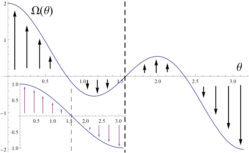
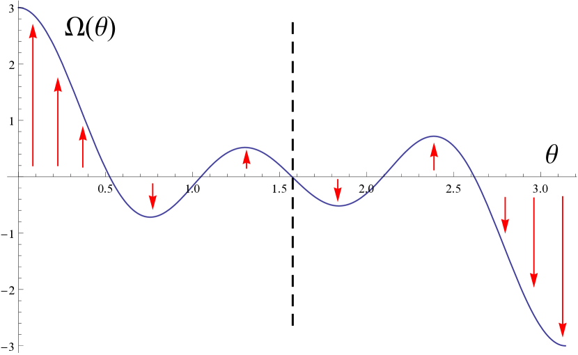
Figure 1: The differential rotation profile $\Omega$ as a function of $\theta$ with $k=4$ (left panel) and $k=6$ (right panel), respectively. In both graphs the arrow lines denote the orientation of differential rotation. The inset in the left panel shows the profile of the dipolar differential rotation.

In order to obtain the numerical solution of Einstein equation (2.2), we use the DeTurck method [19, 20, 21]. By adding a gauge fixing term to Einstein equation, we can obtain a set of elliptic equations, which are known as Einstein-DeTurk equation

$$R_{ab}+\frac{3}{L^{2}}g_{ab}-\nabla_{(a}\xi_{b)}=0,$$ (2.11)

where $\xi^{a}=g^{bc}(\Gamma^{a}_{bc}[g]-\Gamma^{a}_{bc}[\tilde{g}])$ is the Levi-Civita connection associated with a reference metric $\tilde{g}$. It is noted that reference metric $\tilde{g}$ should be choose to be as same boundary and horizon structure as $g$.

Using numerical methods for solving these equations of motion, we could obtain two classes of solutions: horizonless soliton solutions with $r_{H}=0$ and black hole solutions with $r_{H}>0$. The soliton solutions can be seen as deformations of the global Anti-de Sitter spacetime, while black hole solutions closely correspond to deformations of AdS-Schwarzschild black holes. For simplify, in our paper we only show the numerical results of the quadrupolar differential rotation $k=4$, and the cases of higher even-multipole differential rotation have similar behaviour as that of quadrupolar solution.

3 Soliton solutions

In this section, it is convenient to compactify both the radial coordinate $r$ and the polar angle coordinate $\theta$ using the change of variables $r=Ly\sqrt{2-y^{2}}/(1-y^{2})$ and $\sin\theta=1-x^{2}$, which implies that the new radial coordinate $y\in[0,1]$ and polar angle coordinate $x\in[0,1]$. Thus the inner and outer boundaries of the shell are fixed at $y=0$ and $y=1$, respectively. In order to solve the above coupled equations (2.2) numerically with a quadrupole differential rotation (2.10), we choose the ansatz of solitonic solutions as

$$\mathrm{d}s^{2}=\frac{L^{2}}{(1-y^{2})^{2}}\Bigg{\{}-U_{1}\,\mathrm{d}t^{2}+\frac{4\,U_{2}\,\mathrm{d}y^{2}}{2-y^{2}}+y^{2}(2-y^{2})\Bigg{[}\frac{4\,U_{3}}{2-x^{2}}\left(\mathrm{d}x+\frac{x}{y}\sqrt{2-x^{2}}\,\,U_{4}\,\mathrm{d}y\right)^{2}\\ +(1-x^{2})^{2}U_{5}\,\left(\mathrm{d}\phi+yx\sqrt{2-x^{2}}\left(-2+4x^{2}(2-x^{2})\right)\,U_{6}\,\mathrm{d}t\right)^{2}\Bigg{]}\Bigg{\}}\,,$$ (3.1)

where the functions $U_{i}~{}(i=1,2,3,4,5,6)$ depend on the variables $x$ and $y$. When $U_{1}=U_{2}=U_{3}=U_{5}=1$ and $U_{4}=U_{6}=0$, the metric (3.1) can reduce to Anti-de Sitter spacetime in global coordinates.

Before numerically solving the differential equations instead of seeking the analytical solutions, we should obtain the asymptotic behaviors of the six functions $U_{i}~{}(i=1,2,3,4,5,6)$, which are equivalent to know the boundary conditions we need. Because the solutions have properties of polar angle reflection symmetry $\theta\rightarrow\pi-\theta$ on the equatorial plane, it is convenient to consider the coordinate range $\theta\in[0,\pi/2]$, i.e. $x\in[0,1]$. So, we require the functions to satisfy the following Neumann boundary conditions on the equatorial plane $x=0$

$$\partial_{x}U_{i}(0,y)=0,\;\;\;i=1,2,3,4,5,6,$$ (3.2)

and set axis boundary conditions at $x=1$, where regularity must be imposed Dirichlet boundary conditions on $U_{4}$

$$U_{4}(1,y)=0,$$ (3.3)

and Neumann boundary conditions on the other functions

$$\partial_{x}U_{1}(1,y)=\partial_{x}U_{2}(1,y)=\partial_{x}U_{3}(1,y)=\partial_{x}U_{5}(1,y)=\partial_{x}U_{6}(1,y)=0.$$ (3.4)

Moreover, expanding the equations of motion near $x=1$ gives the condition $U_{3}(1,y)=U_{5}(1,y)$. In addition, the asymptotic behaviors near the conformal boundary $y=1$ are

$$U_{4}(x,1)=0,\;\;\;U_{6}(x,1)=\varepsilon,$$

$$U_{1}(x,1)=U_{2}(x,1)=U_{3}(x,1)=U_{5}(x,1)=1,$$ (3.5)

and finally, by expanding the equations of motion near $y=0$ as a power series in $y$, we have

$$\partial_{y}U_{i}(x,0)=0,\;\;\;i=1,2,3,4,5,6.$$ (3.6)

Note that in the center $y=0$ of soliton solutions, not all of the values of $U_{i}(x,0)$ are the constants independent of polar angle $x$. According to asymptotic behaviors near $y=0$, we obtain that

$$U_{1}(x,0)=c_{1},\;\;\;U_{5}(x,0)=c_{5},\;\;\;U_{6}(x,0)=c_{6},\;\;\;$$ (3.7)

$$U_{2}(x,0)=U_{2}^{(0)}(x),\;\;\;U_{3}(x,0)=U_{3}^{(0)}(x),\;\;\;U_{4}(x,0)=U_{4}^{(0)}(x),\;\;\;$$ (3.8)

where the parameters $c_{1}$, $c_{5}$ and $c_{6}$ can take arbitrary constant value, and $U^{(0)}_{2}$, $U^{(0)}_{3}$ and $U^{(0)}_{4}$ are the functions dependent of $x$.

With the above boundary conditions, the ansatz of metric has the boundary forms of Eq. (2.7) with the quadrupolar differential rotation $\Omega(\theta)=\varepsilon(\cos\theta+\cos{3\theta})$. We can choose the reference metric $\tilde{g}$ given by the line element (3.1) with $U_{4}=0,U_{6}=\varepsilon$ and $U_{1}=U_{2}=U_{3}=U_{5}=1$.

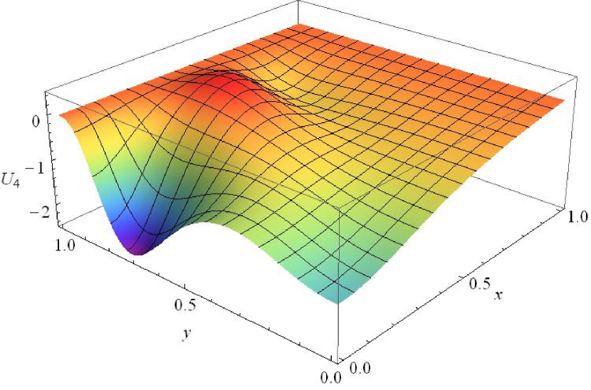
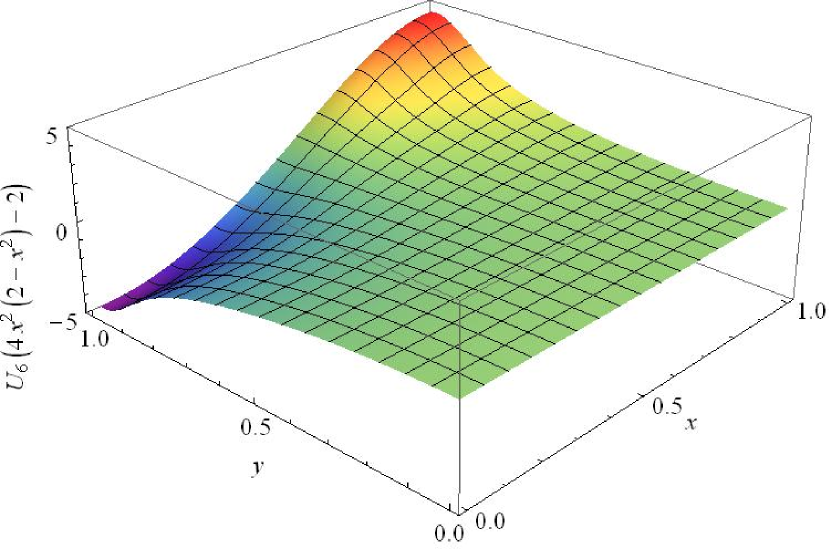
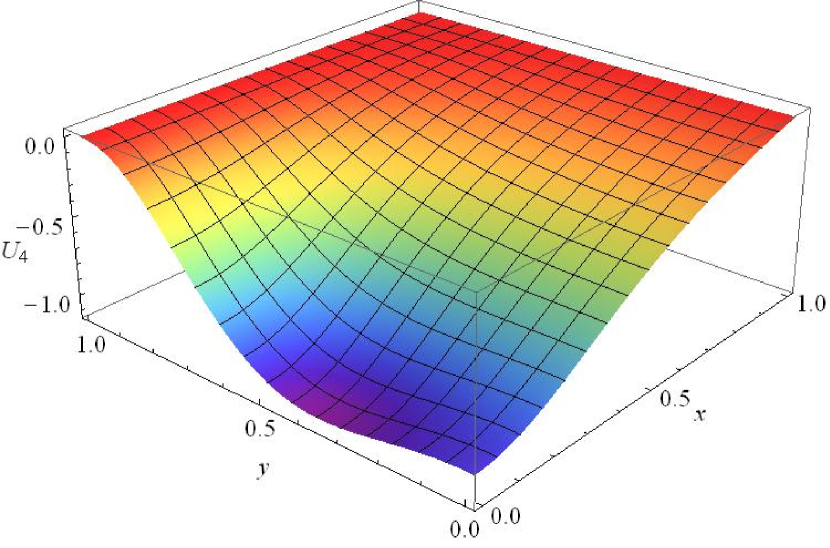
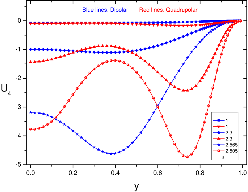
Figure 2: On the top left we show $U_{4}$ and on the top right $U_{6}(4x^{2}(2-x^{2})-2)$ of soliton solution with the quadrupolar boundary rotation, and the two figures on the top have $\varepsilon=2.3$. On the bottom left we show $U_{4}$ of soliton solution with the dipolar boundary rotation for $\varepsilon=2.3$ and on the bottom right the distribution of $U_{4}$ as a function of the $y$ coordinate in the equatorial plane at $x=0$ for various rotation parameters $\varepsilon$.

In the top of Fig. 2, we show the typical soliton result of our numerical code for $U_{4}$ in the left panel and $U_{6}(4x^{2}(2-x^{2})-2)$ in the right panel with the quadrupolar boundary rotation, and the two figures in the top have the same parameter $\varepsilon=2.3$. In order to explore the influence of the different boundary rotations on the metric, in the bottom left we show $U_{4}$ with the dipolar boundary rotation for the same paramter $\varepsilon=2.3$. Furthermore, in the bottom right the distributions of $U_{4}$ as a function of the $y$ coordinate at the equatorial plane $x=0$ for various rotation parameters $\varepsilon$ are shown, in this plot the curves $U_{4}$ with $k=2$ and $k=4$ are denoted by blue and red lines, respectively. Comparing with the results of the dipolar boundary rotation, we can see that the curve of $U_{4}$ with the quadrupolar boundary rotation have more twists and turns than that with the the dipolar boundary rotation, and the minimum value of $U_{4}$ with the quadrupolar boundary rotation is larger than that with the dipolar boundary rotation.

According to the numerical results, we find there exists stationary axisymmetric soliton solutions for $\varepsilon<\varepsilon_{c}=2.518$, where $\varepsilon_{c}$ is the maximal value and smaller than the value of dipolar boundary rotation. Moreover, the soliton solutions for each value of $\varepsilon\in(2.281,2.518)$ have two branchs.

3.1 Kretschman scalar

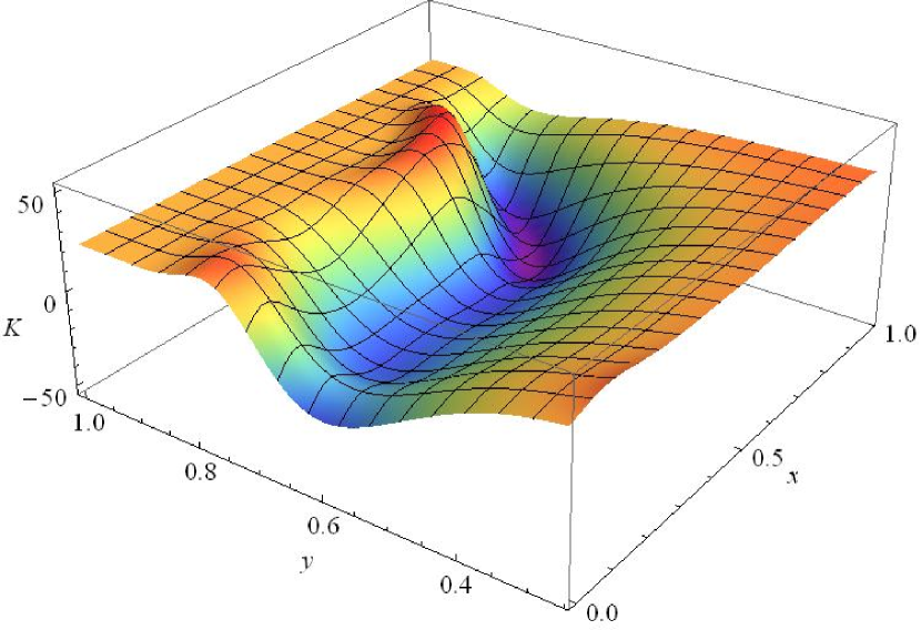
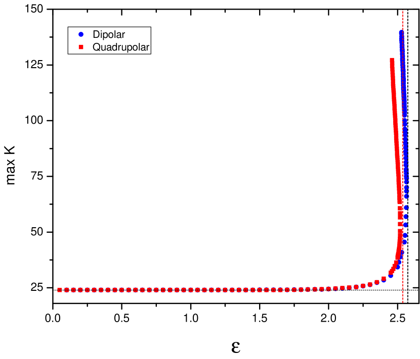
Figure 3: Right: The distribution of Kretschmann scalar as a function of $x$ and $y$ coordinate with the rotation parameter $\varepsilon=2.518$. Left: The maximum of the Kretschmann scalar as a function of the rotation parameter for the soliton solutions with $k=2,~{}4$, represented by the blue and red lines, respectively. The vertical black and red dashed gridlines indicate the $\varepsilon=2.565$ and $\varepsilon=2.518$ maximum value, respectively, and the horizon dashed black line is the value of $K=24/L^{4}$ for AdS₄ spacetime.

When one obtains a solution of Einstein equation, it is very important to know whether the spacetime of solution is regular or not. Ricci scalar is the simplest curvature invariant of a Riemannian manifold. But, considering that Ricci tensor $R$ in our model is $R=2\Lambda$, we need to choose the another invariant which can indicate the flatness of a chosen manifold. In general, one of the most useful ways is to check for the finiteness of the Kretschmann scalar, which sometimes is also called Riemann tensor squared and written as

$$K=R_{\alpha\beta\gamma\delta}R^{\alpha\beta\gamma\delta},$$ (3.9)

where $R_{\alpha\beta\gamma\delta}$ is the Riemann curvature tensor. Because it is a sum of squares of tensor components, Kretschmann scalar is a quadratic invariant.

Numerical results are presented in Fig 3. In the left panel we present the Kretschmann scalar $K$ for the quadrupolar solution with the boundary parameter $\varepsilon\simeq\varepsilon_{c}$, and it is obvious that the spacetime is not flat. In the right panel, we exhibit the maximum of the Kretschmann scalar $K$ versus the rotation parameter for the soliton solutions with $k=2,~{}4$, represented by the blue and red lines, respectively, and the critical values of the rotation parameter $k=2$ and $k=4$ are indicated by the vertical black and red dashed gridlines, respectively. From the figure, there exits the growth of Kretschmann scalar in the large branch of quadrupolar rotation solutions, which indicates the formation of a curvature singularity similar to the case of $k=2$ dipolar rotation.

3.2 Quasinormal modes

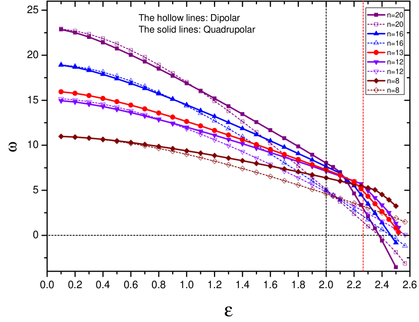
Figure 4: The normal mode frequencies $\omega$ as a function of the rotation parameter $\varepsilon$. The solid lines and dashed hollow lines stand for the quadrupolar and dipolar solutions, respectively. The vertical black and red dashed gridlines indicate the values of $\varepsilon=2$ and $\varepsilon=2.281$, respectively.

In this subsection to study the linear stability of soliton solutions with the quadrupolar rotation $k=4$, we will investigate the quasinormal modes (QNMs), which are characteristic to the background spacetimes. Following the method in papers [22, 23, 14], we consider a free, massless scalar field, obeying a massless Klein-Gordon equation

$$\nabla^{2}\chi=\frac{1}{\sqrt{-g}}\partial_{\mu}(\sqrt{-g}g^{\mu\nu}\partial_{\nu}\chi)=0,$$ (3.10)

where scalar field could be separated into the standard form

$$\chi(t,x,y,\phi)=\tilde{\chi}(x,y)e^{-i\,\omega\,t+in\phi},\,\;\;\;n=\pm 1,\pm 2,\cdots,$$ (3.11)

where the constant $\omega$ is the frequency of the complex scalar field and $n$ is the azimuthal harmonic index. With the ansatze of the soliton metric  (3.1), the scalar field could be further decomposed into

$$\tilde{\chi}(x,y)=y^{n}(1-y^{2})^{3}(1-x^{2})^{n}\psi(x,y),$$ (3.12)

where the powers of $x$ and $y$ were chosen to make function $\psi(x,y)$ to be regular at the origin. In addition, the boundary condition at $y=1$ is given by

$$\partial_{y}\psi(x,y)=-|n|\,\psi(x,y).$$ (3.13)

At $y=0$ and $x=\pm 1$, we require that the function $\psi(x,y)$ approaches the homogeneous solution with Neumann boundary conditions.

In the Fig 4, we plot the normal mode frequencies $\omega$ as a function of the rotation parameter $\varepsilon$ for the corresponding values of $n$, represented by solid lines. Meanwhile, we also show the numerical results of QNMs studied in [14], represented by dashed lines. We can see that normal mode frequencies $\omega$ with $n\leq 13$ are always positive modes in the spectrum of perturbations, while, the frequency becomes negative at a specific value of $\varepsilon$ when $n\geq n_{c}=14$. One can expect some branches of soliton solution with scalar hair $\chi$ condensation can be found. Comparing with the results of the dipolar differential rotation $k=2$, we see that the azimuthal harmonic index $n_{c}=14$ of the quadrupolar differential rotation is larger than the index $n_{c}=13$ of the dipolar differential rotation.

4 Black hole solutions

Figure 5: Top left: The distributions of $U_{4}$ as a function of $x$ and $y$ for large black hole with quadrupolar rotation parameter $\varepsilon=2.215$. Top right: For large black hole, the distributions of $U_{4}$ as a function of $y$ at the equatorial plane for various values of $\varepsilon$. Bottom left: The distributions of $U_{4}$ for small black hole with quadrupolar rotation parameter $\varepsilon=2.5$. Bottom right: For small black hole, the distributions of $U_{4}$ as a function of $y$ at the equatorial plane for various values of $\varepsilon$. In both right panels, the red and blue lines correspond to quadrupolar and dipolar rotation, respectively.

In this section, it is convenient to compactify the radial coordinate $r$ and polar angle coordinate $\theta$ with the change of variables $r=Ly_{p}/(1-y^{2})$ and $\sin\theta=1-x^{2}$, respectively. In order to obtain the black hole solutions with quadrupolar differential rotation, we consider the ansatz of metric

$$\mathrm{d}s^{2}=\frac{L^{2}}{(1-y^{2})^{2}}\Bigg{\{}-y^{2}\Gamma^{+}(y)U_{1}\mathrm{d}t^{2}+\frac{4\,y_{p}^{2}U_{2}\,\mathrm{d}y^{2}}{\Gamma^{+}(y)}\\ +y_{p}^{2}\Bigg{[}\frac{4\,U_{3}}{2-x^{2}}\left(\mathrm{d}x+yx\sqrt{2-x^{2}}\left(-2+4x^{2}(2-x^{2})\right)\,U_{4}\,\mathrm{d}y\right)^{2}\\ +(1-x^{2})^{2}U_{5}\,\left(\mathrm{d}\phi+y^{2}x\sqrt{2-x^{2}}\left(-2+4x^{2}(2-x^{2})\right)U_{6}\,\mathrm{d}t\right)^{2}\Bigg{]}\Bigg{\}},$$ (4.1a)

with

$$\Gamma(y)=(1-y^{2})^{2}+y_{p}^{2}(3-3y^{2}+y^{4})\,,\quad\text{and}\quad\Gamma^{+}(y)=\Gamma(y)\delta+y_{p}^{2}(1-\delta)\,,$$ (4.1b)

where the functions $U_{i}(x,y)~{}(i=1,2,3,4,5,6)$ depend on the variables $x$ and $y$. Providing that $U_{4}=U_{6}=0$ and $U_{1}=U_{2}=U_{3}=U_{5}=\delta=1$, the metric (4.1a) reduces to the Schwarzschild-AdS black hole.

In the ansatz (4.1a), we have three parameters: $\varepsilon$, which sets the amplitude of the boundary rotation, and $(y_{p},\delta)$, which determine the black hole temperature. The Hawking temperature of the black hole with quadrupolar differential rotation is given by

$$T=\frac{1}{4\pi}\sqrt{-g^{tt}g^{\alpha\beta}\partial_{\alpha}g_{tt}\partial_{\beta}g_{tt}}\mid_{y=0}=\frac{(\delta+2{\delta}y_{p}^{2}+y_{p}^{2})}{4{\pi}y_{p}},$$ (4.2)

where the parameter $\delta$ is introduced to control the temperature to any values. If $\delta=1$, the temperature has a minimum at $y_{p}=1/\sqrt{3}$, coinciding with the minimal temperature of a Schwarzschild-AdS₄, occurring at $T_{c}\equiv\sqrt{3}/(2\pi)\approx 0.2757$. It is obvious that the black hole temperature with quadrupolar differential rotation in (4.2) is same as that with dipolar differential rotation. When $\delta$ have a fixed value, one can obtain two solutions with the same temperature, which we call as large black holes with larger $y_{p}$, and small black holes with smaller $y_{p}$.

The boundary condition is similar to the soliton case. At $x=0$ and $y=0$, the functions $U_{i}$ satisfy the following Neumann boundary conditions

$$\partial_{x}U_{i}(0,y)=\partial_{y}U_{i}(x,0)=0,\;\;\;i=1,2,3,4,5,6,$$ (4.3)

and at axis boundary $x=1$ , we require that regularity must be imposed with $U_{4}=0,U_{3}=U_{5}$, and $\partial_{x}U_{1}=\partial_{x}U_{2}=\partial_{x}U_{3}=\partial_{x}U_{5}=\partial_{x}U_{6}=0$. At the conformal boundary $y=1$, we set $U_{4}=0,U_{6}=\varepsilon\,\,,\text{and}\,U_{2}=U_{3}=U_{5}=1$. Moreover, expanding the equations of motion near $y=0$ gives $U_{1}(x,0)=U_{2}(x,0)$. The reference metric $\tilde{g}$ to be given by the line element (4.1a) with $U_{4}=0,U_{6}=\varepsilon$ and $U_{1}=U_{2}=U_{3}=U_{5}=1$.

In the left panels of Fig. 5, we show the typical quadrupolar rotation results of $U_{4}$ for large black hole in the right top panel and for small black hole in the right bettom panel, which correspond to $\varepsilon=2.215$ and $\varepsilon=2.5$, respectively. In order to compare with the results of the dipolar different boundary rotations for the large black hole, in the top right we show the distributions of $U_{4}$ as a function of the $y$ coordinate at the equatorial plane $x=0$ for various values of $\varepsilon$ with quadrupolar (red lines) and dipolar ( blue lines) rotation, respectively. Meanwhile, in the bottom right the distributions of $U_{4}$ for small black hole are shown. From two plots in the left panels, we can see that the deformation of the curve of $U_{4}$ arose with the increasing $\varepsilon$, and the curves of the quadrupolar rotation have also more twists and turns than that with the dipolar rotation, which is similar to the soliton case.

4.1 Entropy

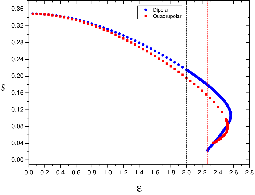
Figure 6: Entropy versus the parameter $\varepsilon$ for the small and large branches of black hole solutions with a temperature $T=1/\pi$. Left: The large black hole of dipolar (blue line) and quadrupolar (red line) differential rotation with $y_{p}=1$ are shown. Right: The small black hole of dipolar and quadrupolar differential rotation with $y_{p}=1/3$ is shown with blue and red lines, respectively. The horizonal black dashed gridlines marks the entropy $S=0$. In both panels the vertical black and red dashed gridlines indicate the $\varepsilon=2$ and $\varepsilon=2.281$ maximum value, respectively.

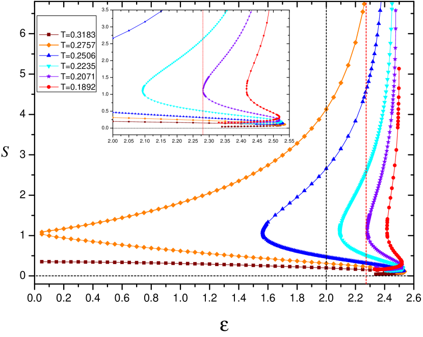
Figure 7: Entropy versus the parameter $\varepsilon$ for low temperature black holes with $T<T_{c}\simeq 0.2757$. The brown squares show the small black holes with $T=1/\pi$, the vertical black and red dashed gridlines indicate the $\varepsilon=2$ and $\varepsilon=2.281$ maximum value, respectively.

In this section we discuss the entropy of deforming black holes with quadrupolar differential rotation, which is proportional to the area of event horizon and given by

$$S=\frac{A}{4G_{N}}=\frac{2\pi\,y_{p}^{2}\,L^{2}}{G_{N}}\int_{0}^{1}\mathrm{d}x\frac{1-x^{2}}{\sqrt{2-x^{2}}}\sqrt{U_{3}(x,0)U_{5}(x,0)}\,.$$ (4.4)

In Fig. 6, we show entropy versus the parameter $\varepsilon$ for the small and large branches of black hole solutions with the temperature $T=1/\pi$. The large black hole with $y_{p}=1$ is shown in the left panel, where the red and blue lines correspond to black holes with quadrupolar and dipolar differential rotation, respectively. The vertical red dashed gridlines indicate the $\varepsilon=2.281$ maximum value beyond which one cannot find axially symmetric black hole solutions with quadrupolar differential rotation. Meanwhile, the vertical black dashed gridlines indicates the $\varepsilon=2$ maximum value of solutions with dipolar differential rotation. For the large black holes with quadrupolar differential rotation, the entropy always increases with the increasing of $\varepsilon$, which is similar as the case of dipolar differential rotation. For the small black hole with $y_{p}=1/3$ in the right panel, the red and blue lines correspond to solutions with quadrupolar and dipolar differential rotation, respectively. With the increasing of $\varepsilon$, the entropy of black hole with quadrupolar differential rotation decreases firstly and then reaches a maximum point of of $\varepsilon$. Further decreasing $\varepsilon$, one can find another branch of small black holes in which the entropy continues to decrease.

Comparing with the results of dipolar differential rotation, we find that the norm of Killing vector $\partial_{t}$ in Eq. (2.9) becomes spacelike for certain regions of $\theta$ when $\varepsilon\in(2,2.281)$, however, black holes with quadrupolar differential rotation do not develop hair due to superradiance, which was different from the case of dipolar rotation. At the fixed temperature $T>T_{c}\equiv\sqrt{3}/(2\pi)\approx 0.2757$, the entropies of the large and small black hole have the similar behaviors as those in Fig. 6. In order to study the solutions at $T<T_{c}\equiv\sqrt{3}/(2\pi)$, we fix the value of the temperature with $\delta<1$. When $\delta\rightarrow 0$, the deformed black holes can have a minimum temperature arbitrarily close to zero temperature.

In Fig. 7, the entropy against the deforming parameter for low temperature black holes with $T<T_{c}\equiv\sqrt{3}/(2\pi)$ is shown. The vertical black and red dashed gridlines indicate the $\varepsilon=2$ and $\varepsilon=2.281$, respectively. and the brown squares represent the small black holes with $T=1/\pi$, which has been discussed in Fig. 6. The orange disks show black holes with the critical temerature $T_{c}\simeq 0.2757$, and two branches of black holes at critical temperature begin to connect and form a curve. As the temperature continue to decrease, the turning point corresponds to higher values of $\varepsilon$.

4.2 Horizon geometry

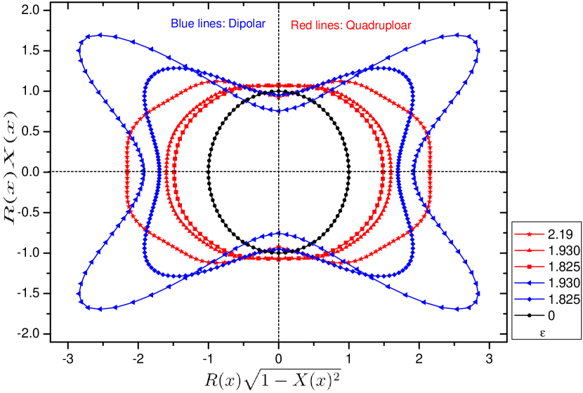
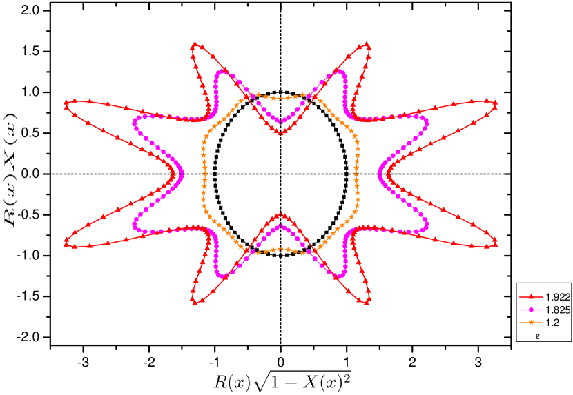
Figure 8: Left: Hyperbolic embedding of the cross section of the black hole horizons at the temperature $T=1/\pi$. The blue and red lines correspond to dipolar and quadrupolar rotation, respectively. Right: Hyperbolic embedding of the cross section of the black hole horizons at the temperature $T=2/\pi$. In both panels the black dashed lines represent the Schwarzschild-AdS black hole at the temperature $T=1/\pi$.

Though the numerical results of the metric (4.1a) are obtained in last section, one typically has little information about the real geometry features of even horizons of deforming black hole in coordinate space. In order to see how the deforming boundary affects the geometric features of the event horizon, we can investigate the geometry of a two-dimensional surface in a curved space by using an isometric embedding in the three-dimensional space [24, 25, 26, 27, 28], which has been introduced to study the horizon with dipolar rotation embedding in hyperbolic space[29, 14]. In the polar coordinates, the metric of hyperbolic three-dimensional space $\mathbb{H}^{3}$ is given by

$$\mathrm{d}s^{2}_{\mathbb{H}^{3}}=\frac{\mathrm{d}R^{2}}{1+R^{2}/\tilde{\ell}^{2}}+R^{2}\left[\frac{\mathrm{d}X^{2}}{1-X^{2}}+(1-X^{2})\,\mathrm{d}\phi^{2}\right],$$ (4.5)

where $\tilde{\ell}$ is the radius of the hyperbolic space, and the induced metric on the horizon of the black hole with the metric (4.1a) is given by

$$\mathrm{d}s^{2}_{H}=L^{2}\left[\frac{4y_{p}^{2}U_{3}(x,0)}{2-x^{2}}\,\mathrm{d}x^{2}+y_{p}^{2}(1-x^{2})^{2}U_{5}(x,0)\,\mathrm{d}\phi^{2}\right],$$ (4.6)

and with the pull back of line element (4.5) on the induced metric (4.6), one can obtain a embedding of two-dimensional line element, which is given by a parametric curve $\{R(x),X(x)\}$.

The numerical results of hyperbolic embedding of the cross section of the event horizons for several values of $\varepsilon$ are presented in Fig. 8. In order to compare with the results of dipolar rotation in [14], we also adopt the same parameter $\tilde{\ell}=0.73$. In the left panel, we fix the black hole temperature to be $T=1/\pi$, the black line represents the curve of Schwarzschild-AdS black hole with $\varepsilon=0$. The blue and red lines correspond to dipolar and quadrupolar rotation, respectively. As one increases $\varepsilon$, the horizon cross section begin to deform and has the four arms of the horizon cross section, which are taken further apart and form the quadrupolar structure. Comparing with the dipolar rotation, the deformation of quadrupolar rotation is small. In the right panel, at the temperature $T=2/\pi$, we recalculate the embedding of the cross section and obtain the larger deformation of quadrupolar rotation.

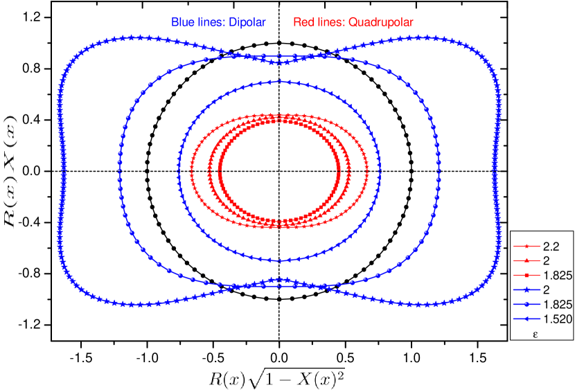
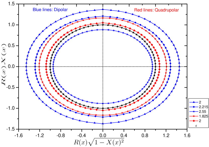
Figure 9: Hyperbolic embedding of the cross section of the black hole solution horizons with low temperature $T=0.2506<T_{c}$. The black circle represents the black hole with $\varepsilon=0$ at the temperature $T=1/\pi$. Left: Embeddings for the large black hole solutions. Right: Embeddings for the small black hole branches. In both panels the blue lines represent dipolar rotation as well as the red lines represent quadrupolar rotation.

In  Fig. 9, we set a low temperature $T=0.2506$, and find that the deformation of quadrupolar rotation is smaller with the decrease of temperature. Moreover, the geometry of the horizon cross section shrink to the interior. Comparing with the curve of the large black hole in the left panel, the small black hole have nearly circular curve. At the same temperature, the curve of quadrupolar rotation is closer to the interior than that of dipolar rotation.

4.3 Quasinormal modes

In this subsection we will discuss the linear stability of deforming black hole with quadrupolar rotation by studying the quasinormal modes.

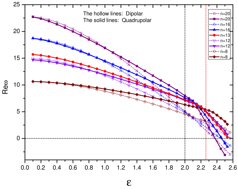
Figure 10: The real part of frequencies $\omega$ as a function of the deforming parameter $\varepsilon$. The solid lines and dashed hollow lines stand for the quadrupolar and dipolar solutions, respectively. The vertical black and red dashed gridlines indicate the $\varepsilon=2$ and $\varepsilon=2.281$, respectively.

With the ansatze of the black hole metric  (4.1a), the scalar field imposed regularity in ingoing Eddington-Finkelstein coordinates [30, 31] could be decomposed into

$$\chi(t,x,y,\chi)=e^{i(-\omega t+n\chi)}y^{-i\frac{2\omega y_{p}}{1+3y_{p}^{2}}}(1-y^{2})^{3}(1-x^{2})^{|n|}\psi(x,y)\,,$$ (4.7)

where the powers of $x$ and $y$ were chosen to make function $\psi(x,y)$ to be regular at the origin. At $y=0$ and $x=\pm 1$, we require that the function $\psi(x,y)$ approach the homogeneous solution with Neumann boundary conditions. In addition, the boundary conditions at $y=1$ are given by

$$\partial_{y}\psi(x,1)=\frac{2i\,y_{p}\omega}{(1+3y_{p}^{2})}\psi(x,1).$$ (4.8)

In the Fig 10, for a small black black hole at $T=1/\pi$, we plot the real part of frequencies $\omega$ as a function of the deforming parameter $\varepsilon$ for the corresponding values of $n$, represented by solid lines. In addition, we also plot the curve of QNMs with dipolar rotation studied in [14], represented by dashed hollow lines. The vertical black and red dashed gridlines indicate the $\varepsilon=2$ and $\varepsilon=2.281$, respectively, and the horizonal black dashed gridlines shows where Re $\omega$ = 0. From the figure, we can see that frequencies Re $\omega$ with $n\leq 13$ are always positive values in the spectrum of perturbations, while the frequency begin to be negative at a specific value of $\varepsilon$ when $n\geq n_{c}=14$. The characteristic of Re $\omega$ against the boundary rotation parameter $\varepsilon$ is similar to that of soliton solutions. For the first unstable mode at $m=14$, one can expect some branches of black hole with scalar hair $\Phi$ condensation can be found.

5 Conclusions

In this paper, we analyzed the conformal boundary of four dimensional static asymptotically AdS solutions in Einstein gravity and numerically constructed the solutions of compact objects with even multipolar differential rotation boundary, including solitons and black holes. Comparing with the dipolar differential rotation solutions in [14], we found that for high temperature black holes with $T>T_{c}\simeq 0.2757$, the norm of Killing vector $\partial_{t}$ becomes spacelike for certain regions of $\theta$ when $\varepsilon\in(2,2.281)$, however, solitons and black holes with quadrupolar differential rotation do not develop hair due to superradiance, which was different from the case of dipolar rotation. For the large black holes of the high temperature, we did not find any solutions which could cross $\varepsilon\in 2.281$. Furthermore, with the isometric embedding of horizon, it is clearly seen that black hole horizon is deformed into four hourglass shapes. In addition, we also study the numerical solutions of the entropies of the large and small black hole, which have the similar behaviors as that of dipolar differential rotation. By studying the quasinormal modes, we discussed the linear stability of deforming solitons and black holes with quadrupolar rotation, respectively, and found that for some branches of solution with scalar hair $\Phi$ condensation, the minimal azimuthal harmonic index $n_{c}=14$ of the quadrupolar differential rotation is larger than $n_{c}=13$ of the dipolar differential rotation.

It is interesting to find that even though the norm of Killing vector $\partial_{t}$ becomes spacelike for certain regions of $\theta$ when $\varepsilon>2$, solitons and black holes with quadrupolar differential rotation still exist and do not develop hair due to superradiance. We also check the numerical solutions with hexapolar differential rotation, which show very similar results to quadrupolar differential rotation. There exists the solution of hexapolar differential rotation when $\varepsilon>2$.

There are several interesting extensions of our work. First, we have studied the deforming black holes with even multipolar differential rotation boundary, next, we will investigate black holes with odd multipolar differential rotation boundary, which has the symmetric rotation profile with respect to reflections on the equatorial plane. There exists a question whether total angular momentum of black hole is non-zero. The second extension of our study is to consider the action of Einstein-Maxwell gravity in AdS spacetime and construct the deforming charged black holes. Due to the existence of charges, at the same temperature, one finds that there are three branches of solutions and the phase diagram of solutions is more intricate than that without charges. Finally, we are planning to extend the study of the deforming black holes to the five-dimensional solutions in future work.

References

- [1] W. Israel, “Event Horizons in Static Vacuum Space-Times,” Phys. Rev. 164, 1776 (1967).
- [2] R. Ruffini and J. A.Wheeler, “Introducing the black hole,” Phys. Today 24, 30 (1971).
- [3] B. Carter, C. De Witt, and B. S. De Witt, in Proceedings of 1972 Session of Ecole d Ete De Physique Theorique, (Gordon and Breach, New York, 1973).
- [4] P. T. Chrusciel, J. Lopes Costa and M. Heusler, “Stationary Black Holes: Uniqueness and Beyond,” Living Rev. Rel. 15, 7 (2012) [arXiv:1205.6112 [gr-qc]].
- [5] J. M. Maldacena, “ The large limit of superconformal field theories and supergravity,” Int. J. Theor. Phys. 38, 1113 (1999).
- [6] J. M. Maldacena, “The Large N limit of superconformal field theories and supergravity,” Int. J. Theor. Phys. 38, 1113 (1999) [Adv. Theor. Math. Phys. 2, 231 (1998)] doi:10.1023/A:1026654312961, 10.4310/ATMP.1998.v2.n2.a1 [hep-th/9711200].
- [7] E. Witten, “Anti-de Sitter space and holography,” Adv. Theor. Math. Phys. 2, 253 (1998) doi:10.4310/ATMP.1998.v2.n2.a2 [hep-th/9802150].
- [8] O. Aharony, S. S. Gubser, J. M. Maldacena, H. Ooguri and Y. Oz, “Large N field theories, string theory and gravity,” Phys. Rept. 323, 183 (2000) doi:10.1016/S0370-1573(99)00083-6 [hep-th/9905111].
- [9] Y. Chen, Y. K. Lim and E. Teo, “Deformed hyperbolic black holes,” Phys. Rev. D 92, no. 4, 044058 (2015) doi:10.1103/PhysRevD.92.044058 [arXiv:1507.02416 [gr-qc]].
- [10] T. Levi-Civita, “Nontrivial, static, geodesically complete, vacuum space-times with a negative cosmological constant,” Rend. Acc. Lincei, 26, 307 (1917), 27, 3, 183, 220, 240, 283, 343 (1918), 28, 3, 101 (1919).
- [11] H. Weyl, “Nontrivial, static, geodesically complete, vacuum space-times with a negative cosmological constant,” Ann. Phys. 54, 117 (1917).
- [12] J. F. Plebanski and M. Demianski, “Rotating, charged, and uniformly accelerating mass in general relativity,” Annals Phys. 98, 98 (1976). doi:10.1016/0003-4916(76)90240-2
- [13] Y. Chen and E. Teo, “Black holes with bottle-shaped horizons,” Phys. Rev. D 93, no. 12, 124028 (2016) doi:10.1103/PhysRevD.93.124028 [arXiv:1604.07527 [gr-qc]].
- [14] J. Markeviit and J. E. Santos, “Stirring a black hole,” JHEP 1802, 060 (2018) doi:10.1007/JHEP02(2018)060 [arXiv:1712.07648 [hep-th]].
- [15] S. R. Green, S. Hollands, A. Ishibashi and R. M. Wald, “Superradiant instabilities of asymptotically anti-de Sitter black holes,” Class. Quant. Grav. 33, no. 12, 125022 (2016) doi:10.1088/0264-9381/33/12/125022 [arXiv:1512.02644 [gr-qc]].
- [16] T. Crisford, G. T. Horowitz and J. E. Santos, “Attempts at vacuum counterexamples to cosmic censorship in AdS,” JHEP 1902, 092 (2019) doi:10.1007/JHEP02(2019)092 [arXiv:1805.06469 [hep-th]].
- [17] G. T. Horowitz, J. E. Santos and C. Toldo, “Deforming black holes in AdS,” JHEP 1811, 146 (2018) doi:10.1007/JHEP11(2018)146 [arXiv:1809.04081 [hep-th]].
- [18] J. L. Bl zquez-Salcedo, J. Kunz, F. Navarro-L rida and E. Radu, “New black holes in minimal gauged supergravity: Deformed boundaries and frozen horizons,” Phys. Rev. D 97, no. 8, 081502 (2018) doi:10.1103/PhysRevD.97.081502 [arXiv:1711.08292 [gr-qc]].
- [19] M. Headrick, S. Kitchen and T. Wiseman, “A New approach to static numerical relativity, and its application to Kaluza-Klein black holes,” Class. Quant. Grav. 27, 035002 (2010) doi:10.1088/0264-9381/27/3/035002 [arXiv:0905.1822 [gr-qc]].
- [20] T. Wiseman, Numerical construction of static and stationary black holes, in Black holes in higher dimensions, G. Horowitz ed., Cambridge University Press, Cambridge U.K. (2012).
- [21] O. J. C. Dias, J. E. Santos and B. Way, “Numerical Methods for Finding Stationary Gravitational Solutions,” Class. Quant. Grav. 33, no. 13, 133001 (2016) doi:10.1088/0264-9381/33/13/133001 [arXiv:1510.02804 [hep-th]].
- [22] O. J. C. Dias and J. E. Santos, “Boundary Conditions for Kerr-AdS Perturbations,” JHEP 1310, 156 (2013) doi:10.1007/JHEP10(2013)156 [arXiv:1302.1580 [hep-th]].
- [23] V. Cardoso, O. J. C. Dias, G. S. Hartnett, L. Lehner and J. E. Santos, “Holographic thermalization, quasinormal modes and superradiance in Kerr-AdS,” JHEP 1404, 183 (2014) doi:10.1007/JHEP04(2014)183 [arXiv:1312.5323 [hep-th]].
- [24] L. Flamm, “Beiträge zur Einsteinischen Gravitationtheorie,” Physikalische. Zeitschrift 17 (1916) 448-454 (in particular p. 450).
- [25] L. Smarr, “Surface Geometry of Charged Rotating Black Holes,” Phys. Rev. D 7 (1973) 289.
- [26] A. Friedman, “Isometric Embeddings of Riemannian manifolds into Euclidean spaces,” Rev. Mod. Phys. 37 (1965) 201.
- [27] J. Rosen, “Embedding various relativistic Riemannian spaces in Pseudo-Euclidean spaces,” Rev. Mod. Phys. 37 (1965) 204.
- [28] H. Goenner, “Local isometric embedding of Riemannian manifolds and Einstein’s theory of gravitation”, in General Relativity and Gravitation: One hundred years after the birth of Einstein, Edited by A.Held, Vol.1, Plenum Press, 1980.
- [29] G. W. Gibbons, C. A. R. Herdeiro and C. Rebelo, “Global embedding of the Kerr black hole event horizon into hyperbolic 3-space,” Phys. Rev. D 80, 044014 (2009) doi:10.1103/PhysRevD.80.044014 [arXiv:0906.2768 [gr-qc]].
- [30] G. T. Horowitz and V. E. Hubeny, “Quasinormal modes of AdS black holes and the approach to thermal equilibrium,” Phys. Rev. D 62, 024027 (2000) doi:10.1103/PhysRevD.62.024027 [hep-th/9909056].
- [31] E. Berti, V. Cardoso and A. O. Starinets, “Quasinormal modes of black holes and black branes,” Class. Quant. Grav. 26, 163001 (2009) doi:10.1088/0264-9381/26/16/163001 [arXiv:0905.2975 [gr-qc]].