A Novel Statistical Method for Measuring the Temperature-Density Relation in the IGM
Using the $b$-$N_{\text{HI}}$ Distribution of absorbers in the Lyα Forest

Abstract

We present a new method for determining the thermal state of the intergalactic medium based on Voigt profile decomposition of the Ly$\alpha$ forest. The distribution of Doppler parameter and column density ($b$-$N_{\text{HI}}$ distribution) is sensitive to the temperature density relation $T=T_{0}(\rho/{\rho_{0}})^{\gamma-1}$, and previous work has inferred $T_{0}$ and $\gamma$ by fitting its low-$b$ cutoff. This approach discards the majority of available data, and is susceptible to systematics related to cutoff determination. We present a method that exploits all information encoded in the $b$-$N_{\text{HI}}$ distribution by modeling its entire shape. We apply kernel density estimation to discrete absorption lines to generate model probability density functions, then use principal component decomposition to create an emulator which can be evaluated anywhere in thermal parameter space. We introduce a Bayesian likelihood based on these models enabling parameter inference via Markov chain Monte Carlo. The method’s robustness is tested by applying it to a large grid of thermal history simulations. By conducting 160 mock measurements we establish that our approach delivers unbiased estimates and valid uncertainties for a 2D $(T_{0},\gamma)$ measurement. Furthermore, we conduct a pilot study applying this methodology to real observational data at $z=2$. Using 200 absorbers, equivalent in pathlength to a single Ly$\alpha$ forest spectrum, we measure $\log T_{0}=4.092^{+0.050}_{-0.055}$ and $\gamma=1.49^{+0.073}_{-0.074}$ in excellent agreement with cutoff fitting determinations using the same data. Our method is far more sensitive than cutoff fitting, enabling measurements of $\log T_{0}$ and $\gamma$ with precision on $\log T_{0}$ ($\gamma$) nearly two (three) times higher for current dataset sizes.

tablenum SIXtablenum

1 Introduction

The low density intergalactic medium (IGM) is the major reservoir of baryonic matter in the Universe. As the universe undergoes phase transitions, such as a global reionization process, the thermal state of the IGM is changed. Thus precise measurements of the thermal history of the IGM are key for our understanding of the details of reionization processes in the universe.

The established picture concerning reionization is that the universe undergoes two major phase transitions that change the thermal state of the baryons. Firstly the reionization of hydrogen (H I$\rightarrow$H II) which is believed to be completed by redshift $z\sim 6$ (McGreer et al. 2015). This reionization process is believed to be driven by the first galaxies (Faucher-Giguère et al. 2008a; Robertson et al. 2015), but it has recently been debated whether early QSOs (quasi stellar objects, or quasars) could have contributed substantially (Madau & Haardt 2015; Khaire et al. 2016; Kulkarni et al. 2018).

Once the population of luminous QSOs becomes abundant, there are enough high energy photons available to power a second phase transition, namely the second reionization of Helium (He II$\rightarrow$He III) (see e.g. Madau & Meiksin 1994; Miralda-Escudé et al. 2000; McQuinn et al. 2009; Dixon & Furlanetto 2009; Compostella et al. 2013, 2014; Syphers & Shull 2014; Dixon et al. 2014). Due to the requirement of a large QSO population, this process becomes only possible at much later times and is expected to be completed by $z\simeq 2.7$ (see e.g. Worseck et al. 2011, 2018). Understanding the thermal imprint of these processes is key for understanding the details of reionization processes, i.e. their evolution and the sources powering them.

The main driving forces governing the thermal state of the IGM (at $z\lesssim 5$) are heating caused by photoionization by the ultraviolet background (UVB) and adiabatic cooling due to the expansion of the universe. It can be shown that long after the impulsive heating by reionization events (McQuinn et al. 2009; Compostella et al. 2013; McQuinn & Upton Sanderbeck 2016), the majority of the gas is naturally driven to a tight temperature-density relation (TDR) with the form $T=T_{0}(\rho/\rho_{0})^{\gamma-1}$ (Hui & Gnedin 1997), where $T_{0}$ is the temperature at mean density $\rho_{0}$, and the power law index $\gamma$ quantifies the temperature contrast between underdensities and overdensities.

Since intergalactic gas is so diffuse, it is extremely challenging to study its properties in emission. Therefore, most of the knowledge we have about the IGM comes from observing it in absorption. The primary observable at $z\lesssim 6$ that contains information about the thermal state of the IGM is the Lyman-$\alpha$ (Ly$\alpha$) forest (Gunn & Peterson 1965; Lynds 1971). This fluctuating absorption, consisting of a series of redshifted Ly$\alpha$ absorption features in the lines of sight toward luminous objects (QSOs), arises from the fact that residual neutral hydrogen is present in the diffuse IGM. The Ly$\alpha$ forest can be used in different ways as a probe of the thermal state of the intergalactic gas. This includes various statistical measures such as of the power spectrum of the transmitted flux (e.g. Zaldarriaga et al. 2001; McDonald et al. 2006; Walther et al. 2018a; Khaire et al. 2018; Walther et al. 2018b; Boera et al. 2018), the curvature statistic (Becker et al. 2011; Boera et al. 2014), the flux probability distribution function (e.g. Bolton et al. 2008; Viel et al. 2009; Lee et al. 2015), as well as wavelet decompositions of the forest (e.g. Theuns et al. 2002; Lidz et al. 2010; Garzilli et al. 2012).

In this study we use a method that treats the Ly$\alpha$ forest as a superposition of multiple discrete absorption profiles (Schaye et al. 1999; Ricotti et al. 2000; McDonald et al. 2001), whereby each absorption profile is described by its position in redshift space, a Doppler parameter $b$ describing the absorption line width, and a column density $N_{\text{HI}}$ that characterizes the density along the line of sight causing the absorption. The thermal state is encoded in the absorption profiles, as thermal random motions in the absorbing gas contribute to the Doppler parameter. This is simply a result of blue and redshifting of the absorption wavelength due to Maxwell-Boltzmann velocity distributions in the gas. Additionally, the broadening of absorption profiles is increased by the by differential Hubble flow across the spatial extent of the absorber, set by the pressure smoothing scale $\lambda_{P}$ (Gnedin & Hui 1998a; Schaye 2001; Peeples et al. 2010; Rorai et al. 2013a; Kulkarni et al. 2015; Rorai et al. 2017). Peculiar velocity structure along the line of sight also contributes to the width of absorbers.

The conventional method for measuring thermal parameters using the joint distribution of column densities and Doppler parameters ($b$-$N_{\text{HI}}$ distribution) of absorbers in the Ly$\alpha$ forest in a particular redshift interval relies on the measurement of the thermal state dependent lower cutoff in this distribution (see Schaye et al. 1999; Ricotti et al. 2000; McDonald et al. 2001; Schaye et al. 2000; Rudie et al. 2012; Bolton et al. 2014; Garzilli et al. 2015; Rorai et al. 2018; Hiss et al. 2018; Telikova et al. 2018; Garzilli et al. 2018), set primarily by the minimal broadening associated with the temperature of the absorbers.

Although it constitutes a powerful tool for measuring the thermal state of the gas, the cutoff fitting technique has a series of inherent disadvantages. The main one being that the position of the cutoff is fitted using an iterative technique which excludes absorbers from the distribution. This means that a small number of absorbers is effectively used for measuring the position of the cutoff, resulting in diminished sensitivity of the method on the total number of absorbers in the dataset once the distribution is well populated (Schaye et al. 1999). In addition, narrow metal line absorbers, which are difficult to completely identify and mask, can result in significant contamination around the cutoff, compromising the precision with which the cutoff can be determined, and adding systematics which are difficult to control. Another complication of this method, as shown in Hiss et al. (2018) in the context of the comparison with the results by Rorai et al. (2018), is that choice of cutoff fitting method (i.e. least-squares or mean-deviation minimization) can lead to significantly different $T_{0}$ and $\gamma$ measurements. All of these problems call for a new method for interpreting the information about the thermal state of the IGM encoded in the $b$-$N_{\text{HI}}$ distribution.

In this work we introduce, test, and apply a new method for constraining $T_{0}$ and $\gamma$ using the $b$-$N_{\text{HI}}$ distribution. The main difference with the traditional cutoff fitting approach is that we model the entire distribution, and thus bypass the complications associated with quantifying the position of a lower cutoff. While other studies employed a parametric description of the full $b$-$N_{\text{HI}}$ distribution in order to carry out measurements of the parameters of the TDR (see e.g. Ricotti et al. 2000; Telikova et al. 2018), we instead construct smooth probability density functions (PDF) of simulated $b$-$N_{\text{HI}}$ distributions using a non-parametric approach. These PDFs can then be used as models for conducting inference. The reader should keep in mind that all results presented in our proof of concept concern $T_{0}$ and $\gamma$ alone and do not marginalize over other parameters. All results presented should be interpreted as a demonstration of the capabilities of this new approach rather than a perfect measurement.

This paper is structured as follows. We introduce our simulations and mock data generation in § 2. Our new method for constructing a model of the $b$-$N_{\text{HI}}$ distribution and inferring thermal parameters is described in § 3. In § 4, we carry out measurements using different mock data realizations at $z=2$ to explore the robustness of this technique. We carry out a pilot study of this new method in § 5, where real observational data at $z=2$ is compared to a grid of hydrodynamical simulations. We discuss and summarize our results in § 6.

2 Simulations

In this section we describe how we generate simulated Ly$\alpha$ forest spectra with different combinations of the underlying thermal parameters that govern the IGM. Specifically, we wish to generate a grid of $T_{0},\gamma$ at a fixed $\lambda_{P}$ to understand how the corresponding shape of the $b$-$N_{\text{HI}}$ distribution changes as a function of the thermal parameters $T_{0},\gamma$, i.e. $P(\log N_{\text{HI}},\log b\>|\>\log T_{0},\gamma)$. Certainly the choice of $\lambda_{P}$ has an effect on the shape of the $b$-$N_{\text{HI}}$ distribution, as shown in Garzilli et al. (2015), meaning that one should consider $P(\log N_{\text{HI}},\log b\>|\>T_{0},\gamma,\lambda_{P})$. For the sake of simplifying the analysis for an initial proof of concept, we will test our method at a fixed $\lambda_{P}$. Note that all cosmological length scales in this work are given in comoving units.

For generating our $T_{0},\gamma$ grid, we create mock spectra using a snapshot of a dark matter (DM) only simulation at $z=2$. Although it is well known that spectra based on approximations to a full hydrodynamic simulation are limited in their ability to accurately represent the IGM (Gnedin & Hui 1998b; Meiksin & White 2001; Viel et al. 2006; Sorini et al. 2016), we opt to use DM only simulations first, as they allow us to run many different thermal models in a computationally feasible time, allowing us to generate dense thermal grids. This approach should suffice for initial tests, as both mock data and models are generated from the same sort of simulation and we are mainly interested in generating a method that is sensitive to thermal state dependent changes in the shape of the $b$-$N_{\text{HI}}$ distribution. We expand our analysis with the use of hydrodynamical simulations in § 5, which is a necessary step when dealing with actual observational data.

Our simulation provides the dark-matter density and velocity fields calculated using an updated version of the TreePM code from White et al. (2002) that evolves $N_{p}=2048^{3}$ collisionless, equal mass particles ($M_{p}=2.5\times 10^{5}\text{M}_{\odot}$) in a periodic cube of side length $L_{\text{box}}=30\,$\mathrm{Mpc}$/h$ with a Plummer equivalent smoothing of $1.2\,$\mathrm{kpc}$/h$ (similar to Rorai et al. 2013b). The cosmology used in the simulations is consistent within 1$\sigma$ with the 2013 Planck release (Planck Collaboration et al. 2014) with $\Omega_{\Lambda}=0.691$, $\Omega_{m}=0.309$, $\sigma_{8}=0.829$, $\Omega_{b}h^{2}=0.022$, $n_{s}=0.961$ and $h=0.678$.

In order to model lines-of-sight through the IGM, we extract skewers from our simulation that run parallel to one of the box axes and apply the recipe described below. A pseudo-baryonic field is generated by smoothing the dark-matter density and velocity fields. This smoothing mimics the effect of Jeans pressure smoothing of the gas, i.e. accounts for the fact that small-scale structure is suppressed in the baryonic matter distribution due to finite gas pressure (Gnedin & Hui 1996, 1998a; Kulkarni et al. 2015). We choose to smooth the dark-matter field with a constant (instantaneous) filtering scale $\lambda_{P}$. This is done by convolving the density and velocity fields in real-space with a cubic spline kernel of the form:

$$K(r,R_{P})=\frac{8}{\pi R_{P}^{3}}\begin{cases}1-6\left(\frac{r}{R_{P}}\right)^{2}+6\left(\frac{r}{R_{P}}\right)^{3}&\frac{r}{R_{P}}\leq\frac{1}{2}\\ 2\left(1-\frac{r}{R_{P}}\right)^{3}&\frac{1}{2}<\frac{r}{R_{P}}\leq 1\\ 0&\frac{r}{R_{P}}>1\end{cases}$$ (1)

with a smoothing parameter $R_{P}$. This function closely resembles a Gaussian with $\sigma\sim R_{P}/3.25$ in the central regions, which defines our pressure smoothing scale $\lambda_{P}=R_{P}/3.25$. Given the characteristics of our simulations, the mean inter-particle separation $\Delta\ell=L_{\text{box}}/N_{p}^{1/3}$ allows us to resolve values of $\lambda_{P}\gtrsim 20\,$\mathrm{kpc}$$ (Rorai et al. 2013b). For all DM only related models used in this work, we will adopt a fixed value of $\lambda_{P}=73.3\,$\mathrm{kpc}$$, which is consistent with the measurement by Rorai et al. (2013b) at $z=2$.

Under the assumption that the IGM is highly ionized and in photoionization equilibrium, we can construct a Ly$\alpha$ optical depth field in real space based on the smoothed dark matter density field using the fluctuating Gunn-Peterson approximation (FGPA Weinberg et al. 1997; Croft et al. 1998)

$$\tau(x)\propto n_{\text{HI}}(x)\propto T_{0}^{-0.7}\rho(x)^{2-0.7(\gamma-1)},$$ (2)

where $x$ is the particle position in real space. In order to account for the effects of thermal broadening and peculiar velocities of the gas on the optical depth, we compute the redshift-space optical depth by convolving the real space optical depth with a Gaussian-profile. This is an approximation to the actual Voigt-profile and is characterized by a thermal width $b=\sqrt{2k_{B}T/m_{\rm HI}}$, (where $m_{\rm HI}$ is the hydrogen atom mass, $k_{b}$ the Boltzmann constant and T the temperature) and a shift from its real-space position by the longitudinal component of the peculiar velocity. This way we can impose a deterministic power law TDR onto the simulation, i.e. choose $T_{0}$ and $\gamma$. This allows us to generate mock spectra with different sets of underlying thermal parameters $T_{0}$ and $\gamma$.

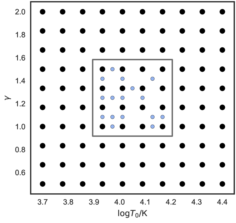
Figure 1: Grid of thermal parameters applied to a DM only simulation at $z=2$ used to construct a model of the $b$-$N_{\text{HI}}$ distribution. The black points show the combinations of $\log T_{0}$ and $\gamma$ imposed onto our simulation (“standard grid”). The square marks the area that will be used for inference tests. The blue points indicate where further models were generated for testing the robustness of the method presented in this work (“test grid”).

The corresponding flux skewer $F$, i.e. a transmission spectrum along the line-of-sight, is calculated from the optical depth using $F=\exp(-A_{r}\,\tau)$. Here we introduce a scaling factor $A_{r}$ that allows us to match our lines-of-sight to observed mean flux values $\bar{F}$. The mean flux normalization is computed for the full snapshot, i.e. the factor $A_{r}$ is iteratively changed until the mean flux of the snapshot converges to a desired (measured) mean flux. We apply that value of $A_{r}$ to all the spectra when generating skewers, so there is one mean flux normalization of the whole box and sightline to sightline variations are still present in our models. This re-scaling of the optical depth accounts for our lack of knowledge of the precise value of the metagalactic ionizing background photoionization rate and it is done simply to generate more realistic skewers. To this end we choose $A_{r}$ so that we agree with the effective opacity $\tau_{\text{eff}}=-\ln(\bar{F})$ at $z=2$ from Faucher-Giguère et al. (2008b), namely $\tau_{\text{eff}}=0.127$.

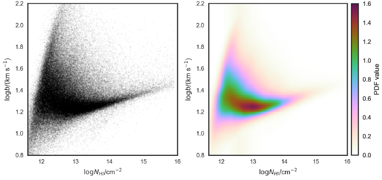
Figure 2: Left: A $b$-$N_{\text{HI}}$ distribution illustrated as a cloud of points generated by concatenating the VPFIT output for 6000 skewers from a DM only simulation snapshot at $z=2$ with thermal parameters $(\log T_{0},\gamma)=(4.011,1.333)$. This distribution consists of $\sim 1.5\times 10^{5}$ absorbers. Right: The KDE based PDF of the same distribution (as described in § 3.1).

2.1 Thermal Parameter Grid

Using our simulation snapshot at $z=2$ we generated 6000 skewers for each of 100 combinations of thermal parameters $\log T_{0}$ and $\gamma$ at a fixed $\lambda_{P}=73.3\,$\mathrm{kpc}$$. Figure 1 shows the distribution of thermal parameters chosen (black points). We chose to model the thermal parameters on a 10$\times$10 regular grid covering the range $3.7\leq\log(T_{0}/\text{K})\leq 4.4$ and $0.5\leq\gamma\leq 2.0$, which is dense enough to sample typical uncertainties in $T_{0}$ and $\gamma$. The number of skewers at each grid point was chosen, so that we have enough absorbers to ensure that our estimation of the shape of the $b$-$N_{\text{HI}}$ distribution is converged. This is important, as we will use the absorbers in the $b$-$N_{\text{HI}}$ distribution to estimate $P(\log N_{\text{HI}},\log b\>|\>\log T_{0},\gamma)$ which we will introduce in § 3.1. In this work we will refer to this grid as the “standard grid”.

In addition, we generated 16 models between the grid points in the central region of our grid (region marked with the square and blue points in Figure 1). These were randomly chosen from a regular grid twice as fine as the standard grid, excluding the points that coincide with it. These additional models will be used in § 3.3 to test the robustness of our procedure for generating model $b$-$N_{\text{HI}}$ distributions, as well as our statistical inference (see § 4.2). We will refer to these extra models as the “test grid”.

2.2 Forward Modeling Noise and Resolution

The technique presented in the following section is based on the sensitivity of the shape of the $b$-$N_{\text{HI}}$ distribution on the thermal state of the IGM. Therefore, it is important that instrumental effects which can also affect the shape of the $b$-$N_{\text{HI}}$ distribution, such as noise and spectroscopic resolution, are properly included into the models we wish to compare to data.

To mimic instrumental resolution we convolve the skewers with a Gaussian with FWHM = 6 $\mathrm{km}\text{\,}{\mathrm{s}}^{-1}$, which is the typical resolution delivered by echelle spectrometers (see e.g. the High Resolution Echelle Spectrometer (HIRES) (Vogt et al. 1994; Lehner et al. 2014; O’Meara et al. 2016, 2017) and Ultraviolet and Visual Echelle Spectrograph (UVES) (Dekker et al. 2000; Dall’Aglio et al. 2008) dataset in Hiss et al. 2018). Further, we add Gaussian random noise to the skewers assuming a fixed signal-to-noise ratio (SNR) of 63 per resolution element for the purpose of choosing a value comparable to the SNR of the dataset in Hiss et al. (2018) at $z=2$.

We apply the exact same Voigt-profile fitting scheme described in Hiss et al. (2018) to the 6000 forward modeled simulated skewers generated for 100 different combinations of $T_{0}$, $\gamma$. To summarize, Voigt-profiles were fitted to our simulated data using VPFIT version 10.2 (Carswell & Webb 2014). We wrote a fully automated set of wrapper routines that prepare the spectra for the fitting procedure and controls VPFIT with the help of the VPFIT front-end/back-end programs RDGEN and AUTOVPIN.

VPFIT decomposes segments of spectra into a set of Voigt-profiles characterized by 3 parameters each: line redshift $z_{\text{abs}}$, Doppler parameter $b$, and column density $N_{\text{HI}}$ for the Hydrogen Ly$\alpha$ transition. We set up VPFIT to explore the range of parameters $1\leq b/$\mathrm{km}\text{\,}{\mathrm{s}}^{-1}$\leq 300$ and $11.5\leq\log(N_{\text{HI}}{}/\text{\text{cm}${}^{-2}${}})\leq 16$ when fitting absorption profiles. We chose to fit in this $N_{\text{HI}}$ range in order encompass typical optically thin Ly$\alpha$ absorbers ranging from low column densities (where most of lines are comparable to noise) to very rare high column densities. Concerning the Doppler parameter, the chosen fitting region ranges from narrow absorbers, that are unphysical and have broadening comparable to the UVES/HIRES resolution element, to broad absorbers that are substantially broader than the typical absorber around the cutoff for all $\log T_{0}$ and $\gamma$ combinations in our grid. This choice of fitting range is appropriate, as the probability of encountering absorbers close to the edge of our fitting range drops to nearly zero at this redshift.

VPFIT finds the best fit by varying the profile parameters and searching for a solution that minimizes the $\chi^{2}$. If the $\chi^{2}$ is not satisfying, then further absorption components are added until the fit converges or no longer improves. We take into account that VPFIT often has difficulty fitting the boundaries of spectra by artificially increasing the length of the sightlines. For this purpose we append the first (last) quarter of the spectra to the end (beginning) of it, therefore making the spectra longer by 50%. This manipulation does not cause discontinuities in the flux, as the simulation box is periodic. We later ignore absorbers within the artificially enlarged areas.

Additionally, in order to avoid using badly constrained absorber parameters, we exclude points that have relative uncertainties worse than 50% in $b$ or $N_{\text{HI}}$. These lines are rejected in order to remove absorbers that are badly constrained. As discussed in Rudie et al. (2012) and Hiss et al. (2018), most of these lines arise in blended and noisy regions. Additionally, as the $\log$ errors are proportional to the relative errors, we expect a 50% relative error to be $\text{d}\log x=\ln(10)\cdot\text{d}x/x=\ln(10)\cdot 0.5\simeq 1.15$ (x being either $N_{\text{HI}}$ or $b$). These uncertainties are substantially larger than our kernel density estimation bandwidth used in this study (see § 3.1) which additionally motivated us to to exclude these absorbers. Finally, filtering these lines consistently in data and models should not bias our results, as these are mostly VPFIT artifacts and will consistently arise whenever there is noise and blending.

For every combination of $\log T_{0}$ and $\gamma$, a $b$-$N_{\text{HI}}$ distribution can be generated from all absorbers found for all skewers. One example with $(\log T_{0},\gamma)=(4.011,1.333)$ is shown in the left panel of Figure 2.

3 Method for Emulating the Full $b$-$N_{\text{HI}}$ Distribution

In this section, we introduce the method used to generate PDFs of $b$-$N_{\text{HI}}$ distributions at any location in thermal parameter space based on our grid of simulated thermal models. For each thermal model, we perform Kernel Density Estimation (KDE) to determine $P(\log N_{\text{HI}},\log b)$ from the discrete absorbers identified by VPFIT. To interpolate the $b$-$N_{\text{HI}}$ distribution between points in our parameter grid we modified the emulation technique of Heitmann et al. (2006) and Habib et al. (2007), initially developed for power spectrum analysis, to our purpose. Note that this approach has also been used in the context of measurements of the evolution of the thermal state of the IGM in Rorai et al. (2013b, 2017) and Walther et al. (2018b).

We apply principal component analysis (PCA) to decompose this set of probability distribution maps onto a set of basis vectors, yielding a set of coefficients $\Theta_{j}(T_{0},\gamma)$ for each thermal model corresponding to principal component vectors $\boldsymbol{e}_{j}$. We then use Gaussian process (GP) interpolation to evaluate these coefficients at arbitrary locations in parameter space, which combined with the basis vectors, results in a model for $P(\log N_{\text{HI}},\log b\>|\>\log T_{0},\gamma)$.

Finally, we present a Bayesian method for determining the posterior distribution of thermal parameters from an observed set of $\log N_{\text{HI}}$ and $\log b$. We refer to this procedure of model construction and inference, based on PCA decomposition of KDE estimates of a PDF, as the PKP method. The details of each step are discussed in what follows.

3.1 Kernel density estimation of the $b$-$N_{\text{HI}}$ distribution PDF

In the first step of the PKP approach we use KDE to construct the probability density distribution from which points in the $b$-$N_{\text{HI}}$ distributions of our models were drawn. This is achieved by treating each data point $\{\log N_{\rm{HI},i},\log b_{i}\}$ as a smooth kernel centered at the measurements position $\log N_{\rm{HI},i}$ and $\log b_{i}$. We use a Gaussian kernel of the form

$$K_{i} (\sigma_{\log N_{\text{HI}}},\sigma_{\log b})=\frac{1}{2\pi\sigma_{\log N_{\rm{HI}}}\sigma_{\log b}}\times$$ (3)

$$\exp\left({-\frac{1}{2}\left[\frac{(\log N_{\rm{HI}}-\log N_{\rm{HI},i})^{2}}{\sigma_{\log N_{\rm{HI}}}^{2}}+\frac{(\log b-\log b_{i})^{2}}{\sigma_{\log b}^{2}}\right]}\right),$$

characterized by a bandwidth $(\sigma_{\log N_{\text{HI}}},\sigma_{\log b})$ that regulates how much one wishes to smooth a measurement in each dimension. Note that the Kernel used in eqn. 3 assumes no correlation between $\log N_{\rm{HI},i}$ and $\log b_{i}$ for a given pair. This assumption should not significantly affect the estimated PDFs, because the single Kernels overlap substantially.

With every measurement described as a smooth distribution, we can generate an estimate for the probability density function from which a set of measurements $\{\log N_{\rm{HI},j},\log b_{j}\}$ with $j=1,...,N$, was drawn

$$P(\log N_{\rm{HI}},\log b)=\frac{1}{N}\sum_{j=1}^{N}K_{j}(\sigma_{\log N_{\text{HI}}},\sigma_{\log b}).$$ (4)

In other words, we compute $P(\log N_{\text{HI}},\log b)$ by replacing each measurement with a Gaussian kernel with a constant bandwidth, summing them up and normalizing the distribution.

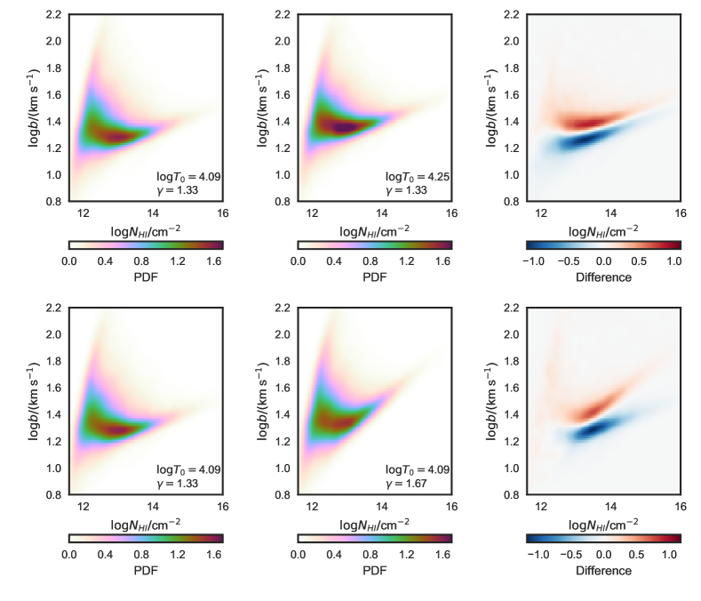
Figure 3: Sensitivity of $P(\log N_{\text{HI}},\log b)$ on the thermal parameters imposed onto our simulation. Left: $P(\log N_{\text{HI}},\log b)$ based on the KDE of $b$-$N_{\text{HI}}$ distributions at a given point in our thermal grid. Middle: $P(\log N_{\text{HI}},\log b)$ based on the KDE of $b$-$N_{\text{HI}}$ distributions at a given point in our thermal grid choosing higher $\log T_{0}$ (upper panel) and higher $\gamma$ (lower panel). Right: The difference between the distributions illustrates that increasing $\log T_{0}$ shifts $P(\log N_{\text{HI}},\log b)$ toward higher $b$ (top), while increasing $\gamma$ mainly tilts the distribution at $\log(N_{\text{HI}}$/cm^-2)$>13$ (bottom).

In this study, we compute KDEs using the package KDEMultivariate from the statsmodels python module (Seabold & Perktold 2010). An example of this method applied to one of our $b$-$N_{\text{HI}}$ distributions is shown in the right panel of Figure 2 for one particular combination of thermal parameters $(\log T_{0},\gamma)=(4.011,1.333)$, which can be compared to the points in the $b$-$N_{\text{HI}}$ distribution determined by VPFIT in the left panel.

We generate KDE based $P(\log N_{\text{HI}},\log b)$ for every thermal parameter combination in our standard thermal grid by applying KDE to the points in the $b$-$N_{\text{HI}}$ distribution determined by VPFIT, using a bandwidth of $(\sigma_{\log N_{\rm HI}},\sigma_{\log b})=(0.08,0.032)$ for each dimension. We tuned our bandwidth using mock datasets in order avoid oversmoothing of $P(\log N_{\text{HI}},\log b\>|\>\log T_{0},\gamma)$, which can wash out structure in the distribution. Additionally, oversmoothing shifts the peak of $P(\log N_{\text{HI}},\log b\>|\>\log T_{0},\gamma)$ towards high $b$ due to the asymmetry of the distribution, resulting in a distribution that has its maximum clearly shifted from the highest concentration of absorbers in the cloud of points used to generate it. At the same time we were careful not to undersmooth the distribution, which leads to a noisy PDF.

For comparison, a Silverman estimation of the optimal bandwidth (Silverman 1986) for our dataset, which assumes that the underlying distribution is Gaussian, typically yields a bandwidth of $(0.1,0.04)$. This choice resulted in a very slight bias in our measurements for mock data in the context of the inference test described in § 4.2, indicating that this choice of bandwidth oversmoothes our distributions.

To illustrate the sensitivity of our PDF to thermal parameters we show $P(\log N_{\text{HI}},\log b\>|\>\log T_{0},\gamma)$ for different $\log T_{0}$ and $\gamma$ combinations in Figure 3. We observe that, as expected, most of the sensitivity of the $b$-$N_{\text{HI}}$ distribution with respect to the parameters of the TDR lies in its lower $b$ envelope. Therefore, in the limit of a measurement of $T_{0}$ and $\gamma$, our approach can be interpreted as an alternative way of retrieving the cutoff (although without many of the problems associated with iterative cutoff fitting as described in § 1). Nevertheless, our method can be expanded to any changes in the general form of the $b$-$N_{\text{HI}}$ distribution, provided that these are properly modeled in the simulations. The example of $T_{0}$ and $\gamma$ is an interesting starting point to apply our method to, but should not be seen as its sole application. We know for instance that $\lambda_{P}$ (Garzilli et al. 2015, 2018), the fraction of the gas in the warm-hot phase (Danforth et al. 2016) and galactic feedback (Viel et al. 2017) affect the shape of the $b$-$N_{\text{HI}}$ distribution above the location of the cutoff. In principle, our method should be sensitive to these parameters as well.

For better intuition about the thermal sensitivity of the $b$-$N_{\text{HI}}$ distribution we also added Figures, constructed from the output of hydrodynamical simulations described in § 5.1, to appendix A. These can be be viewed as animations in the HTML version of this manuscript (available in the refereed version only).

3.2 Decomposition of the PDF into Principal Components

Given the non-parametric nature of KDE, there is no direct way to generate $P(\log N_{\text{HI}},\log b\>|\>\log T_{0},\gamma)$ for combinations of $\log T_{0}$ and $\gamma$ between points in our thermal grid positions. For this to be possible, we have to parametrize the $P(\log N_{\text{HI}},\log b\>|\>\log T_{0},\gamma)$ maps. To this end, we evaluate the KDE of each $b$-$N_{\text{HI}}$ distribution on a $100\times 100$ mesh in the $b$-$N_{\rm HI}$ plane and then decompose these pixelized PDFs onto a set of linear independent principal components, thus parametrizing the KDE based $P(\log N_{\text{HI}},\log b\>|\>\log T_{0},\gamma)$ with PCA coefficients and a set of basis vectors.

Specifically, we discretized the PDFs in the region $11.5\leq\log(N_{\text{HI}}/\text{\text{cm}${}^{-2}$})\leq 16.$ and $0.8\leq\log(b/$\mathrm{km}\text{\,}{\mathrm{s}}^{-1}$)\leq 2.2$), adopting a pixel size $(0.04,0.014)$ in $(\log N_{\text{HI}},\log b)$, which is a factor of 2 smaller than the bandwidth chosen for the KDE. Then we compute the (natural) logarithm of the probabilities at every pixel. Given our small pixels, we expect no significant change in the shape of the $b$-$N_{\text{HI}}$ distribution due to pixelization. All examples of smooth $b$-$N_{\text{HI}}$ distributions shown in this work are pixelized on this grid (see e.g. Figures 2, 3, and 5).

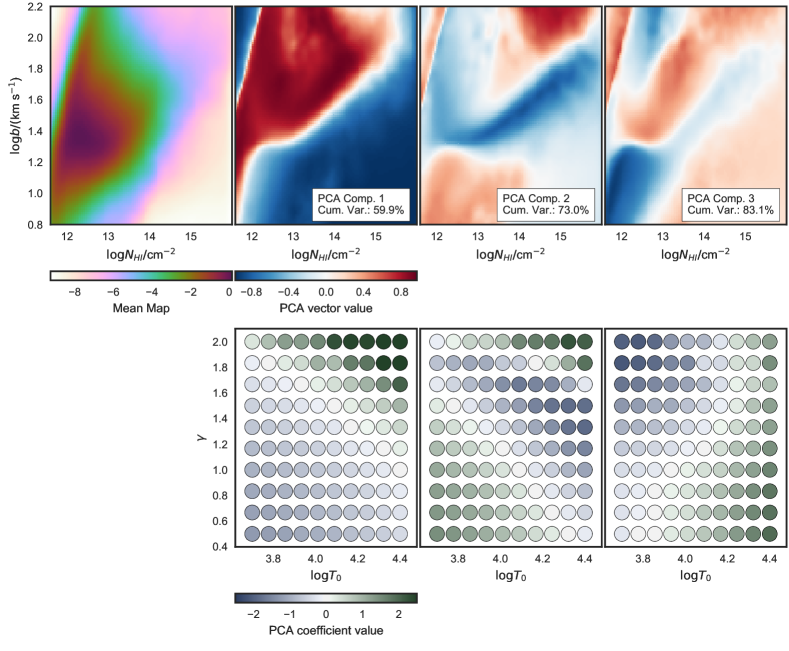
Figure 4: Upper row: The mean map $\boldsymbol{\mu}(\log N_{\text{HI}}$, $\log b$) and the first 3 principal component vectors $\boldsymbol{e}_{j}$ from our principal component analysis of our model maps. Note that the decomposition was carried out in the natural logarithm of the probability. The vectors were reshaped to the map form of $100\times 100$ pixels and are sorted by contribution to the cumulative variance (see text for details). Lower row: The corresponding principal component coefficients $\Theta_{j}(\log T_{0},\gamma)$ for each map.

The PCA is performed by decomposing our discrete maps into a basis of principal component vectors $\boldsymbol{e}_{j}$, which makes it possible to recover any model in our grid by linearly combining the principal component vectors, using the coefficients $\Theta_{j}(\log T_{0},\gamma)$ and adding them to the mean map $\boldsymbol{\mu}(N_{\text{HI}},b)$:

$$\ln P(\log N_{\text{HI}},\log b\>|\>\log T_{0},\gamma)=\boldsymbol{\mu}(\log N_{\text{HI}},\log b)$$ (5)

$$+\sum_{j=1}^{N}\Theta_{j}(\log T_{0},\gamma)\boldsymbol{e}_{j}(\log N_{\text{HI}},\log b),$$

where $N$ is the number of models available, in this case $N=100$, and the components are ranked by their contribution to the cumulative variance of the dataset. In short, the PCA decomposes a matrix of all vectorized $\ln$$P(\log N_{\text{HI}},\log b)$ maps into a basis of 100 principal component vectors with 100 coefficients each.

In Figure 4 we show the $\boldsymbol{\mu}(\log N_{\text{HI}},\log b)$ map and the first 3 principal component vectors (reshaped to an image of 100$\times$100 pixels) and coefficients from our analysis. Note that PCA is a standard method for dimensionality reduction, as it allows one to choose the principal components that encompass most of the variance within the data by ignoring components that do not contribute substantially to the cumulative variance. The cumulative contribution to the total variance is computed by first dividing the eigenvalues from the singular value decomposition method used in the PCA by their sum, ordering them in descending order, and computing their cumulative sum. For illustration, the first 3 components shown in Figure 4 already account for 83.1% of the cumulative variance in the models. At present, we are not interested in dimensionality reduction and keeping all 100 PCA components is not computationally prohibitive for the current case. By PCA decomposing the KDEs in our grid, we are simply describing each of the discretized $P(\log N_{\text{HI}},\log b\>|\>\log T_{0},\gamma)$ with a set of coefficients $\Theta_{j}(T_{0},\gamma)$ and basis vectors, enabling a parametric description of $P(\log N_{\text{HI}},\log b\>|\>\log T_{0},\gamma)$.

There are two reasons why we carried out the PCA on $\ln$$P(\log N_{\text{HI}},\log b)$. First, because we will interpolate PCA components of $\ln P(\log N_{\text{HI}},\log b\>|\>\log T_{0},\gamma)$ maps (§ 3.3) in thermal parameter space, and these PDFs have sharp features (such as the low $b$ cutoff). Computing the natural logarithm is desirable to reduce interpolation errors. Second, we do this for a practical reason, as we will ultimately tie this analysis to a Markov Chain Monte Carlo (MCMC) algorithm that works with the $\log$-likelihood.

The disadvantage of working with the natural logarithm of $P(\log N_{\text{HI}},\log b\>|\>\log T_{0},\gamma)$ is that the probability fluctuations around zero are amplified, which can destabilize the interpolation process in the low probability regions. To avoid interpolation artifacts in the low probability regime, we simply apply a probability threshold to all our discrete $\ln P(\log N_{\text{HI}},\log b\>|\>\log T_{0},\gamma)$ maps under which all probabilities are set to zero. We chose to set this threshold at the value of the 20th percentile of the probability values for each map. Typically this threshold corresponds to a probability $<0.003$, i.e. it only affects the lowest probabilities of $P(\log N_{\text{HI}},\log b\>|\>\log T_{0},\gamma)$ and doesn’t vary strongly from model to model. Varying this threshold did not affect our emulated distributions substantially for values lower than the 40th percentile of the probability values for each map, as the cut involves the lowest probability regions.

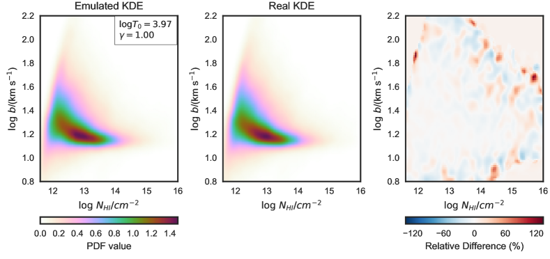
Figure 5: Comparison of interpolated and measured $P(\log N_{\text{HI}},\log b\>|\>\log T_{0},\gamma)$ for a model in our test grid, i.e. not included in the grid used for constructing the $\ln P(\log N_{\text{HI}},\log b\>|\>\log T_{0},\gamma)$ emulator. Thermal parameters are $(\log T_{0},\gamma)=(3.972,1.0)$. Left: $P(\log N_{\text{HI}},\log b\>|\>\log T_{0},\gamma)$ constructed by interpolating PCA components using GP interpolation. Middle: $P(\log N_{\text{HI}},\log b\>|\>\log T_{0},\gamma)$ generated from KDE of the PDF directly from the VPFIT output at the same thermal parameters. Right: The difference of emulated and original $b$-$N_{\text{HI}}$ distribution relative to the original $b$-$N_{\text{HI}}$ distribution illustrates that we are able to accurately emulate the PDF between our grid points. The fact that we see no relative difference in the edges of the rightmost diagram comes from the fact that we set a density threshold under which the probability was set to zero (see § 3.2).

3.3 Emulating the PDF

Finally, we train a Gaussian process on the PCA coefficients for our discrete model grid (using GEORGE Ambikasaran et al. 2016). This allows us to generate $\ln$$P(\log N_{\text{HI}},\log b)$ at arbitrary $\log T_{0}$ and $\gamma$ combinations.

A Gaussian process is basically a stochastic process for which every finite subset of random variables is normally distributed, i.e. it can be fully described by its mean and a covariance function. The covariance function is a measure of how much two points in parameter space $\boldsymbol{\vartheta}_{l}$ and $\boldsymbol{\vartheta}_{m}$ are covariant, $\boldsymbol{\vartheta}$ being a vector with $(\log T_{0},\gamma)$ in our parameter-space. We adopt a standard choice for the covariance $C$, which is a squared-exponential kernel plus an additional white noise contribution, with the form:

$$C(\boldsymbol{\vartheta}_{l},\boldsymbol{\vartheta}_{m})=\exp\left(-0.5\,(\boldsymbol{\vartheta_{l}}-\boldsymbol{\vartheta_{m}})\,C_{h}^{-1}\,(\boldsymbol{\vartheta_{l}}-\boldsymbol{\vartheta_{m}})\right)+\sigma_{n}\delta_{\mathrm{lm}},$$ (6)

where $C_{h}$ is chosen to be a diagonal matrix with a smoothing length $h_{l}$ for every dimension, i.e. the characteristic distance beyond which the covariance between two points drops, and $\sigma_{n}$ parametrizes the white noise term. We chose $h_{l}$ to be a constant with the value of 20% of our standard thermal grid length in each dimension (larger than the typical grid separation). This guarantees that the interpolation will correlate coefficients $\Theta_{j}(T_{0,i},\gamma_{i})$ from neighboring points in the grid.

There is an infinite number of functions that satisfy a Gaussian process with a specific mean and covariance, but the interpolation (or regression) part comes in once we only select the subset of functions that are constrained to pass through a particular set of points. In our case, we have a vector of 100 PCA coefficients $\Theta_{j}(T_{0,i},\gamma_{i})$ for each model combination $i$ in our grid of 100 simulations. Although GP interpolation can be generalized for the case in which the computed PCA coefficients have uncertainties by having the white noise term $\sigma_{n}\delta_{\mathrm{ij}}$ in eqn. 6, we decided to assume that these PCA coefficients have no uncertainty, i.e. we force the interpolation to pass nearly perfectly through the measured $\Theta_{j}(T_{0,i},\gamma_{i})$ by setting $\sigma_{n}$ to nearly zero. This means that our emulator essentially recovers the $b$-$N_{\text{HI}}$ distribution maps perfectly at the thermal grid positions.

We illustrate the accuracy of our procedure in Figure 5. In the left panel we show an emulated $P(\log N_{\text{HI}},\log b\>|\>\log T_{0},\gamma)$ for a $(\log T_{0},\gamma)$ = $(3.972,1.0)$ combination between points in our standard grid. The middle panel shows the true KDE based PDF from the VPFIT output for this thermal model (taken from our test grid). The right panel shows the relative difference between the two PDFs, which scatters around 0 and is typically of the order of 3% in probability in the high probability regions, indicating that we can successfully interpolate between models. The difference drops to zero in the far edges due to the thresholding of the density described in § 3.2. There are some peaks in the relative difference close to the edges, that arise simply because the 20th percentile density thresholding did not affect the exact same pixels in the real vs. the emulated distribution.

We will further discuss the effect of the GP interpolation when performing mock measurements in § 4.2.

3.4 Parameter Inference

We use the $\ln P(\log N_{\text{HI}},\log b\>|\>\log T_{0},\gamma)$ emulator as a basis for calculating the likelihood of a dataset given model parameters. The probability of measuring a single absorption line $(N_{\text{HI},i},b_{i})$ is given by the PDF $P(\log N_{\text{HI}},\log b\>|\>\log T_{0},\gamma)$. Thus the likelihood for measuring a set of $N$ absorption lines ${\log N_{\rm HI},\log b}$ is

$$\mathscr{L}=\displaystyle\prod^{N}_{i}P(\log N_{\text{HI},i},\log b_{i}\>|\>\log T_{0},\gamma),$$ (7)

or in terms of log-likelihood

$$\ln\mathscr{L}=\sum_{i}^{N}\ln P(\log N_{\text{HI},i},\log b_{i}\>|\>\log T_{0},\gamma).$$ (8)

Given that our emulator is able to generate model PDFs at any given point within the thermal parameter grid, we simply couple this log-likelihood to a MCMC algorithm to perform Bayesian inference of the model parameters. For this purpose we use the python package emcee (Foreman-Mackey et al. 2013) which implements the affine invariant sampling technique (Goodman & Weare 2010). We assumed flat priors for both parameters which are truncated at the edges of our standard thermal grid for all MCMC runs presented in this paper.

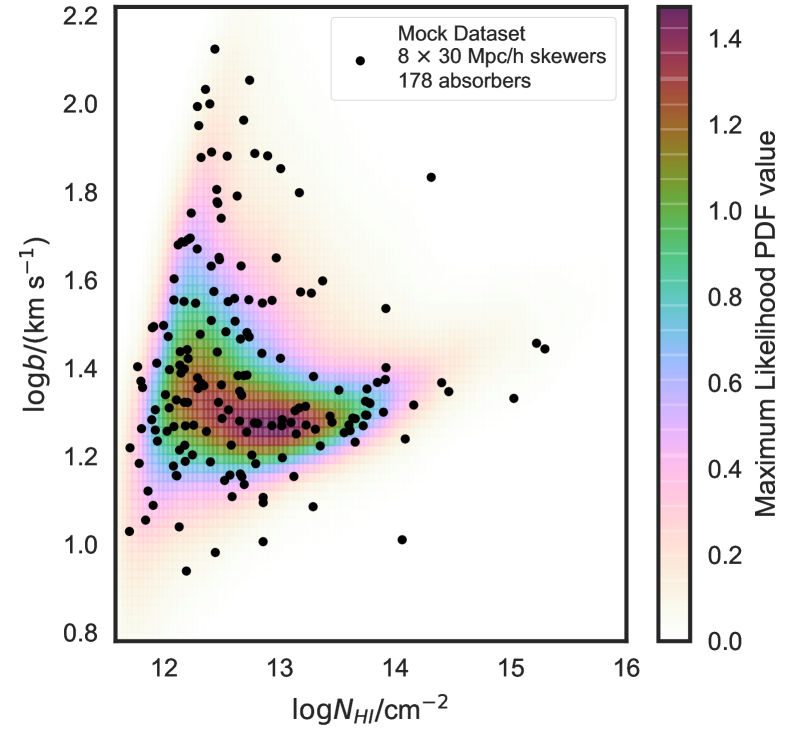
Figure 6: A mock realization of a data $b$-$N_{\text{HI}}$ distribution composed of the absorbers from eight randomly chosen skewers from a simulation with $(\log T_{0},\gamma)=(4.050,1.333)$. An emulated $P(\log N_{\text{HI}},\log b\>|\>\log T_{0},\gamma)$ based on the median values of the marginal distributions of the corresponding MCMC posterior ($\log T_{0}=4.054$ and $\gamma=1.303$, see Figure 7) is shown for comparison.

The key assumption of the likelihood above is that we treat the Ly$\alpha$ forest as being an uncorrelated distribution of lines such that we can look upon each $\log N_{\text{HI}},\leavevmode\nobreak\ \log b$ measurement as a random draw from $P(\log N_{\text{HI}},\log b\>|\>\log T_{0},\gamma)$. We expect that this assumption does not affect our likelihood substantially given the low level of spatial correlations in the Ly-a forest (McDonald et al. 2006). We will carry out an inference test in § 4.2 and asses if this affects mock measurements carried out with the PKP method.

4 Testing the Robustness of our Inference

In this section we test the PKP method by carrying out mock measurements of $\log T_{0}$ and $\gamma$ using MCMC. First we show one example of a measurement and then we test the robustness of our method by examining how the MCMC posteriors behave for measurements based on many random realizations of mock datasets for the models in our test grid.

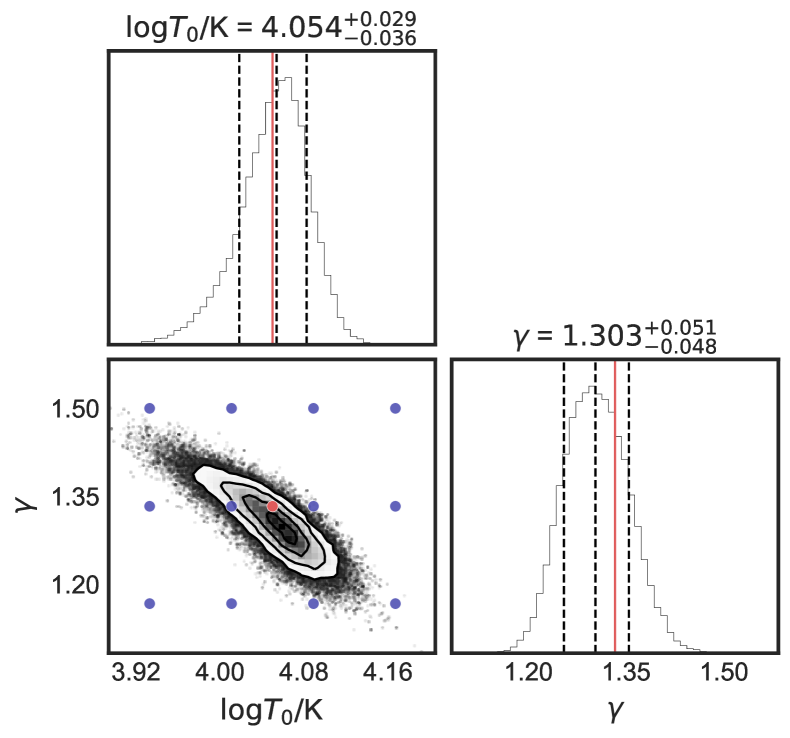
Figure 7: MCMC posterior for a mock dataset composed of eight randomly chosen skewers (absorbers shown in Figure 6) extracted from a model in our test grid with thermal parameters shown in red. A zoomed in part of the thermal grid used for constructing the emulator on which this measurement is based is shown in blue. The model from which the mock data were chosen (red dot) is not included when constructing the $\ln P(\log N_{\text{HI}},\log b\>|\>\log T_{0},\gamma)$ emulator.

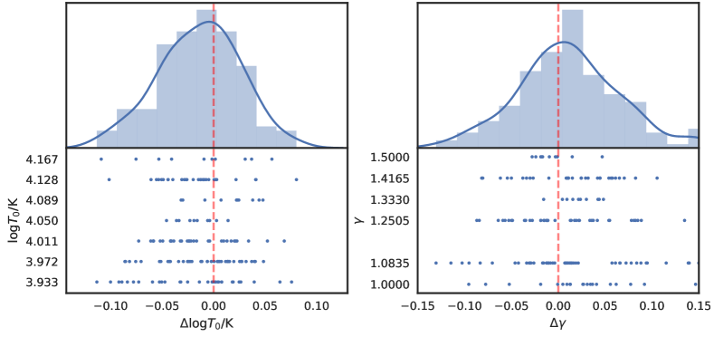
Figure 8: Distribution of the difference between the true values and the medians of MCMC posteriors for 10 random realizations of mock datasets with eight skewers each for all the 16 test models (blue in Figure 1). The likelihoods for these measurements were calculated based on $P(\log N_{\text{HI}},\log b\>|\>\log T_{0},\gamma)$ generated using our emulator, which did not include these models. The differences between true values and MCMC based estimates are shown as blue points in the lower panels for each realization. A histogram of all measurements put together is shown in blue, while the blue line corresponds to a 1D KDE of the differences in the histogram. The red dashed line illustrates a perfect measurement.

4.1 Measurement Example

As an example of a mock measurement we select the absorbers from a sample of eight random skewers extracted from a model with $(\log T_{0},\gamma)=(4.050,1.333)$ in our test grid (the blue points in Figure 1). The corresponding dataset is shown as black points in Figure 6. For reference, this mock dataset is comparable in terms of pathlength to the redshift range 1.9 to 2.1 provided by a single quasar spectrum in the Hiss et al. (2018) analysis. Specifically, this dataset is generated from a pathlength of $240$\mathrm{Mpc}$$. While a single Ly$\alpha$ forest at this redshift (between Ly$\alpha$ and Ly$\beta$ emission peaks) covers $\sim 620$\mathrm{Mpc}$$ (from $z=2.1$ to 1.7). In Hiss et al. (2018) the redshift bin used was 1.9 to 2.1, so each quasar spectrum contributed $\sim 295$\mathrm{Mpc}$$. Effectively, due to the masking applied to the data in order to filter possible metal contaminants and the pathlength reduction associated with it, our mock dataset corresponds to nearly two sightlines in terms of number of absorbers at this redshift range.

The results of our MCMC inference for this particular mock dataset are shown in Figure 7. We observe the well known strong degeneracy in the measurement of $\log T_{0}$ and $\gamma$, which is a result from setting the pivot-point of the TDR at mean density (see e.g. Lidz et al. 2010; Becker et al. 2011; Walther et al. 2018b; Hiss et al. 2018). We obtain $\log T_{0}=4.054^{+0.029}_{-0.036}$ and $\gamma=1.303^{+0.051}_{-0.048}$, whereby the errors are calculated based on the 16th and 84th percentiles of the marginalized distributions of the MCMC posterior. One observes that this is remarkably close to the true model that the dataset was drawn from (indicated by the red dot and lines in Figure 7). We can illustrate the inferred model PDF by inputting these measured thermal parameters (i.e. the median of the individual marginalized posteriors) into into our emulator, retrieving the corresponding $\ln P(\log N_{\text{HI}},\log b\>|\>\log T_{0},\gamma)$ and computing $\exp($$\ln P(\log N_{\text{HI}},\log b\>|\>\log T_{0},\gamma)$), which is shown by the color coded distribution in Figure 6.

4.2 Inference Test

In order to further test the robustness of our method, we perform measurements of $\log T_{0}$ and $\gamma$ using 10 mock data realizations of $b$-$N_{\text{HI}}$ distributions (based on eight random skewers each) for each of the 16 models in the test grid. Our uncertainties are quantified based on the two dimensional MCMC posteriors (see e.g. Figure 7). Testing our measurements by inspecting many realizations of mock datasets will reveal if our method is returning valid posterior probability distributions.

Given that we are dealing with models exactly between our standard grid points, this test will show if interpolation errors in $\ln P(\log N_{\text{HI}},\log b\>|\>\log T_{0},\gamma)$ result in biased measurements. This is a crucial test given that our typical MCMC contours have uncertainties that are comparable to the characteristic separation between models in our thermal grid, which is illustrated by the blue grid points shown in Figure 7. Furthermore, an inference test will fail, for instance, if our assumption that we can neglect spatial correlations in the Ly$\alpha$ forest in the likelihood in eqn. 8 is incorrect.

We test if the uncertainties derived from the MCMC posteriors are sensible by carrying out the following exercise. For all of the 160 posteriors, i.e. 16 distinct models times 10 mock realizations of each model, we quantify how often the true values of the thermal parameters used land within the 68% and 95% confidence regions of the corresponding 2D MCMC posterior. We observe that the true values are within the 68% confidence region 68.7% (110/160) of the time, and that they are within the 95% confidence region 96.9% (155/160) of the time. This convincingly indicates that our posterior distributions are robust and that we are not over or underestimating our uncertainties.

As a further test of whether our inference is significantly biased, we examine the distribution of the difference between the true values of $\log T_{0}$ and $\gamma$ and the median of the marginalized distributions of the MCMC posteriors: $\Delta\log T_{0}=\log T_{0,\text{true}}-\log T_{0,\text{MCMC}}$ and $\Delta\gamma=\gamma_{\text{true}}-\gamma_{\text{MCMC}}$. The distributions of these differences are presented in Figure 8. We see that the distributions are centered around zero, indicating that any bias associated with our method is smaller than the resulting uncertainties. Note that in this initial experiment we are deliberately only carrying out our tests for the measurement of $T_{0}$ and $\gamma$, not taking into account the correlations with other parameters such as pressure smoothing scale $\lambda_{p}$ or amplitude of the UVB. While certainly important, adding these dimensions to our analysis is beyond the scope of introducing and testing our new approach.

5 Pilot Study: A Measurement of Thermal Parameters at z=2

The DM only models used for our inference test in § 4.2 use an approximation for generating flux skewers which does not capture the full physical picture necessary to properly represent the IGM (Sorini et al. 2016). While DM only simulations were sufficient for our initial tests (see § 2), for a realistic measurement involving real observational data, one has to use hydrodynamical simulations to generate model distributions. In this section we apply the PKP method to real Ly$\alpha$ forest absorption line data using a grid of hydrodynamical simulations to model $P(\log N_{\text{HI}},\log b\>|\>\log T_{0},\gamma)$.

5.1 The $P(\log N_{\text{HI}},\log b\>|\>\log T_{0},\gamma)$ from Hydrodynamical Simulations

Following the approach described in § 2 and 3, we now generate models of $P(\log N_{\text{HI}},\log b\>|\>\log T_{0},\gamma)$ by applying VPFIT to simulated skewers drawn from hydrodynamical simulations of different thermal models. Hydrodynamic simulations provide the general physical conditions that give rise to the Ly$\alpha$ forest directly from first principles, with exception of reionization effects, thus resulting in realistic $b$-$N_{\text{HI}}$ distributions. Additionally, pressure smoothing of absorbers is accounted for in a physical way as opposed to the artificial smoothing of the density field that was used in the DM models. The disadvantage associated with hydrodynamical simulations is that, unlike the DM based model, it is costly to generate large grids in $T_{0}$ and $\gamma$ at a given redshift, which could pose a problem given the high precision our method can achieve. Nevertheless, grids of $\sim 30$ hydrodynamical simulations are computationally feasible (see below).

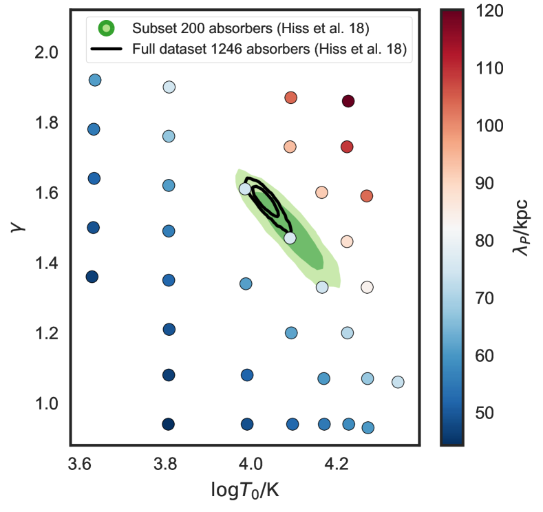
Figure 9: Thermal grid from snapshots of hydrodynamical simulations from the THERMAL suite at $z=2$ used in this pilot study. The points are colored based on the pressure smoothing scale $\lambda_{P}$. For comparison with the characteristic grid separation, we show the measurements (see § 5.3) achieved using the full dataset from Hiss et al. (2018) (black contour lines) and a subset of 200 absorbers from this dataset (green contours).

For the purpose of generating a basis of model $b$-$N_{\text{HI}}$ distributions, we use part of the publicly available THERMAL suite of Nyx simulations (Almgren et al. 2013; Lukić et al. 2015) presented in Hiss et al. (2018). The THERMAL suite consists of more than 60 Nyx hydrodynamical simulations with different thermal histories and $L_{\text{box}}=20\,\text{Mpc}/h$ and $1024^{3}$ cells based on a Planck Collaboration et al. (2014) cosmology $\Omega_{m}=0.3192$, $\Omega_{\Lambda}=0.6808$, $\Omega_{b}=0.04964$, $h=0.6704$, $n_{s}=0.96$, $\sigma_{8}=0.826$. We chose a grid consisting of a subset of 36 simulation snapshots at $z=2$ with different combinations of $T_{0}$, $\gamma$ and $\lambda_{P}$ that result from different thermal evolutions (Oñorbe et al. 2017), shown in Figure 9.

Note that, although arbitrary $\lambda_{P}$ values could be generated in principle, it would require substantial computing power to fine-tune the reionization histories to do so. As discussed in Walther et al. (2018b), it is difficult to generate physically realistic models without correlating the TDR parameters and $\lambda_{P}$, because the pressure smoothing scale depends on the integrated thermal history of the IGM. Due to computing time restrictions, we generate only physically motivated $\lambda_{P}$ which are correlated with the TDR parameters, i.e. high (low) $T_{0}$ and $\gamma$ combinations generate large (small) values of $\lambda_{P}$.

Following our discussion in § 3.1, we apply the same KDE procedure to the VPFIT output of our simulations and then construct a $\ln P(\log N_{\text{HI}},\log b\>|\>\log T_{0},\gamma)$ emulator based on simulated $b$-$N_{\text{HI}}$ distributions (as in § 3.3). For the $\ln P(\log N_{\text{HI}},\log b\>|\>\log T_{0},\gamma)$ emulation we apply the same PCA and GP interpolation scheme, adopting smoothing lengths $h$ in the covariance (see eqn. 6) for the interpolator that is 50% of the grid size in the $\log T_{0}$ direction and 20% in $\gamma$ direction. Additionally, for the white noise term in eqn. 6 we chose $\sigma_{n}=0.01$, which allows for small deviations in the interpolation at the grid points. These changes relative to the DM only emulation were arrived at via visual inspection of the emulated PDFs. Specifically, we changed these parameters until no interpolation artifacts were present throughout the grid. A motivation of this choice of white noise contribution is presented in the appendix B.2. Additionally, similar to the analysis of mock datasets in § 4.2, we checked if we accurately recover the thermal parameters at the grid positions and found that the results were unbiased. This indicates that the different Gaussian process smoothing parameters and white noise term added when using hydrodynamic simulations do not significantly bias our inference.

5.2 Absorption Line Dataset

In order to carry out a measurement, we use the absorption line data from Hiss et al. (2018) which consists of 1246 absorption lines at $1.9\leq z<2.1$.

One problem that could bias the results of our method are outliers with low $b$ in the $b$-$N_{\text{HI}}$ distribution. Hiss et al. (2018) argued that these are narrow lines added by VPFIT in order to decrease the $\chi^{2}$ of the fit in blended absorption features, and unidentified metal absorbers wrongly assumed to be Ly$\alpha$ lines (as observed by Schaye et al. (1999); Rudie et al. (2012)). Blending artifacts should not have a severe impact on our measurements, as a proper forward modeling of the simulated sightlines should include the same sort of contamination in our model $P(\log N_{\text{HI}},\log b\>|\>\log T_{0},\gamma)$.

As for dealing with metal line contamination, the dataset used was carefully masked for metal absorption systems, as described in Hiss et al. (2018); Walther et al. (2018a). The severity of metal line contamination is strongly redshift dependent, as the identification of metal absorbers in the Ly$\alpha$ forest becomes increasingly difficult at higher redshift (and nearly unfeasible at $z\gtrsim 3.5$) due to line blanketing as the effective optical depth of the Ly$\alpha$ forest increases. In our case, the contamination should be relatively mild, given that metal line absorbers are more easily identified at lower redshifts and that these data were previously masked for potential contaminants using different automatic and interactive techniques. Nevertheless there are remaining unidentified contaminants, that have to be excluded with some sort of outlier rejection.

In Hiss et al. (2018) they implemented an iterative 2$\sigma$ rejection procedure based on Rudie et al. (2012) that rejects potential narrow line contaminants in the range $12.5<\log N_{\text{HI}}/\text{\text{cm}${}^{-2}$}<14.5$. For simplicity, we decided to extrapolate the 2$\sigma$ rejection line defined in Hiss et al. (2018) to the region $11.5<\log N_{\text{HI}}/\text{\text{cm}${}^{-2}$}<16$ (shown as a gray dashed line in Figure 10) and discard all absorbers with $\log b$ lower than this line. Alternatively, one could implement a more elegant outlier modeling method such as the one used by Telikova et al. (2018), but here we opt for this simpler approach.

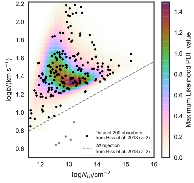
Figure 10: A subset of the $b$-$N_{\text{HI}}$ distribution from Hiss et al. (2018) composed of 200 randomly chosen absorbers (black points). To avoid possible narrow line contaminants (gray points) only absorbers with $b$ above the extrapolated 2$\sigma$ rejection line from Hiss et al. (2018) were chosen (gray dashed line). An emulated $P(\log N_{\text{HI}},\log b\>|\>\log T_{0},\gamma)$ based on the median values of the marginal distributions of the corresponding MCMC posterior is shown for comparison.

The dataset from Hiss et al. (2018) has a size of 1246 absorbers, and we have intuition from § 4.2 that this dataset size would result in percent level precision, i.e. smaller than the spacing between our thermal grid points, making our inference susceptible to interpolation uncertainties. We thus decided to randomly choose a set of 200 absorbers from this dataset, hence with a similar number of lines as the mock dataset of eight skewers described in § 4. In contrast to the SNR modeling done in § 2.2 using a constant value of 63 per 6 $\mathrm{km}\text{\,}{\mathrm{s}}^{-1}$, we randomly chose the SNR from the real sightlines for the mock spectra from hydrodynamical simulations to better represent the noise distribution within the data (exactly as was done in Hiss et al. 2018). Because of this approach, it makes more sense to chose a random subset of absorbers rather than selecting a random subset of quasar sightlines. For a discussion about how our results differ if we randomly choose QSO sightlines instead of absorbers please refer to the appendix C.

To understand how our uncertainties compare to the typical separations between points in our thermal parameter grid we show two sets of $\log T_{0}$-$\gamma$ measurements in Figure 9. We will explain in detail how these contours were measured in the next section. But for the sake of the current discussion, note that the green contours result from analyzing a dataset of 200 absorbers, resulting a precision comparable to our characteristic grid separation; whereas, the black contours show a measurement using the complete dataset of 1246 absorbers. Clearly, using the full dataset results in an uncertainty substantially smaller than our grid spacing, which indicates that interpolation errors could be a significant issue. Given the exquisite precision delivered by the PKP method and the size of existing datasets, it is challenging to generate a grid of hydro simulations fine enough to do justice to the implied precision. Nevertheless, we believe that this is computationally within reach and will enable measurements of the thermal state of the IGM with unprecedented precision.

5.3 Results

In order to measure $\log T_{0}$ and $\gamma$, we carry out the same Bayesian measurement as described in § 4, this time using real data combined with $P(\log N_{\text{HI}},\log b)$ emulated from hydrodynamical simulations. The subset of 200 absorbers from Hiss et al. (2018) are shown as black points in Figure 10, whereas the five gray points are the corresponding fraction of absorbers that are rejected. The green contours in Figure 9 shows the MCMC posterior resulting from analyzing these data, from which we measure $\log T_{0}=4.092^{+0.050}_{-0.055}$ and $\gamma=1.49^{+0.073}_{-0.074}$, whereby the errors are calculated based on the 16th and 84th percentiles of the marginalized distributions. We explore how this inference behaves for different random realizations of 200 absorbers in the appendix C. As before, we emulate the $P(\log N_{\text{HI}},\log b\>|\>\log T_{0},\gamma)$ at these measured values which is shown as the color coded distribution in Figure 10.

Additionally, we carried out the same measurement using the full dataset of 1264 lines from Hiss et al. (2018). As discussed in § 5.2, due to the current separations in our model grid, we have concerns about interpolation error at such a high level of precision. Nevertheless, we wanted to illustrate the kind of precision achievable using existing data. With these caveats, we measure $\log T_{0}=4.034^{+0.022}_{-0.019}$ and $\gamma=1.576^{+0.026}_{-0.032}$. The corresponding contours are shown in black in Figure 9. Importantly, compared to the measurement using a subset of these data, the uncertainties are smaller by a factor of approximately $\sqrt{6}$, which is the expected scaling due to the relative sizes of the datasets.

5.3.1 Comparison with Cutoff Fitting Results

These PKP based results can be compared to the Hiss et al. (2018) measurements from the same dataset using the cutoff fitting approach. From the marginalized distributions of the Hiss et al. (2018) Monte Carlo based posteriors, they measured $\log T_{0}=4.137^{+0.050}_{-0.074}$ and $\gamma=1.47^{+0.12}_{-0.10}$ at $z=2$ using the 1264 Ly$\alpha$ absorbers.

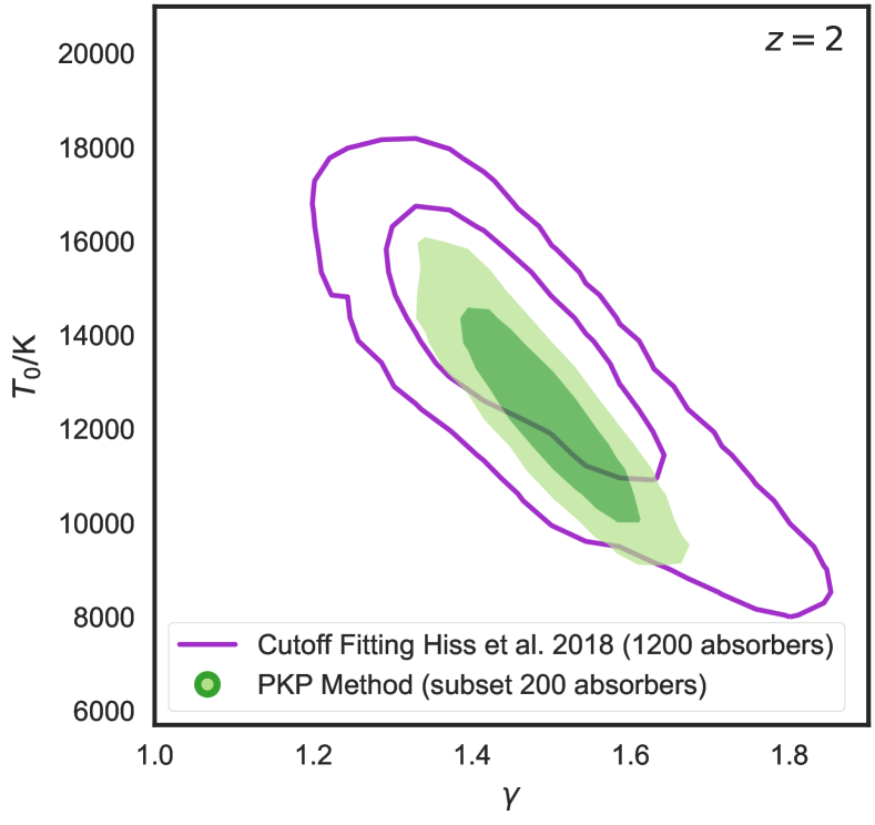
Figure 11: Comparison of the thermal parameter constraints from Hiss et al. (2018) using the cutoff fitting method (purple contour lines), and our measurement using the PKP method (green contours). While the original dataset from Hiss et al. (2018) has a size of $1246$ absorbers, only 845 are actually used for cutoff fitting due to the fact that only absorbers with $12.5\leq\log(N_{\text{HI}}{}/\text{\text{cm}${}^{-2}${}})\leq 14.5$ and $8<b/$\mathrm{km}\text{\,}{\mathrm{s}}^{-1}$<100$ are used. The cutoff fitting results are shown as purple contour lines. When using the PKP method described in this study, we achieve higher precision (green contours) while using a random subset of 200 absorbers from their data.

As stated in § 5.3, when applying our new method to a subset of 200 absorbers from their dataset, we measure $\log T_{0}=4.092^{+0.050}_{-0.055}$ and $\gamma=1.49^{+0.073}_{-0.074}$. In Figure 11 we compare our PKP based measurement using just 200 absorbers from Hiss et al. (2018) (green shaded contours) to the cutoff fitting measurement from Hiss et al. (2018) using the full dataset (purple contours).

A direct comparison of these measurements based on the size of the dataset used is challenging, because both methods use different cuts in the data. While we use all absorbers within the allowed fitting range, the cutoff fitting method only uses the absorbers within $12.5\leq\log(N_{\text{HI}}{}/\text{\text{cm}${}^{-2}${}})\leq 14.5$ and $8<b/$\mathrm{km}\text{\,}{\mathrm{s}}^{-1}$<100$. In Hiss et al. (2018) this reduces the initial dataset of 1264 to 845 absorbers which are effectively used for cutoff fitting.

As described in § 5.3, using the complete dataset results in a dramatic improvement in the precision compared to Hiss et al. (2018). This improvement comes from the fact that the constraining power of the cutoff method depends only weakly on the number of absorbers in the $b$-$N_{\text{HI}}$ distribution, as discussed in detail by Schaye et al. (1999) (see their Figure 14), and hence its precision does not scale as $\sqrt{N}$ as one would naively expect. In contrast, the advantage of the PKP method is that it delivers a precision which scales approximately as $\sqrt{N}$, delivering higher precision for larger datasets.

For a more direct comparison one can calculate what uncertainties we would expect for a dataset of 845 absorbers, i.e. the exact number of absorbers effectively used for cutoff fitting. Under the assumption of $\sqrt{N}$ scaling, our representative uncertainties for a dataset of 200 absorbers, for example $\sigma_{\log T_{0}}=0.055$ and $\sigma_{\gamma}=0.074$, become smaller by a factor $\sqrt{845/200}$, i.e $\sigma_{\log T_{0}}=0.027$ and $\sigma_{\gamma}=0.036$. In this case our result would be around factor of two in $\log T_{0}$ and a factor of nearly three in $\gamma$ more precise than cutoff fitting for 845 absorbers.

Indeed, the main limitation in PKP precision, which we have already encountered for the current dataset, is the number of simulations required to generate a model grid dense enough to deliver the implied precision. However, we believe this is a surmountable problem given currently available computational resources.

Finally, we note that another complication associated with the cutoff fitting method is that one has to adopt a value of the column density $N_{\text{HI},0}$ that corresponds to the mean density in order to relate the minimal Doppler parameter at this density $b_{0}=b_{min}(N_{\text{HI},0})$ to $T_{0}$. With this new approach we circumvent this issue, as we are sensitive to the shape of the $b$-$N_{\text{HI}}$ distribution at all column densities. Furthermore, Hiss et al. (2018) showed that cutoff fitting is sensitive to the details of the iterative cutoff fitting method (least squares or mean deviation minimization), which can lead to differences in the results. In contrast, the Bayesian likelihood (eqn. 8) that provides the underpinnings of PKP does not require that one make these somewhat arbitrary choices.

6 Discussion and Summary

In this work we introduced a new method for inferring thermal parameters from the $b$-$N_{\text{HI}}$ distribution of Ly$\alpha$ forest absorbers in the IGM, the PKP method. In contrast to a large body of previous work focused on analyzing a small subset of lines to fit the lower cutoff of the $b$-$N_{\text{HI}}$ distribution, our new approach utilizes all available data and exploits parameter sensitivity encoded in the full shape of this distribution. We generated a large grid of simulations of the Ly$\alpha$ forest encompassing a range of different thermal parameter models, and fit the resulting mock spectra with VPFIT, generating a large database of absorption lines for each model. Our new method applies KDE to sets of discrete absorption lines to generate model $b$-$N_{\text{HI}}$ distribution PDFs, then uses a PCA decomposition to create an emulator for this distribution which can be evaluated at any location in thermal parameter space. Using this emulator, we introduced a Bayesian likelihood formalism enabling parameter inference via MCMC. We conducted a pilot study demonstrating the efficacy of this new approach in the limit of a two dimensional $T_{0}$ and $\gamma$ measurement, whereby real observational data at $z=2$ was compared to a grid of hydrodynamical simulations. The primary results of this work are:

1. Using 160 mock measurements we demonstrated that our statistical inference procedure delivers unbiased estimates of thermal parameters and reports valid uncertainties.

2. Our new method was applied to real observational data to measure the parameters of the TDR at $z=2$. We found $\log T_{0}=4.092^{+0.050}_{-0.055}$ and $\gamma=1.49^{+0.073}_{-0.074}$ using just a subset 200 absorbers from the dataset of Hiss et al. (2018), which roughly corresponds, in terms of pathlength, to a single Ly$\alpha$ forest spectrum at $z\simeq 2$.

3. For current dataset sizes at $z$=$2$, the PKP method can already deliver a precision on $\log T_{0}$ ($\gamma$) nearly two (three) times higher than the cutoff fitting method.

In the future this method could be expanded to include other parameters that affect the shape of the $b$-$N_{\text{HI}}$ distribution. One could model different thermal histories by including the pressure scale $\lambda_{P}$ as a free parameter, allow the mean flux $\bar{F}$ to vary, which would constrain the UVB, or analyze IGM models with additional physics such as blazar heating (Puchwein et al. 2012; Sironi & Giannios 2014; Lamberts et al. 2015) or galaxy formation feedback (Sorini et al. 2018). Our new methodology is readily applicable to the $z>2$ Ly$\alpha$ forest, as shown by our pilot study at $z=2$, as well as to existing Hubble Space Telescope Cosmic Origins Spectrograph (HST/COS) ultraviolet (UV) spectra (e.g. Danforth et al. 2013, 2016) that probes the Ly$\alpha$ forest at $z\lesssim 0.5$. Indeed, measuring the thermal state of the IGM at these low redshifts with high precision could help clarify the nature of the discrepancy of the $b$-$N_{\text{HI}}$ distribution between observations and hydrodynamical simulations that have been recently highlighted (Viel et al. 2017; Gaikwad et al. 2017; Nasir et al. 2017).

Appendix A Thermal Sensitivity Animations

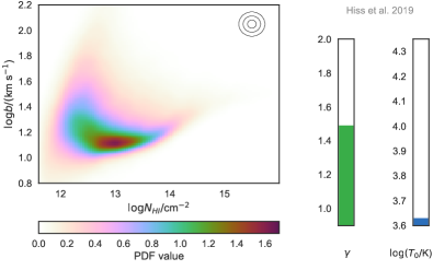
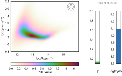
Figure 12: These Figures are meant to be viewed as animations in the HTML version of this manuscript (available in the refereed version only). Both animations were generated using our emulator based on hydrodynamical simulations described in § 5.1. Left: Change of the shape of the $b$-$N_{\text{HI}}$ distribution when changing $\log T_{0}$ from 3.63 to 4.26 in ten equal steps at a fixed $\gamma=1.49$. Similar to the effect illustrated in the upper panels of Figure 3, increasing $\log T_{0}$ shifts the distribution toward higher $b$. Right: Change of the shape of the $b$-$N_{\text{HI}}$ distribution when changing $\gamma$ from 0.94, 1.87 in ten equal steps at a fixed $\log T_{0}=4.09$. Similar to the effect illustrated in the lower panels of Figure 3, increasing $\gamma$ mainly tilts the distribution at $\log(N_{\text{HI}}$/cm^-2)$>13$. For both panels, the concentric rings on the top right represents the KDE bandwidth chosen (1, 2, and 3$\sigma$). Note that there is a change in the pressure smoothing scale included in these animations which is not explicitly shown. As shown in Figure 9, this particular emulator was built based on a grid that correlates the thermal parameters and the pressure smoothing scale due to the dependence of $\lambda_{P}$ on the integrated thermal history of the IGM. Broadening across this characteristic length is responsible for the turn over in the distribution visible at $\log(N_{\text{HI}}$/cm^-2)$<13$ when increasing either $\log T_{0}$ or $\gamma$.

Appendix B Choice of Emulation Hyperparameters

B.1 Emulator Smoothing Length $h_{l}$

To motivate the choice of $h_{l}=0.2$ for our emulator smoothing length for the DM only models, we compare the true PDF for a model with $\log T_{0}=4.128$ and $\gamma=1.4165$ to the emulated PDF at the same thermal parameters using different smoothing lengths in Figure 13. This particular model is not included in the emulator building process, but is part of our test grid (see Figure 1), and was chosen to lie as far away from grid points as possible. We show the true PDF, i.e. the one computed directly from the $b$-$N_{\text{HI}}$ distribution, in the upper left panel and the difference between emulated and real PDF for different $h_{l}$ in the other panels. Essentially, the emulated PDF differs substantially from the true one when choosing very small (smaller than grid separation, i.e. emulator does not correlate neighboring models) and very large $h_{l}$ ($>$factor of 3 grid separation). The emulator shows a stable performance in the intermediate range $0.03\leq h_{l}\leq 0.3$ which implies that the choice of $h_{l}=0.2$ is adequate. Note that this example shows the worst case scenario where the emulated PDF is the farthest away from the grid points and the interpolation has the highest uncertainty.

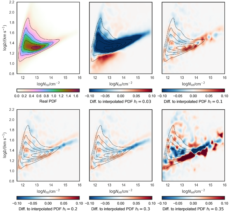
Figure 13: The difference between true and emulated maps for a model with $\log T_{0}=4.128$ and $\gamma=1.4165$ (not included in the DM only emulation grid and maximally far away from points in the grid). The emulated PDFs were constructed from emulators using different smoothing lengths. Using a smoothing length that is too small results in an interpolation that does not take into account close grid points, while a large smoothing length introduces artifacts. We observe small fluctuations in comparison with the true PDF for intermediate $0.03<h_{l}<0.3$ for our DM only emulation scheme.

B.2 White Noise Contribution $\sigma_{n}$

In § 5.1 we state that we chose the value $\sigma_{n}=0.01$ for the hydrodynamic simulation grid based on visual inspection, because we observed clear interpolation artifacts in a few places inside the thermal grid when adopting no white noise contribution. To explore the effect of this choice, we show in Figure 14 one example with $\log T_{0}=3.9$ and $\gamma=1.19$ that generated such artifacts. The upper left panel shows the color coded map and contours for the choice used in this study. All other panels represent different choices of white noise contribution. Note that this choice of $\log T_{0}$ and $\gamma$ represents the worst case of artifacts we encountered within the grid, and it corresponds to a location where the interpolation covers a substantial gap in parameter space. Unfortunately, we do not have the option of generating extra models as we did with the DM only simulations, i.e. the true PDF at this grid position is unknown, but Figure 14 indicates that (in this worst case scenario) the general shape of the emulated $b$-$N_{\text{HI}}$ distribution does not present artifacts for $\sigma_{n}>0.005$ and keeps its general shape until $\sigma_{n}$ is large ($>0.1$) and the interpolation has so much freedom in the grid points that the shape of the $b$-$N_{\text{HI}}$ distribution loses information about the thermal state of the gas.

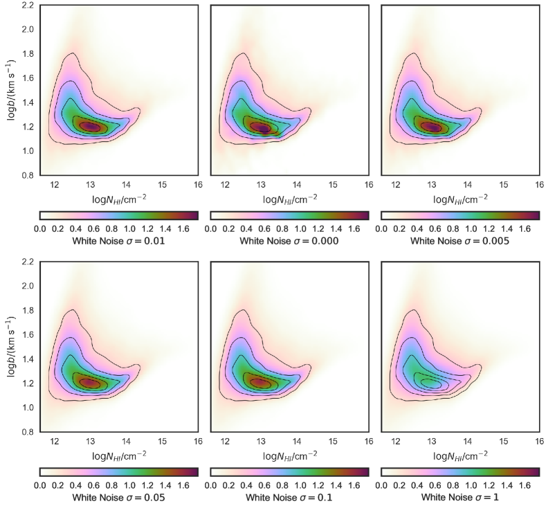
Figure 14: Emulated $b$-$N_{\text{HI}}$ distribution for $\log T_{0}=3.9$ and $\gamma=1.19$ using the hydrodynamic grid for different values of the white noise term $\sigma_{n}$. The emulated PDF resulting from an emulation using our fiducial choice of $\sigma_{n}=0.01$ is shown in the upper left panel as a color coded map and corresponding contours. All other panels show the $b$-$N_{\text{HI}}$ distribution, but emulated using different white noise contributions. The contours of our fiducial choice are shown for comparison in all panels. This figure illustrates that allowing no freedom for the interpolation at the grid points results in interpolation artifacts in this particular position (between grid points). Additionally, allowing too much freedom results in loss of information about the thermal state.

Appendix C Effect of Different Data Subsampling Methods

As stated in § 5.2, we chose to draw 200 absorbers randomly from the dataset of Hiss et al. (2018), because the models used to construct the $b$-$N_{\text{HI}}$ distribution PDFs have a mixed SNR with a distribution based on our data. This approach could pose a problem, as random picking across the full dataset essentially removes correlations between absorbers in the same spectra. We showed in section 4.2, using DM only simulations, that our inference is robust in the case of a fixed SNR and mock datasets composed of 8 randomly drawn skewers, i.e. correlations are included and the SNR does not affect our inference test. To understand if these effects play a role in the measurement presented in § 5.3, one should investigate the effects of picking random QSO sightlines instead of random absorbers, given that our likelihood is agnostic to correlations between absorption lines. In the following paragraphs we will explore both approaches.

To test if our inference is influenced by randomly choosing absorbers, we generated another 200 realizations of 200 randomly chosen absorbers from the full dataset and carried out the same inference as in § 4.1. Note that, while the same absorbers are present in different realizations, absorbers are picked without replacement such that the same absorbers does not appear more than once in each individual realization. As a measure for how consistent the measurements of all these realizations are with each other, given that we do not know the true value, we compare the measurements of each realization to the measurement using the full dataset presented in § 5.3. We observe that the measurements from the full dataset ($\log T_{0}=4.034$ and $\gamma=1.576$) are within the 1$\sigma$ contour of the 2D posteriors of these realizations 65% (129/200) of the time, and within the 2$\sigma$ contour of the 2D posterior 96% (192/200) of the time. This implies that our inference is consistent in the limit of random realizations based on absorbers. For illustration, the posteriors for six realizations are shown in Figure 15. For reference we also plot the measurement from the full dataset as a black dot.

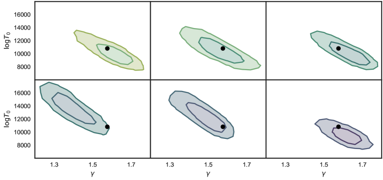
Figure 15: The 1 and 2$\sigma$ contours for 6 measurement realizations (out of 200), each consisting of 200 unique randomly chosen absorbers from the dataset of Hiss et al. (2018) at $z=2$. The black dot illustrates the median of the measurements using the full dataset.

We ran a similar test, this time choosing random QSO sightlines instead of random absorbers. Due to metal line masking, at $z=2$ each QSO in our sample contributes with $\sim 100$ absorbers, which means that we would carry out a measurement using around 2 sightlines each time (see discussion in § 4.1). To test if we achieve results that are consistent with the full dataset, we carried out this experiment using 11 quasars that span or nearly span the pathlength within $1.9<z<2.1$, which results in 55 unique pairs of quasars and therefore measurement realizations. We observe that the reference values measured using the full dataset are within the 1$\sigma$ contours of the 2D MCMC posteriors of these realizations about 33% (18/55) of the time. This implies that there is some bias associated with choosing QSO sightlines randomly instead of absorbers. Note that we do not have sufficient statistics to quantify the behavior of the 95% contours with a sample size of 55 realizations.

One possible reason for failing this inference test when choosing the pairs of QSO sightlines is the fact that we are choosing non-representative SNR values by picking random QSOs and comparing their $b$-$N_{\text{HI}}$ distributions to models that were constructed to match the SNR distribution of the whole dataset. The proper approach to remove a possible SNR bias would be to generate a set of models with the matching SNR for each data subsample separately, i.e. generate a set of forward-models for every quasar pair in the example above. This approach would require applying VPFIT to our full model grid and recreating a $b$-$N_{\text{HI}}$ distribution emulator for every MCMC posterior we wish to generate. We have considered this approach, but concluded it implies a significant computational effort, given that the current calculations are already extremely resource consuming when done once. Additionally, real physical sightline to sightline variations in the TDR, could also perform the poor performance on this inference test. If present these variations would mean that subsampling by choosing random absorbers essentially results in a measurement of the average TDR in that specific sub sample.

References

- Almgren et al. (2013) Almgren, A. S., Bell, J. B., Lijewski, M. J., Lukić, Z., & Van Andel, E. 2013, ApJ, 765, 39
- Ambikasaran et al. (2016) Ambikasaran, S., Foreman-Mackey, D., Greengard, L., Hogg, D. W., & O’Neil, M. 2016, TPAMI, 38, 252
- Becker et al. (2011) Becker, G. D., Bolton, J. S., Haehnelt, M. G., & Sargent, W. L. W. 2011, MNRAS, 410, 1096
- Boera et al. (2018) Boera, E., Becker, G. D., Bolton, J. S., & Nasir, F. 2018, ArXiv e-prints, arXiv:1809.06980
- Boera et al. (2014) Boera, E., Murphy, M. T., Becker, G. D., & Bolton, J. S. 2014, MNRAS, 441, 1916
- Bolton et al. (2014) Bolton, J. S., Becker, G. D., Haehnelt, M. G., & Viel, M. 2014, MNRAS, 438, 2499
- Bolton et al. (2008) Bolton, J. S., Viel, M., Kim, T.-S., Haehnelt, M. G., & Carswell, R. F. 2008, MNRAS, 386, 1131
- Carswell & Webb (2014) Carswell, R. F., & Webb, J. K. 2014, VPFIT: Voigt profile fitting program, Astrophysics Source Code Library, ascl:1408.015
- Compostella et al. (2013) Compostella, M., Cantalupo, S., & Porciani, C. 2013, MNRAS, 435, 3169
- Compostella et al. (2014) —. 2014, MNRAS, 445, 4186
- Croft et al. (1998) Croft, R. A. C., Weinberg, D. H., Katz, N., & Hernquist, L. 1998, ApJ, 495, 44
- Dall’Aglio et al. (2008) Dall’Aglio, A., Wisotzki, L., & Worseck, G. 2008, AAP, 491, 465
- Danforth et al. (2013) Danforth, C., Pieri, M., Shull, J. M., et al. 2013, in American Astronomical Society Meeting Abstracts, Vol. 221, American Astronomical Society Meeting Abstracts #221, 245.04
- Danforth et al. (2016) Danforth, C. W., Keeney, B. A., Tilton, E. M., et al. 2016, ApJ, 817, 111
- Dekker et al. (2000) Dekker, H., D’Odorico, S., Kaufer, A., Delabre, B., & Kotzlowski, H. 2000, in Society of Photo-Optical Instrumentation Engineers (SPIE) Conference Series, Vol. 4008, Optical and IR Telescope Instrumentation and Detectors, ed. M. Iye & A. F. Moorwood, 534–545
- Dixon & Furlanetto (2009) Dixon, K. L., & Furlanetto, S. R. 2009, ApJ, 706, 970
- Dixon et al. (2014) Dixon, K. L., Furlanetto, S. R., & Mesinger, A. 2014, MNRAS, 440, 987
- Faucher-Giguère et al. (2008a) Faucher-Giguère, C.-A., Lidz, A., Hernquist, L., & Zaldarriaga, M. 2008a, ApJ, 688, 85
- Faucher-Giguère et al. (2008b) Faucher-Giguère, C.-A., Prochaska, J. X., Lidz, A., Hernquist, L., & Zaldarriaga, M. 2008b, ApJ, 681, 831
- Foreman-Mackey et al. (2013) Foreman-Mackey, D., Hogg, D. W., Lang, D., & Goodman, J. 2013, PASP, 125, 306
- Gaikwad et al. (2017) Gaikwad, P., Srianand, R., Choudhury, T. R., & Khaire, V. 2017, MNRAS, 467, 3172
- Garzilli et al. (2012) Garzilli, A., Bolton, J. S., Kim, T.-S., Leach, S., & Viel, M. 2012, MNRAS, 424, 1723
- Garzilli et al. (2015) Garzilli, A., Theuns, T., & Schaye, J. 2015, MNRAS, 450, 1465
- Garzilli et al. (2018) —. 2018, ArXiv e-prints, arXiv:1808.06646
- Gnedin & Hui (1996) Gnedin, N. Y., & Hui, L. 1996, ApJL, 472, L73
- Gnedin & Hui (1998a) —. 1998a, MNRAS, 296, 44
- Gnedin & Hui (1998b) —. 1998b, MNRAS, 296, 44
- Goodman & Weare (2010) Goodman, J., & Weare, J. 2010, CAMCoS, 5, 65
- Gunn & Peterson (1965) Gunn, J. E., & Peterson, B. A. 1965, ApJ, 142, 1633
- Habib et al. (2007) Habib, S., Heitmann, K., Higdon, D., Nakhleh, C., & Williams, B. 2007, Phys. Rev. D, 76, arXiv:astro-ph/0702348
- Heitmann et al. (2006) Heitmann, K., Higdon, D., Nakhleh, C., & Habib, S. 2006, ApJ, 646, L1
- Hiss et al. (2018) Hiss, H., Walther, M., Hennawi, J. F., et al. 2018, ApJ, 865, 42
- Hui & Gnedin (1997) Hui, L., & Gnedin, N. Y. 1997, MNRAS, 292, 27
- Khaire et al. (2016) Khaire, V., Srianand, R., Choudhury, T. R., & Gaikwad, P. 2016, MNRAS, 457, 4051
- Khaire et al. (2018) Khaire, V., Walther, M., Hennawi, J. F., et al. 2018, ArXiv e-prints, arXiv:1808.05605
- Kulkarni et al. (2015) Kulkarni, G., Hennawi, J. F., Oñorbe, J., Rorai, A., & Springel, V. 2015, Apj, 812, 30
- Kulkarni et al. (2018) Kulkarni, G., Worseck, G., & Hennawi, J. F. 2018, ArXiv e-prints, arXiv:1807.09774
- Lamberts et al. (2015) Lamberts, A., Chang, P., Pfrommer, C., et al. 2015, ArXiv e-prints, arXiv:1502.07980
- Lee et al. (2015) Lee, K.-G., Hennawi, J. F., Spergel, D. N., et al. 2015, ApJ, 799, 196
- Lehner et al. (2014) Lehner, N., O’Meara, J. M., Fox, A. J., et al. 2014, ApJ, 788, 119
- Lidz et al. (2010) Lidz, A., Faucher-Giguère, C.-A., Dall’Aglio, A., et al. 2010, ApJ, 718, 199
- Lukić et al. (2015) Lukić, Z., Stark, C. W., Nugent, P., et al. 2015, MNRAS, 446, 3697
- Lynds (1971) Lynds, R. 1971, Apj, 164, L73
- Madau & Haardt (2015) Madau, P., & Haardt, F. 2015, ApJL, 813, L8
- Madau & Meiksin (1994) Madau, P., & Meiksin, A. 1994, ApJ, 433, L53
- McDonald et al. (2001) McDonald, P., Miralda-Escudé, J., Rauch, M., et al. 2001, ApJ, 562, 52
- McDonald et al. (2006) McDonald, P., Seljak, U., Burles, S., et al. 2006, ApJS, 163, 80
- McGreer et al. (2015) McGreer, I. D., Mesinger, A., & D’Odorico, V. 2015, MNRAS, 447, 499
- McQuinn et al. (2009) McQuinn, M., Lidz, A., Zaldarriaga, M., et al. 2009, Apj, 694, 842
- McQuinn & Upton Sanderbeck (2016) McQuinn, M., & Upton Sanderbeck, P. R. 2016, MNRAS, 456, 47
- Meiksin & White (2001) Meiksin, A., & White, M. 2001, MNRAS, 324, 141
- Miralda-Escudé et al. (2000) Miralda-Escudé, J., Haehnelt, M., & Rees, M. J. 2000, ApJ, 530, 1
- Nasir et al. (2017) Nasir, F., Bolton, J. S., Viel, M., et al. 2017, MNRAS, 471, 1056
- Oñorbe et al. (2017) Oñorbe, J., Hennawi, J. F., & Lukić, Z. 2017, ApJ, 837, 106
- O’Meara et al. (2017) O’Meara, J. M., Lehner, N., Howk, J. C., et al. 2017, ArXiv e-prints, arXiv:1707.07905
- O’Meara et al. (2016) —. 2016, VizieR Online Data Catalog, 515
- Peeples et al. (2010) Peeples, M. S., Weinberg, D. H., Davé, R., Fardal, M. A., & Katz, N. 2010, MNRAS, 404, 1295
- Planck Collaboration et al. (2014) Planck Collaboration, Ade, P. A. R., Aghanim, N., et al. 2014, AAP, 571, A16
- Puchwein et al. (2012) Puchwein, E., Pfrommer, C., Springel, V., Broderick, A. E., & Chang, P. 2012, MNRAS, 423, 149
- Ricotti et al. (2000) Ricotti, M., Gnedin, N. Y., & Shull, J. M. 2000, ApJ, 534, 41
- Robertson et al. (2015) Robertson, B. E., Ellis, R. S., Furlanetto, S. R., & Dunlop, J. S. 2015, ApJL, 802, L19
- Rorai et al. (2018) Rorai, A., Carswell, R. F., Haehnelt, M. G., et al. 2018, MNRAS, 474, 2871
- Rorai et al. (2013a) Rorai, A., Hennawi, J. F., & White, M. 2013a, ApJ, 775, 81
- Rorai et al. (2013b) —. 2013b, ApJ, 775, 81
- Rorai et al. (2017) Rorai, A., Hennawi, J. F., Oñorbe, J., et al. 2017, Science, 356, 418
- Rudie et al. (2012) Rudie, G. C., Steidel, C. C., & Pettini, M. 2012, ApJ, 757, L30
- Schaye (2001) Schaye, J. 2001, Apj, 559, 507
- Schaye et al. (1999) Schaye, J., Theuns, T., Leonard, A., & Efstathiou, G. 1999, MNRAS, 310, 57
- Schaye et al. (2000) Schaye, J., Theuns, T., Rauch, M., Efstathiou, G., & Sargent, W. L. W. 2000, MNRAS, 318, 817
- Seabold & Perktold (2010) Seabold, S., & Perktold, J. 2010, in 9th Python in Science Conference
- Silverman (1986) Silverman, B. W. 1986, Density estimation for statistics and data analysis
- Sironi & Giannios (2014) Sironi, L., & Giannios, D. 2014, ApJ, 787, 49
- Sorini et al. (2018) Sorini, D., Oñorbe, J., Hennawi, J. F., & Lukić, Z. 2018, ApJ, 859, 125
- Sorini et al. (2016) Sorini, D., Oñorbe, J., Lukić, Z., & Hennawi, J. F. 2016, ApJ, 827, 97
- Syphers & Shull (2014) Syphers, D., & Shull, J. M. 2014, ApJ, 784, 42
- Telikova et al. (2018) Telikova, K., Balashev, S., & Shternin, P. 2018, ArXiv e-prints, arXiv:1806.01319
- Theuns et al. (2002) Theuns, T., Schaye, J., Zaroubi, S., et al. 2002, ApJl, 567, L103
- Viel et al. (2009) Viel, M., Bolton, J. S., & Haehnelt, M. G. 2009, MNRAS, 399, L39
- Viel et al. (2017) Viel, M., Haehnelt, M. G., Bolton, J. S., et al. 2017, MNRAS, 467, L86
- Viel et al. (2006) Viel, M., Haehnelt, M. G., & Springel, V. 2006, MNRAS, 367, 1655
- Vogt et al. (1994) Vogt, S. S., Allen, S. L., Bigelow, B. C., et al. 1994, in Society of Photo-Optical Instrumentation Engineers (SPIE) Conference Series, Vol. 2198, Instrumentation in Astronomy VIII, ed. D. L. Crawford & E. R. Craine, 362
- Walther et al. (2018a) Walther, M., Hennawi, J. F., Hiss, H., et al. 2018a, ApJ, 852, 22
- Walther et al. (2018b) Walther, M., Oñorbe, J., Hennawi, J. F., & Lukić, Z. 2018b, ArXiv e-prints, arXiv:1808.04367
- Weinberg et al. (1997) Weinberg, D. H., Hernsquit, L., Katz, N., Croft, R., & Miralda-Escudé, J. 1997, in Structure and Evolution of the Intergalactic Medium from QSO Absorption Line System, ed. P. Petitjean & S. Charlot, 133
- White et al. (2002) White, M., Hernquist, L., & Springel, V. 2002, ApJ, 579, 16
- Worseck et al. (2018) Worseck, G., Davies, F. B., Hennawi, J. F., & Prochaska, J. X. 2018, ArXiv e-prints, arXiv:1808.05247
- Worseck et al. (2011) Worseck, G., Prochaska, J. X., McQuinn, M., et al. 2011, ApJl, 733, L24
- Zaldarriaga et al. (2001) Zaldarriaga, M., Hui, L., & Tegmark, M. 2001, ApJ, 557, 519