Micromagnetics of rare-earth efficient permanent magnets

Abstract

The development of permanent magnets containing less or no rare-earth elements is linked to profound knowledge of the coercivity mechanism. Prerequisites for a promising permanent magnet material are a high spontaneous magnetization and a sufficiently high magnetic anisotropy. In addition to the intrinsic magnetic properties the microstructure of the magnet plays a significant role in establishing coercivity. The influence of the microstructure on coercivity, remanence, and energy density product can be understood by using micromagnetic simulations. With advances in computer hardware and numerical methods, hysteresis curves of magnets can be computed quickly so that the simulations can readily provide guidance for the development of permanent magnets. The potential of rare-earth reduced and free permanent magnets is investigated using micromagnetic simulations. The results show excellent hard magnetic properties can be achieved in grain boundary engineered NdFeB, rare-earth magnets with a ThMn₁₂ structure, Co-based nano-wires, and L1₀-FeNi provided that the magnet’s microstructure is optimized.

Keywords: micromagnetics, permanent magnets, rare earth

1 Introduction

1.1 Rare-earth reduced permanent magnets

High performance permanent magnets are a key technology for modern society. High performance magnets are distinguished by (i) the high magnetic field they can create and (ii) their high resistance to opposing magnetic fields. A prerequisite for these two characteristics are proper intrinsic properties of the magnet material: A high spontaneous magnetization and high magneto-crystalline anisotropy. The intermetallic phase Nd₂Fe₁₄B [1, 2] fulfills these properties. Today NdFeB-based magnets dominate the high performance magnet market. In the following we will use “Nd₂Fe₁₄B” when we refer to the intermetallic phase and “NdFeB” when we refer to a magnet which is based on Nd₂Fe₁₄ but contains additional elements. There are six major sectors which heavily rely on rare-earth permanent magnets [3]. The usage of NdFeB is summarized in figure 1 based on data given by Constantinides [3] for 2015. Modern acoustic transducers use NdFeB magnets. Speakers are used in cell phones, consumer electronic devices, and cars. The total number of cell phones that are shipped per year is reaching 2 billion. Air conditioning is a growing market. Around 100 million units are shipped every year. Each unit uses about three motors with NdFeB magnets. NdFeB magnets are essential to sustainable energy production and eco-friendly transport. The generator of a direct drive wind mill requires high performance magnets of 400 kg/MW power; and on average a hybrid and electric vehicle needs 1.25 kg of high end permanent magnets [4]. Another rapidly growing market is electric bikes with 33 million global sales in 2016. For a long time NdFeB magnets have been used in hard disk drives. Hard disk drives use bonded NdFeB magnets in the motor that spins the disk and sintered NdFeB magnets for the voice coil motor that moves the arm. There are around 400 million hard disk drives shipped every year.

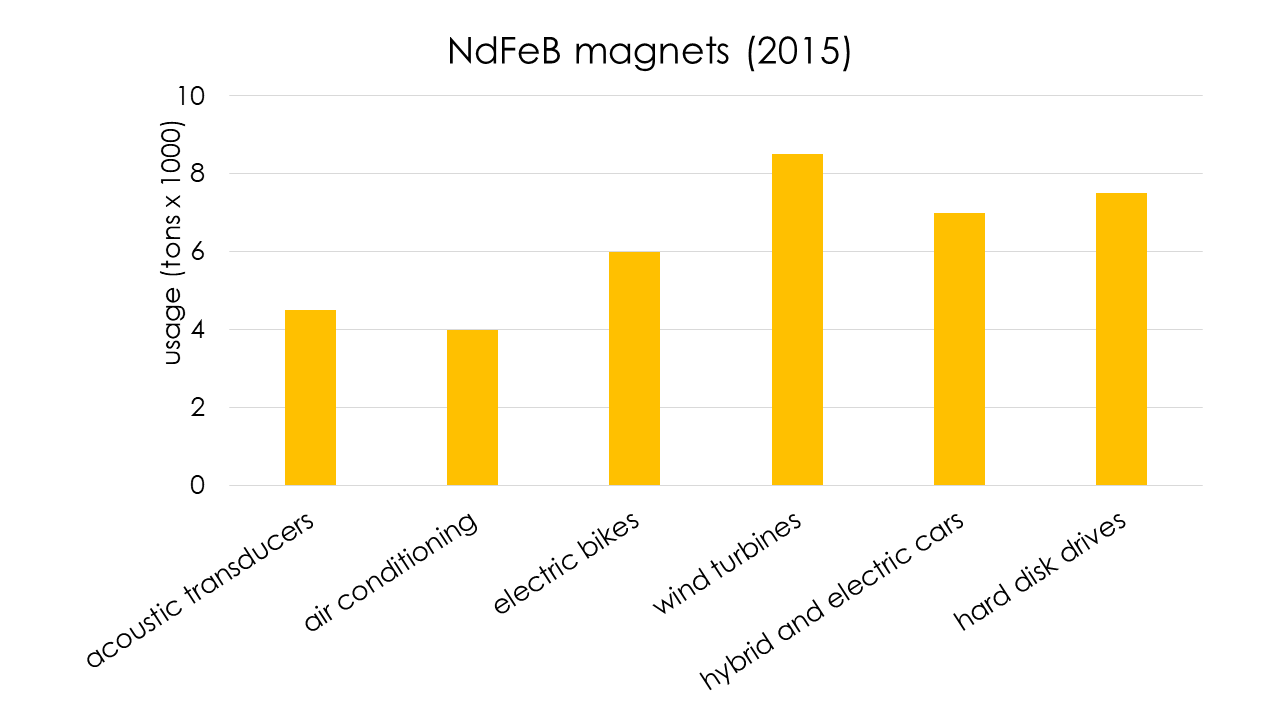
Figure 1: Usage of NdFeB magnets in the six major markets in the year 2015. Data taken from [3].

In many applications the NdFeB magnet are used at elevated temperature. For example, the operating temperature of the magnet in the motor/generator block of hybrid vehicles is at about 450 K. Though Nd₂Fe₁₄B ($T_{\mathrm{c}}=558$ K) shows excellent properties at room temperature its Curie temperature $T_{\mathrm{c}}$ is much lower than those of SmCo₅ ($T_{\mathrm{c}}=1020$ K) or Sm₂Co₁₇ ($T_{\mathrm{c}}=1190$ K) magnets [5]. Therefore the anisotropy field and the coercive field of Nd₂Fe₁₄B rapidly decays with increasing temperature. In order to compensate this loss, some of the magnet’s Nd is replaced with heavy rare earths such as Dy. Figure 2 compares the coercive field of conventional Dy-free and Dy-containing NdFeB magnets as a function of temperature. (NdDy)FeB magnets, containing around 10 weight percent Dy, can reach coercive fields $\mu_{0}H_{\rm c}>1$ T at 450 K. However, since the rare-earth crisis [6] the rare-earth prices have become more volatile. During 2010 and 2011 the Dy price peaked and increased by a factor of 20 [7]. Only four percent of the primary rare-earth production comes from outside China [6]. Because of supply risk and increasing demand, Nd and Dy are considered to be critical elements [8]. In order to cope with the supply risk, magnet producers and users aim for rare-earth free permanent magnets. With respect to the magnet’s performance, rare-earth free permanent magnets may fill a gap between ferrites and NdFeB magnets [9]. An alternative goal is magnets with less rare earth than (NdDy)FeB magnets but comparable magnetic properties [10].

Possible routes to achieve these goals are:

• Shape anisotropy based permanent magnets;

• Grain boundary diffusion;

• Improved grain boundary phases;

• Nanocomposite magnets;

• Alternative hard magnetic compounds.

In this work we will use micromagnetic simulations, in order to address various design issues for rare-earth efficient permanent magnets. Micromagnetic simulations are an important tool to understand coercivity mechanisms in permanent magnets. With the advance of hardware for parallel computing [11, 12, 13] and the improvement of numerical methods [14, 15, 16], micromagnetic simulations can take into account the microstructure of the magnet and thus help to understand how the interplay between intrinsic magnetic properties and microstructure impacts coercivity.

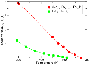
Figure 2: Coercive field of Nd₁₅Fe₇₇B₈ and (Nd_0.77Dy_0.33)₁₅Fe₇₇B₈ magnets as function of temperature. Data taken from [17].

1.2 Key properties of permanent magnets

The primary goal of a permanent magnet is to create a magnetic field in the air gap of a magnetic circuit. The energy stored in the field outside of a permanent magnet can be related to its magnetization and to its shape. According to Maxwell’s equations the magnetic induction $\mathbf{B}$ is divergence-free (solenoidal): $\nabla\cdot\mathbf{B}=0$ and in the absence of any current the magnetic field $\mathbf{H}$ is curl-free (irrotational): $\nabla\times\mathbf{H}=0$. The volume integral of the product of a solenoidal and irrotational vector field over all space is zero, when the corresponding vector and scalar potentials are regular at infinity [18]. This is the case when

$$\mathbf{B}=\mu_{0}(\mathbf{M}+\mathbf{H})$$ (1)

is the magnetic induction due to the magnetization $\mathbf{M}$ of a magnet. Here $\mu_{0}=4\pi\times 10^{-7}$ Tm/A is the permeability of vacuum. The magnetostatic energy in a volume $V_{\mathrm{a}}$ of free space, where $\mathbf{M}=0$ and $\mathbf{B}=\mu_{0}\mathbf{H}$, is $E_{\mathrm{mag,a}}=(\mu_{0}/2)\int_{V_{\mathrm{a}}}\mathbf{H}^{2}dV$. Splitting the space into the volume inside the magnet, $V_{\mathrm{i}}$, and $V_{\mathrm{a}}$, we have $\int\mathbf{B}\cdot\mathbf{H}dV=\int_{V_{\mathrm{a}}}\mu_{0}\mathbf{H}^{2}dV+\int_{V_{\mathrm{i}}}\mathbf{B}\cdot\mathbf{H}dV=0$ or

$$E_{\mathrm{mag,a}}=-\frac{1}{2}\int_{V_{\mathrm{i}}}\mathbf{B}\cdot\mathbf{H}dV.$$ (2)

Since the left-hand side of equation (2) is positive, $\mathbf{B}$ and $\mathbf{H}$ must point in opposite directions inside the magnet. Approximating the magnetic induction $\mathbf{B}$ and the magnetic field $\mathbf{H}$ by a uniform vector field inside the magnet, we can write $E_{\mathrm{mag,a}}=(1/2)\int_{V_{\mathrm{i}}}(BH)dV$, where $B=\left|\mathbf{B}\right|$ and $H=\left|\mathbf{H}\right|$. We see that we can increase the energy stored in its external field either by increasing the magnet’s volume $V_{\mathrm{i}}$ or by increasing the product $(BH)$, which is referred to as energy density product [19]. It is defined as the product of the magnetic induction $B$ and the corresponding opposing magnetic field $H$ [20] and is given in units of J/m³. When there are no field generating currents, the magnetic field inside the magnet

$$\mathbf{H}=-N\mathbf{M}$$ (3)

depends on the magnet’s shape which can be expressed by the demagnetizing factor $N$. We further assume that the magnet is saturated and there are no secondary phases so that $\left|\mathbf{M}\right|=M_{\mathrm{s}}$, where $M_{\mathrm{s}}$ is the spontaneous magnetization of the material. Using equations (1) and (3) we express the energy density product as $(BH)=\left|\mu_{0}(\mathbf{M}-N\mathbf{M})\right|\left|-N\mathbf{M}\right|=\mu_{0}(1-N)NM_{\mathrm{s}}^{2}$ [9, 21]. When maximized with respect to $N$ this gives the maximum energy density product of a given material

$$(BH)_{\mathrm{max}}=\frac{1}{4}\mu_{0}M_{\mathrm{s}}^{2}$$ (4)

for $N=1/2$. It is worth to check the shape of a magnet with a demagnetizing factor of $1/2$. Let us assume a magnet in form of a prism with dimensions $l\times l\times pl$ which is magnetized along the edge with length $pl$. Then a simple approximate equation for the demagnetizing factor is $N=1/(2p+1)$ [22]. Therefore, the optimum shape of a magnet that results in the maximum energy density product is a flat prism with dimensions $l\times l\times 0.5l$, which is twice as wide as high. Many modern magnets have this shape.

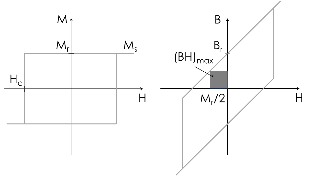
Figure 3: The maximum energy density product $(BH)_{\mathrm{max}}$ is given by the area of the largest rectangle that fits below the 2nd quadrant of the $B(H)$ curve. Left: $M(H)$ loop, right: $B(H)$ loop of an ideal magnet.

When there is no drop of the magnetization with increasing opposing field until $H>M_{\mathrm{s}}/2$, the energy density product reaches its maximum value given by equation (4). In this case, the magnetic induction $B$ as function of field is a straight line. For an ideal loop as shown in figure 3 the remanent magnetization, $M_{\mathrm{r}}$, equals the spontaneous magnetization, $M_{\mathrm{s}}$. In some materials, magnetization reversal may occur at fields lower than half the remanence. When $H_{\mathrm{c}}<M_{\mathrm{r}}/2$, the energy density product is limited by the coercive field, $H_{\mathrm{c}}$. Similarly, the maximum value for $(BH)_{\mathrm{max}}$ is not reached, when $M(H)$ is not square but decreases with increasing field $H$.

A higher energy density product reduces volume and weight of the permanent-magnet-containing device making it an important figure of merit. Other decisive properties are the remanence, the coercive field, and the loop squareness.

1.3 Permanent magnets and intrinsic magnetic properties

A magnetic material suitable for a permanent magnet must have certain intrinsic magnetic properties. From inspection of figure 3 we see that a good permanent magnet material requires a high spontaneous magnetization $M_{\mathrm{s}}$ and a uniaxial anisotropy constant $K$ that creates a coercive field

$$H_{\mathrm{c}}>\frac{M_{\mathrm{s}}}{2}.$$ (5)

The theoretical maximum for the coercive field is the nucleation field [23]

$$H_{\mathrm{N}}=\frac{2K}{\mu_{0}M_{\mathrm{s}}}$$ (6)

for magnetization reversal by uniform rotation of a small sphere. Equations (5) and (6) give the condition $K>\mu_{0}M_{\mathrm{s}}^{2}/4$. In other words, the anisotropy energy density, $K$, should be larger than the maximum energy density product, $(BH)_{\mathrm{max}}$. For most magnetic materials this condition is not sufficient [9]. There are two stronger conditions for the magnetocrystalline anisotropy constant.

To be able to make a permanent magnet or its constituents in any shape, the nucleation field must be higher than the maximum possible demagnetizing field. The demagnetizing factor of a thin magnet approaches 1 and the magnitude of the demagnetizing field approaches $M_{\mathrm{s}}$ which gives the condition $K>\mu_{0}M_{\mathrm{s}}^{2}/2$. This is often expressed in terms of the quality factor $Q={2K}/({\mu_{0}M_{\mathrm{s}}^{2}})$, which was introduced in the context of bubble domains in thin films [24, 25]. For $Q>1$ stable domains are formed and the magnetization points either up or down along the anisotropy axis perpendicular to the film plane. Otherwise, the demagnetizing field would cause the magnetization to lie in plane.

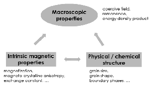
Figure 4: Both the intrinsic magnetic properties and the physical/chemical structure of the magnet determine coercive field, remanence and energy density product.

The maximum possible coercive field is never reached experimentally. This phenomenon is usually referred to as Brown’s paradox [26, 27]. Imperfections are one reason for the reduction of the coercive field with respect to its ideal value. In the presence of defects with zero magnetocrystalline anisotropy, the coercive field may reduce to $H_{\mathrm{c}}=H_{\mathrm{N}}/4$. Plugging this limit for the coercive field into equation (5) gives the condition $K>\mu_{0}M_{\mathrm{s}}^{2}$ for the anisotropy constant. This corresponds to the empirical law $\kappa>1$ for many hard magnetic phases of common permanent magnets [9], where $\kappa=\sqrt{{K}/({\mu_{0}M_{\mathrm{s}}^{2}})}$ is the hardness parameter [28].

The key figures of merit of permanent magnets such as the coercive field, the remanence, and the energy density product are extrinsic properties. They follow from the interplay of intrinsic magnetic properties and the granular structure of the magnet which is schematically shown in figure 4. Thus, in addition to the spontaneous magnetization $M_{\mathrm{s}}$, magnetocrystalline anisotropy constant $K$, and the exchange constant $A$, a well-defined physical and chemical structure of the magnet is essential for excellent permanent-magnet properties.

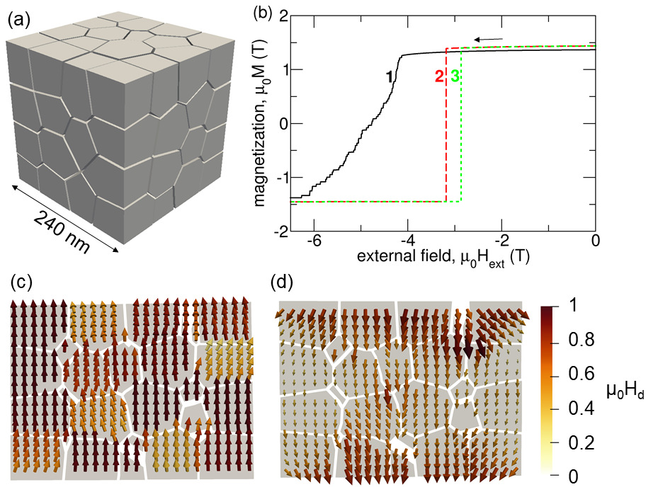
Figure 5: (a) Microstructure used for the simulation of microstructural effects that decrease the coercive field. (b) 1 misalignment (solid line) : non-magnetic grain boundary phase, demagnetizing field switched off; 2 Defects(dashed line): Weakly ferromagnetic grain boundary phase and demagnetization field switched off; 3 Demagnetizing effects: Weakly ferromagnetic grain boundary phase and demagnetization field switched on. The vector fields in (c) and (d) show magnetization and the demagnetizing field before switching for case 3.

Empirically, the effects that reduce the coercive field with respect to the ideal nucleation field are often written as [29, 30]

$$H_{\mathrm{c}}=\alpha_{K}\alpha_{\psi}H_{\mathrm{N}}-N_{\mathrm{eff}}M_{\mathrm{s}}-H_{\mathrm{f}}.$$ (7)

The coefficients $\alpha_{K}$ and $\alpha_{\psi}$ express the reduction in coercivity due to defects and misorientation, respectively [31]. The microstructural parameter $N_{\mathrm{eff}}$ is related to the effect of the local demagnetization field near sharp edges and corners of the microstructure [32]. The fluctuation field $H_{\mathrm{f}}$ gives the reduction of the coercive field by thermal fluctuations [33].

Let us look at an example. Figure 5a shows the microstructure of a nanocrystalline Nd₂Fe₁₄B magnet used for micromagnetic simulations to identify the different effects that reduce coercivity. For the set of material parameters used ($K=4.3$ MJ/m³, $\mu_{0}M_{\mathrm{s}}=1.61$ T, $A=7.7$ pJ/m), the ideal nucleation field is $\mu_{0}H_{\mathrm{N}}=6.7$ T. The 64 grains were generated from a centroid Voronoi tessellation [34]. The average grain size was 60 nm. The anisotropy directions were randomly distributed within a cone with an opening angle of 15 degrees. The grain boundary phase of NdFeB magnets contains Fe and is weakly ferromagnetic [35, 36, 37]. In addition to magnetostatic interactions between the grains, the grains are also weakly exchange coupled. In our simulations the grain boundary phase was 3 nm thick. The magnetocrystalline anisotropy constant $K$ of the grain boundary phase was zero. Its magnetization and exchange constant were $\mu_{0}M_{\mathrm{s}}=0.5$ T and $A=7.7$ pJ/m for cases 2 to 4.

In numerical micromagnetics we can artificially switch physical effects on or off and thus gain a deeper understanding of how the various effects impact magnetization reversal. We start with the granular system whereby the grains are separated by a nonmagnetic grain boundary phase and the magnetostatic energy term is switched off. Thus, there are no demagnetizing fields and no magnetostatic interactions. The grains are isolated and there are no defects. The solid line (case 1) of figure 5b shows the influence of misalignment on magnetization reversal. Owing to the different easy directions the grains switch at slightly different values of the external field. The coercive field is $\mu_{0}H_{\mathrm{c}}=4.77$ T. With $\alpha_{K}=1$, $N_{\mathrm{eff}}=0$, and $H_{\mathrm{f}}=0$ which hold for case 1 per definition, we obtain $\alpha_{\psi}=0.71$ from equation (7). For the computation of the dashed line (case 2) we assume a weakly ferromagnetic grain boundary phase. The magnetostatic terms are not taken into account. The grain boundary phase acts as a soft magnetic defect and reduces coercivity. The corresponding microstructural parameter is $\alpha_{K}=0.67$. Owing to exchange coupling between the grains all grains reverse at the same external field. For the dotted line (case 3) we switch on the demagnetizing field. The magnetization and the demagnetizing field are shown in a slice through the grains in figures 5c and 5d, respectively. The reduction of the coercive field owing to demagnetizing effects equates to $N_{\mathrm{eff}}=0.2$. Finally, we take into account thermal activation by computing the energy barrier for the nucleation of reversed domains as function of field [38]. The decrease of coercivity by thermal activation is $\mu_{0}H_{\mathrm{f}}=0.23$ T.

2 Micromagnetics of permanent magnets

2.1 Micromagnetic energy contributions

Micromagnetism is a continuum theory that handles magnetization processes on a length scale that is small enough to resolve the transition of the magnetization within domain walls but large enough to replace the atomic magnetic moments by a continuous function of position [39]. The state of the magnet is described by the magnetization $\mathbf{M}$, whose magnitude $\left|\mathbf{M}\right|=M_{\mathrm{s}}$ is constant and whose direction $\mathbf{m}=\mathbf{M}/M_{\mathrm{s}}$ is continuous. A stable or metastable magnetic state can be found by finding a function $\mathbf{m}=\mathbf{m}(\mathbf{r})$ with $\left|\mathbf{m}\right|=1$ that minimizes the Gibbs free energy of the magnet

$$E(\mathbf{m})= \int_{V}\left[A\left(\left(\nabla m_{x}\right)^{2}+\left(\nabla m_{y}\right)^{2}+\left(\nabla m_{z}\right)^{2}\right)\right.$$ (11)

$$\qquad-K\left(\mathbf{m}\cdot\mathbf{k}\right)^{2}$$

$$\qquad-\frac{\mu_{0}M_{\mathrm{s}}}{2}\left(\mathbf{m}\cdot\mathbf{H}_{\mathrm{d}}\right)$$

$$\Big{.}\qquad-\mu_{0}M_{\mathrm{s}}\left(\mathbf{m}\cdot\mathbf{H}_{\mathrm{ext}}\right)\Big{]}dV.$$

The different lines describe the exchange energy, the magnetocrystalline anisotropy energy, the magnetostatic energy, and the Zeeman energy, respectively. The coefficients $A$, $K$, and $M_{\mathrm{s}}$ in equation (11) to (11) vary with position and thus represent the microstructure of the magnet. The unit vector along the anisotropy direction, $\mathbf{k}$, varies from grain to grain reflecting the orientation of the grains. The anisotropy constant $K$ will be zero in local defects or within the grain boundary phase. The grain boundary phase may be weakly ferromagnetic with magnetization $M_{\mathrm{s}}$ and the exchange constant $A$ considerably reduced with respect to the bulk values. In $\alpha$-Fe inclusions $K$ is negligible and $M_{\mathrm{s}}$ and $A$ are high. Composite magnets combine grains with different intrinsic properties. The demagnetizing field $\mathbf{H}_{\mathrm{d}}$ arises from the divergence of the magnetization. The factor 1/2 in equation (11) indicates that it is a self-energy which depends on the current state of $\mathbf{M}$. It can be calculated from the static Maxwell’s equations. One common method is the numerical solution of the magnetostatic boundary value problem for the magnetic scalar potential $U$ where the demagnetizing field is derived as $\mathbf{H}_{\mathrm{d}}=-\nabla U$. The magnetic scalar potential fulfills the Poisson equation

$$\nabla^{2}U=\mathbf{\nabla}\cdot\mathbf{M}$$ (12)

inside the magnet, the Laplace equation

$$\nabla^{2}U=0$$ (13)

outside the magnet, and the interface conditions

$$U^{\mathrm{(in)}}=U^{\mathrm{(out)}}$$ (14)

$$\left(U^{\mathrm{(in)}}-U^{\mathrm{(out)}}\right)\cdot\mathbf{n}=\mathbf{M}\cdot\mathbf{n}$$ (15)

at the magnet’s boundary with unit surface normal $\mathbf{n}$. Equation (14) follows from the continuity of the component of the magnetic field $\mathbf{H}$ parallel to the surface (which follows from $\mathbf{\nabla}\times\mathbf{H}=0$). Equation (15) follows from the continuity of the component of the magnetic induction $\mathbf{B}$ normal to the surface (which follows from $\nabla\cdot\mathbf{B}=0$) [40].

2.2 Numerical methods

2.2.1 Hysteresis

There is no unique constrained minimum for equation (11) to (11) for a given external field. The magnetic state that a magnet can access depends on its history. Hysteresis in a non-linear system results from the path formed by subsequent local minima [41]. In permanent magnet studies we are interested in the demagnetization curve. Thus, we use the saturated state as initial state and compute subsequent energy minima for a decreasing applied field, $H_{\mathrm{ext}}$. The projection of the magnetization onto the direction of the applied field integrated over the volume of the magnet, that is $\int_{V}M_{\mathrm{s}}\left(\mathbf{m}\cdot\mathbf{H}_{\mathrm{ext}}/\left|\mathbf{H}_{\mathrm{ext}}\right|\right)dV$, as function of different values of $H_{\mathrm{ext}}$ gives the $M(H_{\mathrm{ext}})$-curve. For computing the maximum energy density product we need the $M(H)$-curve, where $H$ is the internal field $H=H_{\mathrm{ext}}-NM(H_{\mathrm{ext}})$. Similar to open circuit measurements [42] we correct $M(H_{\mathrm{ext}})$ with the macroscopic demagnetizing factor $N$ of the sample, in order to obtain $M(H)$.

2.2.2 Finite element and finite difference discretization

The computation of the energy for a permanent magnet requires the discretization of equations (11) to (11) taking into account the local variation of $M_{\mathrm{s}}$, $K$, and $A$, according to the microstructure. Common discretization schemes used in micromagnetics for permanent magnets [43] are the finite difference method [13] or the finite element method [15, 14].

Each node of a finite element mesh or cell of a finite difference scheme with index $i$ holds a unit magnetization vector $\mathbf{m}_{i}$. We gather these vectors into the vector $\mathbf{x}$ which has the dimension $3n$, where $n$ is the number of nodes or cells. Then the Gibbs free energy may be written as [14]

$$E(\mathbf{x})=\frac{1}{2}\mathbf{x}^{\mathrm{T}}\mathbf{C}\mathbf{x}-\frac{\mu_{0}}{2}\mathbf{h}_{\mathrm{d}}^{\mathrm{T}}\bar{\mathbf{M}}\mathbf{x}-\mu_{0}\mathbf{h}_{\mathrm{ext}}^{\mathrm{T}}\bar{\mathbf{M}}\mathbf{x}.$$ (16)

The three terms on the right-hand side of (16) from left to right are the sum of the exchange and anisotropy energy, the magnetostatic self-energy, and the Zeeman energy, respectively. The sparse matrix $\mathbf{C}$ contains grid information associated with the discretization of the exchange and anisotropy energy. The matrix $\bar{\mathbf{M}}$ accounts for the local variation of the saturation magnetization $M_{\mathrm{s}}$ within the magnet. It is a diagonal matrix whose entries are the modulus of the magnetic moment associated with the node or cell $i$ [14]. The vectors $\mathbf{x}$, $\mathbf{h}_{\mathrm{d}}(\mathbf{x})$, and $\mathbf{h}_{\mathrm{ext}}$ hold the unit vectors of the magnetization, the demagnetizing field, and the external field at the nodes of the finite element mesh or the cells of a finite difference grid, respectively.

For computing the demagnetizating field, equations (12) to (15) can be solved using an algebraic multigrid method on the finite element mesh [44, 45, 14].

In finite difference methods the magnetization is assumed to be uniform within each cell. Then the magnetic field generated at point $\mathbf{r}$ by the magnetization in cell $j$ is given by an integration over the magnetic surface charges $\sigma_{j}=M_{\mathrm{s}j}\mathbf{m}_{j}\cdot\mathbf{n}$ [46],

$$\mathbf{H}_{\mathrm{d},j}(\mathbf{r})=-\frac{1}{4\pi}\nabla\left(\int_{\partial V_{j}}\frac{\sigma_{j}^{\prime}}{\left|\mathbf{r}-\mathbf{r}^{\prime}\right|}dS_{j}^{\prime}\right),$$ (17)

where $\mathbf{n}$ is the unit surface normal. The magnetostatic energy is a double sum over all computational cells

$$E_{\mathrm{m}}=-\frac{\mu_{0}}{2}\sum_{i}M_{\mathrm{s,i}}\mathbf{m}_{i}\cdot\int_{V_{i}}\sum_{j}\mathbf{H}_{\mathrm{d},j}(\mathbf{r})dV.$$ (18)

Applying integration by parts we can rewrite the magnetosatic energy as [47]

$$E_{\mathrm{m}}=\frac{\mu_{0}}{8\pi}\sum_{i,j}\int_{\partial V_{i}}\int_{\partial V_{j}}\frac{\sigma_{i}\sigma_{j}^{\prime}}{\left|\mathbf{r}-\mathbf{r}^{\prime}\right|}dS_{j}^{\prime}dS_{i}.$$ (19)

Introducing the demagnetization tensor $\mathbf{N}_{ij}$ reduces equation (19) to

$$E_{\mathrm{m}}=\frac{\mu_{0}}{2}V_{\mathrm{cell}}\sum_{i,j}M_{\mathrm{s}i}\mathbf{m}_{i}\mathbf{N}_{ij}M_{\mathrm{s}j}\mathbf{m}_{j},$$ (20)

where $V_{\mathrm{cell}}$ is the volume of a computational cell. The term $\mu_{0}V_{\mathrm{cell}}M_{\mathrm{s}i}\mathbf{m}_{i}\mathbf{N}_{ij}M_{\mathrm{s}j}\mathbf{m}_{j}$ is the magnetostatic interaction energy between cells $i$ and $j$. From equation (20) we can compute the cell averaged demagnetizing field [48, 49]

$$\mathbf{h}_{i}=-\sum_{j}\mathbf{N}_{ij}M_{\mathrm{s}j}\mathbf{m}_{j}.$$ (21)

The demagnetization tensor $\mathbf{N}_{ij}$ depends only on the relative distance between the cells $i$ and $j$. The convolution (21) can be efficiently computed using Fast Fourier Transforms. Special implementations of the Fast Fourier Transform with low communication overhead makes large-scale simulations of permanent magnets possible on supercomputers with thousands of cores [13].

2.2.3 Energy minimization

The intrinsic time scale of magnetization processes is related to the Lamor frequency $f=\gamma\mu_{0}H/(2\pi)$. The gyromagnetic ratio is $\gamma=1.76086\times 10^{11}$/(Ts). For example, let us estimate the intrinsic time scale for precession in Nd₂Fe₁₄B. The magnitude of typical internal fields, $\mu_{0}H$ are about a few Tesla. The Lamor frequency is 28 GHz per Tesla. This gives a characteristic time scale smaller than $10^{-10}$ s. Such time scales may be relevant for magnetic recording or spin electronic devices. In permanent magnet applications the rate of change of the external field is much slower. For example, low speed direct drive wind mills run at about 20 rpm [50] and motors of hybrid vehicles run at 1500 rpm to 6000 rpm [51], which translate into frequencies ranging from 1/3 Hz to 100 Hz. The magnetization always reaches metastable equilibrium before a significant change of the external field. Based on this argument many researchers use energy minimization methods for simulation of magnetization reversal in permanent magnets, taking advantage of a significant speedup as compared to time integration solvers [15, 11].

Minimizing equation (16) subject to the unit norm constraint for decreasing external field gives the magnetic states along the demagnetization curve of the magnet. The sparse matrix $\mathbf{C}$ and the diagonal matrix $\bar{\mathbf{M}}$ depend only on the geometry and the intrinsic magnetic properties. The vector $\mathbf{h}_{\mathrm{d}}$ depends linearly on the magnetization. Evaluation of the energy, its gradient, or the Hessian requires the solution of the magnetostatic subproblem. The magnetic field depends linearly on the magnetization. Thus, (16) is quadratic in $\mathbf{x}$. However, the condition $\mathbf{M}=M_{\mathrm{s}}$ implies that each subvector $\mathbf{m}_{i}$ of $\mathbf{x}$ is constrained to be a unit vector. The optimization problem is supplemented by $n$ nonlinear constraints $\left|\mathbf{m}_{i}\right|=1,\;i=1,...,n$.

In its most simple form an algorithm for energy minimization (see algorithm 1) is an iterative process with the following four tasks per iteration: The computation of the search direction, the computation of the step length, the motion towards the minimum, and the check for convergence. These computations make use of the objective function $E(\mathbf{x})$ and its gradients, possibly second derivatives and maybe information gathered from previous iterations. The superscript ⁺ marks quantities which are computed for the next iteration step. The superscript ^- marks quantities which have been computed during the previous iteration step.

Algorithm 1 minimize $E(\mathbf{x})$

repeat

     compute search direction $\mathbf{d}$

     compute step length $\alpha$

     proceed $\mathbf{x}^{+}=\mathbf{x}+\alpha\mathbf{d}$

until $convergence$

Variants of the steepest-descent method, [11, 52, 53, 54], the non-linear conjugate gradient method [14, 15], and the quasi-Newton method [55, 56, 57] are most widely used in micromagnetics for permanent magnets. In steepest-descent methods the search direction is the negative gradient $\mathbf{g}=\nabla E(\mathbf{x})$ of the energy: $\mathbf{d}=-\mathbf{g}$. The nonlinear conjugate-gradient method uses a sequence of conjugate directions $\mathbf{d}=-\mathbf{g}+\beta\mathbf{d}^{-}$. The Newton method uses the negative gradient multiplied by the inverse of the Hessian matrix: $\mathbf{d}=-(\nabla^{2}E)^{-1}\nabla\mathbf{g}$ as search direction. In quasi-Newton methods the inverse of the Hessian is approximated by information gathered from previous iterations.

The step length $\alpha$ is obtained by approximate line search minimization. To that end the new point is determined along the line defined by the current search direction and should yield a sufficiently smaller energy with a sufficiently small gradient (approximate local minimum along the line). By expanding and shrinking a search interval for $\alpha$, line search algorithms [58] find an appropriate step length. Owing to the solution of the magnetostatic subproblem, evaluations of the energy are expensive. In order to reduce the number of energy evaluations Koehler and Fredkin [59] apply an inexact line search based on cubic interpolation. Tanaka and co-workers [15] propose to interpolate the magnetostatic field within the search interval if it is sufficiently small. Fischbacher et al. [14] showed that long steps should be avoided, in order to compute all metastable states along the demagnetization curve. They suggest applying a single Newton step in one dimension to get an initial estimate for the step length which then may be further reduced to fulfill the sufficient decrease condition. For steepest descent methods Barzilai and Borwein [60] proposed a step length $\alpha$ such that $\alpha$ multiplied with the identity matrix, $\mathbf{1}$, approximates the inverse of the Hessian matrix: $\alpha\mathbf{1}\approx(\nabla^{2}E)^{-1}$. Thus, the Barzilai-Borwein method makes use of the key idea of limited memory quasi Newton methods applied to step length selection. The step length is computed from information gathered during the last 2 iteration steps. This method was successfully applied in numerical micromagnetics [11, 61, 62].

When applied to micromagnetics the update rule $\mathbf{x}^{+}=\mathbf{x}+\alpha\mathbf{d}$ will not preserve the norm of the magnetization vector. A simple cure is renormalization $\mathbf{m}^{+}_{i}=(\mathbf{m}_{i}+\alpha\mathbf{d}_{i})/\left|(\mathbf{m}_{i}+\alpha\mathbf{d}_{i})\right|$. When certain conditions for $\mathbf{d}$ [63] and the computational grid [64] are met the normalization leads to a decrease in the energy. One condition [63] for an energy decrease upon normalization is that the search direction is perpendicular to the magnetic state of the current point: $\mathbf{m}_{i}\cdot\mathbf{d}_{i}$ for all $i$. Following Cohen et al. [65] we can replace the energy gradient by its projection onto its component perpendicular to the local magnetization

$$\hat{\mathbf{g}}_{i}=\mathbf{g}_{i}-\left(\mathbf{g}_{i}\cdot\mathbf{m}_{i}\right)\mathbf{m}_{i}=-\mathbf{m}_{i}\times\left(\mathbf{m}_{i}\times\mathbf{g}_{i}\right).$$ (22)

In nonlinear conjugate gradient methods the search directions are linear combinations of vectors perpendicular to the magnetization (the current projected gradient and the previous search directions initially being the projected gradient). Instead of updating and normalization, the vectors $\mathbf{m}_{i}$ might also be rotated by an angle $\alpha\left|\mathbf{d}_{i}\right|$ [66] or a norm conserving semi-implicit update rule [67] may be applied.

The right-hand side of equation (22) follows from the vector identity $\mathbf{a}\times\left(\mathbf{b}\times\mathbf{c}\right)=\left(\mathbf{a}\cdot\mathbf{c}\right)\mathbf{b}-\left(\mathbf{a}\cdot\mathbf{b}\right)\mathbf{c}$ and $\left|\mathbf{m}_{i}\right|=1$. On computational grids with a uniform mesh the energy gradient is proportional to the effective field

$$\mathbf{h}_{\mathrm{eff}i}=-\frac{1}{\mu_{0}M_{\mathrm{s}i}V_{\mathrm{cell}}}\mathbf{g}_{i}.$$ (23)

By inspecting the right-hand side of equation (22), we see that the search direction of a steepest-descent method is proportional to the damping term of the Landau-Lifshitz equation [68]. Time integration of the Landau-Lifshitz-Gilbert equation without the precession term [52] is equivalent to minimization by the steepest-descent method. Furaya et al. [52] use a semi-implicit time integration scheme. They split the effective field into its local part and the long-ranging magnetostatic field which not only depends on the nearest neighbor cells but on the magnetization in the entire magnet. By treating the local part of the effective field implicitly and the magnetostatic field explicitly, much larger time steps and thus faster convergence toward the energy minimum is possible.

There are several possible termination criteria for a minimization algorithm. Koehler and Fredkin [59] used the relative change in the energy between subsequent iterations. Others [52, 13] use the difference between the subsequent magnetic states. Gill et al. [69] recommend a threefold criterion taking into account the change in energy, the change in the magnetic state, and the norm of the gradient for unconstrained optimization. This ensures convergence of the sequence of the magnetic states, avoids early stops in flat regions and ensures progress towards the minimum.

2.2.4 Time integration

The torque on the magnetic moment $\mathbf{M}V_{\mathrm{cell}}$ of a computational cell in a magnetic field $\mathbf{H}$ is $\mathbf{T}=\mu_{0}\mathbf{M}V_{\mathrm{cell}}\times\mathbf{H}$. The angular momentum associated with the magnetic moment is $\mathbf{L}=-\mathbf{M}V_{\mathrm{cell}}/\left|\gamma\right|$. The change of the angular momentum with time equals the torque, $\partial\mathbf{L}/\partial t=\mathbf{T}$. Applying the torque equation for the magnetic volume which is divided into computational cells gives

$$\frac{\partial\mathbf{m}_{i}}{\partial t}=-\left|\gamma\right|\mu_{0}\mathbf{m}_{i}\times\mathbf{h}_{\mathrm{eff}i},$$ (24)

which describes the precession of the magnetic moment around the effective field. In order to describe the motion of the magnetization towards equilibrium, equation (24) has to be augmented with a damping term. Following Landau and Lifshitz [68] we can add a term $-\lambda\mathbf{m}_{i}\times\left(\mathbf{m}_{i}\times\mathbf{h}_{\mathrm{eff}i}\right)$ to the right-hand side of equation (24) which will move the magnetization towards the field. Alternatively we can - as suggested by Gilbert [70] - add a dissipative force $-\alpha\partial\mathbf{m}_{i}/\partial t$ to the effective field. The precise path the system follows towards equilibrium depends on the type of equation used and the value of the damping parameters $\lambda$ or $\alpha$. In the Landau-Lifshitz equation precession is not changed with increasing damping, whereas in the Gilbert case an increase of the damping constant slows down precessional motion. Only for small damping the Landau Lifshitz equation and the Gilbert equation are equivalent. This can be seen if the Gilbert equation is written in Landau-Lifshitz form [71]

$$\frac{\partial\mathbf{m}_{i}}{\partial t} = -\frac{\left|\gamma\right|\mu_{0}}{1+\alpha^{2}}\mathbf{m}_{i}\times\mathbf{h}_{\mathrm{eff}i}$$ (25)

$$-\alpha\frac{\left|\gamma\right|\mu_{0}}{1+\alpha^{2}}\mathbf{m}_{i}\times\left(\mathbf{m}_{i}\times\mathbf{h}_{\mathrm{eff}i}\right).$$

In the limit of high damping only the second term of equation (25) remains and the time integration of the Landau-Lifshitz-Gilbert equation becomes equivalent to the steepest-descent method. For coherent rotation of the magnetization the minimum reversal time occurs for a damping parameter $\alpha=1$. In turn, fast reversal reduces the total computation time. This is the motivation for using a damping parameter $\alpha=1$ for simulation of magnetization reversal in permanent magnets [72, 66] by numerical integration of equation (25). Several public domain micromagnetic software tools use solvers for the numerical solution of equation(25) based on the adaptive Euler methods [73], Runge-Kutta schemes [62], backward-differentiation methods [74], and preconditioned implicit solvers [75].

2.2.5 Energy barriers

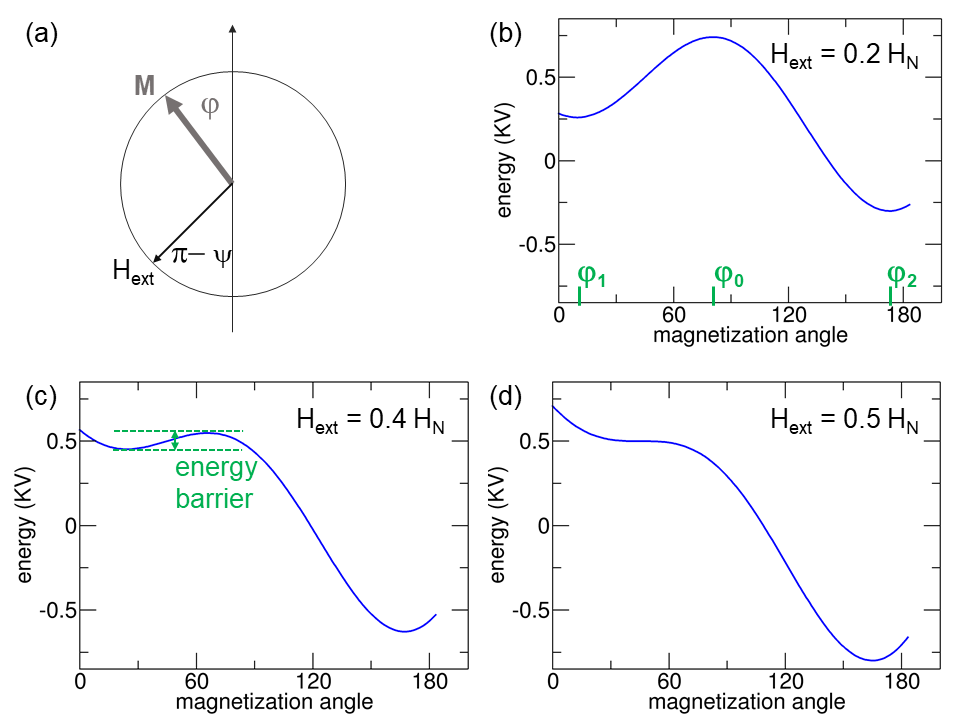
Figure 6: Energy landscape as function of the magnetization angle. (a) Small hard magnetic sphere in an external field. The field is applied at an angle of $\pi-\psi=45$ degrees. (b) to (d) With increasing field the energy barrier decreases.

Permanent magnets are used at elevated temperature. However, classical micromagnetic simulations take into account temperature only by the temperature-dependent intrinsic materials properties. Thermal fluctuations that may drive the system over a finite energy barrier are neglected. Before magnetization reversal, a magnet is in a metastable state. With increasing opposing field the energy barrier decreases. The system follows the local minima reversibly until the energy barrier vanishes and the magnetization changes irreversibly [76]. If the height of the energy barrier is around $25k_{\mathrm{B}}T$, thermal fluctuations can drive the system over the barrier within a time of approximately one second [77]. To illustrate this behavior, let us look at the energy landscape of a small hard magnetic sphere with volume $V$ (see figure 6). The energy per unit volume is $E(\varphi,H_{\mathrm{ext}})/V=K\sin^{2}(\varphi)-\mu_{0}M_{\mathrm{s}}H_{\mathrm{ext}}\cos(\varphi-\psi)$. The external field is applied at an angle $\psi$ with respect to the positive anisotropy axes. For small external fields the energy shows two minima as function of the magnetization angle $\varphi$. The state before switching is given by $\varphi_{1}=(\pi-\psi)M_{\mathrm{s}}H_{\mathrm{ext}}/(2K-M_{\mathrm{s}}H_{\mathrm{ext}})$ and the state after switching is given by $\varphi_{2}=\pi-(\pi-\psi)M_{\mathrm{s}}H_{\mathrm{ext}}/(2K+M_{\mathrm{s}}H_{\mathrm{ext}})$. The maximum energy occurs at the saddle point at $\varphi_{0}=\sqrt[3]{-\tan\psi}$ [78].

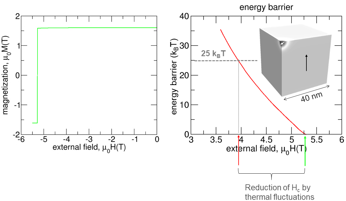
Figure 7: Thermally induced magnetization reversal in a Nd₂Fe₁₄B cube. Left: Computed demagnetization curve by classical micromagnetics. Right: Energy barrier for the formation of a reversed nucleus as a function of the applied field. The inset shows the saddle point configuration of the magnetization. Data taken from [30].

In permanent magnets magnetization reversal occurs by the nucleation and expansion of reversed domains [79]. Similar to the situation depicted in figure 6 the nucleation of a reversed domain or the depinning of a domain wall is associated with an energy barrier that is decreased by an increasing external field. Using the elastic band method [80] or the string method [81] the energy barrier can be computed as function of the external field. The critical field at which the energy barrier $E_{\mathbf{B}}(H_{\mathrm{ext}})$ crosses the $25k_{\mathrm{B}}T$-line is the coercive field of the magnet taking into account thermal fluctuations. The elastic band method and the string method are well-established path finding methods in chemical physics [82, 83]. In micromagnetics they can be used to compute the minimum energy path that connects the local minimum at field $H_{\mathrm{ext}}$ with the reversed magnetic state. A path is called a minimum energy path if for any point along the path the gradient of the energy is parallel to the path. In other words, the component of the energy gradient normal to the path is zero. The string method can be easily applied by subsequent application of a standard micromagnetic solver. It is an iterative algorithm: The magnetic states along the path are described by images. Each image is a replica of the total system. A single iteration step consists of two moves. (1) Each image is relaxed by applying a few steps of an energy minimization method or by integrating the Landau-Lifshitz-Gilbert equation for a very short time. (2) The images are moved along the path such that the distance between the images is constant. Within the framework of the elastic band method images may only move perpendicular to the current path and the distance between the images is kept constant with a virtual spring force. For an accurate computation of the energy barrier for a nucleation process [83] variants of the string method exists which keep more images next to the saddle point. This can be achieved by an energy weighted distance function between the images [84] and truncation of the path [85].

Figure 7 compares the coercive field of a Nd₂Fe₁₄B cube with an edge length of 40 nm obtained by classical micromagnetic simulations and computing energy barriers as discussed above. In both methods the intrinsic magnetic material parameters for $T=300$ K were used. The non-zero temperature coercive field, which takes into account thermal fluctuations, is defined as the critical value of the external field at which the energy barrier reaches $25k_{\mathrm{B}}T$. By inspecting the magnetic states along the minimum energy path we can see how thermally induced magnetization reversal happens. At the saddle point a small reversed nucleus is formed. If there is no barrier for the expansion of the reversed domain, the reversed domain grows and the particle will switch. The simulations are self-consistent: The coercive field calculated by classical micromagnetics equals the field at which the energy barrier vanishes. For nearly ideal particles such as the cube without soft magnetic defects discussed above, the reduction of the coercive field by thermal fluctuations may be as large as 25 percent [86]. However, the presence of defects reduces the decay of coercivity owing to thermal fluctuations [30]. For example for the magnetic structure in figure 2, which contains a weakly ferromagnetic grain boundary, thermal fluctuations reduce the coercive field by only 8 percent.

Energy barriers for reversal may also be computed by atomstic spin dynamics. Miyashita et al. [87, 88] solved equation (25) numerically for atomic magnetic moments augmented by a stochastic thermal field. From the computed relaxation time, $\tau$, at a fixed external field the energy barrier can be computed by fitting the results to an Arrhenius-Neel law $\tau=(1/f_{0})\exp(E_{\mathrm{B}}/(k_{\mathrm{B}}T))$ or to Sharrock’s law [89], which gives the coercive field as function of $H_{\mathrm{ext}}$ and $\tau$. Alternatively, Toga et al. used the constrained Monte-Carlo method [90] to compute field dependent energy barriers for an atomistic spin model.

In equation (7) we attributed the reduction of coercivity to the fluctuation field $H_{\mathrm{f}}$. The energy barrier for magnetization reversal is related to this fluctuation field by $H_{\mathrm{f}}=-25k_{\mathrm{B}}T/(\partial E/\partial H_{\mathrm{ext}})$. Experimentally, the energy barrier or the fluctuation field can be obtained by measuring the magnetic viscosity which is related to the change of magnetization with time at a fixed external field. It was measured by Givord et al. [91], Villas-Boas [92], and Okamota et al. [93] for sintered, melt-spun, and hot-deformed magnets, respectively.

2.3 Microstructure representation

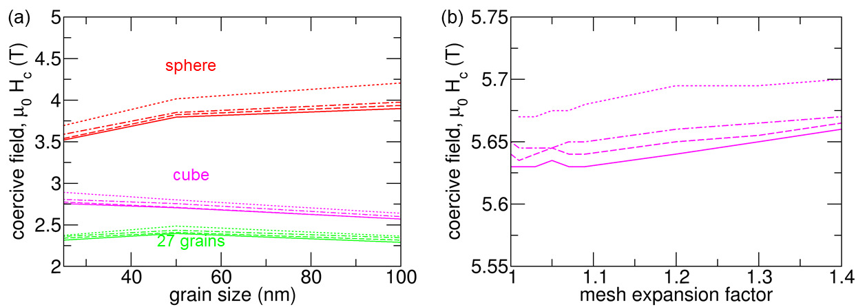
Figure 8: (a) Coercive field of a sphere, a cube, and a polycrystalline magnet as function of grain size. The grains are made of Nd₂F₁₄B and surrounded by a 3 nm thick, weakly-ferromagnetic grain boundary phase. The grain size is defined as $\sqrt[3]{V_{\mathrm{grain}}}$, where $V_{\mathrm{grain}}$ is the volume of the grain. (b) Coercive field of the 100 nm pure Nd₂F₁₄B cube as function of the expansion factor $a$ in a geometrical mesh. The solid, dashed, dot-dashed, and dotted line refer to a mesh size of 1.3 nm, 2 nm, 2.7 nm, and 4 nm, respectively, defined at the surface of the cube.

2.3.1 Grain size and particle shape

The discretization of the Gibb’s free energy by finite differences or finite elements poses a question concerning the required grid size. The required grid size is related to the characteristic length scale of inhomogeneities in the magnetization, which is related to the relative weight of the exchange energy to other contributions of the Gibb’s free energy.

Upon minimization the exchange energy favors a uniform magnetization with the local magnetic moments on the computational grid parallel to each other. The accurate computation of the critical field for the formation of a reversed nucleus requires the energy of the domain wall, which separates the nucleus from the rest, to be known with high accuracy. Therefore, we should be able to resolve the transition of the magnetization within the domain wall on the computational grid. The width of a Bloch wall is $\delta_{\mathrm{B}}=\pi\delta_{0}$. The Bloch wall parameter $\delta_{0}=\sqrt{A/K}$ denotes the relative importance of the exchange energy versus crystalline anisotropy energy.

Whereas in ellipsoidal particles the demagnetizing field is uniform, it is inhomogeneous in polyhedral particles. The non-uniformity of the demagnetizing field strongly influence magnetization reversal [94]. Near edges or corners [32] the transverse component of the demagnetizing field diverges. Owing to the locally increased demagnetizing field, the reversed nucleus will form near edges or corners [95] (see also figure 7). We have to correctly resolve the rotations of the magnetization that eventually form the reversed nucleus. For the computation of the nucleation field the required minimum mesh size has to be smaller than the exchange length $l_{\mathrm{ex}}=\sqrt{A/(\mu_{0}M_{\mathrm{s}}^{2}/2)}$ at the place where the initial nucleus is formed. It gives the relative importance of the exchange energy versus magnetostatic energy. Please note that sometimes the exchange length is also defined as $l_{\mathrm{lex}}=\sqrt{A/(\mu_{0}M_{\mathrm{s}}^{2})}$ [96, 5]. In order to keep the computation time low and resolve important magnetization processes, Schmidts and Kronmüller introduced a graded mesh that is refined towards the edges [97].

The relative importance of the different energy terms also explains the grain size dependence of coercivity. The coercive field of permanent magnets decreases with increasing grain size [97, 98, 99, 100, 101]. The smaller the magnet the more dominant is the exchange term. Thus, it costs more energy to form a domain wall. To achieve magnetization reversal, the Zeeman energy of the reversed magnetization in the nucleus needs to be higher. This can be accomplished by a larger external field.

In the following numerical experiment we computed the coercive field of a sphere, a cube, and a magnet consisting of 27 polyhedral grains. The polycrystalline magnet is shown in figure 9. We computed the coercive field as function of the size of the magnet for different finite element meshes. We used the conjugate gradient method [14] to compute the magnetic states along the demagnetization curve. The Nd₂Fe₁₄B particles ($K=4.9$ MJ/m³, $\mu_{0}M_{\mathrm{s}}=1.61$ T, $A=8$ pJ/m [5]) were covered by a soft magnetic phase with a thickness of 3 nm. In the polycrystalline sample the grains are also covered by a 3 nm soft phase which adds up to a 6 nm thick grain boundary. The material parameters of the grain boundary phase $K=0$, $\mu_{0}M_{\mathrm{s}}=0.477$ T, and $A=6.12$ pJ/m correspond to a composition of Nd₄₀Fe₆₀ [102]. The characteristic lengths for the main phase are $\delta_{0}=1.3$ nm, $\delta_{\mathrm{B}}=4$ nm, and $l_{\mathrm{ex}}=2.8$ nm. The exchange length for the boundary phase is $l_{\mathrm{ex}}=8.2$ nm. The results are summarized in figure 8a which gives the coercive field as function of grain size. The three sets of curves are for the sphere, the cube, and the polycrystalline magnet. The different curves within a set correspond to a mesh size of 1.3 nm, 2 nm, 2.7 nm, and 4 nm, defined at the surface of each grain and a mesh expansion factor of 1.05 for all models. As compared to the sphere the coercive field of the cube is reduced by about 1 T/$\mu_{0}$. For the cube the coercive field decreases with the particle size. In the sphere the demagnetizing field is uniform. The ratio of the hard (core) versus the soft phase (shell) determines coercivity. With increasing grain size the volume fraction of the soft phase decreases and coercivity increases. In all samples the coercive field decreases with decreasing mesh size. For all simulated cases, the relative change in the coercive field is less than two percent for a change of the mesh size from 1.3 nm to 2.7 nm.

In figure 8b we present the results for the coercive field obtained by graded meshes. In a geometrical mesh [103] the mesh size is gradually changed according to a geometric series. Towards the center of the grain the mesh size $h$ increases according to $h\times a^{n}$; where $a$ is the mesh expansion factor and $n$ is the distance to the surface measured by the number of elements. The coercive field increases with increasing $n$. However, for $a<1.1$ there is almost no change in the coercivity. On the other hand, the number of finite element cells is reduced from 3.2 million for $a=1.01$ to 1.6 million for $a=1.09$ and a mesh size of 1.3 nm at the boundary. In this case, the runtime of the simulation was reduced by a factor 4, with both simulations computed on a single NVidia Tesla K80 GPU. The situation is different if the cube contains a soft magnetic inclusion in the center which will act as nucleation site. Then a fine mesh is also required at the interface between the hard and the soft phase.

2.3.2 Representation of multi-grain structures

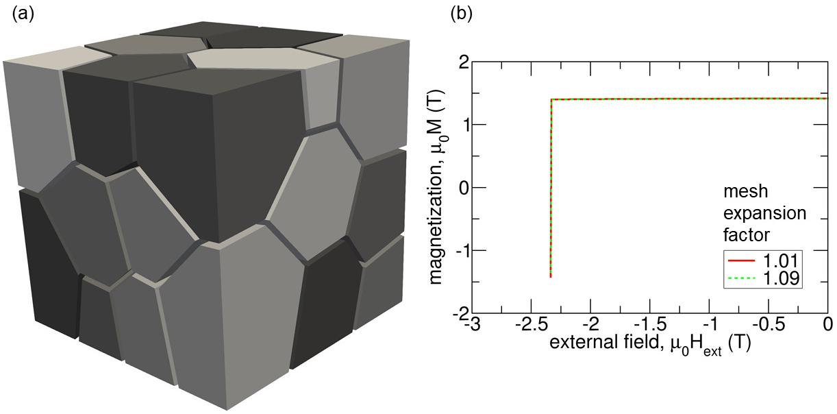
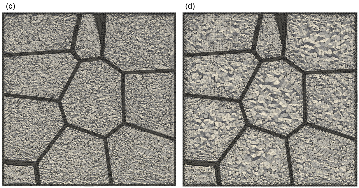
Figure 9: (a) Polycrystalline model of a Nd₂Fe₁₄B magnet. The edge length of the cube is 300 nm. (b) The computed demagnetization curve is the same for (c) an almost uniform mesh ($a=1.01$) and (d) a geometric mesh with expansion factor $a=1.09$.

Computer programs for the semi-automatic generation of synthetic structures are essential to study the influence of the microstructure on the hysteresis properties of permanent magnets. Microstructure features that need to be taken into account are the properties of the grain boundary phase [104, 36, 105], anisotropy enhancement by grain boundary diffusion [86, 53, 106, 107, 57, 108], and the shape of the grains [109, 12, 110, 16, 107]. The grain boundary properties may be anisotropic based on the orientation of the grain boundary with respect to the anisotropy direction [37, 111, 112].

Software tools for the generation of synthetic microstructures include Neper [34] and Dream3d [113]. They generate synthetic granular microstructures with given characteristics such as grain size, grain sphericity, and grain aspect ratio based on Voronoi tessellation [114]. The grain structure has to be modified further, in order to include grain boundary phases. Additional shells around the grains with modified intrinsic magnetic properties may be required in order to represent soft magnetic defect layers or grain boundary diffusion. These modifications of the grain structure can be achieved using computer aided design tools such as Salome [115]. In particular, boundary phases of a specified thickness can be introduced by moving the grain surfaces by a fixed distance along their surface normal. When the finite element method is used for computing the magnetostatic potential, the magnet has to be embedded within an air box. The external mesh is required to treat the boundary conditions at infinity. As a rule of thumb the problem domain surrounding the magnet should have at least 10 times the extension of the magnet [116]. The polyhedral geometry, the grain boundary phase, and the air box that surrounds the magnet are then meshed using a tetrahedral mesh generator. Public domain software packages for mesh generation include NETGEN [117], Gmsh [118], and TetGen [119]. Ott et al. [120] and Fischbacher et al. [14] used NETGEN for meshing nanowires with various tip shape and for meshing polyhedral NdFe₁₂ based magnets. Zighem et al. [121] and Liu et al [122] used Gmsh to mesh complex shaped Co-nanorods and to mesh polyhedral models for Cerium substituted NdFeB magnets, respectively. Fischbacher et al. [107] used TetGen to mesh polyhedral core-shell grains separated by a grain boundary phase.

Figure 9a shows a synthetic grain structure created with Neper [34]. The grain size follows a log-normal distribution. The edge length of the cube containing the 27 grains is 300 nm. The thickness of the grain boundary phase is 6 nm. The material parameters for the main phase and the grain boundary phase were the same as used previously. Figure 9c and 9d show slices through the tetrahedral mesh of the magnet.

In both cases the mesh size at the boundary is 2.7 nm. In (c) an almost uniform mesh ($a=1.01$) was created with an average edge length of 2.9 nm and a maximum of 6 nm in the center of the grains. The number of elements in the magnet is 11.8 millions. In (d) a graded mesh with an expansion factor of 1.09 was created. The average mesh size is then 3.3 nm with a maximum of 11.6 nm. The number of elements is reduced by almost 42 percent to 6.9 million elements. For both meshes we obtain identical demagnetization curves shown in figure 9b. For the preconditioned conjugate gradient [123] used in this study, the time to solution scales linearly with the problem size. Thus the use of geometric meshes reduces the computation time by a factor of 1/2.

3 Rare-earth efficient permanent magnets

3.1 Shape enhanced coercivity

Shape-anisotropy based permanent magnets have a long history. AlNiCo permanent magnets contain elongated particles that form by phase separation during fabrication [124, 125, 126]. AlNiCo magnets were usurped as the magnets with the highest energy density product before the development of permanent magnets based on high uniaxial magnetocrystalline anisotropy; first ferrite magnets and then those based on rare earths [124]. In fact, some have suggested that the development of iron-rare-earth magnets was initially motivated by the perceived need to replace Co, at that time considered strategic and critical [127]. If true, this situation ironically mirrors our current plight. Today shape-anisotropy magnets are again sought as candidates for rare-earth free magnets.

Livingston [125] and Ke et al. [54] discussed the coercivity mechanisms of shape-anisotropy based permanent magnets. In ellipsoidal particles the demagnetizing field is uniform. If the particles are small enough to reverse by uniform rotation [128] the change of the demagnetizing field with the orientation of the magnet leads to an effective uniaxial anisotropy $K_{\mathrm{d}}=(\mu_{0}/2)M_{\mathrm{s}}^{2}(N_{\perp}-N_{\parallel})$ [78], whereby $N_{\perp}$ and $N_{\parallel}$ are the demagnetizing factors perpendicular and normal to the long axis of the ellipsoid. However, if the particle diameter becomes too large magnetization reversal will be non-uniform and coercivity drops [125]. Coercivity also decreases with increased packing density of the particles [129].

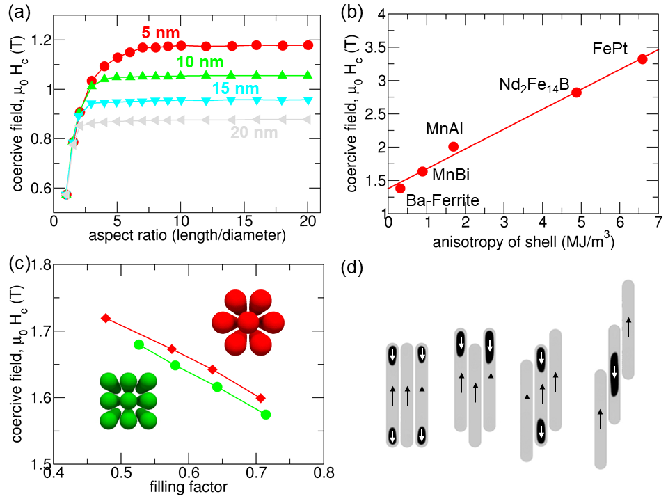
Figure 10: (a) Coercive field as function of the aspect ratio of a Co nanorod for different diameters. (b) Coercive field of a Co wire with an aspect ratio of 10:1 and a diameter of 10 nm as a function of the magnetocrystalline anisotropy of a hard magnetic shell. (c) Reduction of the nucleation field of FePt-coated Co nanorods as function of packing density. (d) Formation of reversed domains in three interacting FePt-coated Co nanorods depending on their relative position.

3.1.1 Magnetic nanowires

High aspect ratio Co, Fe, or CoFe nanowires can be grown via a chemical nanosynthesis polyol process or electrodeposition [130, 131, 132, 133]. Key microstructural features of nanowires and nanowire arrays such as particle shape [120], packing density and alignment [134, 135, 54], and particle coating [135] have been studied using micromagnetic simulations.

The shape of the ends of magnetic nanowires affects the coercivity. An improvement in the coercive field of between 5 and 10 percent is found when the ends are rounded, as opposed to being flattened like an ideal cylinder [130, 134]. This enhancement of the coercive field is due to the reduction of high demagnetizing fields which occur at the front plane of the cylinder [136]. One of the important results from the shape anisotropy work is that the width of elongated nanoparticles is more crucial than the length. Assuming that a particular aspect ratio of 5:1 has been reached, increasing the length will give no further increase in coercive field. Figure 10a gives the computed coercive field of Co cylinders ($K=0.45$ MJ/m³, $\mu_{0}M_{\mathrm{s}}=1.76$ T, $A=1.3$ J/m) with rounded ends as function of the aspect ratio for different cylinder diameters. The smaller the diameter the higher is the coercive field. Ener et al. [133] measured the coercive field of Co-nanorods for diameters of 28 nm, 20 nm, and 11 nm to be 0.36 T/$\mu_{0}$, 0.47 T/$\mu_{0}$, 0.61 T/$\mu_{0}$, respectively. When comparing with micromagnetic simulations we have to consider misorientation, magnetostatic interactions, and thermal activation which occur in the sample but are not taken into account in the results presented in figure 10a. Viau et al. [137] measured a coercive field of 0.9 T/$\mu_{0}$ at $T=140$ K for Co wires with a diameter of 12.5 nm.

3.1.2 Nanowires with core-shell structure

The coercivity of Fe nanorods can be improved by adding anti-ferromagnetic capping layers at the end. Toson et al. [135] showed that exchange bias between the antiferromagnet caps and the Fe rods mitigates the effect of the strong demagnetizing fields and thus increases the coercive field by up to 25 percent. Alternatively, a Co cylinder may be coated with a hard magnetic material. Figure 10b shows the coercive fields of a Co-nanorod with a diameter of 10 nm and an aspect ratio of 10:1 which are coated by a 1 nm thick hard magnetic phase. The coercive field increases linearly with the magnetocrystalline anisotropy constant of the shell.

The demagnetizing field of one rod reduces the switching field of another rod close-by. The closer the rods, the stronger is this effect. We simulated two bulk magnets consisting of either a hexagonal close-packed (h.c.p.) or a regular 3 x 3 arrangement of Co/FePt core-shell rods. As the filling factor increases, the separation of the nanorods becomes smaller, meaning that the demagnetizing effects on neighboring rods increase, so the nucleation field leading to reversal is reduced (see figure 10c). Depending on the arrangement of the nanorods, the magnetostatic interaction field nucleates reversal in neighboring nanowires (see figure 10d). The reversed regions start to grow in the core of the wire owing to the hard magnetic shell.

3.2 Grain boundary engineering

There is evidence from both micromagnetic simulations [138, 86, 106] and experiments [106] that magnetization reversal in conventional magnets starts from the surface of the magnet or the grain boundary. An obvious cure to improve the coercivity of NdFeB magnets is local enhancement of the anisotropy field near the grain surface [86]. This may be achieved by adding heavy rare-earth elements such as Dy in a way that (Dy,Nd)₂Fe₁₄B forms only near the grain boundaries, creating a hard shell-like layer. Possible routes for the latter process are the addition of Dy₂O₃ as a sintering element [139] or by grain boundary diffusion [140, 141]. These production techniques reduce the share of heavy rare-earth elements while maintaining the high coercive field of (Dy,Nd)₂Fe₁₄B magnets. In addition, grain boundary diffused magnets show a higher remanence, because the volume fraction of the (Dy,Nd)₂Fe₁₄B phase, which has a lower magnetization than Nd₂Fe₁₄B, is small. Similarly, the coercive field has been enhanced by Nd-Cu grain boundary diffusion which reduced the Fe content in the grain boundaries [104].

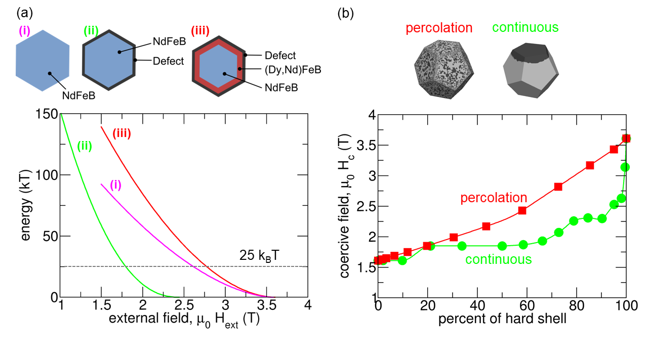
Figure 11: (a) Energy barrier for magnetization reversal as function of the applied field for (i) a perfect Nd₂Fe₁₄B grain, (ii) a Nd₂Fe₁₄B grain with a surface defect with zero anisotropy, and (iii) a system with a defect and a (Dy₄₇Nd₅₃)₂Fe₁₄B shell. The critical field value at which the energy barrier becomes $25k_{\mathrm{B}}$ is the temperature dependent coercive field. $T=450$ K. Data taken from [38]. (b) Coercivity of a Nd₂Fe₁₄B particle as function of the percentage of coverage with a Tb-containing shell for the continuous coverage model and the percolation model.

3.2.1 Core-shell grains

We used the string method [84, 86] to compute the temperature-dependent hysteresis properties of Nd₂Fe₁₄B permanent magnets in order to assess the influence of a soft outer defect and a hard shell created by Dy diffusion. Dodecahedral grain models, approximating the polyhedral geometries of grains observed in actual rare earth permanent magnets, are prepared in three varieties: (i) a pure NdFeB ($K=2.1$ MJ/m³, $\mu_{0}M_{\mathrm{s}}=1.3$ T, $A=4.9$ pJ/m) grain with no defect and no shell, (ii) a NdFeB core with a soft outer defect ($K=0$) of 2 nm thickness and (iii) a Nd₂Fe₁₄B core with a (Dy₄₇Nd₅₃)₂Fe₁₄B hard shell ($K=2.7$ MJ/m³, $\mu_{0}M_{\mathrm{s}}=1$ T, $A=6.4$ pJ/m) of 4 nm plus an outer defect (2nm). The outer grain diameter is constant at 50 nm. Figure 11a shows how the energy barrier decreases as a function of applied field. In all model variations, at $T=450$ K the thermal activation reduces the coercivity by around 25 percent. The reduction in coercivity from the soft defect in (ii) is canceled out by the hard shell in (iii).

In a real magnet the diffusion shell will not necessarily be of uniform thickness or fully cover the grain. We investigate this effect for a Nd₂Fe₁₄B grain with a diameter of 250 nm and a Tb-containing shell. In order to investigate the effects of imperfect shells we simulate systems where parts of the material in a 20 nm thick shell are replaced with the core material, in order to calculate the change in coercive field. A number of approaches are possible. First, a continuous island of varying size is formed where the (Tb_0.5Nd_0.5)₂Fe₁₄B is replaced by Nd₂Fe₁₄B. A 2 nm outer defect layer is still present, with material properties of elements matching those of the material they cover, except that $K=0$. A second approach for an imperfect hard magnetic shell is percolation. Random shell elements are switched to the core material. In the beginning the islands with the core materials are very small until the number of switched elements increase and the islands join up. Depending on the type of the Tb-containing shell the behavior is different. The coercive field is plotted against the percentage of Tb-containing material in the shell in figure 11b for continuous coverage and for percolated coverage. For the continuous coverage model there is an exponential relationship, with a more complete covering leading to the highest coercivity values. As soon as the covering is reduced, the coercivity drops rapidly. The trend is not smooth since at various points the growing island’s boundary reaches the edges and corners of the dodecahedral grain, locations of importance where reversal begins. For the percolation model the coercive field increases linearly with the amount of (Tb,Nd)₂Fe₁₄B in the shell.

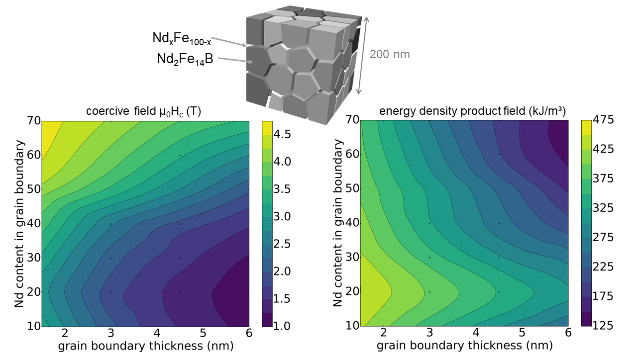
Figure 12: Coercive field (left) and energy density product (right) as function of the grain boundary properties for a nanocrystalline magnet with a grain size of 50 nm. The computed demagnetization curves are corrected with a demagnetizing factor of $N=1/3$. The coercive field is given with respect to the internal field $H$.

3.2.2 Grain boundary properties

By NdCu diffusion high performance Nd₂Fe₁₄B magnets without any heavy rare earths can be achieved [142, 105]. Energy-dispersive X-ray spectroscopy and atom probe analysis [104] showed the formation of a Nd-rich intergranular phase upon infiltration. The Nd rich grain boundary phase predominantly forms at the grain surfaces perpendicular to the anisotropy axes [104]. The coercive field of hot deformed NdFeB magnets increases from 1.5 T/$\mu_{0}$ to 2.3 T/$\mu_{0}$ by Nd-Cu infiltration. Infiltration increases the Nd concentration from 38 at.% to 80 at.% in grain boundary perpendicular to the anisotropy axes, whereas the Nd content in grain boundaries parallel to the anisotropy axes remains low reaching only 25 at.% after infiltration.

In order to understand the influence of the grain boundary properties on coercivity and energy density product we compute demagnetization curves of a nanocrystalline magnet. We vary the thickness of the grain boundary from 1.5 nm to 6 nm, keeping the size of the magnet constant. We also change the Nd content of the grain boundary phase and adjust the magnetization and the exchange constant of the grain boundary phase according to the data published by Sakuma et al. [102]. Please note that the magnetization of Nd_xFe_100-x shows a maximum at $x=20$. We correct the demagnetization curve with the macroscopic demagnetization factor $N=1/3$ and extract the coercive field and the energy density product (see figure 12). Clearly the maximum coercive field is reached for a thin Nd-rich grain boundary phase. For nanocrystalline grains the magnetization of the grain boundary phase contributes to the total magnetization. Therefore, the maximum energy density product occurs for a Nd content of 20 percent and a grain boundary thickness of 1.5 nm. A similar result was reported by Lee et al. [143] who simulated the hysteresis properties as a function of the magnetization and the exchange constant in the grain boundary phase.

3.3 Alternative hard magnetic compounds

In the following we describe how coercive field, remanence, and energy density product change with typical microstructural features for several possible alternative hard magnetic phases.

For all simulations we assume aligned grains. The alignment factor $f=\cos(\phi)$ is always close to unity. Here $\phi$ is the average misalignment angle. To account for higher misalignment the $M_{\mathrm{r}}$-values and the $(BH)_{\mathrm{max}}$-values need to be multiplied with $f$ and $f^{2}$, respectively. Let us consider the following example: The simulated values are $\mu_{0}M_{\mathrm{r}}=1.22$ T and $(BH)_{\mathrm{max}}=251$ kJ/m³ for a L1₀ FeNi magnet. Assuming $\phi=20$ degrees the expected values for the remanence and the energy density products are $\mu_{0}M_{\mathrm{r}}=1.15$ T and $BH_{\mathrm{max}}=222$ kJ/m³.

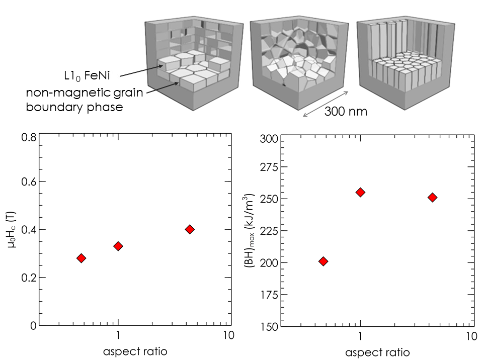
Figure 13: Magnetic properties as function of the aspect ratio of the grains in a L1₀-FeNi granular system with $K=0.35$ MJ/m³. Top: Nanostructures with different aspect ratios of the grains. Left: Coercivity. Right: Energy density product. The computed demagnetization curves are corrected with a demagnetizing factor of $N=1/3$. The coercive field is given with respect to the internal field $H$. Data taken from [110].

3.3.1 L1₀-FeNi based permanent magnets

The rare-earth free FeNi with a tetragonal L1₀ structure has a large saturation magnetization of $\mu_{0}M_{\mathrm{s}}=1.5$ T, which translates to a theoretically possible energy product of $(BH)_{\mathrm{max}}=448$ kJ/m³. However, such a high energy density product requires a sufficiently large magnetocrystalline anisotropy. The empirical law $\kappa>1$ suggests an anisotropy constant $K>1.8$ MJ/m³. Lewis and co-workers [144, 145] studied the crystal lattice, microstructure and magnetic properties of the meteorite NWA 6259. Its L1₀-FeNi phase is highly ordered and therefore regarded as a possible candidate for use in permanent magnets. They estimated the magneto-crystalline anisotropy of the meteorite to be $K=0.84$ MJ/m³. Edström et al. [146] predicted an anisotropy in the range of 0.48 MJ/m³ to 0.77 MJ/m³, using density functional theory. The magnetocrystalline anisotropy linearly depends on the chemical order parameter [147].

Whereas chemical ordering is much smaller in most other attempts to fabricate L1₀ FeNi [148], Goto et al. [149] synthesized L1₀FeNi powder with a degree of order of 0.7 through nitrogen insertion and topotactic extraction. They measured a coercive field of 0.18 T/$\mu_{0}$.

We investigated how nanostructuring may help to create reasonable hard magnetic properties with a low-anisotropy L1₀-FeNi phase. In L1₀-FeNi thin films made by combinatorial sputtering an anisotropy constant $K=0.35$ MJ/m³ was measured by ferromagnetic resonance [110]. We computed the demagnetization curves for three different nanostructures consisting of platelets, equiaxed grains, and columnar grains. The grains have approximately the same volume of $72\times 72\times 34$ nm³, $56\times 56\times 56$ nm³, and $34\times 34\times 146$ nm³, for the platelets, polyhedra, and columns, respectively. The macroscopic shape of the magnet is cubical with an edge length of 300 nm. The volume fraction of the non-magnetic grain boundary phase is 18 percent.

The coercive field increases with increasing aspect ratio. The data summarized in figure 13 shows that the coercivity can be tuned by 120 mT/$\mu_{0}$ through a change in the shape of the grains. The grain shape has no influence on the remanent magnetization which was computed to be $\mu_{0}M_{\mathrm{r}}=1.21$ T. For platelet-shaped grains the energy density product is coercivity limited with $(BH)_{\mathrm{max}}=201$ kJ/m³. For higher coercivity such as in equiaxed and columnar grains the expected energy density product is close to $(BH)_{\mathrm{max}}=255$ kJ/m³.

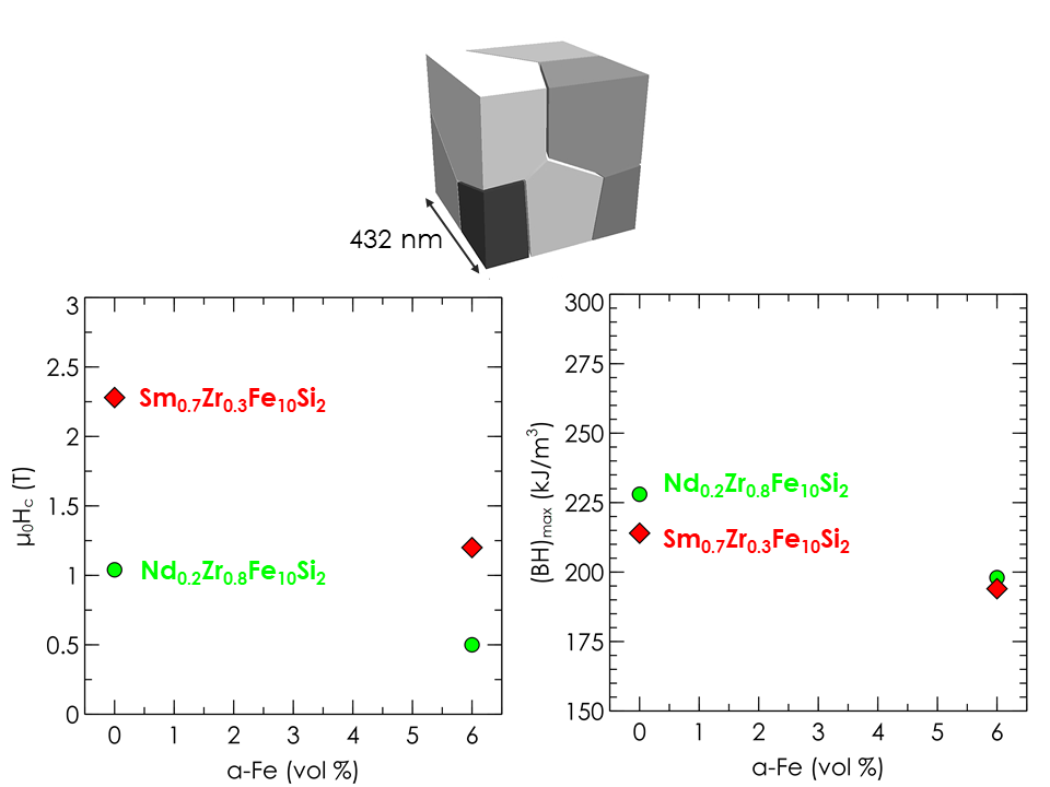
Figure 14: Magnetic properties of Nd_0.2Zr_0.8Fe₁₀Si₂ and Sm_0.7Zr_0.3Fe₁₀Si₂ without and with $\alpha$-Fe inclusions.Top: Granular structure used for the simulation. Left: Coercivity. Right: Energy density product. The computed demagnetization curves are corrected with a demagnetizing factor of $N=1/3$. The coercive field is given with respect to the internal field $H$.

3.3.2 ThMn₁₂ based permanent magnets

Possible candidate phases are NdFe or SmFe compounds in the ThMn₁₂ structure, which were discussed already in the late 1980s [150, 151]. However, NdFe₁₂ and SmFe₁₂ are not stable without any stabilizing elements such as Ti, Mo, Si, or V [152, 153]. At 450 K Nd and Sm based magnetic phases in the ThMn₁₂ structure show a higher magnetization and a higher anisotropy field than Nd₂Fe₁₄B [154, 155]. In addition, the rare earth to transition metal ratio of the 1:12 based magnets is lower. Therefore, magnets based on this phase are considered as a possible alternative to Nd₂Fe₁₄B magnets [87, 156]. The rare-earth content is further reduced if some Nd or Sm is partially replaced with Zr [156]. The fabrication of a magnets in the 1:12 structure is difficult. In contrast to Nd₂Fe₁₄B, phases in the vicinity of R(Fe,M)₁₂ (R rare earth, M stabilizing element) in the equilibrium phase diagram are ferromagnetic. As a consequence there is no isolation of the grains with a non-magnetic or only weakly ferromagnetic grain boundary phase [156]. Gabay and Hadjipanayis [157] measured a coercive field of 1.08 T/$\mu_{0}$ in Sm_0.3Ce_0.3Zr_0.4Fe₁₀Si₂ oriented particles prepared by a mechano-chemical route.

Here we look at the potential of the very rare-earth lean compounds Nd_0.2Zr_0.8Fe₁₀Si₂ [158] and Sm_0.7Zr_0.3Fe₁₀Si₂ [159]. Experiments show that the magnets contain $\alpha$-Fe as a secondary phase with a volume fraction of about 6 percent [158]. Therefore, we investigate the influence of the $\alpha$-Fe content on the hysteresis properties. The synthetic microstructure used for the simulations is shown in figure 14. The volume fraction of the grain boundary phase is 8 percent. The grain boundary phase was assumed to be moderately ferromagnetic with $\mu_{0}M_{\mathrm{s}}=0.56$ T and $A=2.5$ pJ/m. Nd_0.2Zr_0.8Fe₁₀Si₂ shows uniaxial anisotropy [158] with an anisotropy constant of $K=1.16$ MJ/m³ and magnetization of $\mu_{0}M_{\mathrm{s}}=1.12$ T [158]. For Sm_0.7Zr_0.3Fe₁₀Si₂ we use $K=3.5$ MJ/m³ and $\mu_{0}M_{\mathrm{s}}=1.08$ T [159]. We compare two scenarios: (i) A sample without any $\alpha$-Fe as secondary phase, and (ii) a sample in which each grain contains an $\alpha$-Fe inclusion so that the total volume fraction of $\alpha$-Fe is 6 percent.

The presence of $\alpha$-Fe reduces the coercive field. In Nd_0.2Zr_0.8Fe₁₀Si₂ it decreases by about a factor of 1/2 from $\mu_{0}H_{\mathrm{c}}=1.04$ T to $\mu_{0}H_{\mathrm{c}}=0.5$ T. Similarly, in Sm_0.7Zr_0.3Fe₁₀Si₂ the coercive field changes from $\mu_{0}H_{\mathrm{c}}=2.28$ T to $\mu_{0}H_{\mathrm{c}}=1.2$ T when $\alpha$-Fe inclusions are taken into account. The remanent magnetization for the Nd and Sm compound is $\mu_{0}M_{\mathrm{r}}=1.07$ T and $\mu_{0}M_{\mathrm{r}}=1.04$ T, respectively. The presence of $\alpha$-Fe reduces the remanent magnetization by 4 percent and 3 percent in the Nd and the Sm magnet, respectively. With $\alpha$-Fe the energy density product reduces from 228 kJ/m³ to 198 kJ/m³ and from 214 kJ/m³ to 194 kJ/m³ in Nd_0.2Zr_0.8Fe₁₀Si₂ and Sm_0.7Zr_0.3Fe₁₀Si₂, respectively.

4 Summary

Hard magnetic phases for rare-earth free or rare-earth reduced permanent magnets may show a lower magnetocrystalline anisotropy than Nd₂Fe₁₄B. Therefore a detailed understanding of the influence of the microstructure on the magnetic properties is of utmost importance for the development of new permanent magnets. Computational micromagnetics reveals the main microstructural effects on the coercive field, the remanence, and the energy density product.

4.1 Grain boundary phase

The grain boundary phase significantly influences the coercive field. If the grain boundary phase is ferromagnetic, the coercive field decreases with increasing thickness of the grain boundary. Dy or Tb diffusion recovers the coercivity of magnets with ferromagnetic grain boundary phases. A heavy rare-earth containing shell with a thickness of 10 nm doubles the coercive field which keeps increasing moderately with further increasing thickness of the hard magnetic shell. High energy products and reasonable coercive fields can be achieved for ferromagnetic grain boundaries with thicknesses below 3 nm. In nanocrystalline magnets the remanence and energy density product increase with increasing magnetization of the grain boundary phase.

4.2 Grain shape

In magnets based on CoFe nanorods coercivity is mostly governed by the thickness of the rods. The highest coercive fields can be obtained if the rod diameter is comparable with the exchange length of the material. Nanostructuring is essential and helps to improve the hysteresis loop squareness in materials with low magnetocrystalline anisotropy. For the magnetic properties of commonly synthesized L1₀ FeNi the energy product is coercivity limited. A change from platelet-shaped grains to columnar grains may increase the energy density product by 25 percent.

4.3 Soft magnetic secondary phases

Soft magnetic inclusions may reduce the coercive field by up to a factor of 1/2. If the magnetocrystalline anisotropy is sufficiently high, such as in SmFe or NdFe compounds in the ThMn₁₂ structure, still excellent hard magnetic properties can be achieved despite the presence of $\alpha$-Fe. The reduction of the energy density product by soft magnetic inclusions is about 10 percent.

5 Conclusion

The coercivity and the energy density product were computed for several rare-earth reduced and rare-earth free permanent magnets using micromagnetic simulations. For some materials the theoretically predicted values are higher than those currently achieved in experiments. This discrepancy emphasizes the importance of the microstructure. A small grain size, thin non-magnetic grain boundary phases that separate the grains, and elongated grains for phases with low magnetocrystalline anisotropy are essential to achieve a high coercive field.

References

References

- [1] Sagawa M, Fujimura S, Togawa N, Yamamoto H and Matsuura Y 1984 J. Appl. Phys. 55 2083–2087
- [2] Croat J J, Herbst J F, Lee R W and Pinkerton F E 1984 J. Appl. Phys. 55 2078–2082
- [3] Constantinides S 2016 Magnetics Magazine Spring 2016 6
- [4] Yang Y, Walton A, Sheridan R, Güth K, Gauß R, Gutfleisch O, Buchert M, Steenari B M, Van Gerven T, Jones P T et al. 2017 J. Sustain. Metall. 3 122–149
- [5] Coey J M D 2010 Magnetism and Magnetic Materials (Cambridge University Press)
- [6] Sprecher B, Daigo I, Spekkink W, Vos M, Kleijn R, Murakami S and Kramer G J 2017 Environ. Sci. Technol. 51 3860–3870
- [7] Sander D, Valenzuela S, Makarov D, Marrows C, Fullerton E, Fischer P, McCord J, Vavassori P, Mangin S, Pirro P, Hillebrands B, Kent A, Jungwirth T, Gutfleisch O, Kim C and Berger A 2017 J. Phys. D Appl. Phys. 50 363001
- [8] King A H, Eggert R G and Gschneidner K A 2016 Handbook on the Physics and Chemistry of Rare Earths 50 19–46
- [9] Coey J 2012 Scripta Mater. 67 524–529
- [10] Nakamura H 2017 Scripta Mater. (Preprint https://doi.org/10.1016/j.scriptamat.2017.11.010)
- [11] Exl L, Bance S, Reichel F, Schrefl T, Stimming H P and Mauser N J 2014 J. Appl. Phys. 115 17D118
- [12] Sepehri-Amin H, Ohkubo T and Hono K 2016 Mater. Trans. 57 1221–1229
- [13] Tsukahara H, Lee S J, Iwano K, Inami N, Ishikawa T, Mitsumata C, Yanagihara H, Kita E and Ono K 2016 AIP Adv. 6 056405
- [14] Fischbacher J, Kovacs A, Oezelt H, Schrefl T, Exl L, Fidler J, Suess D, Sakuma N, Yano M, Kato A et al. 2017 AIP Adv. 7 045310
- [15] Tanaka T, Furuya A, Uehara Y, Shimizu K, Fujisaki J, Ataka T and Oshima H 2017 IEEE Trans. Magn.
- [16] Erokhin S and Berkov D 2017 Phys. Rev. Appl 7 014011
- [17] Sagawa M, Hirosawa S, Tokuhara K, Yamamoto H, Fujimura S, Tsubokawa Y and Shimizu R 1987 J. Appl. Phys. 61 3559–3561
- [18] Brown Jr W 1962 Magnetostatic principles in ferromagnetism. series of monographs on selected topicss in solid state physics
- [19] Fidler J 1997 Review of bulk permanent magnets Magnetic Hysteresis in Novel Magnetic Materials ed Hadjipanayis G C (Dordrecht: Springer) pp 567–597
- [20] Buschow K H J, Boer F R et al. 2003 Physics of magnetism and magnetic materials vol 92 (Springer)
- [21] Skomski R and Coey J 2016 Scr. Mater. 112 3–8
- [22] Sato M and Ishii Y 1989 J. Appl. Phys. 66 983–985
- [23] Brown Jr W F 1957 Phys. Rev. 105 1479
- [24] Thiele A 1970 J. Appl. Phys. 41 1139–1145
- [25] Slonczewski J, Malozemoff A and Voegeli O 1973 AIP Conf. Proc. 10 458–477
- [26] Brown Jr W F 1945 Rev. Mod. Phys. 17 15
- [27] Shtrikman S and Treves D 1960 J. Appl. Phys. 31 S72–S73
- [28] Coey J 1995 J. Korean Magn. Soc. 5 399–403
- [29] Kronmüller H and Fähnle M 2003 Micromagnetism and the microstructure of ferromagnetic solids. Cambridge university press
- [30] Fischbacher J, Kovacs A, Oezelt H, Gusenbauer M, Schrefl T, Exl L, Givord D, Dempsey N, Zimanyi G, Winklhofer M et al. 2017 Appl. Phys. Lett. 111 072404
- [31] Kronmüller H, Durst K D and Sagawa M 1988 J. Magn. Magn. Mater. 74 291–302
- [32] Grönefeld M and Kronmüller H 1989 J. Magn. Magn. Mater. 80 223–228
- [33] Givord D, Tenaud P and Viadieu T 1988 IEEE Trans. Magn. 24 1921
- [34] Quey R, Dawson P and Barbe F 2011 Comput. Methods Appl. Mech. Eng. 200 1729
- [35] Murakami Y, Tanigaki T, Sasaki T, Takeno Y, Park H, Matsuda T, Ohkubo T, Hono K and Shindo D 2014 Acta Mater. 71 370–379
- [36] Zickler G A, Toson P, Asali A and Fidler J 2015 Phys. Procedia 75 1442–1449
- [37] Zickler G A, Fidler J, Bernardi J, Schrefl T and Asali A 2017 Adv. Mater. Sci. Eng. 2017
- [38] Bance S, Fischbacher J, Kovacs A, Oezelt H, Reichel F and Schrefl T 2015 JOM 67 1350–1356
- [39] Brown W F 1959 J. phys. radium 20 101–104
- [40] Jackson J D 1998 Classical Electrodynamics (New York: Wiley)
- [41] Kinderlehrer D and Ma L 1997 J. Nonlinear Sci. 7 101–128
- [42] Cullity B D and Graham C D 2011 Introduction to magnetic materials (John Wiley & Sons)
- [43] Fidler J and Schrefl T 2000 J. Phys. D: Appl. Phys. 33 R135
- [44] Sun J and Monk P 2006 IEEE Trans. Magn. 42 1643–1647
- [45] Shepherd D, Miles J, Heil M and Mihajlović M 2014 IEEE Trans. Magn. 50 1–4
- [46] Aharoni A 2000 Introduction to the Theory of Ferromagnetism vol 109 (Clarendon Press)
- [47] Fabian K, Kirchner A, Williams W, Heider F, Leibl T and Huber A 1996 Geophys. J. Int. 124 89–104
- [48] Schabes M and Aharoni A 1987 IEEE Trans. Magn. 23 3882–3888
- [49] Nakatani Y, Uesaka Y and Hayashi N 1989 Japanese Journal of Applied Physics 28 2485
- [50] Pavel C C, Lacal-Arántegui R, Marmier A, Schüler D, Tzimas E, Buchert M, Jenseit W and Blagoeva D 2017 Resources Policy 52 349–357
- [51] Dorrell D G, Knight A M, Popescu M, Evans L and Staton D A 2010 Comparison of different motor design drives for hybrid electric vehicles Energy Conversion Congress and Exposition (ECCE), 2010 IEEE (IEEE) pp 3352–3359
- [52] Furuya A, Fujisaki J, Shimizu K, Uehara Y, Ataka T, Tanaka T and Oshima H 2015 IEEE Trans. Magn. 51 1–4
- [53] Oikawa T, Yokota H, Ohkubo T and Hono K 2016 AIP Adv. 6 056006
- [54] Ke L, Skomski R, Hoffmann T D, Zhou L, Tang W, Johnson D D, Kramer M J, Anderson I E and Wang C Z 2017 Appl. Phys. Lett. 111 022403
- [55] Sepehri-Amin H, Thielsch J, Fischbacher J, Ohkubo T, Schrefl T, Gutfleisch O and Hono K 2017 Acta Mater. 126 1–10
- [56] Soderžnik M, Sepehri-Amin H, Sasaki T, Ohkubo T, Takada Y, Sato T, Kaneko Y, Kato A, Schrefl T and Hono K 2017 Acta Mater.
- [57] Tang X, Sepehri-Amin H, Ohkubo T, Yano M, Ito M, Kato A, Sakuma N, Shoji T, Schrefl T and Hono K 2018 Acta Mater. 144 884–895
- [58] Moré J J and Thuente D J 1994 ACM Trans. Math. Softw. 20 286–307
- [59] Koehler T and Fredkin D 1992 IEEE Transactions on magnetics 28 1239–1244
- [60] Barzilai J and Borwein J M 1988 IMA J. Numer. Anal. 8 141–148
- [61] Abert C, Wautischer G, Bruckner F, Satz A and Suess D 2014 J. Appl. Phys. 116 123908
- [62] Vansteenkiste A, Leliaert J, Dvornik M, Helsen M, Garcia-Sanchez F and Van Waeyenberge B 2014 Aip Adv. 4 107133
- [63] Alouges F 1997 SIAM J. Numer. Anal. 34 1708–1726
- [64] Bartels S 2005 SSIAM J. Numer. Anal. 43 220–238
- [65] Cohen R, Lin S Y and Luskin M 1989 Comput. Phys. Commun. 53 455–465
- [66] Tsukahara H, Iwano K, Mitsumata C, Ishikawa T and Ono K 2017 AIP Adv. 7 056224
- [67] Goldfarb D, Wen Z and Yin W 2009 SIAM J. Imag. Sci. 2 84–109
- [68] Landau L and Lifshitz E 1935 Phys. Z. Sowjetunion 8 101–114
- [69] Gill P E, Murray W and Wright M H 1981 Practical optimization (Academic press)
- [70] Gilbert T 1955 Phys. Rev. 100 1243
- [71] Mallinson J 1987 IEEE Trans. Magn. 23 2003–2004
- [72] Tsukahara H, Iwano K, Mitsumata C, Ishikawa T and Ono K 2017 AIP Adv. 7 056234
- [73] Fu S, Cui W, Hu M, Chang R, Donahue M J and Lomakin V 2016 IEEE Trans. Magn. 52 1–9
- [74] Fangohr H, Albert M and Franchin M 2016 Nmag micromagnetic simulation tool—software engineering lessons learned Software Engineering for Science (SE4Science), IEEE/ACM International Workshop on (IEEE) pp 1–7
- [75] Scholz W, Fidler J, Schrefl T, Suess D, Forster H, Tsiantos V et al. 2003 Comput. Mater. Sci. 28 366–383
- [76] Schabes M E 1991 J. Magn. Magn. Mater. 95 249–288
- [77] Gaunt P 1976 Philos. Mag. 34 775–780
- [78] Kronmüller H, Durst K D and Martinek G 1987 J. Magn. Magn. Mater. 69 149–157
- [79] Givord D, Rossignol M and Taylor D 1992 J. Phys. IV 2 C3–95
- [80] Dittrich R, Schrefl T, Suess D, Scholz W, Forster H and Fidler J 2002 J. Magn. Magn. Mater. 250 12–19
- [81] Weinan E, Ren W and Vanden-Eijnden E 2002 Phys. Rev. B 66 052301
- [82] Henkelman G and Jónsson H 2000 J. Chem. Phys. 113 9978–9985
- [83] Zhang L, Ren W, Samanta A and Du Q 2016 npj Comput. Mater. 2 16003
- [84] Weinan E, Ren W and Vanden-Eijnden E 2007 J. Chem. Phys.
- [85] Carilli M F, Delaney K T and Fredrickson G H 2015 J. Chem. Phys. 143 054105
- [86] Bance S, Fischbacher J and Schrefl T 2015 J. Appl. Phys. 117 17A733
- [87] Hirosawa S, Nishino M and Miyashita S 2017 Adv. Nat. Sci.: Nanosci. Nanotechnol. 8 013002
- [88] Miyashita S, Nishino M, Toga Y, Hinokihara T, Miyake T, Hirosawa S and Sakuma A 2017 Scr. Mater.
- [89] Sharrock M 1994 J. Appl. Phys. 76 6413–6418
- [90] Toga Y, Matsumoto M, Miyashita S, Akai H, Doi S, Miyake T and Sakuma A 2016 Phys. Rev. B 94 174433
- [91] Givord D, Lienard A, Tenaud P and Viadieu T 1987 J. Magn. Magn. Mater. 67 L281–L285
- [92] Villas-Boas V, Gonzalez J, Cebollada F, Rossignol M, Taylor D and Givord D 1998 J. Magn. Magn. Mater. 185 180–186
- [93] Okamoto S, Goto R, Kikuchi N, Kitakami O, Akiya T, Sepehri-Amin H, Ohkubo T, Hono K, Hioki K and Hattori A 2015 J. Appl. Phys. 118 223903
- [94] Schabes M E and Bertram H N 1988 J. Appl. Phys. 64 1347–1357
- [95] Thielsch J, Suess D, Schultz L and Gutfleisch O 2013 J. Appl. Phys. 114 223909
- [96] Skomski R 2008 Simple models of magnetism (Oxford University Press)
- [97] Schmidts H and Kronmüller H 1991 J. Magn. Magn. Mater. 94 220–234
- [98] Bance S, Seebacher B, Schrefl T, Exl L, Winklhofer M, Hrkac G, Zimanyi G, Shoji T, Yano M, Sakuma N et al. 2014 J. Appl. Phys. 116 233903
- [99] Sepehri-Amin H, Ohkubo T, Gruber M, Schrefl T and Hono K 2014 Scr. Mater. 89 29–32
- [100] Liu J, Sepehri-Amin H, Ohkubo T, Hioki K, Hattori A, Schrefl T and Hono K 2015 Acta Mater. 82 336–343
- [101] Yazid M M, Olsen S H and Atkinson G J 2016 IEEE Trans. Magn. 52 1–10
- [102] Sakuma A, Suzuki T, Furuuchi T, Shima T and Hono K 2015 Appl. Phys Express 9 013002
- [103] Szabo B A and Babuška I 1991 Finite element analysis (John Wiley & Sons)
- [104] Sepehri-Amin H, Ohkubo T, Nagashima S, Yano M, Shoji T, Kato A, Schrefl T and Hono K 2013 Acta Mater. 61 6622–6634
- [105] Liu L, Sepehri-Amin H, Ohkubo T, Yano M, Kato A, Shoji T and Hono K 2016 J. Alloys Compd. 666 432–439
- [106] Helbig T, Loewe K, Sawatzki S, Yi M, Xu B X and Gutfleisch O 2017 Acta Mater. 127 498–504
- [107] Fischbacher J, Kovacs A, Exl L, Kühnel J, Mehofer E, Sepehri-Amin H, Ohkubo T, Hono K and Schrefl T 2017 Scr. Mater. (Preprint https://doi.org/10.1016/j.scriptamat.2017.11.020)
- [108] Li W, Zhou Q, Zhao L, Wang Q, Zhong X and Liu Z 2018 J. Magn. Magn. Mater. 451 704–709
- [109] Yi M, Gutfleisch O and Xu B X 2016 J. Appl. Phys. 120 033903
- [110] Kovacs A, Ozelt H, Fischbacher J, Schrefl T, Kaidatzis A, Salikhof R, Farle M, Giannopoulos G and Niarchos D 2017 IEEE Trans. Magn. 53 7002205
- [111] Zickler G A and Fidler J 2017 Adv. Mater. Sci. Eng. 2017 1461835
- [112] Fujisaki J, Furuya A, Uehara Y, Shimizu K, Ataka T, Tanaka T, Oshima H, Ohkubo T, Hirosawa S and Hono K 2016 AIP Adv. 6 056028
- [113] Groeber M A and Jackson M A 2014 Integr. Mater. Manuf. Innov. 3 5
- [114] Schrefl T and Fidler J 1992 J. Magn. Magn. Mater. 111 105–114
- [115] Ribes A and Caremoli C 2007 Salome platform component model for numerical simulation Computer Software and Applications Conference, 2007. COMPSAC 2007. 31st Annual International vol 2 (IEEE) pp 553–564
- [116] Chen Q and Konrad A 1997 IEEE Trans. Magn. 33 663–676
- [117] Schöberl J 1997 Comput. Visual. Sci. 1 41–52
- [118] Geuzaine C and Remacle J F 2009 International journal for numerical methods in engineering 79 1309–1331
- [119] Si H 2015 ACM Trans. Math. Softw. 41 11
- [120] Ott F, Maurer T, Chaboussant G, Soumare Y, Piquemal J Y and Viau G 2009 J. Appl. Phys. 105 013915
- [121] Zighem F and Mercone S 2014 J. Appl. Phys. 116 193904
- [122] Liu D, Zhao T, Li R, Zhang M, Shang R, Xiong J, Zhang J, Sun J and Shen B 2017 AIP Adv. 7 056201
- [123] Exl L, Fischbacher J, Kovacs A, Oezelt H, Gusenbauer M and Schrefl T 2018 arXiv preprint arXiv:1801.03690
- [124] Becker J 1968 IEEE Trans. Magn. 4 239–249
- [125] Livingston J 1981 J. Appl. Phys. 52 2544–2548
- [126] Jimenez-Villacorta F and Lewis L H 2014 Advanced permanent magnetic materials Nanomagnetism ed Gonzalez Estevez J M (One Central Press)
- [127] Hadjipanayis G C, Hazelton R and Lawless K 1983 Appl. Phys. Lett. 83 797–799
- [128] Frei E, Shtrikman S and Treves D 1957 Phys. Rev. 106 446
- [129] Kittel C 1949 Rev. Mod. Phys. 21 541
- [130] Maurer T, Ott F, Chaboussant G, Soumare Y, Piquemal J and Viau G 2007 Appl. Phys. Lett. 91 172501
- [131] Niarchos D, Giannopoulos G, Gjoka M, Sarafidis C, Psycharis V, Rusz J, Edström A, Eriksson O, Toson P, Fidler J et al. 2015 JOM 67 1318–1328
- [132] Palmero E M, Bran C, del Real R P and Vázquez M 2016 J. Phys. Conf. Ser. 755 012001
- [133] Ener S, Anagnostopoulou E, Dirba I, Lacroix L M, Ott F, Blon T, Piquemal J Y, Skokov K P, Gutfleisch O and Viau G 2018 Acta Mater. 145 290–297
- [134] Bance S, Fischbacher J, Schrefl T, Zins I, Rieger G and Cassignol C 2014 J. Magn. Magn. Mater. 363 121–124
- [135] Toson P, Asali A, Wallisch W, Zickler G and Fidler J 2015 IEEE Trans. Magn. 51 1–4
- [136] Holz A 1968 Phys. Status Solidi b 25 567–582
- [137] Viau G, Garcıa C, Maurer T, Chaboussant G, Ott F, Soumare Y and Piquemal J Y 2009 phys. status solidi (a) 206 663–666
- [138] Bance S, Oezelt H, Schrefl T, Ciuta G, Dempsey N M, Givord D, Winklhofer M, Hrkac G, Zimanyi G, Gutfleisch O et al. 2014 Appl. Phys. Lett. 104 182408
- [139] Ghandehari M H and Fidler J 1987 Mater. Lett. 5 285–288
- [140] Hirota K, Nakamura H, Minowa T and Honshima M 2006 IEEE Trans. Magn. 42 2909–2911
- [141] Soderžnik M, Korent M, Soderžnik K Ž, Katter M, Üstüner K and Kobe S 2016 Acta Mater. 115 278–284
- [142] Akiya T, Liu J, Sepehri-Amin H, Ohkubo T, Hioki K, Hattori A and Hono K 2014 Scr. Mater. 81 48–51
- [143] Lee J H, Choe J, Hwang S and Kim S K 2017 J. Appl. Phys. 122 073901
- [144] Lewis L H, Mubarok A, Poirier E, Bordeaux N, Manchanda P, Kashyap A, Skomski R, Goldstein J, Pinkerton F, Mishra R et al. 2014 J. Phys.: Condens. Matter 26 064213
- [145] Poirier E, Pinkerton F E, Kubic R, Mishra R K, Bordeaux N, Mubarok A, Lewis L H, Goldstein J I, Skomski R and Barmak K 2015 J. Appl. Phys. 117 17E318
- [146] Edström A, Chico J, Jakobsson A, Bergman A and Rusz J 2014 Phys. Rev. B 90 014402
- [147] Kojima T, Mizuguchi M, Koganezawa T, Osaka K, Kotsugi M and Takanashi K 2011 Jpn. J. Appl. Phys. 51 010204
- [148] Takanashi K, Mizuguchi M, Kojima T and Tashiro T 2017 J. Phys. D 50 483002
- [149] Goto S, Kura H, Watanabe E, Hayashi Y, Yanagihara H, Shimada Y, Mizuguchi M, Takanashi K and Kita E 2017 Scientific reports 7 13216
- [150] Buschow K 1988 J. Appl. Phys. 63 3130–3135
- [151] Hu B P, Li H S, Gavigan J and Coey J 1989 J. Phys.: Condens. Matter 1 755
- [152] De Mooij D and Buschow K 1988 J. Less Common Met. 136 207–215
- [153] Ohashi K, Tawara Y, Osugi R and Shimao M 1988 J. Appl. Phys. 64 5714–5716
- [154] Hirayama Y, Takahashi Y, Hirosawa S and Hono K 2015 Scr. Mater. 95 70–72
- [155] Kuno T, Suzuki S, Urushibata K, Kobayashi K, Sakuma N, Yano M, Kato A and Manabe A 2016 AIP Adv. 6 025221
- [156] Gabay A and Hadjipanayis G 2017 Scr. Mater.
- [157] Gabay A and Hadjipanayis G 2017 J. Magn. Magn. Mater. 422 43–48
- [158] Gjoka M, Psycharis V, Devlin E, Niarchos D and Hadjipanayis G 2016 J. Alloys Compd. 687 240–245
- [159] Gabay A, Cabassi R, Fabbrici S, Albertini F and Hadjipanayis G 2016 J. Alloys Compd. 683 271–275