Preservation of dynamics in coupled cavity system using second order nonlinearity

Abstract

We study two coupled cavities with a single two-level system in each and a second-order non-linear process in one of the cavities. Introduction of a harmonic time dependence on the non-linear coupling is utilized for the preservation of dynamics. It is observed that, even though the preservation period is independent of the initial state, the preserved dynamics depends on the initial state. We calculated the von Neumann entropy and mutual information to study the entanglement present between the subsystems. From which it is found that the time-dependent coupling also preserves the entanglement produced in the system.

(Day Month Year)

1 Introduction

Jaynes-Cummings model (JCM) describes the interaction of quantized electromagnetic radiation with a single two-level system (TLS/qubit [1]) in the rotating wave approximation [2]. Over the years JCM has undergone various modifications and has touched different aspects of light-matter physics; including non-linear, deformed and multilevel systems [3, 4, 5]. Tailoring this fundamental interaction is the basis of quantum technologies, like, quantum computers[6], quantum computations[7, 8] and quantum simulations[9, 10]. Various optical schemes have been reported in this regard [11, 12, 13, 14, 15]. Cavity configurations for generation of entanglement [16, 17, 18, 19, 20], preservation of quantum coherence[21, 22, 23], recovery of quantum correlations[24, 25], controlled quantum state transfer [26, 27, 28, 29], quantum state squeezing[30, 31] and ultra strong quantum systems [32] are well reviewed in the literature.

Nonlinear processes are an integral part of experiments in quantum optics[33]. Among which, second order non-linear processes are of special interest in optical squeezing[34] and entangled pair production[35]. Single photon non-linear process has been experimentally reported using 2D materials like graphene nanostructures [36] and dichalcogenide MoS₂[37]. This completely transforms the experimental outlook and realization of quantum states.

In this article, we study the effects of degenerate second order non-linear process[38] on the dynamics of quantum states. Further, the influence of a harmonic time-dependent non-linear coupling is investigated and the emergence of preservation of dynamics with a tunable spontaneous parametric down conversion (SPDC) coupling is shown. The studies were extended to off resonant case.

Measures such as, entropy, concurrence, fidelity etc. can be used to quantify the quantumness of the system [39, 40, 41, 42, 43, 44, 45]. Also, measures like continuous variable synchronization [46, 47] and mutual information [48, 49, 50] can estimate the correlations between the systems. In information theory, mutual information is treated as a measure of entanglement [51]. As the number of subsystems increases, quantifying the correlation between a given pair demands a mutual measure like mutual information. All these measures have been used in various works [52, 53, 54, 55, 56, 57]. Here, we use von Neumann entropy and mutual information for this purpose.

2 Coupled cavities with qubits

We consider two coupled single mode ($\omega_{c}$) optical cavities with a qubit/two-level system (TLS) of level separation $\omega_{a}$ in both. By taking $\hbar=1$, the system can be described by the sum of free Hamiltonian and the interaction Hamiltonian given by [58],

$$\hat{H}_{0}=\sum_{i=1}^{2}\left(\frac{1}{2}\omega_{ai}\sigma_{z}^{(i)}+\omega_{ci}{a_{i}}^{\dagger}a_{i}\right),$$ (1)

and

$$\hat{H}_{I}=J\left({a_{1}}^{\dagger}a_{2}+a_{1}{a_{2}}^{\dagger}\right)+\sum_{i=1}^{2}\lambda_{i}\left({a_{i}}^{\dagger}\sigma_{-}^{(i)}+a_{i}\sigma_{+}^{(i)}\right).$$ (2)

Here, $\lambda_{i}$ is the coupling between photons and qubit in the $i$th cavity and $J$ is the photon hopping factor. The operators $a_{i}$ $(a_{i}^{\dagger})$ is the annihilation (creation) operator of the $i$th cavity mode, $\sigma_{z}^{(i)}$ is the population inversion operator, $\sigma_{+}^{(i)}$ $(\sigma_{-}^{(i)})$ is the raising (lowering) operator of qubits in the $i$th cavity. A general state, of the form $\ket{\psi}=\ket{\mbox{qubit}_{1},\mbox{field}_{1},\mbox{qubit}_{2},\mbox{field}_{2}}$, with a single excitation can be written in the Fock basis as,

$$\ket{\psi(t)}=q_{1}\ket{1000}+f_{1}\ket{0100}+q_{2}\ket{0010}+f_{2}\ket{0001},$$ (3)

where $q_{i}$ and $f_{i}$ are the time-dependent coefficients of qubits and fields respectively. The system can be easily solved for resonant case by solving the Schrödinger equation,

$$i\frac{\partial\ket{\psi}}{\partial t}=\hat{H}\ket{\psi}.$$ (4)

The resulting coupled differential equations are,

$$i\frac{\partial}{\partial t}q_{1}(t) =\lambda f_{1}(t)\,,$$ (5)

$$i\frac{\partial}{\partial t}f_{1}(t) =\lambda q_{1}(t)+Jf_{2}(t)\,,$$ (6)

$$i\frac{\partial}{\partial t}q_{2}(t) =\lambda f_{2}(t)\,,$$ (7)

$$i\frac{\partial}{\partial t}f_{2}(t) =\lambda q_{2}(t)+Jf_{1}(t)\,.$$ (8)

Here, we have taken $\lambda_{i}=\lambda$ and $\omega_{ai}=\omega_{ci}=\omega$. The Eqs. (5)–(8) can be used to obtain the respective Laplace transforms of $q_{1}(t)$, $q_{2}(t)$, $f_{1}(t)$ and $f_{2}(t)$s as,

$$Q_{1}(s)= \frac{-iJ\lambda^{2}q_{2}(0)+J\lambda f_{2}(0)s+i\lambda f_{1}(0)\left(\lambda^{2}+s^{2}\right)}{J^{2}s^{2}+\lambda^{4}+2\lambda^{2}s^{2}+s^{4}}$$ (9)

$$-\frac{q_{1}(0)s\left(J^{2}+\lambda^{2}+s^{2}\right)}{J^{2}s^{2}+\lambda^{4}+2\lambda^{2}s^{2}+s^{4}},$$

$$F_{1}(s)= \frac{J\lambda q_{2}(0)s+iJf_{2}(0)s^{2}+i\lambda q_{1}(0)\left(\lambda^{2}+s^{2}\right)}{J^{2}s^{2}+\lambda^{4}+2\lambda^{2}s^{2}+s^{4}}$$ (10)

$$-\frac{f_{1}(0)s\left(\lambda^{2}+s^{2}\right)}{J^{2}s^{2}+\lambda^{4}+2\lambda^{2}s^{2}+s^{4}},$$

$$Q_{2}(s)= \frac{-iJ\lambda^{2}q_{1}(0)+J\lambda f_{1}(0)s+i\lambda f_{2}(0)\left(\lambda^{2}+s^{2}\right)}{J^{2}s^{2}+\lambda^{4}+2\lambda^{2}s^{2}+s^{4}}$$ (11)

$$-\frac{q_{2}(0)s\left(J^{2}+\lambda^{2}+s^{2}\right)}{J^{2}s^{2}+\lambda^{4}+2\lambda^{2}s^{2}+s^{4}},$$

$$F_{2}(s)= \frac{J\lambda q_{1}(0)s+iJf_{1}(0)s^{2}+i\lambda q_{2}(0)\left(\lambda^{2}+s^{2}\right)}{J^{2}s^{2}+\lambda^{4}+2\lambda^{2}s^{2}+s^{4}}.$$ (12)

$$-\frac{f_{2}(0)s\left(\lambda^{2}+s^{2}\right)}{J^{2}s^{2}+\lambda^{4}+2\lambda^{2}s^{2}+s^{4}}.$$

Now by choosing appropriate initial conditions we can obtain solutions to the Eqs. (5)–(8) by taking the inverse Laplace transform of the Eqs. (9)–(12). For instance, with $\ket{\psi(0)}=\ket{1000}$, we have $q_{1}(0)=1$ and $f_{1}(0)=q_{2}(0)=f_{2}(0)=0$ and the corresponding time evolution of probabilities becomes,

$$|q_{1}(t)|^{2}=\left|\frac{\left[\left(\xi_{+}^{2}+2\lambda^{2}\right)\cosh\left(\frac{t\xi_{-}}{\sqrt{2}}\right)-\left(\xi_{-}^{2}+2\lambda^{2}\right)\cosh\left(\frac{t\xi_{+}}{\sqrt{2}}\right)\right]^{2}}{4(J^{4}+4\lambda^{2}J^{2})}\right|,$$ (13)

$$|q_{2}(t)|^{2}=\left|\frac{\left[\xi_{+}\sinh\left(\frac{t\xi_{-}}{\sqrt{2}}\right)-\xi_{-}\sinh\left(\frac{t\xi_{+}}{\sqrt{2}}\right)\right]^{2}}{2(J^{2}+4\lambda^{2})}\right|,$$ (14)

$$|f_{1}(t)|^{2}= \left|\frac{\lambda^{2}\left[\sinh^{2}\left(\frac{t\xi_{-}}{\sqrt{2}}\right)+\sinh^{2}\left(\frac{t\xi_{+}}{\sqrt{2}}\right)\right]}{J^{2}+4\lambda^{2}}\right.$$ (15)

$$\left.{}+\frac{-\xi_{-}\xi_{+}\sinh\left(\frac{t\xi_{+}}{\sqrt{2}}\right)\sinh\left(\frac{t\xi_{-}}{\sqrt{2}}\right)}{J^{2}+4\lambda^{2}}\right|,$$

$$|f_{2}(t)|^{2}=\left|\frac{\lambda^{2}\left[\cosh\left(\frac{t\xi_{-}}{\sqrt{2}}\right)-\cosh\left(\frac{t\xi_{+}}{\sqrt{2}}\right)\right]^{2}}{J^{2}+4\lambda^{2}}\right|\,.$$ (16)

Where $\xi_{\pm}=\sqrt{-J^{2}-2\lambda^{2}\pm\sqrt{J^{4}+4J^{2}\lambda^{2}}}$. The evolution of the qubits and fields attributes to the state transfer between the coupled cavities. We have studied similar system in our previous work with Kerr medium as a controller[29]. In the following section we introduce a two photon process to the above system.

3 Coupled cavities with qubits and two photon process

Two photon processes are widely used for producing entangled photon pairs through spontaneous parametric down conversion (SPDC)[35] and to produce squeezed light[34]. The experimental realization of single photon SPDC [36, 37] makes it possible to have states with a maximum of one excitation in $\chi^{(2)}$ mode and still shows the effect of two photon process. Further, tunable and enhanced nonlinear wave mixing reported[59, 60, 61, 62, 63] in graphene nanostructures provide platforms for controlled nonlinear processes.

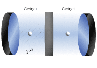
Figure 1: Coupled cavities with a qubit in each and a $\chi^{(2)}$ non-linear medium in the first cavity.

Here, a second order nonlinear process is triggered by adding a $\chi^{(2)}$ medium in the first cavity. Where, a single $\omega_{b}$ photon is converted into two $\omega_{c}$ photons by degenerate SPDC [see Fig. 1]. Now, the Hamiltonian of the system includes an additional term [38, 64] $\hat{H}_{k}$, as,

$$\hat{H}_{k}=i\frac{k}{2}\left[{\left({a_{1}}^{\dagger}\right)}^{2}b-\left({a_{1}}\right)^{2}{b}^{\dagger}\right]+\omega_{b}b^{\dagger}b.$$ (17)

where, $k$ is the non-linear coupling between the $\omega_{c}$ mode and the $\omega_{b}$ mode. The operator $b$ $(b^{\dagger})$ is the annihilation (creation) operator for the bosonic mode. By representing $\omega_{b}$ mode as ‘$\mbox{field}_{b}$’, cavities as ‘$\mbox{field}_{i}$’ and qubits as ‘$\mbox{qubit}_{i}$’, an elementary product state may be written as,

$$\ket{\psi}=\ket{\mbox{qubit}_{1},\,\mbox{field}_{1},\,\mbox{field}_{b},\,\mbox{qubit}_{2},\,\mbox{field}_{2}}$$ (18)

For a maximum of single excitation in $\omega_{b}$ mode, the general state takes the form,

$$\ket{\psi(t)}= \chi(t)\ket{00100}+a(t)\ket{11000}+b(t)\ket{10010}$$

$$+c(t)\ket{10001}+d(t)\ket{01001}+e(t)\ket{01010}$$

$$+f(t)\ket{00011}+g(t)\ket{02000}+h(t)\ket{00002}.$$

Now, the dynamics of the system can be studied by solving the following coupled differential equations, which follows from the Schrödinger equation.

$$i\frac{\partial}{\partial t}\chi(t) =\omega\chi(t)-i\frac{k}{\sqrt{2}}g(t)\,,$$ (20)

$$i\frac{\partial}{\partial t}a(t) =\omega a(t)+\sqrt{2}\lambda g(t)+Jc(t)\,,$$ (21)

$$i\frac{\partial}{\partial t}b(t) =\omega b(t)+\lambda e(t)+\lambda c(t)\,,$$ (22)

$$i\frac{\partial}{\partial t}c(t) =\omega c(t)+\lambda d(t)+\lambda b(t)+Ja(t)\,,$$ (23)

$$i\frac{\partial}{\partial t}d(t) =\omega d(t)+\lambda c(t)+\lambda e(t)+\sqrt{2}Jh(t)+\sqrt{2}Jg(t)\,,$$ (24)

$$i\frac{\partial}{\partial t}e(t) =\omega e(t)+\lambda d(t)+\lambda b(t)+Jf(t)\,,$$ (25)

$$i\frac{\partial}{\partial t}f(t) =\omega f(t)+\sqrt{2}\lambda h(t)+Je(t)\,,$$ (26)

$$i\frac{\partial}{\partial t}g(t) =\omega g(t)+\sqrt{2}\lambda a(t)+\sqrt{2}Jd(t)+i\frac{k}{\sqrt{2}}\chi(t)\,,$$ (27)

$$i\frac{\partial}{\partial t}h(t) =\omega h(t)+\sqrt{2}\lambda f(t)+\sqrt{2}Jd(t)\,.$$ (28)

In the above coupled equations we have taken, $\omega_{b}=2\omega_{c}=2\omega_{a}=2\omega$ and $\lambda_{i}=\lambda$. The Eqs. (20)–(28) can be solved using the Laplace transform method used earlier. Here, for a given set of initial conditions, we solve the differential equations numerically [65].

Case 1. Single excitation in $\omega_{b}$

We start with a single excitation of $\omega_{b}$ mode, $\ket{\psi(0)}=\ket{00100}$, which undergoes degenerate SPDC resulting in two $\omega_{c}$ photons. These photons can interact with the qubits through the coupling $\lambda$, tunnel between the cavities, for non zero values of $J$ and also undergo up conversion to $\omega_{b}$. The population inversion $\braket{\sigma_{z}}$, for qubits ($Q1$ and $Q2$), harmonically oscillates between $-1$ (ground state $\ket{0}$) and zero (superposed state $\left(\ket{0}+\ket{1}\right)/\sqrt{2}$). Behaviour of $\sigma_{z}$ suggest a correlation between the qubits [see Fig. 2]. Here, the overall harmonic behaviour of the qubits does not change as the time passes by.

Case 2. Entangled initial state, $\left(\ket{00100}+\ket{01001}\right)/\sqrt{2}$

To illustrate the dependency of nonlinear coupling, we repeat it for a different initial state and $k$ values. For $\ket{\psi(0)}=\left(\ket{00100}+\ket{01001}\right)/\sqrt{2}$, where the subsystems are entangled, the system does not preserve the identical behaviour as exhibited in the previous case. This means the characteristics of temporal evolution of qubits depends more on the initial state rather than it depends on the coupling factors. For the numerical analysis we have taken $\omega=10\times 2\pi$ GHz, $\lambda=0.1\,\omega$ and $J=0.05\,\lambda$ [see Fig. 2].

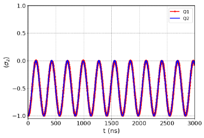
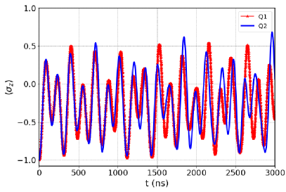
Figure 2: Population inversion, $\braket{\sigma_{z}}$, of qubit 1 (red colour) and qubit 2 (blue colour) for $\omega=10\times 2\pi$ GHz, $\lambda=0.1\,\omega$, $J=0.05\,\lambda$, $k=0.010\,\omega$ and (a) $\ket{\psi(0)}=\ket{00100}$ (b) $\ket{\psi(0)}=\left(\ket{00100}+\ket{01001}\right)/\sqrt{2}$ .

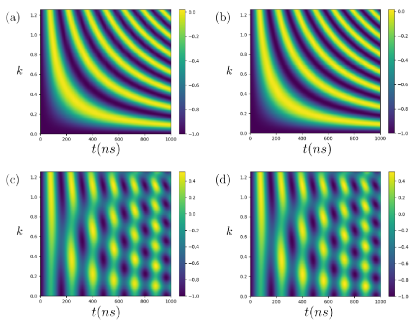
Figure 3: Population inversion for different $k$ values (a) qubit 1 and (b) qubit2 for the initial state $\ket{00100}$. (c) qubit 1 and (d) qubit 2 for the initial state $\left(\ket{00100}+\ket{01001}\right)/\sqrt{2}$, $\Delta=0$.

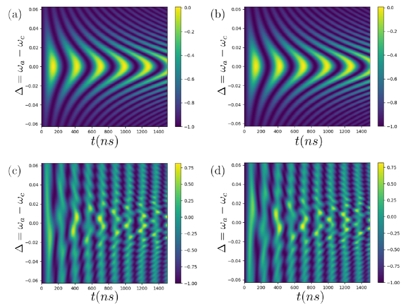
Figure 4: Population inversion for different detuning $\Delta$ (a) qubit 1 and (b) qubit2 for the initial state $\ket{00100}$. (c) qubit 1 and (d) qubit 2 for the initial state $\left(\ket{00100}+\ket{01001}\right)/\sqrt{2}$, $k=0.010\omega$.

Changing the value of $k$ affects the oscillation irrespective of the initial states. Further we spanned $k$ over a range and studied the dynamics. The results are shown in Fig. 3. From the figures, it is evident that various values of coupling factors can bring changes in the dynamics of the system. For the first case, an increase in $k$ increases the oscillation rate. But the amplitude of the system remains unaffected. On the other hand, in the second case, we can see responses in the amplitude of the oscillations and the dynamics does not always carries a simple harmonic behaviour. In the second case, the qubits behaves rather differently, as the time passes by.

The response of the system will depend on the detuning present in the configuration. To confirm this, we extend our studies to off resonant cases. Till now, the cavity mode ($\omega_{c}$) and the atomic transition frequency ($\omega_{a}$) were same. Thus the detuning, $\Delta=\omega_{a}-\omega_{c}$ was zero. Figure 4 shows the sensitivity of the system to detuning. As detuning increases, the amplitude of population inversion is reduced for both cases. Similar to the variation of $k$ in the first case, detuning affects the oscillation rate. Despite the nonlinear process being confined to one cavity, for the special case with $\ket{\psi(0)}=\ket{00100}$, both positive and negative $\Delta$ yields identical results. But the asymmetry in the configuration can be seen in the second case, where we can clearly distinguish between positive and negative detuning as well as qubit 1 and qubit 2. To elaborate further on the temporal characteristics of qubits, we will investigate other measure such as entropy and mutual information in the later section.

In conclusion, various values for coupling constants produce notable differences in the dynamics of the system. Hence, a tunable configuration brings the freedom to tailor the dynamics according to the need. Variation in coupling factor can be introduced by making it time dependent. Time dependent coupling schemes has been addressed in cavity systems before [66]. In the next section we introduce a tunable time dependent nonlinear coupling and investigate the outcome of such a phenomenological model.

4 Time dependent nonlinear coupling

Tunable and enhanced non-linearities have been reported in various composite[67, 68, 59, 60, 61, 62, 63], especially 2D nano materials. This allows us to theoretically propose a tunable harmonic time dependence on the nonlinear coupling factor $k$. For this purpose, we propose a harmonic time dependence as,

$$k(t)\equiv k_{0}\left[1+\sin\left(\Omega t\right)\right],$$ (29)

Here $\Omega$ can vary from zero to infinity, making it as the tunable parameter. When $\Omega=0$ we get the constant coupling as earlier. Table (4), gives the numerical values connecting $t$, $\Omega$ and $k$ in the first cycle. We look at the signature of the time dependence of $k$ over the interval in which the value of $k$ decreases from $10\%$ of the maximum value of $k$ to zero and further increases to $10\%$ of the maximum value of $k$. Previously, as $k$ is increased, we have seen an increase in the oscillatory behaviour of qubits for case 1 and non periodic variation in the inversion amplitude for case 2. By tuning the nonlinear coupling we could surpass this and achieve much stable dynamics for a desired period of time. The choice of when to reduce or increase $k$ depends on $\Omega$. And this gives the freedom to tune and control the system with other coupling factor ($\lambda$ and $J$). From Table (4), as $\Omega$ increases, there is a shift as well as a reduction in the period over which, the value of $k$ decreases from $10\%$ of the maximum value of $k$ to zero and further increases to $10\%$ of the maximum value of $k$. In principle we could independently modulate these two features by adding other harmonic terms.

Numerical values connecting $t$, $\Omega$ and $k$ $\Omega$ Time at $10\%k_{0}$ Time at $k=0$ Time at $10\%k_{0}$ (GHz) (ns) (ns) (ns) 0.000000 – – – 0.002222 1917.7 2120.6 2323.5 0.004444 958.8 1060.3 1161.8 0.006667 639.1 706.8 774.5 0.008889 479.3 530.1 580.9

The population inversion of the qubits, for the initial state $\ket{00100}$ and $\left(\ket{00100}+\ket{01001}\right)/\sqrt{2}$ and $\Omega=0.004444$ GHz are shown in the Figs. 5 and 5.

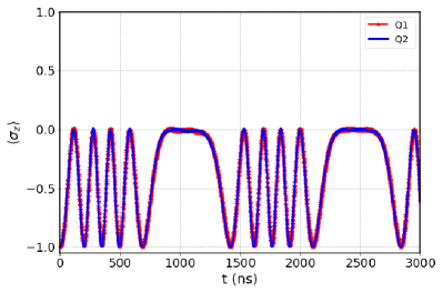
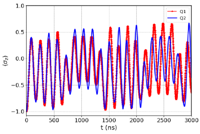
Figure 5: Population inversion $\braket{\sigma_{z}}$, of qubit 1 (red colour) and qubit 2 (blue colour) for $\omega=10\times 2\pi$ GHz, $\lambda=0.1\omega$, $J=0.05\lambda$, $\Omega=0.004444$ GHz and $k_{0}=0.01\omega$. (a) $\ket{\psi(0)}=\ket{00100}$ (b) $\ket{\psi(0)}=\frac{1}{\sqrt{2}}\left(\ket{00100}+\ket{01001}\right)$.

The figures clearly shows a preservation plateaus around the period 950 $\sim$ 1200 $ns$ for both cases [see Table. (4)]. Hence, we can say that this phenomena is independent of the initial state. It is interesting to note that, we could preserve different dynamics [see Fig. 5] during the next similar interval. Thus the preservation is also independent of the state at which the preservation period starts. To better understand this, we repeated the calculation for $\Omega$ ranges from $0$ to $0.01$ GHz. Figure 6 shows the dynamics of qubits 1 and 2 for a range of $\Omega$ and different initial states with $k_{0}=0.01\omega$. With $\ket{\psi(0)}=\ket{00100}$, when $\Omega=0$, we see the inversion as it was without the time dependent coupling. When $\Omega$ increases, value of $k$ also increases. In the previous section, for the same initial conditions, an increase in $k$ resulted in increased oscillatory rate. This is clearly seen in time dependent case as well.

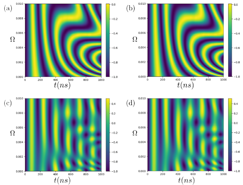
Figure 6: Effect of various time dependent $k$ on population inversion of qubit in cavities. (a) and (b) qubit in the cavities 1 and 2 for the initial state $\ket{00100}$. (c) and (d) qubit in the cavities 1 and 2 for the initial state $\frac{1}{\sqrt{2}}\left(\ket{00100}+\ket{01001}\right)$, $k_{0}=0.010\omega_{c}$, $\Delta=0$.

After reaching the maximum, value of $k$ will start to descend. This must result in the reduction of oscillation rate. In the Fig. 6, we can identify this reduction by the increase in the width of the colour bands. The dynamics gets more interesting when the value of $k$ decreases from $10\%$ of the maximum value of $k$ to zero and further increases to $10\%$ of the maximum value of $k$. We can see preservation plateaus appearing in the figure. The analysis clearly shows that this plateaus appears for the all ranges of $\braket{\sigma_{z}}$. For example, in the Fig. 6 (a), when $\Omega\approx 0.0067$ GHz, a preservation plateau appears for the time interval approximately around 650 ns to 750 ns, with $\braket{\sigma_{z}}\approx-1$. Similarly, when $\Omega\approx 0.006$ GHz, a preservation plateau appears for the time interval approximately around 750 ns to 850 ns, with $\braket{\sigma_{z}}\approx-0.2$. After this preservation period, when $k$ starts to increase, the dynamical behaviour revive and goes on till the next preservation period arrives. These preservation slots can also be seen for $\ket{\psi(0)}=\left(\ket{00100}+\ket{01001}\right)/\sqrt{2}$ ,where, a harmonic oscillatory behaviour is preserved. Such that the population inversion oscillates between, a particular range harmonically [see Figs. 5, 6(c) and 6(d)].

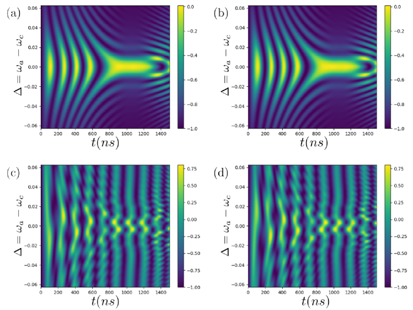
Figure 7: Effect of detuning in time dependent $k$ on population inversion of qubit in cavities. (a) and (b) qubit in the cavities 1 and 2 for the initial state $\ket{00100}$. (c) and (d) qubit in the cavities 1 and 2 for the initial state $\frac{1}{\sqrt{2}}\left(\ket{00100}+\ket{01001}\right)$, $\Omega=0.004444$ GHz and $k_{0}=0.010\omega_{c}$.

The system is further studied for off resonant region, with $\omega_{a}\neq\omega_{c}$. Even in the time dependent coupling scheme, detuning affects the dynamics. Figure 7 shows the results on the new configuration. The figure also highlights the preservation slots for both initial states. As in the time independent case, here we can see identical behaviour for both positive and negative detuning for the special case with initial state as $\ket{00100}$. For the next case, this symmetry is again not seen.

This indicates that, whenever we need to control a certain behaviour, we can do so by controlling the coupling factors. In this particular case, we have seen that, a time dependent nonlinear coupling preserves the dynamics of qubits for a tunable period. To address the characteristics of qubits, we further analyse the system. Using mutual information and von Neumann entropy to quantify the quantumness of system. In the next section, we present an overlook of these measures and calculate the same for our system.

5 Mutual Information and von Neumann entropy

A probabilistic theory cannot yield deterministic results due to the lack of information. Hence, one has to account for this lack of information and deduce the physics. Works by Shannon [69] and Neumann [70] clearly formulate this lack of information as the entropy of the system. It can account, not only the classical probabilities but also the quantumness present in the configuration. Here we use mutual information (mutual entropy) and von Neumann entropy.

Mutual information (MI) quantifies the amount of information shared between two systems [71], and is defined as:

$$I(X:Y)=H(X)+H(Y)-H(X,Y)\,.$$ (30)

Where $H(X)$ and $H(Y)$ is the Shannon entropy and $H(X,Y)$ is the joint Shannon entropy. Classically, the above equation corresponds to the relative entropy with,

$$H(X,Y)\geq H(X)\,\mbox{or}\,H(Y).$$ (31)

The quantum analogue of Shannon entropy is the von Neumann entropy [72] ($S$), from which the quantum analogue for mutual information takes the form,

$$I(m:n)=S\left(\rho_{m}\right)+S\left(\rho_{n}\right)-S\left(\rho_{mn}\right),$$ (32)

where $\rho$ is the density matrix and $m,n$ are the indices of the subsystems (sub Hilbert-spaces). Here, $\rho_{mn}$ and $\rho_{m}$ corresponds to the composite system and subsystem respectively. One can find $\rho_{m}$ by taking the partial trace of $\rho_{mn}$ over $n$. Now the inequality becomes,

$$S\left(\rho_{mn}\right)\geq S\left(\rho_{n}\right)$$ (33)

The violation of the above inequality [Eq. (33)] indicates the presence of entanglement in the system. A general expression for entropy in quantum mechanics is given as,

$$S_{\alpha}\left(\rho_{m}\right)=\left(1-\alpha\right)^{-1}\log\mbox{Tr}\left(\rho_{m}\right)^{\alpha},$$ (34)

This is known as the $\alpha$-entropy or the Rényi $\alpha$-entropy. Equation (34) reduces to von Neumann entropy for the limit $\alpha\to 1$ as,

$$S\left(\rho_{m}\right)=-\mbox{Tr}\left(\rho_{m}\log_{2}\rho_{m}\right).$$ (35)

Expressions in Eqs. (32) and (35) are used for our analysis. We numerically compute $\rho$ as a function of time and then calculate the entropies to better understand the quantum states of the system.

5.1 Von Neumann Entropy

For von Neumann entropy, first we numerically compute $\ket{\psi(t)}$ using the initial conditions and the time dependent Hamiltonian with the time dependent coupling in Eq. (29), and thus obtain $\rho(t)$. Since we are interested in the dynamics of qubits, we trace over the rest of the subsystems and found $\rho_{q1}$ and $\rho_{q2}$. Finally, using the Eq. (32), we computed the von Neumann entropy of the qubits, with initial conditions $\ket{\psi(0)}=\ket{00100}$ and $\ket{\psi(0)}=\left(\ket{00100}+\ket{01001}\right)/\sqrt{2}$.

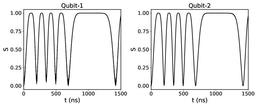
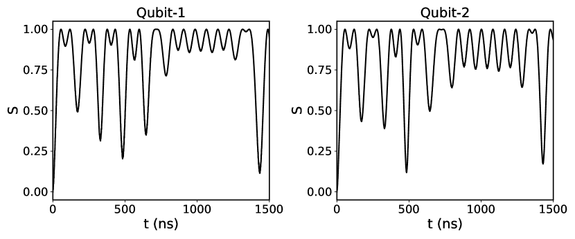
Figure 8: Von Neumann entropy (a) $\ket{\psi(0)}=\ket{00100}$ and (b) $\ket{\psi(0)}=\frac{1}{\sqrt{2}}\left(\ket{00100}+\ket{01001}\right)$.

The results of both initial states are shown in Figs. 8 and 8. For the first case, with $\ket{\psi(0)}=\ket{00100}$, the qubits reaches the maximum possible value of $S$ and tends to remain in that state during the preservation period. Since the states are not mixed, this maximum value of von Neumann entropy corresponds to a maximally entangled state ($S=1$). For a different value of $\Omega$, one may preserve a non maximal entanglement ($1>S>0$) or a pure state ($S=0$).

For the second case with $\ket{\psi(0)}=\left(\ket{00100}+\ket{01001}\right)/\sqrt{2}$, the qubits tends to preserve the dynamics during the preservation slot. Before the preservation slot, the von Neumann entropy of the qubits oscillates with larger amplitude difference. But during the time, the oscillation amplitude remains rather consistent. This confirms the preservation of the dynamics of the qubits. Further we did the same analysis on other subsystems present in the configuration and the results are show in Fig.9.

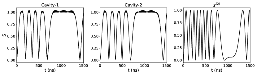
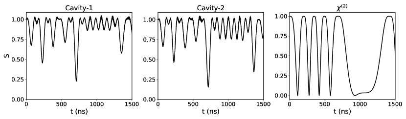
Figure 9: Von Neumann entropy (a) $\ket{\psi(0)}=\ket{00100}$ and (b) $\ket{\psi(0)}=\frac{1}{\sqrt{2}}\left(\ket{00100}+\ket{01001}\right)$.

Here, the small fluctuations in the preservation plateau is due to other coupling factors, such as photon hopping in the system. It has to be note that, the von Neumann entropy of the cavity modes and $\chi^{(2)}$ mode started from a non zero value in the second case [see Fig. 9]. This clearly indicates the initial entanglement between the subsystems. But they are not the maximum, this is because of the sharing of entanglement between the cavity modes. Even though we could infer the entanglement of a subsystem, von Neumann entropy cannot reveal about which subsystem it is entangled to. To address this one must calculate a measure, which incorporate two subsystems at once. Here we use mutual information, defined in Eq. (32), as our measure for the same.

5.2 Mutual Information

Earlier, we found that there is an entanglement present between our subsystems. In this section, we compute the mutual information between each pairs of subsystems to understand the distribution of information. Mutual information is measured between two subsystem, since we have five subsystems, we need to compute the partially reduced density matrices, such that each pairs are accounted. For example, to study mutual information between qubit 1 and qubit 2, we trace out the cavities and other bosonic modes from the complete density matrix, ($\rho$) such that we end up with a partially reduced density matrix ($\rho_{q1q2}$). We also find the completely reduced density matrix $\rho_{q1}$ and $\rho_{q2}$. Now we calculate the von Neumann entropies and compute mutual information as,

$$I(q1:q2)=S\left(\rho_{q1}\right)+S\left(\rho_{q2}\right)-S\left(\rho_{q1q2}\right),$$ (36)

For this, we choose our initial state and compute the density matrices as a function of time. Further, the reduced ($\rho_{m}$) and partially reduced ($\rho_{mn}$) density matrices were computed, after which we proceed to compute mutual information as discussed above. The procedure is repeated for all such pairs in the configuration. Here, the initial states considered are $\ket{\psi(0)}=\ket{00100}$ and $\ket{\psi(0)}=\left(\ket{00100}+\ket{01001}\right)/\sqrt{2}$ with $\Omega=0.004444$ GHz. For consistency, the coupling constants retains the previously assigned values.

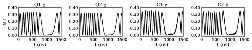
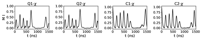
Figure 10: Mutual information for (a) $\ket{\psi(0)}=\ket{00100}$ and (b) $\ket{\psi(0)}=\frac{1}{\sqrt{2}}\left(\ket{00100}+\ket{01001}\right)$.

Figures 10 and 10 shows the mutual information between the qubits and cavities with the $\chi^{(2)}$ bosonic mode for different initial conditions. As expected, the $\chi^{(2)}$ bosonic mode appears to share less information during the preservation time, since its coupling to the system has been reduced. We can see our initial entanglement between the cavity modes and the $\chi^{(2)}$ bosonic mode, in the second case as a non zero mutual information. Further, in Fig. 11, we can also see an entanglement between the cavity 1 and 2. Thus, the entanglement we inferred from the von Neumann entropy is not bipartite.

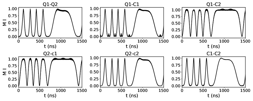
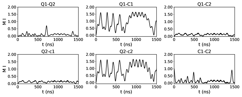
Figure 11: Mutual information for (a) $\ket{\psi(0)}=\ket{00100}$ and (b) $\ket{\psi(0)}=\frac{1}{\sqrt{2}}\left(\ket{00100}+\ket{01001}\right)$.

For cases 1 and 2, the qubits has a non zero mutual information between all other subsystems making a multipartite entanglement. And the time dependent coupling makes it possible to preserve it during the preservation slots. An ideal situation where the entanglement is completely preserved is when there is no interaction. Thus it is practically challenging to preserve it. Here, by using a time dependent non-linear coupling, we have preserved the entanglement produced in the configuration.

6 Conclusion

In this work, we have studied two coupled cavity with a single qubit in each and a second order nonlinear process in one of the cavity. The configuration for different values of nonlinear coupling and off resonant regimes are investigated and found that the system is highly sensitive to detuning. Further introduction of a harmonic time dependence on the nonlinear coupling has been utilized for the preservation of dynamics of the qubits. It is found that, a harmonic coupling with a control parameter, $\Omega$, can preserve the dynamics of the qubits for an interval irrespective of the choice of initial state. We further calculated the von Neumann entropy and mutual information to account for the entanglement present between the subsystem. From which it is found that, the preservation plateau also preserves the entanglement produced in the configuration.

References

- [1] Benjamin Schumacher. Quantum coding. Phys. Rev. A, 51:2738–2747, Apr 1995.
- [2] E. T. Jaynes and F. W. Cummings. Comparison of quantum and semiclassical radiation theories with application to the beam maser. Proceedings of the IEEE, 51(1):89–109, Jan 1963.
- [3] P. Góra and C. Jedrzejek. Nonlinear jaynes-cummings model. Phys. Rev. A, 45:6816–6828, May 1992.
- [4] J. Črnugelj, M. Martinis, and V. Mikuta-Martinis. Properties of a deformed jaynes-cummings model. Phys. Rev. A, 50:1785–1791, Aug 1994.
- [5] R. H. Dicke. Coherence in spontaneous radiation processes. Phys. Rev., 93:99–110, Jan 1954.
- [6] T. D. Ladd, F. Jelezko, R. Laflamme, Y. Nakamura, C. Monroe, and J. L. O’Brien. Quantum computers. Nature, 464:45 EP –, Mar 2010. Review Article.
- [7] Giuliano Benenti, Giulio Casati, and Giuliano Strini. Principles of Quantum Computation and Information. WORLD SCIENTIFIC, 2004.
- [8] Artur Ekert and Richard Jozsa. Quantum computation and shor’s factoring algorithm. Rev. Mod. Phys., 68:733–753, Jul 1996.
- [9] I. M. Georgescu, S. Ashhab, and Franco Nori. Quantum simulation. Rev. Mod. Phys., 86:153–185, Mar 2014.
- [10] R. Blatt and C. F. Roos. Quantum simulations with trapped ions. Nature Physics, 8:277 EP –, Apr 2012. Review Article.
- [11] Daniel E. Browne and Terry Rudolph. Resource-efficient linear optical quantum computation. Phys. Rev. Lett., 95:010501, Jun 2005.
- [12] H. Jeong and M. S. Kim. Efficient quantum computation using coherent states. Phys. Rev. A, 65:042305, Mar 2002.
- [13] Sean D. Barrett and Pieter Kok. Efficient high-fidelity quantum computation using matter qubits and linear optics. Phys. Rev. A, 71:060310, Jun 2005.
- [14] E. Knill, R. Laflamme, and G. J. Milburn. A scheme for efficient quantum computation with linear optics. Nature, 409:46 EP –, Jan 2001. Article.
- [15] T. E. Northup and R. Blatt. Quantum information transfer using photons. Nature Photonics, 8:356 EP –, Apr 2014. Review Article.
- [16] Dimitris G. Angelakis and Sougato Bose. Generation and verification of high-dimensional entanglement from coupled-cavity arrays. J. Opt. Soc. Am. B, 24(2):266–269, Feb 2007.
- [17] Jaeyoon Cho, Dimitris G. Angelakis, and Sougato Bose. Heralded generation of entanglement with coupled cavities. Phys. Rev. A, 78:022323, Aug 2008.
- [18] Tong Liu, Qi-Ping Su, Shao-Jie Xiong, Jin-Ming Liu, Chui-Ping Yang, and Franco Nori. Generation of a macroscopic entangled coherent state using quantum memories in circuit qed. Scientific Reports, 6:32004 EP –, Aug 2016. Article.
- [19] J. Robert Johansson, Neill Lambert, Imran Mahboob, Hiroshi Yamaguchi, and Franco Nori. Entangled-state generation and bell inequality violations in nanomechanical resonators. Phys. Rev. B, 90:174307, Nov 2014.
- [20] Bastian Hacker, Stephan Welte, Severin Daiss, Armin Shaukat, Stephan Ritter, Lin Li, and Gerhard Rempe. Deterministic creation of entangled atom-light schrödinger-cat states. Nature Photonics, 13(2):110–115, 2019.
- [21] Zhong-Xiao Man, Yun-Jie Xia, and Rosario Lo Franco. Cavity-based architecture to preserve quantum coherence and entanglement. Scientific Reports, 5:13843 EP –, Sep 2015. Article.
- [22] Jiong Cheng, Wen-Zhao Zhang, Ling Zhou, and Weiping Zhang. Preservation macroscopic entanglement of optomechanical systems in non-markovian environment. Scientific Reports, 6:23678 EP –, Apr 2016. Article.
- [23] Ali Mortezapour and Rosario Lo Franco. Protecting quantum resources via frequency modulation of qubits in leaky cavities. Scientific Reports, 8(1):14304, 2018.
- [24] Adeline Orieux, Antonio D’Arrigo, Giacomo Ferranti, Rosario Lo Franco, Giuliano Benenti, Elisabetta Paladino, Giuseppe Falci, Fabio Sciarrino, and Paolo Mataloni. Experimental on-demand recovery of entanglement by local operations within non-markovian dynamics. Scientific Reports, 5:8575 EP –, Feb 2015. Article.
- [25] Jin-Shi Xu, Kai Sun, Chuan-Feng Li, Xiao-Ye Xu, Guang-Can Guo, Erika Andersson, Rosario Lo Franco, and Giuseppe Compagno. Experimental recovery of quantum correlations in absence of system-environment back-action. Nature Communications, 4:2851 EP –, Nov 2013. Article.
- [26] Wolfgang Pfaff, Christopher J. Axline, Luke D. Burkhart, Uri Vool, Philip Reinhold, Luigi Frunzio, Liang Jiang, Michel H. Devoret, and Robert J. Schoelkopf. Controlled release of multiphoton quantum states from a microwave cavity memory. Nature Physics, 13:882 EP –, Jun 2017. Article.
- [27] Peng Xu, Xu-Chen Yang, Feng Mei, and Zheng-Yuan Xue. Controllable high-fidelity quantum state transfer and entanglement generation in circuit qed. Scientific Reports, 6:18695 EP –, Jan 2016. Article.
- [28] Jin-Lei Wu, Xin Ji, and Shou Zhang. Fast adiabatic quantum state transfer and entanglement generation between two atoms via dressed states. Scientific Reports, 7:46255 EP –, Apr 2017. Article.
- [29] T. M. Manosh, Muhammed Ashefas, and Ramesh Babu Thayyullathil. Effects of kerr medium in coupled cavities on quantum state transfer. Journal of Nonlinear Optical Physics & Materials, 27(03):1850035, 2018.
- [30] J. C. Retamal and C. Saavedra. Enhanced transient squeezing in a kicked jaynes-cummings model. Phys. Rev. A, 50:1867–1870, Aug 1994.
- [31] J. R. Kukliński and J. L. Madajczyk. Strong squeezing in the jaynes-cummings model. Phys. Rev. A, 37:3175–3178, Apr 1988.
- [32] Adam Stokes and Ahsan Nazir. Gauge ambiguities imply jaynes-cummings physics remains valid in ultrastrong coupling qed. Nature Communications, 10(1):499, 2019.
- [33] Lucia Caspani, Chunle Xiong, Benjamin J. Eggleton, Daniele Bajoni, Marco Liscidini, Matteo Galli, Roberto Morandotti, and David J. Moss. Integrated sources of photon quantum states based on nonlinear optics. Light: Science &Amp; Applications, 6:e17100 EP –, Nov 2017. Review.
- [34] Ling-An Wu, H. J. Kimble, J. L. Hall, and Huifa Wu. Generation of squeezed states by parametric down conversion. Phys. Rev. Lett., 57:2520–2523, Nov 1986.
- [35] Paul G. Kwiat, Klaus Mattle, Harald Weinfurter, Anton Zeilinger, Alexander V. Sergienko, and Yanhua Shih. New high-intensity source of polarization-entangled photon pairs. Phys. Rev. Lett., 75:4337–4341, Dec 1995.
- [36] M T Manzoni, I Silveiro, F J García de Abajo, and D E Chang. Second-order quantum nonlinear optical processes in single graphene nanostructures and arrays. New Journal of Physics, 17(8):083031, aug 2015.
- [37] Hatef Dinparasti Saleh, Stefano Vezzoli, Lucia Caspani, Artur Branny, Santosh Kumar, Brian D. Gerardot, and Daniele Faccio. Towards spontaneous parametric down conversion from monolayer mos2. Scientific Reports, 8(1):3862, 2018.
- [38] P.D. Drummond, K.J. McNeil, and D.F. Walls. Non-equilibrium transitions in sub/second harmonic generation. Optica Acta: International Journal of Optics, 27(3):321–335, 1980.
- [39] Bartosz Regula and Gerardo Adesso. Entanglement quantification made easy: Polynomial measures invariant under convex decomposition. Phys. Rev. Lett., 116:070504, Feb 2016.
- [40] W. Vogel and J. Sperling. Unified quantification of nonclassicality and entanglement. Phys. Rev. A, 89:052302, May 2014.
- [41] Alexander A. Klyachko, Barı ş Öztop, and Alexander S. Shumovsky. Quantification of entanglement via uncertainties. Phys. Rev. A, 75:032315, Mar 2007.
- [42] F. Shahandeh, J. Sperling, and W. Vogel. Structural quantification of entanglement. Phys. Rev. Lett., 113:260502, Dec 2014.
- [43] Yaakov S. Weinstein. Tripartite entanglement witnesses and entanglement sudden death. Phys. Rev. A, 79:012318, Jan 2009.
- [44] Bartosz Regula and Gerardo Adesso. Geometric approach to entanglement quantification with polynomial measures. Phys. Rev. A, 94:022324, Aug 2016.
- [45] Yu Luo, Fu-Gang Zhang, and Yongming Li. Entanglement distribution in multi-particle systems in terms of unified entropy. Scientific Reports, 7(1):1122, 2017.
- [46] A. Mari, A. Farace, N. Didier, V. Giovannetti, and R. Fazio. Measures of quantum synchronization in continuous variable systems. Phys. Rev. Lett., 111:103605, Sep 2013.
- [47] Minghui Xu, D. A. Tieri, E. C. Fine, James K. Thompson, and M. J. Holland. Synchronization of two ensembles of atoms. Phys. Rev. Lett., 113:154101, Oct 2014.
- [48] O. V. Zhirov and D. L. Shepelyansky. Synchronization and bistability of a qubit coupled to a driven dissipative oscillator. Phys. Rev. Lett., 100:014101, Jan 2008.
- [49] V. Ameri, M. Eghbali-Arani, A. Mari, A. Farace, F. Kheirandish, V. Giovannetti, and R. Fazio. Mutual information as an order parameter for quantum synchronization. Phys. Rev. A, 91:012301, Jan 2015.
- [50] Gonzalo Manzano, Fernando Galve, Gian Luca Giorgi, Emilio Hernández-García, and Roberta Zambrini. Synchronization, quantum correlations and entanglement in oscillator networks. Scientific Reports, 3:1439 EP –, Mar 2013. Article.
- [51] Akshay Seshadri, Vaibhav Madhok, and Arul Lakshminarayan. Tripartite mutual information, entanglement, and scrambling in permutation symmetric systems with an application to quantum chaos. Phys. Rev. E, 98:052205, Nov 2018.
- [52] Niels Lörch, Ehud Amitai, Andreas Nunnenkamp, and Christoph Bruder. Genuine quantum signatures in synchronization of anharmonic self-oscillators. Phys. Rev. Lett., 117:073601, Aug 2016.
- [53] Alexandre Roulet and Christoph Bruder. Quantum synchronization and entanglement generation. Phys. Rev. Lett., 121:063601, Aug 2018.
- [54] Tony E. Lee, Ching-Kit Chan, and Shenshen Wang. Entanglement tongue and quantum synchronization of disordered oscillators. Phys. Rev. E, 89:022913, Feb 2014.
- [55] Michael R. Hush, Weibin Li, Sam Genway, Igor Lesanovsky, and Andrew D. Armour. Spin correlations as a probe of quantum synchronization in trapped-ion phonon lasers. Phys. Rev. A, 91:061401, Jun 2015.
- [56] Niels Lörch, Simon E. Nigg, Andreas Nunnenkamp, Rakesh P. Tiwari, and Christoph Bruder. Quantum synchronization blockade: Energy quantization hinders synchronization of identical oscillators. Phys. Rev. Lett., 118:243602, Jun 2017.
- [57] Simon E. Nigg. Observing quantum synchronization blockade in circuit quantum electrodynamics. Phys. Rev. A, 97:013811, Jan 2018.
- [58] F. K. Nohama and J. A. Roversi. Quantum state transfer between atoms located in coupled optical cavities. Journal of Modern Optics, 54(8):1139–1149, 2007.
- [59] J. W. You and N. C. Panoiu. Tunable enhancement of second-harmonic generation in dual graphene optical gratings. In 2017 11th International Congress on Engineered Materials Platforms for Novel Wave Phenomena (Metamaterials), pages 382–384, Aug 2017.
- [60] Jian Wei You, Jie You, Martin Weismann, and Nicolae C. Panoiu. Double-resonant enhancement of third-harmonic generation in graphene nanostructures. Philosophical Transactions of the Royal Society A: Mathematical, Physical and Engineering Sciences, 375(2090):20160313, 2017.
- [61] Daria A. Smirnova, Andrey E. Miroshnichenko, Yuri S. Kivshar, and Alexander B. Khanikaev. Tunable nonlinear graphene metasurfaces. Phys. Rev. B, 92:161406, Oct 2015.
- [62] Joel D. Cox, Iván Silveiro, and F. Javier García de Abajo. Quantum effects in the nonlinear response of graphene plasmons. ACS Nano, 10(2):1995–2003, 2016. PMID: 26718484.
- [63] Joel D. Cox and F. Javier García de Abajo. Plasmon-enhanced nonlinear wave mixing in nanostructured graphene. ACS Photonics, 2(2):306–312, 2015.
- [64] Vlatko Vedral. Modern foundations of quantum optics. Imperial College Press, 2006.
- [65] J.R. Johansson, P.D. Nation, and Franco Nori. Qutip: An open-source python framework for the dynamics of open quantum systems. Computer Physics Communications, 183(8):1760 – 1772, 2012.
- [66] Amitabh Joshi and S.V. Lawande. Generalized jaynes-cummings models with a time dependent atom-field coupling. Phys. Rev. A, 48:2276–2284, Sep 1993.
- [67] Sanfeng Wu, Li Mao, Aaron M. Jones, Wang Yao, Chuanwei Zhang, and Xiaodong Xu. Quantum-enhanced tunable second-order optical nonlinearity in bilayer graphene. Nano Letters, 12(4):2032–2036, 2012. PMID: 22369519.
- [68] Hung-Hsi Lin, Felipe Vallini, Mu-Han Yang, Rajat Sharma, Matthew W. Puckett, Sergio Montoya, Christian D. Wurm, Eric E. Fullerton, and Yeshaiahu Fainman. Electronic metamaterials with tunable second-order optical nonlinearities. Scientific Reports, 7(1):9983, 2017.
- [69] C. E. Shannon. A mathematical theory of communication. Bell System Technical Journal, 27(3):379–423, 1948.
- [70] John von Neumann. Mathematical foundations of quantum mechanics. 1955.
- [71] E. Boukobza and D. J. Tannor. Entropy exchange and entanglement in the jaynes-cummings model. Phys. Rev. A, 71:063821, Jun 2005.
- [72] Ryszard Horodecki, Paweł Horodecki, Michał Horodecki, and Karol Horodecki. Quantum entanglement. Rev. Mod. Phys., 81:865–942, Jun 2009.