Exact solution for progressive gravity waves on the surface of a deep fluid

Abstract

Gerstner or trochoidal wave is the only known exact solution of the Euler equations for periodic surface gravity waves on deep water. In this Letter we utilize Zakharov’s variational formulation of weakly nonlinear surface waves and, without truncating the Hamiltonian in its slope expansion, derive the equations of motion for unidirectional gravity waves propagating in a two-dimensional flow. We obtain an exact solution of the evolution equations in terms of the Lambert $W$-function. The associated flow field is irrotational. The maximum wave height occurs for a wave steepness of 0.2034 which compares to 0.3183 for the trochoidal wave and 0.1412 for the Stokes wave. Like in the case of Gerstner’s solution, the limiting wave of a new type has a cusp of zero angle at its crest.

An exact solution for progressive gravity waves on the surface of a deep fluid

Background.—The water waves problem even in the completely idealized setting of a perfect fluid is notoriously difficult from a mathematical point of view. This is one of the reasons we have very few explicit solutions to the fully nonlinear free-surface hydrodynamics equations despite extensive research over hundreds of years. The first exact solution was provided by Gerstner Gerstner in 1802 for pure gravity waves of finite height propagating on the surface of an inviscid and incompressible fluid of infinite depth. The practical importance of trochoidal waves became apparent when in the 1860s Rankine and Froude independently rediscovered them in connection with the ship-rolling problem Rankine . The fact that these waves are rotational and cannot be generated from the fluid at rest was seen as somewhat unsatisfactory. Moreover, since the fluid particles move on a closed circular orbit, Gerstner’s solution does not predict the observed mass transport in the direction of wave propagation Wiegel .

In 1847 Stokes presented an approximate theory for irrotational waves and showed that for deep water the wave profile coincides with a trochoid to the third order, but not to the fourth Stokes . He also conjectured the existence of the wave of greatest height distinguished by a sharp edge and argued that the enclosing angle must be $120^{\circ}$. The mere existence of such waves was rigorously verified only forty years ago Toland , clearly illustrating the inherently complicated structure of the underlying nonlinear equations. The existence of extreme waves that are, as hypothesized by Stokes, strictly convex between successive crests was established very recently, but in spite of some numerical evidence supporting the convexity of all waves of extreme form their uniqueness remains an open problem Plotnikov .

Apart from Crapper’s exact solution for pure capillary waves Crapper found in 1957 and some explicit Gerstner-type solutions for equatorially trapped waves discovered lately Constantin , the field of exact solutions for water wave equations has not experienced significant advancement since the last century. In this Letter, we present an exact solution for planar periodic waves of finite amplitude moving uniformly and without change of form on a fluid of unlimited depth when only gravity acts as a restoring force. Following Zakharov Zakharov , we use the power of Hamiltonian formalism to write an asymptotic expansion of the equations of motion for a pair of canonically conjugate variables – the surface elevation and the velocity potential evaluated on the free surface. The expansion coefficients simplify remarkably for two-dimensional waves propagating in the same direction and the infinite series can be summed in a closed form if the wave steepness is small. From the stationary periodic solution of the resulting nonlinear equations, an exact irrotational solution to the full system of hydrodynamic equations with a free surface is then recovered. The solutions are provided in Eulerian coordinates fn1 .

Exact solutions play an important role not just because all the properties of the motion can be conveniently expressed and analyzed without any approximation, but also because they can provide a key insight into the nature of more complex and physically more realistic flows, say, in which waves propagate under the combined influence of gravity and surface tension.

Let us finish this introduction with a note that two-dimensional flows are not of purely theoretical interest. Their fundamental importance stems from the observation that in many situations the motion of water waves can be treated as quasi-two-dimensional. For example, waves generated in the open ocean while coming ashore often appear as a wave-train of very long nearly parallel crests Johnson and due to this symmetry can be more or less accurately studied and simulated by various two-dimensional models (see, e.g., Chalikov ).

Theoretical formulation.—The potential flow $\phi(x,y,t)$ of an ideal incompressible fluid in the region $\Omega(t)=\left\{(x,y)\in\mathbb{R}^{2}\colon-\infty<y\leq\xi(x,t)\right\}$ bounded by the free surface $\Gamma(t)=\left\{y=\xi(x,t)\right\}$ satisfies the following set of equations:

$$\xi_{t}+\xi_{x}\phi_{x}-\phi_{y}=0, \mbox{ on }\Gamma(t)$$ (1a)

$$\phi_{t}+\frac{1}{2}\left(\phi_{x}^{2}+\phi_{y}^{2}\right)+g\xi=0, \mbox{ on }\Gamma(t)$$ (1b)

$$\phi_{xx}+\phi_{yy}=0, \mbox{ in }\Omega(t)$$ (1c)

$$\phi_{y}\to 0, \mbox{ as }y\to-\infty$$ (1d)

where $g$ is the constant gravitational acceleration in the negative $y$ direction and subscripts denote partial derivatives. The effects of surface tension are neglected and the pressure at the free surface is taken to be zero. Once $\xi(x,t)$ and $\phi(x,y,t)$ are found, the velocity field and the pressure within the fluid domain follow from

$${\bf v}(x,y,t)=\nabla\phi,$$

$$p(x,y,t)=-\rho\left(gy+\phi_{t}+\frac{|{\bf v}|^{2}}{2}\right)$$

where $\rho$ is the fluid density. Since $\phi$ is harmonic in $\Omega(t)$, it is uniquely determined by its trace on the free boundary, $\psi(x,t)=\left.\phi\right|_{y=\xi(x,t)}$, and (1d). Zakharov ingeniously realized that equations (1a)-(1b) describing the wave motion can be put in the form of Hamilton’s canonical equations

$$\rho\frac{\partial\xi}{\partial t}=\frac{\delta H}{\delta\psi},\ \ \rho\frac{\partial\psi}{\partial t}=-\frac{\delta H}{\delta\xi}$$ (2)

with the Hamiltonian given as the sum of the potential energy measured with respect to the undisturbed fluid level $y=0$ and the kinetic energy Zakharov :

$$H=\frac{\rho}{2}\int_{-\infty}^{\infty}dx\left(g\xi^{2}+\int_{-\infty}^{\xi}|{\bf v}|^{2}dy\right).$$ (3)

The Laplace equation (1c) and the decay condition at infinity (1d) represent the constraints on the dynamical system whose total energy $H$ is a constant of motion.

The major difficulty in applying the Hamiltonian formalism for water waves lies in expressing the kinetic energy in terms of free surface variables, $\xi$ and $\psi$, alone. When the wave steepness is small, $|\xi_{x}|\ll 1$, one can write the expansion of the Hamiltonian in a power series in the amplitudes of the waves. Let $\hat{\xi}_{k}=\hat{\xi}_{-k}^{*}$ and $\hat{\psi}_{k}=\hat{\psi}_{-k}^{*}$ denote the Fourier components of $\xi$ and $\psi$, then upon solving the boundary-value problem for Laplace’s equation the Hamiltonian (3) reads

$$H=\frac{1}{2}\int|k|\hat{\psi}_{0}^{*}\hat{\psi}_{0}+g\hat{\xi}_{0}^{*}\hat{\xi}_{0}dk+$$

$$+\sum_{n=1}^{\infty}\int E_{0,1,2,\dots,n+1}^{(n+2)}\hat{\psi}_{0}\hat{\psi}_{1}\prod_{i=2}^{n+1}\hat{\xi}_{i}\delta\left(\sum_{i=0}^{n+1}k_{i}\right)\prod_{j=0}^{n+1}dk_{j}.$$ (4)

where we set $\rho=1$ fn2 . Computing the expansion kernels $E_{0,1,2,\dots,n+1}^{(n+2)}$ relies on a series reversion associated with expressing the velocity potential in terms of its value at the free surface Krasitskii . These kernels can be obtained in principle to all orders, however, the iteration process quickly becomes cumbersome. A fully explicit recursion relation for computing $E_{0,1,2,\dots,n+1}^{(n+2)}$ without a laborious series reversion has been proposed recently in Ussemb for an arbitrary depth and arbitrary space dimension.

The Fourier transform is a canonical transformation, and hence the evolution equations (2) preserve their Hamiltonian form in the canonically conjugate variables $\hat{\xi}_{k}$ and $\hat{\psi}_{k}$:

$$\frac{\partial\hat{\xi}_{k}}{\partial t}=\frac{\delta H}{\delta\hat{\psi}_{k}^{*}}=|k|\hat{\psi}_{k}+2\sum_{n=1}^{\infty}\int E_{-0,1,2,\dots,n+1}^{(n+2)}\hat{\psi}_{1}\prod_{i=2}^{n+1}\hat{\xi}_{i}\delta\left(k-\sum_{i=1}^{n+1}k_{i}\right)dk_{12\dots n+1},$$ (5a)

$$\frac{\partial\hat{\psi}_{k}}{\partial t}=-\frac{\delta H}{\delta\hat{\xi}_{k}^{*}}=-g\hat{\xi}_{k}-\sum_{n=1}^{\infty}\int nE_{1,2,\dots,n+1,-0}^{(n+2)}\hat{\psi}_{1}\hat{\psi}_{2}\prod_{i=3}^{n+1}\hat{\xi}_{i}\delta\left(k-\sum_{i=1}^{n+1}k_{i}\right)dk_{12\dots n+1}$$ (5b)

where (Exact solution for progressive gravity waves on the surface of a deep fluid) was used to compute the variational derivative. The expansion kernels posses a remarkable property revealed by the recursion relation: for any fixed $n\in\mathbb{N}$, it holds that

$$E_{-\sum_{i=1}^{n+1}k_{i},k_{1},k_{2},\dots,k_{n+1}}^{(n+2)}=0$$ (6)

if all wavenumbers have the same sign Ussemb and

$$E_{k_{1},k_{2},\dots,k_{n+1},-\sum_{i=1}^{n+1}k_{i}}^{(n+2)}=-\frac{\sigma^{n+1}}{n(2\pi)^{n/2}}\prod_{i=1}^{n+1}k_{i}$$ (7)

with $\sigma=-1$ ($\sigma=+1$) if all wavenumbers are positive (resp. negative). Hence, by considering waves traveling in one direction we can drastically simplify the equations of motion. Indeed, taking the inverse Fourier transform of (5) and using (6)-(7) we obtain

$$\xi_{t}^{\pm}\pm i\psi_{x}^{\pm}=0$$ (8a)

$$\psi_{t}^{\pm}+g\xi^{\pm}=\frac{\left(i\psi_{x}^{\pm}\right)^{2}}{1\mp i\xi_{x}^{\pm}}$$ (8b)

where $f^{\pm}=P^{\pm}f$, $P^{\pm}=\frac{1}{2}\left(I\pm i\mathbb{H}\right)$ are orthogonal self-adjoint projections onto positive and negative wavenumber components, $\mathbb{H}$ is the Hilbert transform fn3 . In summary, the small-amplitude assumption, $|\xi_{x}|\ll 1$, in conjunction with the unidirectionality of wave propagation for which relations (6)-(7) are valid in one dimension allows us to write apparently intangible equations (5) containing infinite sums in a concise form given in (8).

A few remarks are in order. First, making a crude approximation $\left(1\mp i\xi_{x}^{\pm}\right)^{-1}=1+{\mathcal{O}}\left(\xi_{x}^{\pm}\right)$ in (8b) and letting $g=0$ reduces the system (8) to the equations (17)-(18) derived in Kuznetsov to study the formation of singularities on the free surface of an ideal fluid in the absence of gravitational force. Second, differentiating (8a) with respect to time and (8b) with respect to space yields the conservation form

$$\left(\xi_{t}^{\pm}\right)_{t}\pm\left(\frac{i\left(\xi_{t}^{\pm}\right)^{2}}{1\mp i\xi_{x}^{\pm}}-ig\xi^{\pm}\right)_{x}=0$$

which uncouples the free surface elevation from $\psi^{\pm}$. Last, using (8a) it is possible to rewrite (8b) as

$$\psi_{t}+g\xi+\frac{1}{2}\psi_{x}^{2}-\frac{1}{2}\frac{\left(\xi_{t}+\xi_{x}\psi_{x}\right)^{2}}{1+\xi_{x}^{2}}=0$$

and (8a) itself as a non-local equation

$$\int_{-\infty}^{\infty}dxe^{-ikx+|k|\xi}\left(i\xi_{t}-\mbox{sgn}(k)\psi_{x}\right)=0$$

valid for every value of $k\in\mathbb{R}$. Thus we can recover from (8) the non-local formulation of Euler’s equations due to Ablowitz, Fokas and Musslimani (c.f. AFM , p. 326). The AFM formulation is particularly useful for deriving various asymptotic approximations including the nonlinear Schrödinger equation describing the envelopes of waves in deep water.

General solution.—Next we attempt to find a periodic traveling wave solution inserting the ansatz $f^{\pm}(x,t)=f^{\pm}\left(kx\mp\omega t\right)$ with $k>0$ to (8). The resulting system of ODEs is solved by the Lambert $W$-function

$$\xi^{\pm}(x,t)=-\frac{1}{k}W\left(-kae^{\pm i\left(kx\mp\omega t+\alpha\right)}\right)$$ (9a)

$$\psi^{\pm}(x,t)=\frac{i\omega}{k^{2}}W\left(-kae^{\pm i\left(kx\mp\omega t+\alpha\right)}\right)+C$$ (9b)

if $\omega$ verifies the deep water dispersion relation, i.e. $\omega=\sqrt{gk}$. The two arbitrary constants in the solution of the equations of motion are represented by an additive constant $C\in\mathbb{C}$ which we can set to zero without loss of generality and the complex amplitude $A=ae^{i\alpha}$ whose argument is the initial phase $\alpha$ and the absolute value defines the first-order wave amplitude $a$ (see (Exact solution for progressive gravity waves on the surface of a deep fluid) below). The real part of $\xi^{+}$ ($\xi^{-}$ ) describes a wave profile moving to the right (resp. left) with speed $c=\omega/k$ (see Fig. 1). One can check directly that $\phi(x,y,t)=-\frac{ia\omega}{k}e^{ky}e^{\pm i\left(kx\mp\omega t+\alpha\right)}$ satisfies the system (1), is irrotational $\nabla\times{\bf v}=0$ fn4 , and equals $\psi^{\pm}(x,t)$ on the free surface since for any $z\in\mathbb{C}$ the Lambert function obeys the identity $z=W(z)e^{W(z)}$. Unless otherwise stated, $W(z)$ will denote the principle branch of the function. It has a branch cut along the negative real axis, ending at $-e^{-1}$ Corless .

The wave profile changes from sinusoidal when $ka$ is small to the wave with a sharp crest of angle $0^{\circ}$ when $ka=e^{-1}\approx 0.3678$. The position of the crest relative to the undisturbed water level is $-k^{-1}W(-ka)$ and that of trough is $-k^{-1}W(ka)$ so that the height of the wave is given by

$$h=\max_{x\in\mathbb{R}}\xi^{\pm}-\min_{x\in\mathbb{R}}\xi^{\pm}=\frac{W(ka)-W(-ka)}{k}.$$

The maximum wave height occurs for the wave steepness

$$\left(\frac{h}{\lambda}\right)_{\max}=\frac{1+W(e^{-1})}{2\pi}\approx 0.2034$$

where $\lambda=2\pi/k$ is the wavelength. This value is smaller than the maximum wave steepness for the Gerstner wave, $\left(h/\lambda\right)_{\max}=\pi^{-1}\approx 0.3183$ Wehausen , but larger than that for the highest Stokes wave in deep water, $\left(h/\lambda\right)_{\max}\approx 0.1412$ Schwartz as shown in Fig. 2. The free surface velocity potential $\psi^{\pm}(x,t)$ is zero at the crest and trough of the wave and develops a jump discontinuity at the crest as $ka$ approaches $e^{-1}$. The horizontal velocity is highest at the crest of the wave and lowest at the trough whereas the vertical velocity is zero at both these locations.

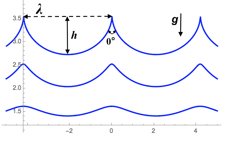
Figure 1: Wave profiles (not to scale) for three values of the dimensionless parameter $ka$ proportional to the wave slope: $ka=0.3678$ (top), $ka=0.3$ (middle) and $ka=0.15$ (bottom). The crest loses its differentiability when $ka=e^{-1}$. The initial phase is $\alpha=0$ and $g=1$.

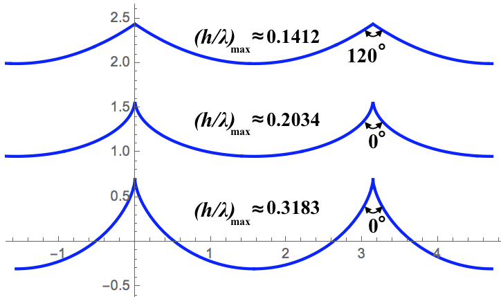
Figure 2: Extreme wave profiles (not to scale) with the same horizontal distance between two successive maxima: Stokes wave (top), real part of $\xi^{\pm}(x,t)$ (middle) and Gerstner wave (bottom). Stokes wave is plotted using a close one-term piecewise approximation suggested in Rainey . Limiting Gerstner wave is an upside-down cycloid.

Discussion.—Asserting the flow of physical interest to be free of rotation, Lamb Lamb and Stokes did not endorse Gerstner’s exact solution as much as naval architects and engineers. In 1847 Stokes proposed an approximate solution for irrotational motion by means of a perturbation series: he sought the free-surface elevation as an infinite Fourier series $\sum_{n=1}^{\infty}a_{n}\cos\left(n(kx-\omega t)\right)$ with unknown coefficients $a_{n}$ and without discussing the convergence properties. The convergence of Stokes’ series for small-amplitude deep water waves was proved by Levi-Civita Levi in 1925. A representation similar to the Stokes’ expansion can be written for the waves studied in this Letter. Indeed, for small values of the parameter $ka$ using the Taylor series of the Lambert function we obtain

$$\mbox{Re}\left(\xi^{\pm}(x,t)\right) =a\cos\beta+ka^{2}\cos(2\beta)+\frac{3}{2}k^{2}a^{3}\cos(3\beta)$$

$$+\frac{8}{3}k^{3}a^{4}\cos(4\beta)+O\left((ka)^{5}\right)$$ (10)

where $\beta=\pm\left(kx\mp\omega t+\alpha\right)$ with $\omega=\sqrt{gk}$. The radius of convergence of the series for $W(z)$ around $z=0$ is precisely equal to $1/e$, i.e. to the value of $ka$ for the wave of greatest height. One can compare expression (Exact solution for progressive gravity waves on the surface of a deep fluid) to the corresponding fourth-order Stokes expansion in deep water

$$\xi(x,t) =a\cos\beta-\left(\frac{1}{2}ka^{2}+\frac{17}{24}k^{3}a^{4}\right)\cos(2\beta)+$$

$$+\frac{3}{8}k^{2}a^{3}\cos(3\beta)-\frac{1}{3}k^{3}a^{4}\cos(4\beta)+O\left((ka)^{5}\right)$$

where the dispersion relation involves the amplitude $\omega^{2}=gk(1+k^{2}a^{2}+\dots)$ (see, e.g., Lamb p. 419).

Stokes theory is limited to small amplitude waves and due to the convergence issues cannot yield the extreme wave for any value of the water depth. Nevertheless, Stokes gave an elegant argument to show that if a cusp is attained in an irrotational flow, then its tangents at the apex necessarily make an angle of $120^{\circ}$. How does this agree with our finding that the sharp-edged extreme wave has an included angle of $0^{\circ}$ at the crest? To answer this question let us switch to a frame moving with the crest and introduce polar coordinates $r$, $\theta$ with the origin at the vertex, i.e. let $x+i(y+k^{-1}W(-ka))=re^{i\theta}$ where $\theta$ is measured from one of the branches of the wave. In the vicinity of the vertex the velocity potential behaves as $\phi\propto r^{n}\cos(n\theta)$ so that the tangential and normal velocity components are $v^{r}\propto r^{n-1}\cos(n\theta)$ and $v^{\theta}\propto r^{n-1}\sin(n\theta)$, respectively. In steady flow, according to the Bernoulli equation we have $v^{2}\propto r$ which implies that $n=3/2$. The normal velocity must vanish for a point on the wave profile and hence $3/2\theta=\pi$, giving the Stokes’ result. However, $\theta=120^{\circ}$ is not the only solution to $v^{\theta}=0$ as the trivial solution $\theta=0^{\circ}$ also satisfies it.

The author is supported by the KAUST Fellowship.

References

- (1) F. Gerstner, Theorie der Wellen, Ann. Phys. 32, 412 (1809); A. Constantin, On the deep water wave motion, J. Phys. A: Math. Gen. 34, 1405 (2001).
- (2) W. J. M. Rankine, On the exact form of waves near the surface of deep water, Phil. Trans. R. Soc. Lond. 153, 127 (1863); W. Froude, On the rolling of ships, Trans. Inst. Naval Arch. 2, 180 (1861); W. J. M. Rankine, On the rolling of ships, Trans. Inst. Naval Arch. 13, 62 (1872).
- (3) R. L. Wiegel and J. W. Johnson, Elements of wave theory, Coast. Eng. Proc. 1, 5 (1950).
- (4) G. G. Stokes, Mathematical and Physical Papers (Cambridge Univ. Press, Cambridge, 1880), Vol. 1, p. 319.
- (5) J. F. Toland, On the existence of a wave of greatest height and Stokes’s conjecture, Proc. Roy. Soc. Lond. Ser. A 363, 469 (1978); J. B. McLeod, The Stokes and Krasovskii conjectures for the wave of greatest height, Stud. Appl. Math. 98, 311 (1997); C. J. Amick, L. E. Fraenkel and J. F. Toland, On the Stokes conjecture for the wave of extreme form, Acta Math. 148, 193 (1982); P. I. Plotnikov, A proof of the Stokes conjecture in the theory of surface waves, Stud. Appl. Math. 3, 217 (2002).
- (6) P. I. Plotnikov and J. F. Toland, Convexity of Stokes waves of extreme form, Arch. Rational Mech. Anal. 171, 349 (2004).
- (7) G. D. Crapper, An exact solution for progressive capillary waves of arbitrary amplitude, J. Fluid Mech. 2, 532 (1957).
- (8) A. Constantin, An exact solution for equatorially trapped waves, J. Geophys. Res.: Oceans 117, C05029 (2012); A. Constantin, Some three-dimensional nonlinear equatorial flows, J. Phys. Oceanogr. 43, 165 (2013); D. Henry, On three-dimensional Gerstner-like equatorial water waves, Phil. Trans. R. Soc. A 376, 20170088 (2017).
- (9) V. E. Zakharov, Stability of periodic waves of finite amplitude on the surface of a deep fluid, J. Appl. Mech. Tech. Phys. 9, 190 (1968).
- (10) Recall that Gerstner waves do not have any explicit representation in Eulerian variables.
- (11) R. S. Johnson, A Modern Introduction to the Mathematical Theory of Water Waves (Cambridge Univ. Press, Cambridge, 1997), p. 102; D. Henry, On Gerstner’s water wave, J. Nonlin. Math. Phys. 15, 87 (2008).
- (12) D. V. Chalikov, Numerical Modeling of Sea Waves (Springer, Cham 2016).
- (13) We use a compact notation in which , for is 1, etc., and subscript 0 corresponds to . The star denotes complex conjugation, is the Fourier transform of and the Dirac delta function is .
- (14) V. P. Krasitskii, On reduced equations in the Hamiltonian theory of weakly nonlinear surface waves, J. Fluid Mech. 272, 1 (1994); M. Stiassnie and L. Shemer, On modifications of the Zakharov equation for surface gravity waves, J. Fluid Mech. 143, 47 (1984); M. Glozman, Y. Agnon and M. Stiassnie, High-order formulation of the water-wave problem, Phys D 66, 347 (1993).
- (15) N. S. Ussembayev, Non-interacting gravity waves on the surface of a deep fluid, arXiv:1903.10854.
- (16) The Hilbert transform is defined by , .
- (17) E. A. Kuznetsov, M. D. Spector and V. E. Zakharov, Formation of singularities on the free surface of an ideal fluid, Phys. Rev. E 49, 1283 (1994).
- (18) M. J. Ablowitz, A. S. Fokas and Z. H. Musslimani, On a new non-local formulation of water waves, J. Fluid Mech. 562, 313 (2006).
- (19) In a two-dimensional setting the vorticity vector is identified with its middle component which is orthogonal to the plane of the flow.
- (20) R. M. Corless et al., On the Lambert -function, Adv. Comp. Math. 5, 329 (1996).
- (21) R. C. T. Rainey and M. S. Longuet-Higgins, A close one-term approximation to the highest Stokes wave on deep water, Ocean Eng. 33, 2012 (2006).
- (22) J. V. Wehausen, E. V. Laitone, Surface Waves in Encyclopaedia of Physics (Springer-Verlag, Berlin, 1960), Vol. 3, p. 744.
- (23) L. W. Schwartz and J. D. Fenton, Strongly nonlinear waves, Ann. Rev. Fluid Mech. 14, 39 (1982).
- (24) H. Lamb, Hydrodynamics (Cambridge Univ. Press, Cambridge, 1975), p. 421.
- (25) T. Levi-Civita, Détermination rigoureuse des ondes permanentes d’ampleur finie, Math. Ann. 93, 264 (1925).