Extraction of ¹²CO and ¹³CO maps from Planck data

Rotational transition lines of CO are one of the major tracers used to study star forming regions and Galactic structures. A large number of observations of CO rotational lines are covering the galactic plane, recently the Planck collaboration release the first full sky coverage of J=1-0, J=2-1, and J=3-2 CO lines at a resolution of 10’, 5’, and 5’ FWHM. However, the measured signal in Planck detectors is integrated over large bandpass $(\Delta\nu)/\nu\simeq 0.2$. Consequently, the derived CO products are composite maps including several rotational lines. In the 100 GHz Planck channel, the two main lines are the J=1-0 transitions of ¹²CO and ¹³CO at 115 and 110 GHz respectively. In the present paper, we present and applied a method to construct separate CO integrated intensity maps for the two isotopes. The measurement of the ¹³CO rotational transitions provide an unprecedented all-sky view of the Galaxy for this isotope.

1 Introduction

This paper describes the construction and validation of full-sky carbon monoxyde (CO) maps for ¹²CO and ¹³CO isotopologues from Planck data.
The interstellar medium (ISM) constitutes about 10-15% of the total mass of the Milky Way. The ISM is a composed by atomic and molecular gas, both contain around 50% of its total mass (see Ferrière, 2001; Cox, 2005, for a review). The cold molecular gas, that represent a small fraction of it, is essentially located close to the Galactic plane. Molecular clouds are hosting star formation, and as such, play a major role in the interstellar matter cycle.
Molecular clouds were discovered via the rotational emission line J=1-0 of carbon monoxide in its fundamental electronic and vibrational levels (Wilson et al., 1970; Penzias et al., 1972). Contrary to the atomic component of the neutral ISM, which is directly observable via the spin-flip HI, 21 cm line, the bulk of molecular hydrogen is not directly observable in molecular clouds. CO is abundant, easily excited by collisions with H₂, and easily observable from the ground, it is therefore considered as a good tracer of the molecular component of the ISM.

Thanks to bandpass differences between Planck bolometers in a given frequency channel, large-scale surveys of J=1-0, J=2-1, and J=3-2 CO lines at a resolution of 10’, 5’, and 5’ FWHM angular resolution have been obtained from the Planck satellite data (Planck Collaboration et al., 2013). However, these CO maps contain several lines, mainly from ¹²CO, but also from ¹³CO, and other lines for the J=3-2 CO map extracted from Planck 353 GHz channel.
Extracting CO maps from Planck data is of interest for handling systematic effect in the map-making of polarized map. The bandpass differences that induce significant variations of the CO transmission in Planck polarized detectors induce confusion between intensity and polarization in the map-making process. Considering that ¹²CO and ¹³CO are emitting lines at different frequencies, their transmissions in Planck detectors is different. Therefore, to properly account for the CO leakage into Planck polarized map both ¹²CO and ¹³CO have to be considered independently.
Large-scale surveys of the J=1-0 line of ¹²CO, but also of ¹³CO, have been carried out with meter-sized radio telescopes. Dame et al. (2001) conducted the most complete ¹²CO(1-0) survey, which covers the Milky Way at Galactic latitudes $\|b\|\leq 30^{o}$, with an effective spatial resolution of $0.5^{\rm o}$. In addition, there exist a wealth of smaller ¹²CO(1-0) and ¹³CO(1-0) line observations (see e.g., Jackson et al., 2006; Ridge et al., 2006; Narayanan et al., 2008).
Observations of CO, for the Orion and Monoceros regions, by Magnani et al. (1985); Hartmann et al. (1998); Magnani et al. (2000) have revealed the existence of molecular clouds at Galactic latitudes up to 55^o. Which implies that the effect of CO on Planck map-making is also present at high galactic latitudes. However, these high-latitude observations provide only a limited view of the $\|b\|>30^{o}$ sky.

The J=1-0 ¹²CO and ¹³CO rotational transition lines lie within the 100 GHz spectral bands of the HFI instrument. In this paper, we extract full-sky ¹²CO and ¹³CO maps for this transition from PLanck-HFI data using a component separation method. The data we used to construct and validate the maps are presented in Sect. 2. In Sect. 3, we provide a description of the methodology used to extract the CO maps. Comparison of these component separated CO maps with ancillary data is detailed in Sect. 4. Uncertainties and foreground contamination on those maps are discussed in Sect. 5 and future improvements for these maps in Sect. 6. Finally, we draw conclusions in Sect. 7.

2 Data

2.1 Planck data

This paper is based on the Planck full mission data release 2(The Planck Collaboration 2015 results I, 2016), it uses the full-sky maps from two detector sets (detset) build from the observation of the sky at 100 GHz, and it uses the type-1 CO public map (Planck Collaboration et al., 2013) derived from Planck release 2 with the MILCA method (Hurier et al., 2013). We used the maps in their HEALPix pixelization from (Górski et al., 2005), with $N_{\rm side}=2048$ (1.7’ arcmin pixels). These maps are given in $K_{\rm CMB}$ units for the temperature detset maps at 100 GHz and in K_RJ.km/s for the type-1 CO map. We also made used of half-mission Planck maps for detector sets. These maps are constructed from subsets of observations and enable the construction of noise maps free from astrophysical emissions. In the following, we assume circular gaussian beams with a FWHM of 9.88’ at 100 GHz to describe the sky signal transfer function.

2.2 Ancillary data

We also made use of additional CO surveys to calibrate Planck response to CO emission and to validate the Planck-data based ¹²CO(J=1-0) and ¹³CO(J=1-0) maps.
In particular, for the calibration of Planck map responses to CO lines we used

• the ¹²CO(J=1-0) by Dame et al. (2001) that cover the entire galactic plane over a band of 4-10 degrees in latitude,

• the ¹²CO(J=1-0) and ¹³CO(J=1-0) Boston University FCRAO Galactic Ring Survey (BU FCRAO GRS, Jackson et al., 2006) mapping part of the galaxy with a 45” angular resolution,

whereas we used

• the FCRAO Ophiuchus and Perseus molecular clouds CO surveys (Ridge et al., 2006) at a 45” angular resolution,

• the FCRAO survey of the Taurus molecular cloud (Narayanan et al., 2008), covering 96 square degrees at a 45” angular resolution,

as reference CO surveys to validate the CO-maps derived from Planck data combining the MILCA Type-1 CO maps with detset maps at 100 GHz. For all these reference CO surveys we consider the CO integrated intensity. We also used the map from Dame et al. (2001) to estimate CO Intensity weighted mean velocity on the line of sight which provides the effective frequency at which is seen the signal in the Planck satellite rest-frame.

3 Methodology

3.1 Data model

Our set of 3 maps (Type-1 CO, detset-1, detset-2): $T_{\rm CO}$, $T_{\rm DS1}$, and $T_{\rm DS2}$ can be modeled as,

$$T_{i}=A^{i}_{{}^{12}{\rm CO}}W_{{}^{12}{\rm CO}}+A^{i}_{{}^{13}{\rm CO}}W_{{}^{13}{\rm CO}}+A^{i}_{100{\rm GHz}}T_{100{\rm GHz}},$$ (1)

with $A^{i}_{X}$ the transmission coefficients of the component $X$ in the map $i$, $W_{{}^{12}{\rm CO}}$ and $W_{{}^{13}{\rm CO}}$ the ${}^{12}{\rm CO}$ and ${}^{13}{\rm CO}$ intensity, and $T_{100{\rm GHz}}$ the sky emission at 100 GHz mainly composed by the CMB, thermal dust, Sunyaev-Zel’dovich effect, synchrotron, and free-free emissions. In our situation, these 100 GHz sky components present the same response in all Planck 100 GHz channel detectors. Thus, we have a set of three maps that are composed of three varying components. By construction the transmission $A^{i}_{100{\rm GHz}}$ is equal to unity for detset maps and null for the type-1 CO map. As a consequence, to remove the 100 GHz sky contribution from the detset maps, we only consider their difference. This detset-difference map is also a CO map, however it present different weighting over the 100-GHz Planck detectors, and is therefore presenting a different response to both ¹²CO and ¹³CO than the official type-1 CO maps. Finally, we have a set of two maps that are described by two components: ¹²CO and ¹³CO.

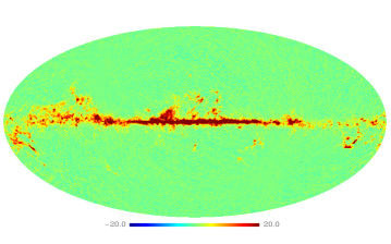
Figure 1: MILCA map of ¹²CO J=1-0 rotational line at 115 GHz reconstructed from Planck detectors at 100 GHz at 30’ FWHM.

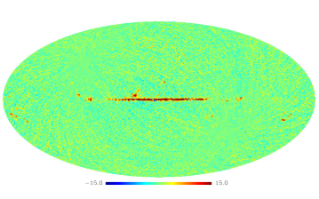
Figure 2: MILCA map of ¹³CO J=1-0 rotational line at 110 GHz reconstructed from Planck detectors at 100 GHz at 30’ FWHM.

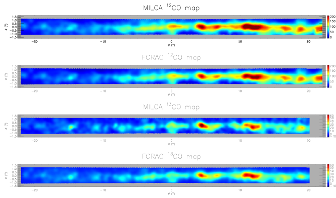
Figure 3: From top to bottom, MILCA, FCRAO ¹²CO maps, MILCA ,and FCRAO ¹³CO maps in K_RJ.km/s units for the Galactic Ring Survey field (Jackson et al., 2006) at 30’ FWHM angular resolution.

3.2 ¹²CO and ¹³CO response in Planck maps

To evaluate the level of both ¹²CO and ¹³CO in the Planck type-1 CO and detset-difference maps, we used Dame et al. (2001) and BU FCRAO GRS data as tracers of ¹²CO and ¹³CO. We describe both the type-1 CO map, $T_{\rm CO}$, and the detset-difference map, $T_{\rm\Delta DS}=T_{\rm DS1}-T_{\rm DS2}$, assuming a parametrization of the form,

$$T_{i}=F^{(i)}_{12}\,{\rm Dame}+F^{(i)}_{13}\,{\rm GRS},$$ (2)

and we derive, trough a linear-fit, $F^{\rm CO}_{12}=0.97\pm 0.01$ and $F^{\rm CO}_{13}=0.47\pm 0.01$ for the type-1 CO map. For the detset-difference map, we obtain $F^{\Delta\rm DS}_{12}=(1.01\pm 0.01)\times 10^{-6}$ K_RJ.km/s/K_CMB and $F^{\Delta\rm DS}_{13}=(1.88\pm 0.01)\times 10^{-6}$ K_RJ.km/s/K_CMB

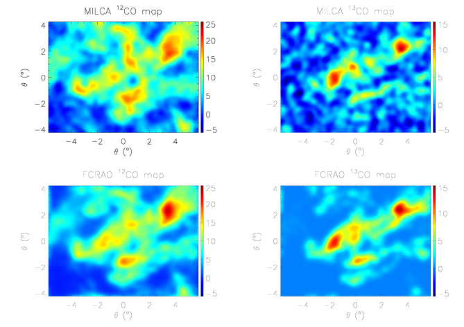
Figure 4: From top to bottom, MILCA, FCRAO ¹²CO maps, MILCA ,and FCRAO ¹³CO maps in K_RJ.km/s units for the Taurus field (Narayanan et al., 2008) at 30’ FWHM angular resolution.

Table 1: Correlation coefficients, uncorrected for instrumental noise covariance, between MILCA CO maps, ancillary observations of CO lines, and thermal dust emission as traced by the Planck 857 GHz channel map.

$\rho$		Tracers
Region	Maps	MILCA 12CO	MILCA 13CO	FCRAO 12CO	FCRAO 13CO	Planck 857 Ghz
Galactic Ring Survey	MILCA 12CO	1.000	0.898	0.996	0.944	0.956
	MILCA 13CO	0.898	1.000	0.929	0.939	0.933
	FCRAO 12CO	0.996	0.929	1.000	0.941	0.951
	FCRAO 13CO	0.944	0.939	0.941	1.000	0.946
Ophiuchus	MILCA 12CO	1.000	0.610	0.940	0.867	0.841
	MILCA 13CO	0.610	1.000	0.791	0.864	0.690
	FCRAO 12CO	0.940	0.791	1.000	0.959	0.893
	FCRAO 13CO	0.867	0.864	0.959	1.000	0.888
Perseus	MILCA 12CO	1.000	0.967	0.961	0.883	0.543
	MILCA 13CO	0.967	1.000	0.749	0.836	0.564
	FCRAO 12CO	0.961	0.749	1.000	0.941	0.596
	FCRAO 13CO	0.883	0.836	0.941	1.000	0.763
Taurus	MILCA 12CO	1.000	0.453	0.939	0.719	0.691
	MILCA 13CO	0.453	1.000	0.672	0.812	0.687
	FCRAO 12CO	0.939	0.672	1.000	0.853	0.758
	FCRAO 13CO	0.719	0.812	0.853	1.000	0.840

3.3 Component separation

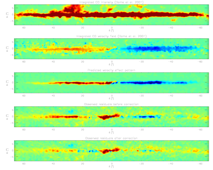
Figure 5: From top to bottom : Integrated intensity CO J=1-0 map from Dame et al. (2001), Integrated velocity field map from Dame et al. (2001), predicted velocity effect pattern, observed residuals between MILCA ¹²CO and Dame et al. (2001) ¹²CO maps before and after correction.

Using the CO spectral responses of our two CO maps (Type-1 CO MILCA map and detset-difference map), we performed a component separation to isolate ¹²CO and ¹³CO. In the present situation the component separation is unique and given by the inversion of the mixing matrix derived in Sect. 3.2. We obtain,

$$W_{{}^{12}{\rm CO}} =1.390\times T_{\rm CO}-3.462\times 10^{5}\times(T_{\rm DS1}-T_{\rm DS2}),$$

$$W_{{}^{13}{\rm CO}} =-0.747\times T_{\rm CO}+7.185\times 10^{5}\times(T_{\rm DS1}-T_{\rm DS2}).$$ (3)

In the following, we refers to this two maps as MILCA-¹²CO and MILCA-¹³CO maps. They are presented on Figures 1 and 2. The two maps are shown at a 30’ FWHM angular resolution to enhance the signal to noise ratio of molecular clouds, especially for the ¹³CO map. We note that the map can be obtained at a resolution of 9.88’ which is the native the angular resolution of the Planck 100 GHz detectors. Considering that these maps have been derived from a single-channel component separation approach, they do not present a significant leakage from other astrophysical components (Planck Collaboration et al., 2013). We observe that the ${}^{13}CO$ emission presents a significantly different spatial distribution than the ¹²CO emission. The ¹³CO is, as expected, mainly observed in regions showing a high ¹²CO emission.

4 Comparison with ancillary data

In this section, we compare our MILCA ¹²CO and ¹³CO maps with well known molecular clouds that have already been observed in both ¹²CO and ¹³CO. We also compare our maps with the thermal dust emission at 857 GHz. Table. 1 summarize the correlation coefficients of the MILCA ¹²CO and ¹³CO with reference CO surveys including the BU FCRAO GRS (Jackson et al., 2006), Ophiuchus, Perseus (Ridge et al., 2006), and Taurus (Narayanan et al., 2008) fields.
We observe that the MILCA-¹²CO and the MILCA-¹³CO present a higher level of correlation with ancillary ¹²CO and ¹³CO data respectively than with thermal dust emission as traced by the Planck 857 GHz channel. By construction, these correlations are expected for the BU FCRAO GRS data that has been used to calibrate the CO transmission within the Planck used in the present analysis. In Fig. 3 we present the comparison of the MILCA and BU FCRAO GRS ¹²CO and ¹³CO maps to illustrate the difference of distribution between ¹²CO and ¹³CO emission.
The other molecular clouds are providing an independent validation that the MILCA ¹²CO and ¹³CO maps are providing a good separation of the two CO isotopes rotational lines. In particular, the Taurus molecular cloud shows a high level of correlation for the ¹³CO, $\rho=0.812$, whereas the correlation between the MILCA ¹³CO and the FCRAO ${}^{12}CO$ map is small $\rho=0.672$. The Taurus field is presented on Fig. 4, it illustrates the significantly different morphologies for the ¹²CO and ¹³CO spatial distributions.
The FCRAO ¹²CO and ¹³CO Taurus maps have a correlation coefficient of $\rho=0.853$, whereas MILCA ¹²CO and ¹³CO Taurus maps have a correlation coefficient of $\rho=0.453$ if not corrected for the instrumental noise covariance and a correlation factor of $\rho=0.886$ when correcting for instrumental noise covariance (see Sect. 5 for a description of the instrumental noise estimation), which is consistent with the value found between the ¹²CO and ¹³CO Taurus maps.
It worth noting that MILCA ¹³CO and the FCRAO ${}^{13}CO$ maps are showing lower correlation factor than their ¹²CO counterpart due to the significantly lower signal-to-noise ratio of the MILCA-¹³CO map.

5 Characterization of the maps

5.1 Uncertainties

In order to estimate uncertainties, we used the so-called half-mission maps to build an astrophysical signal-free map for each data-map,

$$N_{i}=\frac{1}{2}\left(T^{\rm FIRST}_{i}-T^{\rm LAST}_{i}\right),$$ (4)

where, $T^{\rm FIRST}_{i}$ and $T^{\rm LAST}_{i}$ are the map constructed from half-mission subsets of the Planck data.
These maps provides a fair estimation of the noise in Planck full sky maps. Then, we propagate our linear combinations (see Eq. 3.3) of Planck data maps, trough the weights, $w_{i,X}$, to these signal-free maps. We derive CO noise maps,

$$N_{{}^{X}{\rm CO}}=\sum_{i}w_{i,X}N_{i}.$$ (5)

We note that, due to the Planck scanning strategy, the noise is highly inhomogeneous over the sky. To account for this inhomogeneities, we consider the number of observation per pixels $H_{i}$ and we build a variance map for each data map

$$V^{N}_{i}=\frac{<N^{2}_{i}H_{i}>}{H_{i}}$$ (6)

Finally, we propagate these variance maps through our linear combination to deduce CO variance maps,

$$V^{N}_{{}^{X}{\rm CO}}=\sum_{i}w^{2}_{i,X}V^{N}_{i}.$$ (7)

At 10’ FWHM angular resolution, with a pixel size of 1.7’, we obtain an average white noise with a mean standard deviation of 41.2 K_RJ.km/s for the ${}^{12}{\rm CO}$ and 70.2 K_RJ.km/s for the ${}^{13}{\rm CO}$ map.

5.2 CO isotopes residual mixing

The CO transmission in the type-1 CO map and in the detset-difference map have been estimated from the data and are therefore affected by uncertainties. Uncertainties over this transmission coefficients propagate to the weights of the linear combination used to build the MILCA-¹²CO and the MILCA-¹³CO maps. As a consequence, it is expected that the two maps are still presenting some mixing induced by uncertainties over the transmission coefficients. We performed 1000 Monte-Carlo simulations to estimate the expected level of mixing between the ¹²CO and ¹³CO components. We derived a level of mixing of $\sim$1%. Considering that the ¹²CO emission has a higher intensity than the ¹³CO emission (with a typical line ratio of $\sim 0.2$), the ¹²CO is affected by ¹³CO contamination at a $\sim$0.2% level, whereas ¹³CO is affected by ¹²CO emission at a $\sim$5% level. This low-level of contamination is consistent with the ¹²CO and ¹³CO correlation factor in the Taurus field once corrected for instrumental noise covariance, which is consistent with the correlation level of the FCRAO Taurus maps. Leakage between the two component would produce a significantly lower value for this correlation

5.3 Velocity effect

The doppler effect on a CO line induces a modification of the observation frequency, and thus a modification of the effective response induced by the gradient of the CO map effective bandpass. The observed CO integrated intensity in the MILCA maps can be express as,

$$W^{\rm obs}_{\rm CO}=\frac{\left(1+v_{\rm CO}/g\right)}{A_{0}}W^{\rm real}_{\rm CO},$$ (8)

where $g$ is the inverse of the gradient of the bandpass, $A_{0}$ denotes the mismatch on absolute calibration of the map due to non-zero velocity on the line of sight for the sky region (BU FCRAO GRS covered sky) used to calibrate the map, and $v_{\rm CO}$ is the mean velocity of the CO on the line of sight. We construct a map of the CO velocity field from Dame et al. (2001) cube data,

$$W^{\rm obs}_{\rm CO}=\int I_{\rm CO}(u)\,{\rm d}u,$$

$$v_{\rm CO}=\frac{\int u\,I_{\rm CO}(u)\,{\rm d}u}{W^{\rm obs}_{\rm CO}},$$ (9)

where $I_{\rm CO}(u)$ is the CO intensity at a velocity $u$ on the line of sight.

In Fig. 5, we present in the two upper panels the $W^{\rm obs}_{\rm CO}$ and $v_{\rm CO}$ maps computed from Dame et al. (2001) data. In the third panel from the top, we present the predicted pattern of the velocity effect, $R\propto W^{\rm obs}_{\rm CO}\,v_{\rm CO}$, with $R$ the residual emission in the difference map between Dame et al. (2001) and MILCA ¹²CO map. This residual is shown on the antepenultimate panel of Fig. 5.
Finally, we fit the bandpass gradient, $g=(616\pm 1)$ km/s and the calibration mismatch $A_{0}=1.0\pm 0.1$. The bottom panel of Fig. 5 presents the residuals after correction of the velocity effect.

Considering a nearly constant ¹³CO(J=1-0)/¹²CO(J=1-0) ratio in the galactic disc, we can estimate the velocity effect on the MILCA ¹³CO map. The effect for this map is consistent with zero as no clear feature in the ¹³CO(J=1-0)/¹²CO(J=1-0) ratio is correlated to the velocity field.

5.4 Calibration

Using our method, we only have access to CO relative transmission. Consequently, by construction we have the same calibration than Dame et al. (2001) and Jackson et al. (2006) for ¹²CO and ¹³CO respectively.

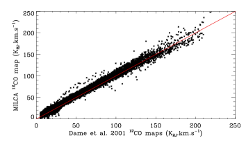
Figure 6: Correlation between MILCA ¹²CO map after correction from velocity effect and Dame et al. (2001) map. The red line shows the 1:1 correlation.

We compute the correlation between MILCA ¹²CO, MILCA ¹³CO and Dame et al. (2001) and BU FCRAO GRS maps.
In Fig. 6, we present the correlation between MILCA ¹²CO and Dame et al. (2001) map after correction of the velocity effect. We observe a 1:1 correlation between the two datasets. In Fig. 7, we also observe a 1:1 correlation between MILCA ¹³CO and BU FCRAO GRS map.

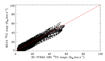
Figure 7: Correlation between MILCA ¹³CO map and BU FCRAO GRS ¹³CO map. The red line shows the 1:1 correlation.

For comparison, we also correlated the MILCA ¹³CO with the Dame et al. (2001) map. We show this correlation in Fig. 8.
We observe, that the relation is not linear. As expected, the faint ¹²CO regions present a low ¹³CO(J=1-0)/¹²CO(J=1-0) ratio, whereas high intensity regions present a higher isotope ratio.

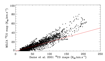
Figure 8: Correlation between MILCA ¹³CO map and and Dame et al. (2001) map. The red line shows a 5:1 slope.

6 Improving the maps in the future

We note that once/if released individual detector maps (or even Time Ordered Information, TOI) at 100 GHz will allow to build CO maps with a lower noise level (An improvement of the order of 20-40% for the noise level compared to the map presented in this paper might be expected and will be determined by the exact distribution of CO transmission coefficients in the 8 Planck detectors at 100 GHz).
An optimal ¹²CO and ¹³CO separation should be performed at the map-making level using a nine components model: I, Q, U stokes parameters for the 100 GHz sky, the ¹²CO and the ¹³CO maps. It will however requires the derivation of the ¹²CO and ¹³CO transmission coefficients for all detectors (8 at 100 GHz) and the gradient of the transmission curves at 110 and 115 GHz for all detectors (to account for transmission variation due the satellite motion with respect to the molecular clouds). The determination of such CO coefficients (16 in totals) will be challenging as it will require to use CO templates at least in intensity and maybe in polarization to avoid biases on those coefficients induced by polarized CO emission (that could be handled by performing the coefficient measurement in low polarized fraction regions).
It is important to precise that for the 100 GHz the possibility of extracting polarized CO emission will be limited by the number of detectors (8) and will require to use the difference of the scanning strategy between Planck surveys 1/3 and 2/4 to be able to have a sufficient number of measurements to extract the 9 components. Otherwise, polarized CO emission would be significantly biased by residual leakage from ¹²CO and ¹³CO intensity. This also imply that for regions of the sky not showing significant difference for the scanning strategy between surveys 1/3 and 2/4 the ¹²CO and ¹³CO polarization will present a very high-level of noise reconstruction.

We also note that the same procedure could be used at 217 and 353 GHz to extract ¹²CO and ¹³CO for the J=2-1 and J=3-2 rotational lines. However, it will also require templates to extract transmission coefficients in the individual detector maps for ¹²CO and ¹³CO separately. The construction of such map will be let for future work.
Finally, it is important to note that the 217 GHz channel is well suited for polarized CO extraction as it possesses 12 detectors (4 unpolarized + 8 polarized) for 9 components (3 intensity + 6 polarization) to extract.
The case of the 353 GHz will be more challenging as thermal dust bandpass mismatch is not negligible, and thus a 12 components (4 intensity + 8 polarization) model is required to describe the 12 detectors (4 unpolarized + 8 polarized), which may lead to very noisy reconstructed maps.

7 Conclusion

We have presented and applied a method to construct separated ¹²CO and ¹³CO maps from public Planck data combining the Type-1 CO MILCA map with detector set maps at 100 GHz. This work present the first full sky cartography for the ¹³CO(J=1-0) line.
We have carefully characterized statistical uncertainties and systematic effect within the map. We also compared our MILCA CO maps with ancillary data. This comparison illustrate that we have effectively separated ¹²CO and ¹³CO. In the future improvements on these maps are expected when all Planck data will be public

References

- Cox (2005) Cox, D. P. 2005, ARA&A, 43, 337
- Dame et al. (2001) Dame, T. M., Hartmann, D., & Thaddeus, P. 2001, ApJ, 547, 792
- Ferrière (2001) Ferrière, K. M. 2001, Reviews of Modern Physics, 73, 1031
- Górski et al. (2005) Górski, K. M., Hivon, E., Banday, A. J., et al. 2005, ApJ, 622, 759
- Hartmann et al. (1998) Hartmann, D., Magnani, L., & Thaddeus, P. 1998, ApJ, 492, 205
- Hurier et al. (2013) Hurier, G., Macías-Pérez, J. F., & Hildebrandt, S. 2013, A&A, 558, A118
- Jackson et al. (2006) Jackson, J. M., Rathborne, J. M., Shah, R. Y., et al. 2006, ApJS, 163, 145
- Magnani et al. (1985) Magnani, L., Blitz, L., & Mundy, L. 1985, ApJ, 295, 402
- Magnani et al. (2000) Magnani, L., Hartmann, D., Holcomb, S. L., Smith, L. E., & Thaddeus, P. 2000, ApJ, 535, 167
- Narayanan et al. (2008) Narayanan, G., Heyer, M. H., Brunt, C., et al. 2008, ApJS, 177, 341
- Penzias et al. (1972) Penzias, A. A., Solomon, P. M., Jefferts, K. B., & Wilson, R. W. 1972, ApJ, 174, L43
- Planck Collaboration et al. (2013) Planck Collaboration, Ade, P. A. R., Aghanim, N., et al. 2013, ArXiv e-prints
- Ridge et al. (2006) Ridge, N. A., Di Francesco, J., Kirk, H., et al. 2006, AJ, 131, 2921
- The Planck Collaboration 2015 results I (2016) The Planck Collaboration 2015 results I. 2016, A&A, 594, A1
- Wilson et al. (1970) Wilson, R. W., Jefferts, K. B., & Penzias, A. A. 1970, ApJ, 161, L43