Relaxation theory for perturbed many-body quantum systems
versus numerics and experiment

Abstract

An analytical prediction is established of how an isolated many-body quantum system relaxes towards its thermal long-time limit under the action of a time-independent perturbation, but still remaining sufficiently close to a reference case whose temporal relaxation is known. This is achieved within the conceptual framework of a typicality approach by showing and exploiting that the time-dependent expectation values behave very similarly for most members of a suitably chosen ensemble of perturbations. The predictions are validated by comparison with various numerical and experimental results from the literature.

The long-standing task to adequately explain the time-dependent relaxation and ultimate equilibration of isolated many-body quantum systems has recently witnessed a veritable renaissance, driven, among others, by very impressive new experimental and numerical capabilities gog16 ; dal16 ; mor18 ; gem04 . On the other hand, quantitative analytical interpretations of the so-acquired data are still rather scarce. For instance, a paradigmatic setup for probing the temporal relaxation behavior of strongly correlated cold atoms was originally proposed in the numerical works cra08 ; fle08 and then experimentally explored in tro12 , concluding that “the exact origin of this enhanced relaxation in the presence of strong correlations constitutes one of the major open problems posed by the results presented here” f1 . The main objective of our Letter is to better understand several such experimental and numerical findings by considering model Hamiltonians of the form

$$H=H_{0}+\lambda V$$ (1)

and asking how the temporal relaxation of the reference system $H_{0}$ is altered by a small perturbation $\lambda V$.

Setting – Given a (pure or mixed) initial state $\rho(0)$, the system (1) evolves in time as $\rho(t)=\mathrm{e}^{-\mathrm{i}Ht}\rho(0)\,\mathrm{e}^{\mathrm{i}Ht}$ ($\hbar=1$), resulting in expectation values $\langle A\rangle_{\!\rho(t)}:=\mbox{Tr}\{\rho(t)A\}$ of an observable (self-adjoint operator) $A$. Of foremost interest to us are the deviations of those $\langle A\rangle_{\!\rho(t)}$ from the corresponding expectation values $\langle A\rangle_{\!\rho_{0}(t)}$ when the same initial state $\rho(0)$ evolves according to the unperturbed Hamiltonian $H_{0}$ in (1).

Denoting by $E_{n}$ and $|n\rangle$ the eigenvalues and eigenvectors of $H$, we assume as usual gog16 ; dal16 ; mor18 ; gem04 that only energies $E_{n}$ within a macroscopically small but microscopically large interval $I:=[E,E+\Delta]$ entail non-negligible level populations $\langle n|\rho(0)|n\rangle$. Put differently, the system must exhibit a macroscopically well-defined energy, while the number of $E_{n}\in I$ is still exponentially large in the degrees of freedom lan70 ; gol10a , and the mean level spacing $\varepsilon$ is approximately constant throughout $I$ gog16 ; dal16 ; mor18 ; gem04 . Very low system energies (close to the ground state) are incompatible with these requirements and are thus tacitly excluded. Finally, $\varepsilon$ is assumed to be (practically) independent of the perturbation strengths $\lambda$ considered in (1). Since the level density $1/\varepsilon$ is – according to the textbook microcanonical formalism – directly connected to the system’s thermodynamics, we thus concentrate on sufficiently weak perturbations in the sense that phase transitions or other significant changes of the thermal equilibrium properties are ruled out.

Next we adopt the common idea of statistical mechanics that the system’s many-body character inevitably implies some uncertainties about the microscopic details. Hence, we temporarily consider an entire class of similar perturbations instead of one particular $V$ in (1). More precisely, denoting by $V^{0}_{\mu\nu}:={{}_{0}\!}\langle\mu\rvert V\lvert\nu\rangle_{\!0}$ the matrix elements of $V$ in the eigenbasis $\lvert\nu\rangle_{\!0}$ of $H_{0}$, we choose an ensemble of matrices whose statistics still reflects the essential properties of the “true” perturbation $V$ in (1) as closely as possible. For instance, if $H_{0}$ models noninteracting particles and $V$ some few-body interactions, the true matrix $V^{0}_{\mu\nu}$ is known to be sparse (most entries are zero) bro81 ; bor16 ; fyo96 ; fla97 . Similarly, the true perturbation may give rise to a so-called banded matrix deu91 ; fyo96 ; fei89 ; wig55 ; gen12 . Accordingly, it is appropriate to work with a possibly (but not necessarily) sparse and/or banded random matrix ensemble.

Denoting ensemble averages by $[\,\cdots]_{V}$, the $V^{0}_{\mu\nu}$’s are considered as unbiased and – apart from $V^{0}_{\nu\mu}=(V^{0}_{\mu\nu})^{\ast}$ – independent random variables, with second moments

$$\left[\lvert V^{0}_{\mu\nu}\rvert^{2}\right]_{\!V}=\sigma_{v}^{2}\,F(\lvert\mu-\nu\rvert)\,,$$ (2)

where the “band profile” $F(n)$ approaches unity for small $n$, and $\sigma_{v}^{2}$ sets the overall scale. Moreover, $F(n)$ is usually a slowly varying function of $n$ and upper bounded by a constant of order unity. In particular, the matrices $V^{0}_{\mu\nu}$ may still be sparse, while $B:=\sum_{n=1}^{\infty}F(n)$ characterizes the bandwidth if the matrix is banded, and $B=\infty$ otherwise. A more detailed discussion is provided in suppl .

Results – Our main result is the following analytical prediction of how the unperturbed behavior $\left\langle A\right\rangle_{\!\rho_{0}(t)}$ is modified by a typical perturbation, i.e., for the vast majority of $V$’s from a given ensemble,

$$\left\langle A\right\rangle_{\!\rho(t)}=\langle A\rangle_{\!\!\;\rm{mc}}+\lvert g(t)\rvert^{2}\left\{\left\langle A\right\rangle_{\!\rho_{0}(t)}-\langle A\rangle_{\!\!\;\rm{mc}}\right\}\ .$$ (3)

Here $\langle A\rangle_{\!\!\;\rm{mc}}$ is the microcanonical expectation value corresponding to the energy window $I$, and $g(t)$ depends on the mean level spacing $\varepsilon$, the coupling $\lambda$, and the properties of the random matrix ensemble from (2). In particular, for sufficiently weak perturbations we find that

$$g(t)=\exp\{-\Gamma t/2\}\ ,\ \ \Gamma:=2\pi\lambda^{2}\sigma_{v}^{2}/\varepsilon\ ,$$ (4)

where “sufficiently weak” means – besides the requirements in “Setting” – that $\Gamma\ll\varepsilon B$. Likewise, we find that

$$g(t)=2J_{1}(\gamma t)/\gamma t\ ,\ \ \gamma:=\sqrt{8B}\,\lambda\sigma_{v}\ ,$$ (5)

for $\gamma\gg\varepsilon B$ (“sufficiently strong” perturbations), where $J_{\nu}(x)$ are Bessel functions of the first kind. In between, $g(t)$ exhibit as transition from (4) to (5) as detailed in suppl .

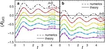
Figure 1: Bosonic Hubbard chain. Dashed: Numerical results from fle08 for the Hubbard model (6) with $L=32$, $J=1$, and various $\lambda:=1/U$, vertically shifted in steps of $-0.25$ for better visibility. The initial state consists of singly occupied even and empty odd sites. The observables are $A:=\hat{n}_{1}$ in (a) and $A:=(\hat{b}^{\dagger}_{1}\hat{b}_{2}-\hat{b}^{\dagger}_{2}\hat{b}_{1})/2\mathrm{i}$ in (b), implying $\langle A\rangle_{\!\!\;\rm{mc}}=1/2$ in (a) and $\langle A\rangle_{\!\!\;\rm{mc}}=0$ in (b). Dash-dotted: Unperturbed analytical solutions $\left\langle A\right\rangle_{\!\rho_{0}\!(t)}=[1-J_{0}(4t)]/2$ in (a) and $\left\langle A\right\rangle_{\!\rho_{0}\!(t)}=J_{1}(4t)/2$ in (b) fle08 . Solid: Eqs. (3), (4) with $\Gamma=4.98\,\lambda^{2}$.

Before turning to their derivation, we further discuss and exemplify those results (3)–(5): So far, these are predictions regarding the vast majority of a given $V$-ensemble. As usual in random matrix theory gol10a ; bro81 ; bor16 ; fyo96 ; wig55 ; deu91 , one thus expects that the “true” (non-random) perturbation $V$ in (1) belongs to that vast majority, provided its main properties are well captured by the considered ensemble. Note that the microscopic dynamics of a many-body system is commonly expected to be extremely sensitive against perturbations (chaotic haa10 ), so that it is virtually impossible to theoretically predict its response exactly or in terms of well-controlled approximations kam71 . Hence, some kind of “uncontrolled” approximation is practically unavoidable. One of them is random matrix theory, which in fact has been originally devised by Wigner for the very purpose of exploring chaotic quantum many-body systems, and is by now widely recognized as a remarkably effective tool in this context haa10 . Another common justification is by comparison with particular examples, to which we now turn. These will be state-of-the-art numerical and experimental results from previous publications, which, however, do not contain the corresponding (numerical) data for the variances required in (2). We will thus concentrate on the weak perturbations regime, where (4) applies. Again, the quantitative values of $\sigma_{v}^{2}/\varepsilon$ required in (4) can in principle be computed, but have not been provided in those publications, and will therefore be treated as fit parameters.

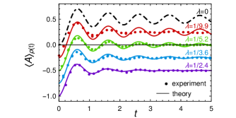
Figure 2: Cold atom experiments. Dots: Experimental data for repulsively interacting Rb atoms in a 1D optical superlattice, adopted from Fig. 2 in tro12 . Initial condition, observable, and dynamics experimentally emulate the theoretical ones from Fig. 1(a). All further details (dash-dotted and solid lines, vertical shifts) are as in Fig. 1.

Examples – Our first example is the numerical exploration by Flesch et al. fle08 (see also cra08 ) of the bosonic Hubbard chain

$$H:=-J\sum_{i=1}^{L}(\hat{b}^{\dagger}_{i+1}\hat{b}_{i}+\hat{b}^{\dagger}_{i}\hat{b}_{i+1})+\frac{U}{2}\sum_{i=1}^{L}\hat{n}_{i}(\hat{n}_{i}-1)$$ (6)

with periodic boundary conditions, creation (annihilation) operators $\hat{b}^{\dagger}_{i}$ ($\hat{b}_{i}$), and $\hat{n}_{i}:=\hat{b}^{\dagger}_{i}\hat{b}_{i}$. For the initial state $\rho(0)$ considered in Ref. fle08 and Fig. 1, the model (6) can be recast as an effective spin-1/2 chain by means of a mapping which becomes asymptotically exact for large interaction parameters $U$ giu13 . In the limit $U\to\infty$, the so-obtained “unperturbed” effective Hamiltonian $H_{0}$ amounts to an XX model. The leading finite-$U$ correction takes the form $U^{-1}H_{1}$, where $H_{1}$ contains nearest neighbor, next-nearest neighbor, as well as three-spin terms giu13 . In other words, $H_{1}$ plays the role of the perturbation $V$ in (1), and $1/U$ that of $\lambda$. Since $\left\langle A\right\rangle_{\!\rho_{0}\!(t)}$ and $\langle A\rangle_{\!\!\;\rm{mc}}$ are known (see fle08 and Fig. 1), the only missing quantity is $\sigma_{v}^{2}/\varepsilon$ in (4), which is, as mentioned above, not provided by fle08 , and hence treated as a fit parameter, yielding $\Gamma=4.98\,\lambda^{2}$. The resulting agreement with the numerics in Fig. 1 speaks for itself.

An experimental realization of (6) by a strongly correlated Bose gas has been explored by Trotzky et al. in Ref. tro12 and is compared in Fig. 2 with our theory (3), (4). Adopting $\Gamma=4.98\,\lambda^{2}$ from before, this amounts to an entirely analytic prediction without any fit parameter. Incidentally, the agreement in Fig. 2 improves as $\lambda$ increases. The same tendency is recovered when comparing the numerical results from Fig. 1(a) with the experimental data, suggesting that the model (6) itself may not capture all experimentally relevant details for large $U$ (small $\lambda$).

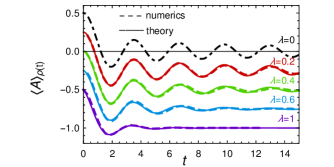
Figure 3: Spin-1/2 XXZ model of the form (1) with $H_{0}:=\sum_{i=1}^{L-1}(S^{x}_{i}S^{x}_{i+1}+S^{y}_{i}S^{y}_{i+1})$, $V:=\sum_{i=1}^{L-1}S^{z}_{i}S^{z}_{i+1}$, observable $A:=\sum_{i=1}^{L}(-1)^{i}S^{z}_{i}/L$, and Néel initial state (see bar09 for more details). Dashed: Numerical results from bar09 for different $\lambda$, vertically shifted in steps of $-0.25$. Dash-dotted: Unperturbed analytical solution $\left\langle A\right\rangle_{\!\rho_{0}\!(t)}=J_{0}(2t)/2$ bar09 . Solid: Eqs. (3), (4) with $\langle A\rangle_{\!\!\;\rm{mc}}=0$, and $\Gamma=0.46\,\lambda^{2}$.

Next we turn to the spin-1/2 XXZ chain with anisotropy parameter $\lambda$ as specified in Fig. 3, exhibiting a gapless “Luttinger liquid” and a gapped, Ising-ordered antiferromagnetic phase for $\lambda\leq 1$ and $\lambda>1$, respectively bar09 . Similarly as before, $\sigma_{\!v}^{2}/\varepsilon$ in (4) is unknown and hence treated as a fit parameter. The analytics in Fig. 3 explains the numerics by Barmettler et al. from Ref. bar09 remarkably well all the way up to the critical point at $\lambda=1$.

Our last example in Fig. 4 is a model of hard-core bosons, numerically explored by Mallayya et al. in Ref. mal19 , and exhibiting so-called prethermalization ber04 ; moe08 ; mor18 for small $\lambda$. Treating $\sigma_{v}^{2}/\varepsilon$ again as a fit parameter, our theory also explains very well such a prethermalization scenario.

For lack of space, further examples have been moved to the Supplemental Material suppl , namely the fermionic systems from Refs. bal15 ; ber16 and a case in which $g(t)$ exhibits a crossover from (4) to (5) without any fit parameters. Moreover, a scaling behavior $\Gamma\propto\lambda^{2}$ as in (4) has also been reported, among others, in Refs. mor18 ; igl11 ; bie17 ; tan18 ; mal18 .

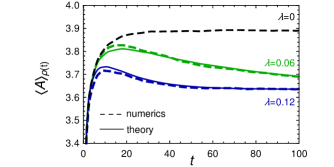
Figure 4: Hard-core boson model of the form (1) with $H_{0}:=\sum_{i}[-\hat{b}_{i}^{\dagger}(\hat{b}_{i+1}+0.7\hat{b}_{i+2})+\mathrm{H.c.}+(\hat{n}_{i}-\frac{1}{2})(\hat{n}_{i+1}+0.7\hat{n}_{i+2}-0.85)]$ and $V:=\sum_{i}[\hat{b}_{i}+\frac{1}{2}(\hat{b}_{i}-b_{i}^{\dagger})\hat{b}_{i+1}+\mathrm{H.c.}]$ (see also (6) and mal19 ). The initial state is thermal with respect to $H_{I}:=H_{0}+\frac{1}{2}\sum_{i}[\hat{b}_{i}^{\dagger}\hat{b}_{i+1}+\mathrm{H.c.}+(\hat{n}_{i}-\frac{1}{2})(\hat{n}_{i+1}-\frac{1}{2})]$, and the observable is $A:=\frac{1}{L}\sum_{i}[\hat{b}^{\dagger}_{i}\hat{b}_{i+1}+\mathrm{H.c.}]$. Dashed: Numerical results from mal19 for different $\lambda$. Solid: Eqs. (3), (4) using the dashed line for $\lambda=0$ as $\left\langle A\right\rangle_{\!\rho_{0}\!(t)}$, the numerical values for $\langle A\rangle_{\!\!\;\rm{mc}}$ quoted in mal19 , and $\Gamma=4.2\,\lambda^{2}$.

Derivation – Adopting the notation as introduced below (1), one readily confirms that

$$\langle A\rangle_{\!\rho(t)}=\sum_{m,n}\mathrm{e}^{\mathrm{i}(E_{n}-E_{m})t}\rho_{mn}(0)A_{nm}\,,$$ (7)

where $\rho_{mn}(t):=\langle m\rvert\rho(t)\lvert n\rangle$ and $A_{nm}:=\langle n\rvert A\lvert m\rangle$. Given that in (7) only levels $E_{n}\in I$ actually matter (see “Setting”), and that their spacings $E_{n+1}-E_{n}$ generically exhibit a Poisson- or Wigner-Dyson-like statistics haa10 of mean value $\varepsilon$, the random fluctuations of those $E_{n+1}-E_{n}$ will also be of order $\varepsilon$ and (practically) uncorrelated. Hence, the $E_{n}-E_{m}$ exhibit typical deviations from their mean value $(n-m)\varepsilon$ of order $|n-m|^{1/2}\varepsilon$. Recalling that $\varepsilon$ is exponentially small lan70 ; gol10a and $|n-m|\varepsilon\simeq|E_{n}-E_{m}|\leq\Delta$, it is reasonable to expect – and justified in more detail in suppl – that the deviations between $(E_{n}-E_{m})t$ and $(n-m)\varepsilon t$ are negligible in (7) for all $t$ of later relevance. Employing this approximation and the unitary basis transformation

$$U_{m\nu}:=\langle m|\nu\rangle_{\!0}$$ (8)

we rewrite (7) in terms of the unperturbed basis $\lvert\nu\rangle_{\!0}$ as

$$\left\langle A\right\rangle_{\!\rho(t)} = \sum_{\mu_{1},\mu_{2},\nu_{1},\nu_{2}}\rho^{0}_{\mu_{1}\nu_{2}}(0)\,A^{0}_{\mu_{2}\nu_{1}}W^{\mu_{1}\mu_{2}}_{\nu_{1}\nu_{2}}(t)\,,$$ (9)

$$W^{\mu_{1}\mu_{2}}_{\nu_{1}\nu_{2}}(t) := \sum_{m,n}\mathrm{e}^{\mathrm{i}(n-m)\varepsilon t}U_{m\mu_{1}}U_{n\mu_{2}}U^{*}_{m\nu_{1}}U^{*}_{n\nu_{2}}\ ,$$ (10)

where $\rho^{0}_{\mu\nu}(0):={{}_{0}\!}\langle\mu\rvert\rho(0)\lvert\nu\rangle_{\!0}$, and $A^{0}_{\nu\mu}:={{}_{0}\!}\langle\nu\rvert A\lvert\mu\rangle_{\!0}$.

The randomness of $V$ (see above (2)) is inherited via (1) by the eigenvector overlaps $U_{m\nu}$ in (8). A particularly important role is played by their second moments, $\left[\lvert U_{m\nu}|^{2}\right]_{\!V}$, which due to (2) only depend on $m-\nu$,

$$\left[\lvert U_{m\nu}|^{2}\right]_{\!V}=:u(m-\nu)\,.$$ (11)

Specifically, the function $g(t)$ from (3) is defined as their Fourier transform,

$$g(t):=\mbox{$\sum_{n}$}\mathrm{e}^{\mathrm{i}n\varepsilon t}\,u(n)\,.$$ (12)

As a first basic result of our present work, we show in suppl that the function $u(n)$ itself follows as $\frac{\varepsilon}{\pi}\lim_{\eta\to 0+}\operatorname{Im}G(n\varepsilon-\mathrm{i}\eta)$ from the ensemble-averaged (scalar) resolvent or Green’s function $G(z)$ of $H$, which in turn can be obtained as the solution of

$$G(z)\left[z-\lambda^{2}\sigma_{v}^{2}\varepsilon^{-1}\mbox{$\int$}G(z-E)\,F(\lvert E\rvert/\varepsilon)\,\mathrm{d}E\right]=1\,.$$ (13)

Along these lines one readily recovers suppl for weak perturbations as specified below (4) the previously known Breit-Wigner distribution wig55 ; deu91 ; fyo96

$$u(n)=\frac{1}{2\pi}\frac{\Gamma/\varepsilon}{(\Gamma/2\varepsilon)^{2}+n^{2}}\,,$$ (14)

with $\Gamma$ from (4), and provided that $\delta:=\varepsilon/\Gamma\ll 1$. Our next goal is to evaluate the ensemble-averaged time evolution (9), hence we need the average of four $U_{m\nu}$’s in (10). The solution of this technically quite challenging problem by means of supersymmetry methods efe83 ; ber10 ; haa10 is provided in the Supplemental Material suppl . There, we also establish that $\delta$ is indeed exponentially small in the system’s degrees of freedom $f$,

$$\delta\approx\exp\{-\mathcal{O}(f)\}\ll 1\,.$$ (15)

Introducing those averages of four $U_{m\nu}$’s into (9) and (10) finally yields

$$[\left\langle A\right\rangle_{\!\rho(t)}]_{V}=\left\langle A\right\rangle_{\!\tilde{\rho}}+\lvert g(t)\rvert^{2}\left\{\left\langle A\right\rangle_{\!\rho_{0}(t)}-\left\langle A\right\rangle_{\!\tilde{\rho}}\right\}+R(t)\ .$$ (16)

Here, $\tilde{\rho}$ is defined via ${{}_{0}\!}\langle\mu\rvert\tilde{\rho}\lvert\nu\rangle_{\!0}:=\delta_{\mu\nu}\sum_{\kappa}\tilde{u}(\nu-\kappa)\rho^{0}_{\kappa\kappa}(0)$ with $\tilde{u}(n):=\sum_{m}u(n-m)u(m)$, essentially amounting to a “washed-out” descendant of the so-called diagonal ensemble (long-time average of $\rho_{0}(t)$) gog16 ; dal16 ; mor18 . Following Deutsch deu91 , $\left\langle A\right\rangle_{\!\tilde{\rho}}$ is thus commonly considered gog16 ; rei15 ; nat18 to closely approximate the microcanonical expectation value $\langle A\rangle_{\!\!\;\rm{mc}}$ (see below (3)). Furthermore, we can infer from  (12), (14), and (15) that $g(t)\simeq\!\int\mathrm{e}^{\mathrm{i}n\varepsilon t}\,u(n)\mathrm{d}n\!=\mathrm{e}^{-\Gamma\lvert t\rvert/2}$, i.e., we recover (4). Finally, the last term in (16) is given by

$$R(t) :=\sum_{\mu,\nu}\rho^{0}_{\mu\mu}(0)\,A^{0}_{\nu\nu}\,r(\lvert t\rvert,\mu-\nu)\,,$$ (17)

$$r(t,n) :=\mathrm{e}^{-\Gamma t}\,\tilde{u}(n)\left\{1-\cos(tn\varepsilon)-\frac{\Gamma\sin(tn\varepsilon)}{n\varepsilon}\right\}.$$ (18)

Due to similar arguments as in the above approximation $\left\langle A\right\rangle_{\!\tilde{\rho}}\simeq\langle A\rangle_{\!\!\;\rm{mc}}$, this term is usually negligibly small. For example, if the unperturbed system satisfies the eigenstate thermalization hypothesis (ETH), the $A^{0}_{\nu\nu}$ are well approximated by $\langle A\rangle_{\!\!\;\rm{mc}}$ deu91 ; sre94 ; rig08 ; dal16 . Observing that $\sum_{n}r(t,n)\!\simeq\!\int r(t,n)\mathrm{d}n\!=\!0$ then immediately implies $R(t)\simeq 0$. However, similar cancellations so that $R(t)\simeq 0$ can be shown to persist under much more general conditions dab20 (some ETH violating examples are also provided above and in suppl ). Altogether, we thus obtain

$$[\left\langle A\right\rangle_{\!\rho(t)}]_{V}=\langle A\rangle_{\!\!\;\rm{mc}}+\lvert g(t)\rvert^{2}\left\{\left\langle A\right\rangle_{\!\rho_{0}(t)}-\langle A\rangle_{\!\!\;\rm{mc}}\right\},$$ (19)

see also Refs. mor18 ; bor16 ; sre99 ; bar08 ; bar09a ; gen13 ; san18 ; kni18 ; rei19 ; nat19 for somewhat similar findings.

The advantage of (19) over (16) is that $\left\langle A\right\rangle_{\!\tilde{\rho}}$ and $R(t)$ are often hard to determine in concrete examples. For the rest – especially if the above approximations leading to (19) might not apply – one also could continue to employ (16) (for an example, see Sec. I B in suppl ).

So far, we focused on sufficiently weak perturbations as specified below (4). Beyond this regime, the solution $G(z)$ of (13) and hence $g(t)$ from (12) will be different, yet we still recovered suppl the same final conclusion as in (19). In particular, for “sufficiently strong” perturbations as specified below (5) one finds wig55 ; fyo96 ; suppl that $u(n)$ approaches a semicircular distribution with radius $\gamma/\varepsilon$ and hence one recovers (5), while in the intermediate regime, $g(t)$ can still be readily obtained by solving (13) numerically.

Our final objective is to quantify the fluctuations $\xi_{V}(t):=\langle A\rangle_{\!\rho(t)}-\left[\langle A\rangle_{\!\rho(t)}\right]_{\!V}$ about the average behavior in terms of the variance $[\xi_{V}^{2}(t)]_{V}$. In view of  (9) and (10), averages over eight $U_{m\nu}$’s are thus required. Referring to suppl for their quite tedious evaluation, we finally obtain the estimate

$$[\xi_{V}^{2}(t)]_{V}\leq c\,\delta\,\|A\|^{2}\ ,$$ (20)

where $\|A\|$ indicates the operator norm and $c$ is some positive real number, which does not depend on any further details of the considered system and is at most on the order of $10^{3}$. Exploiting Chebyshev’s inequality, the probability that $\lvert\xi_{V}(t)\rvert\leq\delta^{1/3}\|A\|$ when randomly sampling $V$’s from the ensemble can thus be lower bounded by $1-\delta^{1/3}c$. In view of (15), the deviations from the average behavior (19) are thus negligibly small for most $V$’s and any preset $t$. Moreover, one can show similarly as in rei16 that for most $V$’s the deviations $\xi_{V}(t)$ must be negligibly small not only for any given $t$, but even for the vast majority of all $t$ within any given time interval $[t_{1},t_{2}]$. Overall, we thus recover our main result from (3).

Conclusions – We derived an analytical prediction for the ensemble-averaged, time-dependent deviations of the perturbed from the unperturbed expectation values in isolated many-body quantum systems. Moreover, we showed that nearly all members of the ensemble behave very similarly to the average. Provided the ensemble has been chosen appropriately, the same behavior is thus typically expected to also apply when dealing with a specific physical model, resulting in our main analytical prediction (3). As a validation, we demonstrated good agreement with a variety of numerical and experimental findings from the literature. Technically speaking, substantial extensions of previously established, non-perturbative supersymmetry methods were indispensable to arrive at those results suppl . Related analytical fyo96 ; fyo95 and numerical rei19 studies suggest that such methods may in the future even be further extended to considerably more general ensembles than those we admitted here. On the conceptual side, a better understanding of when a given physical system is not a typical member of any permitted ensemble kni18 ; rei19a ; ham18 remains as yet another important issue for further studies.

Acknowledgments – Enlightening discussions with Jochen Gemmer and Charlie Nation are gratefully acknowledged. This work was supported by the Deutsche Forschungsgemeinschaft (DFG) within the Research Unit FOR 2692 under Grant No. 397303734.

SUPPLEMENTAL MATERIAL

Throughout this Supplemental Material, equations and figures from the main paper are indicated by an extra letter “m”. For example, “Eq. (m1)” refers to Eq. (1) in the main paper.

Sec. I provides further examples for the applicability of our theoretical prediction (m3). In Sec. II, the arguments below (m7) are elaborated in more detail. Sec. III contains a detailed definition of the considered ensembles of perturbations along with some of their basic properties. In the remaining Secs. IV–VI, we present the derivations of the various moments of eigenvector overlaps $U_{m\nu}:=\langle m|\nu\rangle_{\!0}$ underlying our two key results (m13) and (m20): the supersymmetry calculation for the second and fourth moments in Sec. IV [in particular (m13) and (m14)], a generalized approximation for the fourth and higher such moments in Sec. V, and the evaluation of the eighth moments in Sec. VI [in particular (m20)].

I Further examples

In this section, we compare our main result (m3),

$$\left\langle A\right\rangle_{\!\rho(t)}=\langle A\rangle_{\!\!\;\rm{mc}}+\lvert g(t)\rvert^{2}\left\{\left\langle A\right\rangle_{\!\rho_{0}(t)}-\langle A\rangle_{\!\!\;\rm{mc}}\right\},$$ (1)

with additional numerical examples, namely two fermionic systems in Secs. I.1 and I.2, and a sparse and banded random matrix model in Sec. I.3.

As already pointed out in the main paper, for the numerical results from the literature, with which we compare our analytical prediction (1), the necessary details to determine the function $g(t)$ can in principle be calculated numerically, but they unfortunately have not been provided in the corresponding published works. Therefore, we employ the approximation $|g(t)|^{2}=\mathrm{e}^{-\Gamma t}$, which is theoretically predicted to apply, at least, whenever the perturbation is sufficiently weak (see below (m4)). In the same vein, the quantitative value of the ratio $\sigma_{v}^{2}/\varepsilon$ in our theoretical prediction $\Gamma=2\pi\lambda^{2}\sigma_{v}^{2}/\varepsilon$ from (m4) has not been published in the pertinent numerical works and is therefore treated as a fit parameter.

While the above considerations apply to all the examples from the main paper and also those in Secs. I.1 and I.2 below, for the last example in Sec. I.3 all relevant quantities to determine $g(t)$ in (1) will be exactly known.

I.1 Fermionic Hubbard model

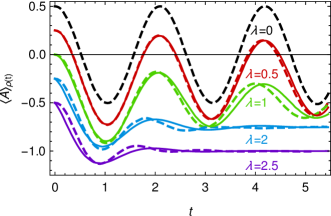
Figure 1: Fermionic Hubbard model. The Hamiltonian $H=H_{0}+\lambda V$ and the observable $A$ are specified by (2) and (3). As detailed in bal15 , the initial state consists of one fermion per site with opposing spins between connected sites. Dashed: Dynamical mean-field theory results, adopted from Fig. 3(a) in bal15 for $\lambda=0,0.5,1,2,2.5$, and vertically shifted in steps of $-0.25$. Solid: Corresponding theoretical prediction (1) with $\left\langle A\right\rangle_{\mathrm{mc}}=0$, $\lvert g(t)\rvert^{2}=\mathrm{e}^{-\Gamma t}$, $\Gamma=0.22\,\lambda^{2}$, and using the numerical results for $\lambda=0$ as $\left\langle A\right\rangle_{\!\rho_{0}\!(t)}$.

We consider the fermionic Hubbard model as studied by Balzer et al. in Ref. bal15 , defined by the Hamiltonian $H=H_{0}+\lambda V$ with

$$H_{0}:=-\sum_{\langle ij\rangle,\sigma}\hat{c}^{\dagger}_{i\sigma}\hat{c}_{j\sigma},\quad V:=\sum_{i}(\hat{n}_{i\uparrow}-\tfrac{1}{2})(\hat{n}_{i\downarrow}-\tfrac{1}{2}),$$ (2)

where $\hat{c}^{\dagger}_{i\sigma}$ ($\hat{c}_{i\sigma}$) creates (annihilates) a fermion with spin $\sigma\in\{\uparrow,\downarrow\}$ at site $i$, and $\hat{n}_{i\sigma}:=\hat{c}^{\dagger}_{i\sigma}\hat{c}_{i\sigma}$. The notation $\sum_{\langle ij\rangle}$ indicates the sum over all pairs of connected sites in a Bethe lattice of infinite coordination number. This model was studied in bal15 using dynamical mean-field theory. The observable

$$A:=\tfrac{1}{2}\langle\hat{c}^{\dagger}_{k}\hat{c}_{\bar{k}}+\hat{c}^{\dagger}_{\bar{k}}\hat{c}_{k}\rangle$$ (3)

measures the correlation between conjugated momentum modes $k$ and $\bar{k}$ (see bal15 for details).

Similarly as for the examples presented in the main paper, we compare the numerics from bal15 to our theoretical prediction (1) with $\lvert g(t)\rvert^{2}=\mathrm{e}^{-\Gamma t}$. Moreover, since the proportionality constant $\sigma_{v}^{2}/\varepsilon$ between $\Gamma$ and $\lambda^{2}$ [cf. Eq. (m4)] is not available from the original publication bal15 , it is again treated as a fit parameter. As Fig. 1 shows, we find good agreement between numerics and theory up to quite large $\lambda$ values. The remaining deviations for large $\lambda$ and small $t$ could hint at a banded structure of the perturbation matrix since the behavior in this regime is seemingly better described by a Bessel-like decay [see (m5) and the discussion between (m19) and (m20) in the main paper as well as the subsequent Sec. I.3 of this Supplemental Material].

I.2 Spinless fermions

Next, we turn to a model of spinless fermions in a periodic one-dimensional lattice, whose Hamiltonian $H=H_{0}+\lambda V$ consists of

$$H_{0} :=-\sum_{i=1}^{L}\left\{\!\left[1+(-1)^{i}\delta\right]\!\left(\hat{c}_{i}^{\dagger}\hat{c}_{i+1}+\hat{c}_{i+1}^{\dagger}\hat{c}_{i}\right)+U\hat{n}_{i}\hat{n}_{i+1}\!\right\}\!,$$ (4a)

$$V :=-\sum_{i=1}^{L}\left(\hat{c}_{i}^{\dagger}\hat{c}_{i+2}+\hat{c}_{i+2}^{\dagger}\hat{c}_{i}\right).$$ (4b)

Here, $c_{i}^{\dagger}$ ($c_{i}$) creates (annihilates) a spinless fermion at site $i$, and $\hat{n}_{i}:=\hat{c}_{i}^{\dagger}\hat{c}_{i}$. Bertini et al. ber16 investigated the effect of the next-nearest neighbor tunneling $V$ on the dynamics by means of equations-of-motion techniques for a lattice of $L=320$ sites. The observable is a tunneling correlation

$$A:=\frac{1}{2}\left(\hat{c}_{L/2}^{\dagger}\hat{c}_{L/2-1}+\hat{c}_{L/2-1}^{\dagger}\hat{c}_{L/2}\right)$$ (5)

and the system is prepared in a thermal state with respect to $H_{0}$ from (4a) with dimerization parameter $\delta=0$ and nearest-neighbor interaction $U=0$ at inverse temperature $2$. Quenching to $\delta=0.1$ and $U=0.4$, the numerical result from ber16 for the unperturbed dynamics ($\lambda=0$) is shown as a dashed black curve in Fig. 2. Since the system is nearly integrable for $\lambda=0$, this dashed black curve settles down to a nonthermal prethermalization plateau within the time scales shown ber16 . Upon activating and increasing $\lambda$, the system departs farther and farther from integrability, and the time-dependent expectation values approach the thermal value better and better for large times.

Yet, as already observed in Ref. ber16 , the numerically approached long-time limit still appears to notably deviate from the thermal value for small $\lambda$, presumably due to the finite system size in combination with the still rather mild integrability breaking, and possibly also due to non-negligible numerical inaccuracies at large times. For this reason, instead of comparing the numerics from ber16 with the analytic approximation from (1), we rather employed – as announced in the main paper below Eq. (m19) – our more general original result from (m16). In doing so, we utilized, as before, the approximations $R(t)=0$ and $\lvert g(t)\rvert^{2}=\mathrm{e}^{-\Gamma t}$, and we fitted the ratio $\sigma_{v}^{2}/\varepsilon$, yielding $\Gamma=0.098\,\lambda^{2}$. Moreover, we again used for the unperturbed behavior $\left\langle A\right\rangle_{\!\rho_{0}\!(t)}$ in (m16) the numerical results for $\lambda=0$ (dashed black line in Fig. 2). But unlike before, we now also treated the long-time limit $\left\langle A\right\rangle_{\!\tilde{\rho}}$ in Eq. (m16) as a fit parameter. The resulting agreement between numerics and analytics in Fig. 2 is very good for all numerically available $\lambda$-values. The actually employed values of $\left\langle A\right\rangle_{\!\tilde{\rho}}$ were $0.232,\,0.230,\,0.223,\,0.207,\,0.199,\,0.199,\,0.199$ for $\lambda=0.25,\,0.32,\,0.375,\,0.425,\,0.5,\,0.55,\,0.6$, respectively. In particular, with increasing $\lambda$ the long-time limit indeed seems to converge towards some constant (presumably thermal) value.

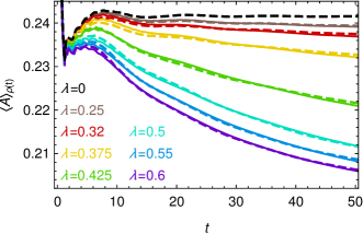
Figure 2: Spinless fermions. The model is described by the Hamiltonian (4), the observable is the correlator (5), and the initial state $\rho(0)\propto\exp[2\sum_{i}(\hat{c}_{i}^{\dagger}\hat{c}_{i+1}+\hat{c}_{i+1}^{\dagger}\hat{c}_{i})]$. Dashed: Numerical equations-of-motion results for various $\lambda$-values, adopted from Fig. 3 in Ref. ber16 . Solid: Corresponding theoretical predictions, as detailed in the main text.

I.3 Sparse and banded random matrix model

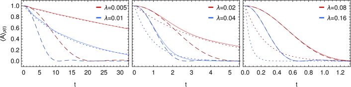
Figure 3: Sparse and banded random matrix model. The unperturbed Hamiltonian $H_{0}$ has eigenvalues $E^{0}_{\mu}=\varepsilon\mu$ with $\varepsilon=1/512$ and $\mu=1,\ldots,16384$. The perturbation $V^{0}_{\mu\nu}$ is a random matrix with sparsity $p=0.8$ and Gaussian distributed nonvanishing entries with mean zero and variance $[\lvert V^{0}_{\mu\nu}\rvert^{2}]_{V}=\sigma_{v}^{2}F(\lvert\mu-\nu\rvert)$, where $\sigma_{v}^{2}=(1-p)=0.2$ and $F(n)=\Theta(B-n)$ with $B=750$. The initial state and observable are $\rho(0)=A=\lvert\mu\rangle_{\!0}{{}_{0}\!}\langle\mu\rvert$ with $\mu=8192$. Accounting for the different time scales, the dynamics for smaller and larger $\lambda$ values are presented in separate plots for better visibility. Solid: Numerically determined $\langle A\rangle_{\!\rho(t)}$. Dotted: Analytical prediction $\left\langle A\right\rangle_{\!\rho(t)}=\lvert g(t)\rvert^{2}$ for the exponential decay (9), following from (1) by exploiting that $\left\langle A\right\rangle_{\!\rho_{0}\!(t)}=1$ and $\langle A\rangle_{\!\!\;\rm{mc}}=1/N\simeq 0$. Dashed: Analytical prediction $\left\langle A\right\rangle_{\!\rho(t)}=|g(t)|^{2}$ for the Bessel-like decay (10). As theoretically predicted, the numerically exact results (solid lines) are well approximated by the dotted lines for $\lambda\ll\lambda_{c}$ and by the dashed lines for $\lambda\gg\lambda_{c}$, where the crossover value $\lambda_{c}\simeq 0.05$ follows from the condition $\Gamma\simeq\gamma$.

In order to have detailed control of all relevant parameters and to obviate any sort of fitting, we finally consider a model of sparse and banded random matrices, which constitutes a direct implementation of the approach from the main paper (see also Sec. III.1 below): The unperturbed Hamiltonian $H_{0}$ consists of equally spaced eigenvalues $E^{0}_{\mu}=\varepsilon\mu$ with level spacing $\varepsilon=1/512$. The matrix elements $V^{0}_{\mu\nu}:={{}_{0}\!}\langle\mu\rvert V\lvert\nu\rangle_{\!0}$ of the perturbation $V$ in the eigenbasis of $H_{0}$ are independent random variables (apart from $(V^{0}_{\mu\nu})^{*}=V^{0}_{\nu\mu}$), distributed as follows: With probability $p=0.8$ we set $V^{0}_{\mu\nu}=0$, so that the matrix is sparse with about $80\,\%$ of the matrix elements vanishing. The nonzero elements, in turn, have Gaussian distributed real and imaginary parts with mean zero and variance $F(\lvert\mu-\nu\rvert)/2$ if $\mu\neq\nu$, while those with $\mu=\nu$ are purely real and of unit variance. For the band profile $F(n)$, we choose a sharp cutoff at $n=B$, i.e., $F(n):=\Theta(B-n)$ with the Heaviside step function $\Theta(x)$. Altogether, we thus obtain the first two moments $[V^{0}_{\mu\nu}]_{V}=0$ and $[\lvert V^{0}_{\mu\nu}\rvert^{2}]_{V}=\sigma_{v}^{2}\,F(\lvert\mu-\nu\rvert)$ with $\sigma_{v}^{2}=1-p=0.2$, corresponding to (m2) in the main paper.

In the numerical example presented in Fig. 3, the total Hilbert space dimension is $N=2^{14}=16384$. For the initial state, we choose the eigenstate $\rho(0):=\lvert\mu\rangle_{\!0}{{}_{0}\!}\langle\mu\rvert$ of the unperturbed system with $\mu=N/2=8192$, i.e., from the middle of the spectrum. As the observable, we choose $A=\rho(0)$, too, measuring the survival probability of the initially populated energy level $\lvert\mu\rangle_{\!0}$. Consequently, the unperturbed time evolution is constant, $\langle A\rangle_{\!\rho_{0}(t)}=1$, while the thermal expectation value is $\langle A\rangle_{\!\!\;\rm{mc}}=1/N\simeq 0$. The theory (1) thus predicts $\langle A\rangle_{\!\rho(t)}=\lvert g(t)\rvert^{2}$ for the perturbed dynamics, where, as in (m12),

$$g(t):=\sum_{n}\mathrm{e}^{\mathrm{i}n\varepsilon t}\,u(n)$$ (6)

is the Fourier transform of $u(n)$ from (m11). As stated in the main paper and derived in Sec. IV.2 below, the function $u(n)$ exhibits a crossover from the Breit-Wigner form (m14) for weak perturbations in comparison with the energy scale of the perturbation bandwidth $\varepsilon B$,

$$u(n)=\frac{1}{2\pi}\frac{\Gamma/\varepsilon}{(\Gamma/2\varepsilon)^{2}+n^{2}},\quad\Gamma:=\frac{2\pi\lambda^{2}\sigma_{v}^{2}}{\varepsilon}\,,$$ (7)

to the semicircular shape [cf. above (m20)] for stronger perturbations,

$$u(n)=\frac{2\varepsilon^{2}}{\pi\gamma^{2}}\sqrt{\frac{\gamma^{2}}{\varepsilon^{2}}\!-\!n^{2}}\,\Theta\!\left(\!\frac{\gamma^{2}}{\varepsilon^{2}}-n^{2}\!\right),\,\gamma:=\sqrt{8B}\,\lambda\sigma_{v}\,.$$ (8)

For the Fourier transform $g(t)$ from (6), this implies a crossover from an exponential decay with rate $\Gamma/2$,

$$g(t)=\mathrm{e}^{-\Gamma\lvert t\rvert/2}\,,$$ (9)

to a Bessel-like decay with rate $\gamma$,

$$g(t)=2J_{1}(\gamma t)/\gamma t\,,$$ (10)

where $J_{1}(x)$ is a Bessel function of the first kind.

Choosing a fixed bandwidth $B=750$, we compare these two theoretical predictions with numerical results for a single realization $V$ of the above specified random matrix ensemble in Fig. 3. We find excellent agreement between the numerics and the exponential decay (9) for sufficiently small values of $\lambda$, and equally splendid agreement between the numerics and the Bessel-like decay (10) for sufficiently large values of $\lambda$. Moreover, the crossover between the two regimes around $\Gamma\simeq\gamma$ is nicely illustrated. Finally, we observe that upon increasing $\lambda$, deviations from the exponential behavior become pronounced at short times first. This can be traced back to the tails of $u(n)$, which begin to decay faster than in the Breit-Wigner distribution (7) when $n$ approaches the bandwidth $B$ fyo96 ; wig55 , i.e., for large $n$, and hence the deviations of the Fourier transform (6) from the behavior in (9) will be most pronounced for small $t$.

Remarkably enough, the deviations for small $t$ appearing at larger perturbations strengths $\lambda$ in the above Fig. 1 as well as (less pronounced) in Figs. m1, m3, and m4 of the main paper seem to be of somewhat similar character as those in Fig. 3, suggesting that they might be caused by a finite bandwidth of the corresponding perturbation matrix $V^{0}_{\mu\nu}$.

II Justification of Eq. (m10)

In this section, additional details regarding the line of reasoning below Eq. (m7) and thus the justification for approximating $(E_{n}-E_{m})t$ in (m7) by $(n-m)\varepsilon t$, leading to Eq. (m10), are provided.

Our starting point is Eq. (m7), i.e.,

$$\langle A\rangle_{\!\rho(t)}=\sum_{m,n}\mathrm{e}^{\mathrm{i}(E_{n}-E_{m})t}\rho_{mn}(0)A_{nm}\,.$$ (11)

As said below (m1), we assume that only energies $E_{n}$ within some macroscopically small but microscopically large interval $I:=[E,E+\Delta]$ exhibit non-negligible populations $\rho_{nn}(0)$ of the corresponding energy eigenstates $|n\rangle$. Accordingly, we approximate all $\rho_{nn}(0)$ with $E_{n}\not\in I$ by zero, and by exploiting the Cauchy-Schwarz inequality $|\rho_{mn}(0)|^{2}\leq\rho_{mm}(0)\rho_{nn}(0)$, we can conclude that only summands with $E_{m},E_{n}\in I$ actually contribute in (11).

Temporarily, we thus restrict ourselves to labels $m$ and $n$ with $E_{m},E_{n}\in I$. Moreover, we assume without loss of generality that the $E_{n}$’s are ordered by magnitude.

Again as said below (m1), we furthermore focus on intervals $I$ so that the (locally averaged) level spacings $E_{n+1}-E_{n}$ are approximately constant throughout $I$, and we denote this constant by $\varepsilon$.

Our next assumption is that the level spacings $E_{n+1}-E_{n}$ exhibit some well-defined statistical distribution, for instance a Poisson or a Wigner-Dyson statistics, or some other (intermediate) statistics with qualitatively similar features. It is well-established haa10 ; bro81 that this assumption can be taken for granted for practically any Hamiltonian $H$. We furthermore assume that the level spacings are statistically independent of each other. Again, it is well-known haa10 ; bro81 that this assumption is generically satisfied in very good approximation, although neighboring level spacings strictly speaking still exhibit some very weak correlations, which further decrease very rapidly with increasing distance between the level pairs. Such correlations could still be included in the subsequent considerations without changing the final conclusions, but for the sake of simplicity we henceforth disregard them.

In other words, the level spacings $E_{n+1}-E_{n}$ are considered as independent, identically distributed random variables with mean value $\varepsilon$. With respect to their variance, one readily sees that, independently of whether we are dealing with a Poisson, a Wigner-Dyson, or some other (reasonable) statistics, the variance is always on the order of $\varepsilon^{2}$. Since the $E_{n+1}-E_{n}$ are independent and identically distributed, it follows that $E_{n}-E_{n_{0}}$ is a random variable with mean value $(n-n_{0})\varepsilon$ and variance of order $|n-n_{0}|\varepsilon^{2}$ for an arbitrary but fixed “reference index” $n_{0}$ (with $E_{n_{0}}\in I$). It follows that $E_{n}+c+\epsilon_{n}=n\varepsilon$, where $c:=n_{0}\varepsilon-E_{n_{0}}$ is an $n$-independent constant and $\epsilon_{n}:=E_{n_{0}}-E_{n}+(n-n_{0})\varepsilon$ is a random variable of mean zero and variance on the order of $|n-n_{0}|\varepsilon^{2}$. Furthermore, since the expectation value in (11) remains unchanged if all energies $E_{n}$ are shifted by the same constant value, we can assume without loss of generality that $c=0$ and thus $E_{n}+\epsilon_{n}=n\varepsilon$.

Next we exploit the following rigorous result, derived in Appendix B of Ref. rei19a : If each $E_{n}$ is changed into $E_{n}+\epsilon_{n}$ then the corresponding change of the expectation value in (11) is upper bounded (in modulus) by $\|A\|\,|t|\max|\epsilon_{n}|$, where $\|A\|$ is the operator norm of $A$. Combining this bound with the considerations in the previous paragraphs, one sees that $\max|\epsilon_{n}|$ will be of the same order as $\max|n-n_{0}|^{1/2}\varepsilon$ and that $\max|n-n_{0}|\varepsilon$ can be upper bounded in very good approximation by $\max|E_{n}-E_{n_{0}}|$ and thus by the width $\Delta$ of the interval $I$. It follows that $\max|\epsilon_{n}|$ is (approximately) upper bounded by $\sqrt{\varepsilon\Delta}$.

Altogether, $(E_{n}-E_{m})t$ can thus be replaced by $(n-m)\varepsilon t$ without any significant change of the expectation value in (11) as long as $t\sqrt{\varepsilon\Delta}\ll 1$. At this point, abandoning our temporary restriction to $E_{m},E_{n}\in I$ is trivial. Finally, since $\varepsilon$ is exponentially small in the systems’s degrees of freedom (see main paper), the latter condition is fulfilled for all $t$ of actual interest later on, i.e., before the expectation value (11) very closely approaches its equilibrium (long-time average) value.

III Perturbation ensembles

In this section, we specify and discuss in detail the ensembles of perturbation matrices considered in the main paper and in the following sections. We recall that we are dealing with isolated quantum many-body systems whose Hamiltonian takes the form

$$H=H_{0}+\lambda V$$ (12)

with a fixed unperturbed Hamiltonian $H_{0}$ and a random perturbation $V$. For the latter, we will define in Sec. III.1 an ensemble of operators in terms of their matrix elements in the basis of $H_{0}$,

$$V^{0}_{\mu\nu}:={{}_{0}\!}\langle\mu\rvert V\lvert\nu\rangle_{\!0}\ ,$$ (13)

whose distribution is motivated by the generic form of “real” perturbations in physical systems, as well as by certain invariance properties of such systems (Sec. III.2). Finally, we will explain in Sec. III.3 that the parameter

$$\delta:=\varepsilon/\Gamma\ ,$$ (14)

as already introduced below Eq. (m14) in the main paper, is generically exponentially small in the system’s degrees of freedom [see also Eq. (m15)], a crucial prerequisite for the applicability of our theory to many-body systems.

III.1 Definition

We consider statistical ensembles of perturbations $V$, where each member of the ensemble is given by a formally infinite-dimensional random matrix (13). The distribution of the matrix elements $V^{0}_{\mu\nu}$ should be chosen such that the main properties of the “true” perturbation are emulated reasonably well. As explained in the main paper, the distribution should allow for potentially (but not necessarily) sparse and/or banded matrices with real- or complex-valued entries bro81 ; bor16 ; fyo96 ; fla97 ; deu91 ; fei89 ; wig55 ; gen12 . As already emphasized, e.g., in Ref. fyo96 , this random matrix approach should be contrasted with the much more common modeling of a Hamiltonian such as $H$ in (12) in terms of a Gaussian orthogonal or unitary ensemble (GOE or GUE haa10 ; bro81 ), which would be entirely inappropriate in the present context.

From a technical point of view, the central objects are the overlaps

$$U_{m\nu}:=\langle m|\nu\rangle_{\!0}$$ (15)

[see (m8)] between the eigenvectors of $H_{0}$ and $H$. More precisely, the essential quantities underlying our central results (m16) and (m20) are averages over four and eight factors of such $U_{m\nu}$, respectively, which in turn build on the average of two such overlaps. This raises the question which of the above exemplified specific features of the $V$ ensemble are relevant with respect to those averages over several $U$ matrix elements.

The simplest connection between the $V$’s and $U$’s is obtained by treating $H$ in (12) in terms of elementary (Rayleigh-Schrödinger) perturbation theory. Quantitatively, such an approach may only lead to useful analytical approximations for exceedingly small $\lambda$ values due to the extremely dense energy eigenvalues of $H_{0}$ (the level spacing decreases exponentially with the system’s degrees of freedom gol10a ; lan70 ) and the concomitant small denominators. Hence, nonperturbative methods will be indispensable for our present purposes. However, qualitatively it is quite plausible on the basis of such a perturbative approach that beyond those extremely small $\lambda$ values, a large number of $V^{0}_{\mu\nu}$’s will appreciably contribute to any given $U_{m\nu}$ or products thereof. It is thus reasonable to expect that some generalized kind of central limit theorem (CLT) may apply, so that only a few basic statistical properties of the $V$’s will be actually relevant for the $U$’s. We point out that all these abstract considerations will become concrete in Sec. IV, in particular Sec. IV.2.

Notably, quite significant correlations between the $V^{0}_{\mu\nu}$ may still be admitted, but like in the CLT, they should be largely irrelevant with respect to the $U$’s. In this spirit, we take for granted that all matrix elements $V^{0}_{\mu\nu}$ can be treated as statistically independent random variables, apart from the trivial constraint $(V_{\mu\nu}^{0})^{\ast}=V_{\nu\mu}^{0}$ since $V$ is Hermitian. Furthermore, we recall that we are working within a macroscopically small but microscopically large energy interval $I:=[E,E+\Delta]$, so that the spectra of $H_{0}$ and $H$ are approximately homogeneous throughout $I$ [see also the discussion below (m1)]. Consequently, for the dynamics, only states with $E^{0}_{\mu}\in I$ are actually relevant. Therefore, we can simply assume an infinite homogeneous spectrum by suitably extending the levels beyond the energy interval $I$. This in turn implies that the statistics of the $V^{0}_{\mu\nu}$ can only depend on the difference $\mu-\nu$, and similarly for the $U_{m\nu}$ [see also (m11) and the discussions above (m2)].

Altogether, it is thus reasonable to expect (and will be further corroborated later) that the most important properties of the $V$ ensemble are its first two moments. Indicating ensemble averages as in the main paper by the symbol $[\,\cdots]_{V}$, we moreover expect them to be expressible as [cf. Eq. (m2)]

$$[V^{0}_{\mu\nu}]_{V} =0\,,$$ (16a)

$$[\lvert V^{0}_{\mu\nu}\rvert^{2}]_{V} =\sigma_{v}^{2}\,F(\lvert\mu-\nu\rvert)=:\sigma_{\mu\nu}^{2}\,.$$ (16b)

Here, the “band profile” function $F(n)$ admits the possibility of banded $V$ matrices. As discussed below Eq. (m2) in the main paper, $\sigma_{v}^{2}$ sets the overall scale, while $F(n)$ should be slowly varying with $n$, normalized so as to approach unity for small $n$, and upper bounded by a constant of order unity for all $n$. Notably, however, $F(n)$ is not required to approach zero for large $n$, i.e., the $V$ matrices generally may, but need not be banded, nor is $F(n)$ required to monotonically decrease.

For the rest, the distribution of the $V^{0}_{\mu\nu}$ will indeed turn out (as anticipated above) to be rather arbitrary provided that the dimension of the pertinent energy interval is sufficiently large (see Sec. IV.2 in particular). We therefore stipulate the probability distributions of the matrix elements $V^{0}_{\mu\nu}$ to be of the explicit general form

$$P_{\mu\nu}(v) := [\delta(V^{0}_{\mu\nu}-v)]_{V}=\tilde{P}_{|\mu-\nu|}(v)\ \ \ (\mu\leq\nu)\ ,\$$ (17)

$$\tilde{P}_{j}(v) = p_{j}\,\delta(v)+(1-p_{j})\,f_{j}\!\left(\frac{v}{\tilde{\sigma}_{j}\sqrt{F(j)}}\right)$$ (18)

with $j\in{\mathbb{N}}_{0}$, $0\leq p_{j}<1$, $\tilde{\sigma}_{j}:=\sigma_{v}/\sqrt{1-p_{j}}$, and where $f_{j}(z)$ are generic probability distributions with vanishing mean and unit variance. For $\mu=\nu$, the argument $v$ in (17) and (18) is understood to be real. For $\mu<\nu$, the argument may be complex or real, depending on whether we are dealing with an ensemble of complex or purely real matrices $V^{0}_{\mu\nu}$ (see also Secs. V.2 and  V.3 below for additional formal details). Moreover, we generally take the corresponding $f_{j}(z)$ with $j\geq 1$ to depend on the absolute value $\lvert z\rvert$ only, an assumption we will elaborate on in the subsequent Sec. III.2 in more detail. Finally, the restriction to indices with $\mu\leq\nu$ in (17) is justified by the fact that $(V_{\mu\nu}^{0})^{\ast}=V_{\nu\mu}^{0}$.

Note that from (17), (18), and the properties of $f_{j}(z)$ one readily recovers the relations (16) for the first two moments. [This is one main reason behind the somewhat involved structure of (18).] While the first two moments (16) are thus directly built into the formal definition of the probability distributions (17) and (18), all their remaining statistical properties are still very general.

In particular, the possibility of sparse matrices is accounted for by the $\delta$-peak in (18). In most cases, one actually expects that the diagonal elements are non-sparse, i.e., $p_{0}=0$, and that all off-diagonal elements exhibit (approximately) the same sparsity, i.e., $p_{j}=p_{1}$ for all $j\geq 1$. In this context, we also recall the definition of the effective bandwidth

$$B:=\sum_{n=1}^{\infty}F(n)$$ (19)

introduced below (m2), implying $B=\infty$ if the matrices are not (or only very weakly) banded.

From the distributions of the individual entries (17), we then obtain the total distribution of the matrix $V$ in the $H_{0}$ eigenbasis,

$$P(V) :=\prod_{\mu\leq\nu}P_{\mu\nu}(V^{0}_{\mu\nu})\ .$$ (20)

Averaging over the ensemble of perturbations means an integral over the probability measure $[\mathrm{d}V]\,P(V)$, where

$$[\mathrm{d}V]:=\left[\prod_{\mu}\mathrm{d}V^{0}_{\mu\mu}\right]\left[\prod_{\mu<\nu}\mathrm{d}V^{0}_{\mu\nu}\,\mathrm{d}V^{0*}_{\mu\nu}\right]$$ (21)

is the Lebesgue measure of all independent entries of $V$ and $\mathrm{d}V^{0}_{\mu\nu}\,\mathrm{d}V^{0*}_{\mu\nu}$ is understood as a shorthand notation for $2\,\mathrm{d}(\textrm{Re}\,V^{0}_{\mu\nu})\,\mathrm{d}(\textrm{Im}\,V^{0}_{\mu\nu})$, and where we tacitly focused on complex-valued $v$ for $\mu\neq\nu$ in (17). Symbolically, taking averages over the $V$ ensemble may thus be written in the two equivalent forms $[\,\cdots]_{V}=\int\,[\mathrm{d}V]\,\cdots\,P(V)$.

III.2 Physical motivation

In the previous section we specified the random matrix ensembles that will be admitted in our subsequent calculations. There, as well as in the main paper, we also argued why and how the investigation of such ensembles may provide insight with respect to our actual objective, namely to describe the effects of some given (non-random) perturbation of the “true” physical system of actual interest.

Here, we further elaborate on such considerations. Specifically, we are concerned with the physical motivation for our assumptions regarding the functions $f_{j}(z)$ in (18). For this purpose, the true (non-random) perturbation of actual interest will be temporarily denoted as $\hat{V}$, while the symbol $V$ is reserved for the members of the considered random ensemble.

Our first observation is that if one takes for granted that the probability distributions in (17) indeed depend only on the differences $|\mu-\nu|$, then those distributions can be estimated from the “empirical distribution” of the true matrix elements $\hat{V}^{0}_{\mu\nu}$ by considering subsets with identical values of $|\mu-\nu|$ within the energy interval $I$. Similarly, the various parameters and functions appearing in (18) can be (approximately) determined. Along this line, the appropriate choice of the random matrix ensemble is thus uniquely fixed by the given $\hat{V}$. Analogously, also some of the further assumptions about this ensemble might be “empirically checked”, for instance the statistical independence of the matrix elements, or the features of $F(n)$. Next we specifically address the assumed properties of the functions $f_{j}(z)$.

According to textbook quantum mechanics, multiplying each eigenvector $\lvert\nu\rangle_{\!0}$ of the unperturbed Hamiltonian $H_{0}$ by a factor of the form $\mathrm{e}^{\mathrm{i}\phi_{\nu}}$ with an arbitrary but fixed phase $\phi_{\nu}$ does not entail any physically observable changes. On the other hand, by doing so, each matrix element $\hat{V}^{0}_{\mu\nu}$ acquires an extra factor $\mathrm{e}^{\mathrm{i}(\phi_{\nu}-\phi_{\mu})}$. If we now choose a basis with an arbitrary but fixed set of randomly generated phases $\phi_{\nu}$, it is quite plausible that the corresponding “empirical distributions” from above will be well approximated for any given index pair $\mu\neq\nu$ by a probability distribution $P_{\mu\nu}(v)$ in (17) which does not depend separately on the real and imaginary parts of $v$, but only on the absolute value $|v|$ (see also Sec. V.3 below). Hence, the same must apply to the functions $f_{j}(z)$ with $j\geq 1$, appearing on the right-hand side of (18).

Note that in the above argument we tacitly assumed that after randomizing the phases of the basis vectors $\lvert\nu\rangle_{\!0}$, a reasonable description of the so-obtained model within the general framework of our present random matrix approach is possible at all.

Once the property that $P_{\mu\nu}(v)$ only depends on $|v|$ is established for one (random) choice of the phases $\phi_{\nu}$, the same property of $P_{\mu\nu}(v)$ (and thus of $f_{j}(z)$) can be readily recovered for any other (random or non-random) choice of the $\phi_{\nu}$. Moreover, the underlying ensemble of random matrices $V^{0}_{\mu\nu}$ must exhibit the following invariance: all its statistical properties remain unchanged when each random matrix element $V^{0}_{\mu\nu}$ of every member of the ensemble is multiplied by a factor $\mathrm{e}^{\mathrm{i}(\phi_{\nu}-\phi_{\mu})}$ for any arbitrary but fixed set of phases $\phi_{\nu}\in[0,2\pi]$.

Essentially, we thus can conclude that if a random matrix approach is possible at all, then focusing on such $V$-ensembles does not amount to any significant loss of generality (see also rei19 ; gen12 ; rei15 ).

Finally, the above invariance of the $V$-ensemble can also be employed to once again recover the relation (16a) for any $\mu\neq\nu$. For a direct numerical verification of this relation by means of a concrete physical model system, see also Ref. beu15 .

As an aside we note that even in case the matrix $\hat{V}^{0}_{\mu\nu}$ of the true perturbation happens to be purely real in some specific basis, one may conjecture that a suitably chosen ensemble with complex-valued off-diagonal elements might still do the job as well as a purely real-valued ensemble (this issue will be continued in Sec. V.2 below).

Turning to the so far excluded case $\mu=\nu$, we first observe that we can always add a trivial constant to the true perturbation $\hat{V}$ such that all the $\hat{V}^{0}_{\nu\nu}$ with the property $E_{\nu}^{0}\in I$ [cf. below (m1)] are zero on average. A similar argument as before may then be invoked: If the true perturbation can be reasonably described within a random matrix approach at all, then only random ensembles which exhibit the property $[V^{0}_{\nu\nu}]_{V}=0$ seem appropriate to faithfully emulate the actual system at hand. One thus can infer that $f_{0}(v)$ in (18) must be a probability distribution with real valued argument $v$ and vanishing first moment. (Note that in the case $j=0$ it is not required that $f_{j}(z)$ should only depend on $|z|$.)

We finally remark that the statistics of the diagonal random matrix elements $V^{0}_{\nu\nu}$ is in fact well-known to be of minor relevance anyway rei19 ; fyo95 .

III.3 Small parameter

A general feature of all the subsequent calculations is that they amount to approximations in which the quantity

$$s:=\max_{n}u(n)$$ (22)

plays the role of a small parameter, i.e., we always assume that $s\ll 1$. Here $u(n)$ is given by (m11), i.e.,

$$u(m-n):=[\lvert U_{mn}\rvert^{2}]_{V}\,.$$ (23)

Our first remark is that the small parameter $\delta$ from (14) [see also below (m14)], which measures the inverse full width at half maximum of $u(n)$ in the weak-perturbation limit, is almost, but not exactly identical to $s$. To be precise, we will find in Sec. IV.2 that the two small parameters are related via

$$\delta=(\pi/2)\,s\ .$$ (24)

Our second remark is that in most cases $u(n)$ is found to assume its maximum at $n=0$ and hence $s=u(0)$. However, exceptions with $s\not=u(0)$ are still possible, as exemplified in Fig. 1 of Ref. fyo96 .

Our next objective is to quantify the “smallness” of $s$ and hence of $\delta$ somewhat more precisely. Quite obviously, the actual value of $s$ depends on many details of the specific model under consideration, hence somewhat more general statements are only possible in terms of nonrigorous arguments and rough estimates.

As mentioned earlier, the mean level spacing $\varepsilon$ is exponentially small in the system’s degrees of freedom lan70 ; gol10a . For a typical macroscopic system with, say, $f=10^{23}$ degrees of freedom, $\varepsilon$ is thus an unimaginably small number (on the corresponding natural energy scale, which usually will be very roughly speaking on the order of $10^{x}$ Joule with $|x|\ll f$). Also for “mesoscopic” systems with considerably less extreme $f$ values (arising for example in cold-atom experiments or in numerical simulations), the level spacing $\varepsilon$ is usually still expected to be extremely small on the natural energy scale of the system at hand.

Since $\sum_{n}u(n)=1$ due to (23), and given (24), it seems reasonable to expect, and will be confirmed by all our particular examples below, that $u(n)$ is generically a rather slowly varying function of its argument $n\in{\mathbb{Z}}$, decaying on a characteristic scale of the order of $s^{-1}$ from its maximal value at $n=0$ towards its asymptotic value zero for $|n|\to\infty$. Moreover, we recall that its Fourier transform $g(t)$ from (6) governs the modification of the temporal relaxation in (m7) due to the perturbation $\lambda V$. We thus can infer from (6) that the characteristic time scale of this modification will be of the order of $s/\varepsilon$, where we are still working in time units with $\hbar=1$ [cf. below (m1)]. Since $\varepsilon$ is exponentially small in the degrees of freedom $f$, also $s$ is expected to be exponentially small in $f$, at least if one disregards extremely weak perturbations, which entail modifications of the relaxation which are themselves exponentially slow in $f$. All these considerations may thus be symbolically summarized like in (m15) as

$$s\approx\exp\{-{\cal O}(f)\}\ll 1\ .$$ (25)

IV Eigenvector correlations from supersymmetry

In this section, we derive the results (m13), (m14), and (8) [see also below (m19)] for the “second moments” (23), as well as the related results for the “fourth moments” $[U_{m\mu_{1}}U_{n\mu_{2}}U^{*}_{m\nu_{1}}U^{*}_{n\nu_{2}}]_{V}$, solving the pertinent random matrix problem by means of supersymmetry methods. We lay out the general procedure in Sec. IV.1 before presenting the explicit calculations for the second and fourth moments in Secs. IV.2 and IV.3, respectively.

Throughout this section we tacitly restrict ourselves to matrices with complex-valued off-diagonals $V^{0}_{\mu\nu}$ [see also the discussion below Eq. (18)]. The case of purely real matrices is recovered by combining the results from fyo96 with the approach from Sec. V below.

IV.1 Outline of the method

In this subsection, we sketch the general methodology on which the more detailed calculations in the subsequent Secs. IV.2 and IV.3 are based.

During most of the actual calculation, we choose a Hilbert space of large, but finite dimension $N$ so that $H_{0}$, $V$, and $H$ in (12) amount to $(N\times N)$ matrices (in the eigenbasis of $H_{0}$). Eventually, we will let $N\to\infty$ while keeping both the perturbation strength $\lambda$ and the average level spacing $\varepsilon$ fixed. In the considered ensemble of these Hamiltonians (12), $H_{0}$ is fixed and $V$ is a Hermitian and possibly sparse and/or banded random matrix distributed according to (20).

Eigenvector overlaps from resolvents.

As pointed out in the main paper and in Sec. III.1 above, the key task is to evaluate the ensemble average over products of $U$ matrix elements (15). Such products can be expressed in terms of the resolvent or Green’s function of the Hamiltonian $H=H_{0}+\lambda V$, defined as the operator

$$\mathcal{G}(z):=(z-H)^{-1}\,.$$ (26)

To do so, we choose an arbitrary but fixed energy level $E_{n}$ of $H$ and consider the matrix element $\mathcal{G}^{0}_{\nu\mu}(E_{n}\pm\mathrm{i}\eta):={{}_{0}\!}\langle\nu\rvert\mathcal{G}(E_{n}\pm\mathrm{i}\eta)\lvert\mu\rangle_{\!0}$, yielding

$$\mathcal{G}^{0}_{\nu\mu}(E_{n}\pm\mathrm{i}\eta)=\sum_{m}\frac{E_{n}-E_{m}\mp\mathrm{i}\eta}{(E_{n}-E_{m})^{2}+\eta^{2}}U_{m\mu}U^{*}_{m\nu}\,.$$ (27)

Next we adopt the assumption that the ensemble-averaged second moments $[U_{m\mu}U^{*}_{m\nu}]_{V}$ are (for arbitrary but fixed $\mu$ and $\nu$) sufficiently slowly varying with $m$, so that the sum over $m$ in (27) can be approximated by an integral, i.e.,

$$[U_{n\mu}U^{*}_{n\nu}]_{V} =\frac{\varepsilon}{2\pi\mathrm{i}}\lim_{\eta\to 0+}[\mathcal{G}^{0}_{\nu\mu}(E_{n}-\mathrm{i}\eta)-\mathcal{G}^{0}_{\nu\mu}(E_{n}+\mathrm{i}\eta)]_{V}$$ (28)

and similarly for higher-order moments. Our justification of this assumption is threefold: (i) Exploiting the assumption, we will later determine an explicit (approximate) expression for $[U_{m\mu}U^{*}_{m\nu}]_{V}$, which indeed turns out to be slowly varying with $m$. Taking for granted that the exact solution for $[U_{m\mu}U^{*}_{m\nu}]_{V}$ is unique and that our approximation is not fundamentally flawed, it follows that we have found a close approximation to the unique exact $[U_{m\mu}U^{*}_{m\nu}]_{V}$. (ii) In numerical examples we always found that $[U_{m\mu}U^{*}_{m\nu}]_{V}$ indeed satisfies the assumption. (iii) In random matrix theory, such assumptions are routinely taken for granted without any further comment, while to our knowledge no counterexample has ever been observed.

According to (28), we thus can express the ensemble-averaged product of two eigenvector overlaps in terms of the advanced and retarded resolvents $\mathcal{G}^{0}_{\nu\mu}(E_{n}-\mathrm{i}\eta)$ and $\mathcal{G}^{0}_{\nu\mu}(E_{n}+\mathrm{i}\eta)$, respectively. Analogously, for the fourth-order moments, we will later combine two such second-order expressions (details will be given in Sec. IV.3).

The advantage of the resolvent formalism is that the matrix elements of $\mathcal{G}(z)$ can be expressed as a Gaussian integral with kernel $\mathcal{G}^{-1}(z)=z-H$. Introducing the abbreviation $z^{\pm}:=E_{n}\pm\mathrm{i}\eta$ with $E_{n}\in\mathbb{R}$ and $\eta>0$ for the argument of the retarded and advanced resolvents, the resolvent matrix element can be written as

$$\mathcal{G}^{0}_{\nu\mu}(z^{\pm}) =\frac{\mp\mathrm{i}\,\det(z^{\pm}-H)}{(\pm 2\pi\mathrm{i})^{N}}\int\left[\prod\nolimits_{\alpha}\mathrm{d}x_{\alpha}\mathrm{d}x_{\alpha}^{*}\right]x_{\nu}x^{*}_{\mu}$$ (29)

$$\quad\times\exp\left\{\pm\mathrm{i}\sum\nolimits_{\alpha,\beta}x^{*}_{\alpha}\left(z^{\pm}\,\delta_{\alpha\beta}-H^{0}_{\alpha\beta}\right)x_{\beta}\right\},$$

where $H^{0}_{\alpha\beta}:={{}_{0}\!}\langle\alpha\rvert H\lvert\beta\rangle_{\!0}$, and the choice of the sign in the exponent ensures convergence since $\eta>0$. The normalization factor $\det(z^{\pm}-H)$, and even more so its average, are in general hard to compute because $z^{\pm}-H$ is a high-dimensional matrix. Nevertheless, it can be expressed conveniently by extending the Gaussian integral to anticommuting numbers.

Supersymmetry method.

Our method of choice for the evaluation of average resolvents uses so-called supersymmetry techniques efe83 ; zuk96 ; mir00 ; ber10 ; haa10 . The underlying concept of graded algebras and vector spaces introduces a set of anticommuting or Grassmann numbers $\chi_{1},\chi_{2},\ldots$ with the defining property that $\chi_{i}\chi_{j}=-\chi_{j}\chi_{i}$ for any two such elements. The above cited references provide an introduction to the linear algebra and calculus on the resulting superspaces.

The crucial observation is that for a Gaussian integral similar to (29), if performed over Grassmannian, anticommuting numbers $\chi_{\alpha}$ and $\chi_{\alpha}^{*}$, we obtain

$$\int\left[\prod\nolimits_{\alpha}\mathrm{d}\chi_{\alpha}\mathrm{d}\chi_{\alpha}^{*}\right]\exp\left\{\mathrm{i}\sum\nolimits_{\alpha,\beta}\chi^{*}_{\alpha}\left(z^{\pm}\,\delta_{\alpha\beta}-H^{0}_{\alpha\beta}\right)\chi_{\beta}\right\}$$ (30)

$$\;=\mathrm{i}^{N}\det(z^{\pm}-H)\,$$

where our normalization for the Grassmann integral is $\int\mathrm{d}\chi\mathrm{d}\chi^{*}\,\chi^{*}\chi=1$. Combining (29) and (30), we can thus write

$$\mathcal{G}^{0}_{\nu\mu}(z^{\pm}) =\frac{\mp\mathrm{i}}{(\mp 2\pi)^{N}}\int\left[\prod\nolimits_{\alpha}\mathrm{d}x_{\alpha}\mathrm{d}x_{\alpha}^{*}\mathrm{d}\chi_{\alpha}\mathrm{d}\chi_{\alpha}^{*}\right]x_{\nu}x^{*}_{\mu}$$ (31)

$$\quad\times\exp\left\{\mathrm{i}\sum\nolimits_{\alpha,\beta}\left[\pm x^{*}_{\alpha}\left(z^{\pm}\,\delta_{\alpha\beta}-H^{0}_{\alpha\beta}\right)x_{\beta}\right.\right.$$

$$\qquad\qquad\qquad\left.\vphantom{\sum\nolimits_{\alpha,\beta}}\left.+\chi^{*}_{\alpha}\left(z^{\pm}\,\delta_{\alpha\beta}-H^{0}_{\alpha\beta}\right)\chi_{\beta}\right]\right\}.$$

To condense the notation, we introduce a supervector $X:=(X_{1}\;\cdots\;X_{N})^{\mathsf{T}}$ with

$$X_{\alpha}:=\left(\begin{matrix}x_{\alpha}\\ \chi_{\alpha}\end{matrix}\right).$$ (32)

In the following, we will refer to the commuting component $X_{\alpha\mathrm{B}}:=x_{\alpha}$ as the bosonic part, and to the anticommuting component $X_{\alpha\mathrm{F}}:=\chi_{\alpha}$ as the fermionic part of the supervector $X_{\alpha}$. Similarly, for a supermatrix $M$, we use the notation $M_{\mathrm{B}\mathrm{B}}$ to address the bosonic-bosonic sector, and consequently $M_{\mathrm{B}\mathrm{F}}$ for the bosonic-fermionic, $M_{\mathrm{F}\mathrm{B}}$ for the fermionic-bosonic, and $M_{\mathrm{F}\mathrm{F}}$ for the fermionic-fermionic sectors. Using the above definition of $X$, we can then express (31) as

$$\mathcal{G}^{0}_{\nu\mu}(z^{\pm})=\mp\mathrm{i}\int\frac{\left[\mathrm{d}X\mathrm{d}X^{*}\right]}{(\mp 2\pi)^{N}}\,x_{\nu}\,x^{*}_{\mu}\,\mathrm{e}^{\mathrm{i}X^{\dagger}\left[\left(z^{\pm}-H\right)\otimes L^{\pm}\right]X}.$$ (33)

Here, $L^{\pm}:=\mathrm{diag}(\pm 1,1)$ and $[\mathrm{d}X\mathrm{d}X^{*}]:=\left[\prod_{\alpha}\mathrm{d}x_{\alpha}\mathrm{d}x_{\alpha}^{*}\mathrm{d}\chi_{\alpha}\mathrm{d}\chi_{\alpha}^{*}\right]$ for short. The Kronecker product in the exponent thus consists of a “Hilbert space” factor $(z^{\pm}-H)$ and a “superspace” factor $L^{\pm}$. In a slight abuse of notation, we will omit the Kronecker products in the following and identify $(z^{\pm}-H)$ and $L^{\pm}$ with their respectively lifted counterparts $(z^{\pm}-H)\otimes\mathbb{1}$ and $\mathbb{1}\otimes L^{\pm}$ on the combined Hilbert-superspace, and similarly for other operators acting trivially on either of the two factor spaces. To obtain the average over all perturbations, we then have to integrate over the distribution (20) of $V$, i.e.

$$[\mathcal{G}^{0}_{\nu\mu}(z^{\pm})]_{V} =\mp\mathrm{i}\int\left[\mathrm{d}V\right]\int\frac{\left[\mathrm{d}X\mathrm{d}X^{*}\right]}{(\mp 2\pi)^{N}}\,P(V)\,x_{\nu}x^{*}_{\mu}\,$$ (34)

$$\qquad\qquad\times\mathrm{e}^{\mathrm{i}X^{\dagger}L^{\pm}\left(z^{\pm}-H_{0}-\lambda V\right)X}.$$

The necessary modifications for the computation of the fourth moments $[U_{m\mu_{1}}U_{n\mu_{2}}U^{*}_{m\nu_{1}}U^{*}_{n\nu_{2}}]_{V}$, involving products of two resolvents, will be further discussed in Sec. IV.3.

Outline of the algorithm.

The general procedure to evaluate expressions like Eq. (34) involves the following steps: First, we integrate over the matrix elements $V^{0}_{\alpha\beta}$ of the perturbation $V$, which can be carried out straightforwardly as the integrals are of Gaussian type due to a (generalized) central limit theorem. The remaining superintegral then involves an exponent of fourth order in the supervector $X$. Therefore, second, we invoke a Hubbard-Stratonovich transformation str57 ; hub59 ; efe83 by introducing an auxiliary integral over a supermatrix. Thereby, we reduce the dependence on $X$ in the exponent to second order. This allows us, third, to perform the (now Gaussian) integral over the supervector $X$. Fourth and last, we evaluate the remaining integral over the Hubbard-Stratonovich supermatrix by means of a saddle-point approximation, making use of the large dimensionality $N$ of the considered Hilbert space. In the end, we thus obtain explicit expressions for (products of) averaged resolvents, which give us access to the averaged eigenvector overlap products according to Eq. (28).

IV.2 Second moment

In this subsection, we derive the nonlinear integral equation (m13), whose solution $G(z)$ gives access to the function $u(n)$ from (23). In addition, we solve the equation explicitly in the limiting cases of weak and stronger perturbations [compared to the scale $\varepsilon B$ set by the perturbation bandwidth, cf. (19)], yielding expressions (7) and (8), respectively, for $u(n)$. To this end, we compute the average of the second moment (28) by calculating the average resolvents (34).

Ensemble average.

Evaluating the ensemble average in Eq. (34) amounts to computing the average

$$\left[\mathrm{e}^{-\mathrm{i}\lambda\,X^{\dagger}L^{\pm}VX}\right]_{\!V}=\left[\mathrm{e}^{-\mathrm{i}\lambda\left[\sum_{\alpha}X^{\dagger}_{\alpha}L^{\pm}X_{\alpha}V^{0}_{\alpha\alpha}+\sum_{\alpha<\beta}(X^{\dagger}_{\alpha}L^{\pm}X_{\beta}+X^{\dagger}_{\beta}L^{\pm}X_{\alpha})(\operatorname{Re}V^{0}_{\alpha\beta})+\sum_{\alpha<\beta}(X^{\dagger}_{\alpha}L^{\pm}X_{\beta}-X^{\dagger}_{\beta}L^{\pm}X_{\alpha})(\mathrm{i}\operatorname{Im}V^{0}_{\alpha\beta})\right]}\right]_{\!V}.$$ (35)

Recalling the definition of $\sigma_{\alpha\beta}$ from (16b), and introducing $Y_{\alpha}:=\sigma_{\alpha\alpha}X^{\dagger}_{\alpha}L^{\pm}X_{\alpha}/2$ and $Y_{\alpha\beta}:=\sigma_{\alpha\beta}X^{\dagger}_{\alpha}L^{\pm}X_{\beta}$, the exponent $X^{\dagger}L^{\pm}VX$ on the left-hand side of (35) can be rewritten as $Z+Z^{\ast}$, where

$$Z:=\sum_{\alpha}Y_{\alpha}\frac{V^{0}_{\alpha\alpha}}{\sigma_{\alpha\alpha}}+\sum_{\alpha<\beta}Y_{\alpha\beta}\frac{V^{0}_{\alpha\beta}}{\sigma_{\alpha\beta}}\ .$$ (36)

In other words, $Z$ amounts to a weighted sum of $N(N-1)/2$ independent random variables $V^{0}_{\alpha\beta}/\sigma_{\alpha\beta}$ of zero mean and unit variance. According to the central limit theorem (cf. also the discussion in Sec. III.1), we can thus conclude that $Z$ approaches, for large $N$, a Gaussian distribution with mean zero and variance $Y^{2}:=\sum_{\alpha}Y_{\alpha}^{2}+\sum_{\alpha<\beta}\lvert Y_{\alpha\beta}\rvert^{2}$, and analogously for $X^{\dagger}L^{\pm}VX=Z+Z^{\ast}$.

Since all random variables $V^{0}_{\alpha\beta}$ only occur in combinations of the form (36) in the average resolvent (34), only the limiting distribution of $Z$ actually matters. Hence, we may approximate the distributions $P_{\mu\nu}(v)$ from Eq. (17) by any other distributions with the same values of the mean and variance (since they lead, for a given $X$, to the same limiting distribution for $Z$). In particular, we may use

$$P_{\alpha\alpha}(v)=\frac{\mathrm{e}^{-v^{2}/2\sigma^{2}_{\alpha\alpha}}}{\sqrt{2\pi}\,\sigma_{\alpha\alpha}}\;\text{and}\;P_{\alpha\beta}(v)=\frac{\mathrm{e}^{-\lvert v\rvert^{2}/\sigma^{2}_{\alpha\beta}}}{\pi(\sigma_{\alpha\beta})^{2}}\;(\alpha<\beta),$$ (37)

approximating each matrix element by a normal distribution (with real argument $v$ for $\alpha=\beta$ and complex $v$ for $\alpha<\beta$). Evaluating the integrals over all $V^{0}_{\alpha\beta}$ ($\alpha\leq\beta$) in (34), which factorize because all matrix elements are independent, we then obtain

$$[\mathcal{G}^{0}_{\nu\mu}(z^{\pm})]_{V} =\mp\mathrm{i}\int\frac{[\mathrm{d}X\mathrm{d}X^{*}]}{(\mp 2\pi)^{N}}\,x_{\nu}x_{\mu}^{*}\,\exp\left\{-\tfrac{\lambda^{2}}{2}\sum\nolimits_{\alpha,\beta}(\sigma_{\alpha\beta})^{2}\,\mathrm{str}\left[X_{\alpha}X_{\alpha}^{\dagger}L^{\pm}X_{\beta}X_{\beta}^{\dagger}L^{\pm}\right]+\mathrm{i}\sum\nolimits_{\alpha}(z^{\pm}-E^{0}_{\alpha})X_{\alpha}^{\dagger}L^{\pm}X_{\alpha}\right\},$$ (38)

where ‘$\mathrm{str}$’ denotes the supertrace, i.e., $\mathrm{str}M=\mbox{Tr}M_{\mathrm{B}\mathrm{B}}-\mbox{Tr}M_{\mathrm{F}\mathrm{F}}$ for a supermatrix $M$.

For later use, we also note here that the integrand is invariant under a transformation $X\mapsto TX$, $X^{\dagger}\mapsto X^{\dagger}T^{\dagger}$ for any (pseudo)unitary $T$ which satisfies $T^{\dagger}L^{\pm}T=L^{\pm}$.

Hubbard-Stratonovich transformation.

Our next step is a supersymmetric Hubbard-Stratonovich transformation str57 ; hub59 ; efe83 to get rid of the fourth-order term in $X$ in the exponent of (38). To do so, we introduce a set of $(2\times 2)$ supermatrices $R_{\alpha}$,

$$R_{\alpha}:=\left(\begin{matrix}r_{\alpha 1}&\rho_{\alpha}\\ \rho^{*}_{\alpha}&\mathrm{i}r_{\alpha 2}\end{matrix}\right),$$ (39)

with real numbers $r_{\alpha 1}$, $r_{\alpha 2}$ and anticommuting $\rho_{\alpha}$, $\rho^{*}_{\alpha}$. The choice of an imaginary $\mathrm{F}\mathrm{F}$ entry ensures convergence of the following integral. Namely, the Hubbard-Stratonovich transformation is then based on the identity haa10

$$\int\frac{[\mathrm{d}R]}{(2\pi)^{N}}\exp\left\{-\sum\nolimits_{\alpha,\beta}\tfrac{(\sigma^{-2})_{\alpha\beta}}{2\lambda^{2}}\mathrm{str}\left(R_{\alpha}R_{\beta}\right)\right.$$ (40)

$$\qquad\qquad\qquad\qquad\left.\vphantom{\sum\nolimits_{\alpha,\beta}\tfrac{(\sigma^{-2})_{\alpha\beta}}{2\lambda^{2}}}+\mathrm{i}\sum\nolimits_{\alpha}\mathrm{str}\left(R_{\alpha}X_{\alpha}X_{\alpha}^{\dagger}L^{\pm}\right)\right\}$$

$$\quad=\exp\left\{-\sum\nolimits_{\alpha,\beta}\tfrac{\lambda^{2}(\sigma_{\alpha\beta})^{2}}{2}\mathrm{str}\left(X_{\alpha}X^{\dagger}_{\alpha}L^{\pm}X_{\beta}X^{\dagger}_{\beta}L^{\pm}\right)\right\}\,,$$

where $\sigma^{-2}$ is the inverse of the Hilbert space matrix $\sigma^{2}$ with entries $(\sigma^{2})_{\alpha\beta}:=(\sigma_{\alpha\beta})^{2}$. Moreover, $[\mathrm{d}R]:=\prod_{\alpha}\mathrm{d}R_{\alpha}$ denotes the collective measure of all $R_{\alpha}$ with $\mathrm{d}R_{\alpha}=\mathrm{d}r_{\alpha 1}\mathrm{d}r_{\alpha 2}\mathrm{d}\rho_{\alpha}\mathrm{d}\rho^{*}_{\alpha}$. Substituting (40) into (38), we obtain

$$[\mathcal{G}^{0}_{\nu\mu}(z^{\pm})]_{V} =\mp\mathrm{i}\int\frac{[\mathrm{d}R]}{(2\pi)^{N}}\int\frac{[\mathrm{d}X\mathrm{d}X^{*}]}{(\mp 2\pi)^{N}}\,x_{\nu}x^{*}_{\mu}\exp\left\{-\sum\nolimits_{\alpha,\beta}\!\!\frac{(\sigma^{-2})_{\alpha\beta}}{2\lambda^{2}}\mathrm{str}(R_{\alpha}R_{\beta})+\mathrm{i}\sum\nolimits_{\alpha}X^{\dagger}_{\alpha}L^{\pm}\left(R_{\alpha}+z^{\pm}-E^{0}_{\alpha}\right)X_{\alpha}\right\}.$$ (41)

Comparing (38) and (41), we observe that the Hubbard-Stratonovich transformation essentially identifies $R_{\alpha}\sim X_{\alpha}X^{\dagger}_{\alpha}L^{\pm}$. The integral over the supervector $X$ in (41) now has a Gaussian structure. Therefore, we can evaluate it straightforwardly to find

$$[\mathcal{G}^{0}_{\nu\mu}(z^{\pm})]_{V} =\delta_{\mu\nu}\int\frac{[\mathrm{d}R]}{(2\pi)^{N}}\,\left[\left(R_{\mu}+z^{\pm}-E^{0}_{\mu}\right)^{-1}\right]_{\mathrm{B}\mathrm{B}}\exp\left\{-\mathrm{str}\left[\sum\nolimits_{\alpha,\beta}\tfrac{(\sigma^{-2})_{\alpha\beta}}{2\lambda^{2}}R_{\alpha}R_{\beta}+\sum\nolimits_{\alpha}\ln\left(R_{\alpha}+z^{\pm}-E^{0}_{\alpha}\right)\right]\right\}.$$ (42)

Saddle-point approximation.

Keeping in mind the huge dimension $N$ of the considered Hilbert space and the fact that we will eventually take the limit $N\to\infty$, the remaining integral over the supermatrices $R_{\alpha}$ can be evaluated using a saddle-point approximation ben99 ; mir00 ; haa10 . The reason is that the exponent in (42) is a sum of $N$ very similar terms, so that the exponential is strongly peaked around the global maximum of the real part of its argument and/or highly oscillatory except at points where its imaginary part becomes stationary. Hence the dominant contributions arise from the steepest saddle points in the complex, multidimensional $R$ plane, where the first variation of the exponent vanishes. Computing this first variation and multiplying by the matrix $\lambda^{2}\sigma^{2}$, we obtain the saddle-point equation

$$R_{\mu}+\lambda^{2}\sum_{\alpha}(\sigma_{\mu\alpha})^{2}\left(R_{\alpha}+z^{\pm}-E^{0}_{\alpha}\right)^{-1}=0\,.$$ (43)

To find the saddle points, we first look for diagonal solutions of this equation and consider one component $\hat{R}(E^{0}_{\mu},z^{\pm})$ of $R_{\mu}$, explicitly indicating the dependence of the solution on both the unperturbed and perturbed energy levels. Any further solutions can be generated from diagonal ones by means of the (pseudo)unitary symmetry transformation introduced below (38) haa10 . Next, we substitute the variances $(\sigma_{\alpha\beta})^{2}$ from (16b) with $F(n)$ as specified there, and we make use of the assumption that the energy levels are very dense and approximately uniformly distributed, so that the density of states is essentially $\varepsilon^{-1}$ [cf. discussion below (m1)]. Provided that the summands on the left-hand side of (43) are slowly varying with $\alpha$, which – as will become clear below – is satisfied for $\delta\ll 1$ [cf. Eq. (m15) and Sec. III.3], we can approximate the sum by an integral and arrive at

$$\hat{R}(E^{0}_{\mu},z^{\pm})+\int\frac{\mathrm{d}E}{\varepsilon}\,\frac{\lambda^{2}\sigma_{v}^{2}\,F(\lvert E/\varepsilon-\mu\rvert)}{z^{\pm}-E+\hat{R}(E,z^{\pm})}=0\,.$$ (44)

In fact, given the assumed homogeneity of the spectrum, the solution will only depend on the energy difference $z^{\pm}-E^{0}_{\mu}$, i.e., $\hat{R}(E_{\mu}^{0},z^{\pm})$ can be rewritten in the form $\hat{R}(z^{\pm}-E^{0}_{\mu})$. This simplifies the equation further, resulting in the convolution-type relation

$$\hat{R}(z^{\pm})+\int\frac{\mathrm{d}E}{\varepsilon}\,\frac{\lambda^{2}\sigma_{v}^{2}\,F(\lvert E\rvert/\varepsilon)}{z^{\pm}-E+\hat{R}(z^{\pm}-E)}=0\,.$$ (45)

Note that the sign of the imaginary part of $\hat{R}(z^{\pm})$ has to match the sign of the imaginary part of $z^{\pm}$, $\operatorname{sgn}\operatorname{Im}\hat{R}(z^{\pm})=\pm 1$, for otherwise the integrand in (45) develops a pole. Anticipating the final structure of $[\mathcal{G}^{0}_{\nu\mu}(z^{\pm})]_{V}$ from (42), we introduce the function

$$G(z):=[z+\hat{R}(z)]^{-1}\,,$$ (46)

for which, consequently, $\operatorname{sgn}\operatorname{Im}G(z^{\pm})=\mp 1$ must hold. Substituting into (45), we find that it satisfies

$$G(z^{\pm})\left[z^{\pm}-\frac{\lambda^{2}\sigma_{v}^{2}}{\varepsilon}\int\mathrm{d}E\;G(z^{\pm}-E)\,F(\lvert E\rvert/\varepsilon)\right]=1\,,$$ (47)

which is Eq. (m13) from the main paper. Assuming that $G(z)$ solves (47), we immediately find a diagonal solution

$$R_{*\mu}:=\left[G(z^{\pm}-E^{0}_{\mu})^{-1}-(z^{\pm}-E^{0}_{\mu})\right]\mathbb{1}$$ (48)

of the saddle-point equation (43). As mentioned below (43), any further solutions of the saddle-point equation can be generated from the diagonal one by means of symmetry transformations $T$ satisfying $T^{\dagger}L^{\pm}T=L^{\pm}$. From the Hubbard-Stratonovich transformation (40), we understand that the supermatrix $R$ transforms as $R\mapsto TRT^{-1}$ under this symmetry. But since the solution $R_{*\mu}$ from (48) is proportional to the unit matrix, all transformed solutions collapse back onto the diagonal one, so that this is indeed the only solution of (43). We remark that this will be manifestly different when computing the fourth moment in Sec. IV.3. Furthermore, one also verifies straightforwardly that the second variation of the exponent in (42) with respect to $R_{\mu}$ is proportional to the unit matrix upon substitution of $R_{*\mu}$. Therefore, its superdeterminant is unity and the saddle-point approximation of the integral (42) is obtained from its integrand by plugging in the solution (48) for $R_{\mu}$, so that

$$[\mathcal{G}^{0}_{\nu\mu}(z^{\pm})]_{V}=\delta_{\mu\nu}\,G(z^{\pm}-E^{0}_{\mu})\,.$$ (49)

Hence the function $G(z)$ is appropriately described as the scalar average resolvent. Using $E_{n}-E^{0}_{\mu}\simeq(n-\mu)\varepsilon$ [see below (m1)] and (28), and remembering that $z^{\pm}=E_{n}\pm\mathrm{i}\eta$, we then find

$$[U_{n\mu}U^{*}_{n\nu}]_{V}=\delta_{\mu\nu}\,u(n-\mu)$$ (50)

with

$$u(n):= \,\frac{\varepsilon}{2\pi\mathrm{i}}\lim_{\eta\to 0+}\left[G(n\varepsilon-\mathrm{i}\eta)-G(n\varepsilon+\mathrm{i}\eta)\right]$$ (51)

$$= \,\frac{\varepsilon}{\pi}\lim_{\eta\to 0+}\operatorname{Im}G(n\varepsilon-\mathrm{i}\eta)\,.$$

Here, the last equality follows from $\mathcal{G}(z^{*})=\mathcal{G}(z)^{\dagger}$ [see (26)], and hence, due to (49), $G(z^{*})=G(z)^{*}$. This establishes the results around Eq. (m13) from the main paper.

The remaining task is to solve the defining equation (47) for the scalar average resolvent $G(z)$. Unfortunately, no general solution to this nonlinear integral equation is known to us. However, analytic solutions are available in the limiting cases of weak and strong perturbations compared to the scale $\varepsilon B$ of its bandwidth (19).

Weak perturbations.

Provided that $G(z)$ in Eq. (47) decays much faster than $F(\lvert E\rvert/\varepsilon)$ (which we will verify self-consistently in the end), we can neglect the band profile in the integral altogether and approximate $F(\lvert E\rvert/\varepsilon)\approx 1$ (by normalization), leading to

$$\int\mathrm{d}E\;G(z^{\pm}-E)F(\lvert E\rvert/\varepsilon)\approx\int\mathrm{d}E\;G(E\pm\mathrm{i}\eta)=:C^{\pm}\,.$$ (52)

From the full equation (47), we then obtain

$$G(z^{\pm})=\frac{1}{z^{\pm}-\lambda^{2}\sigma_{v}^{2}C^{\pm}/\varepsilon}\,.$$ (53)

Next, we substitute this functional form back into (52) to determine the constant $C^{\pm}$. The resulting integral needs to be evaluated in the principal-value sense, indicated by the symbol “$\mathrm{PV}$” in the following. For $\eta>0$, this leads to

$$C^{\pm}=\mathrm{PV}\int\mathrm{d}E\;G(E\pm\mathrm{i}\eta)=\mp\mathrm{i}\pi\,.$$ (54)

With (53), we thus find that the average scalar resolvent in the weak-perturbation or large-bandwidth limit is given by

$$G(z^{\pm})=\frac{1}{z^{\pm}\pm\mathrm{i}\Gamma/2}$$ (55)

with $\Gamma=2\pi\lambda^{2}\sigma_{v}^{2}/\varepsilon$ from (7). Together with (51), this proves the result (7) and hence (m14). The self-consistency condition for the weak-perturbation approximation, meaning that $G(z)$ is decaying much faster than the band profile $F(\lvert E\rvert/\varepsilon)$, becomes $\Gamma\ll\varepsilon B$ as stated below Eq. (m4), provided that $F(n)$ remains of order unity for $n\lesssim B$.

Finally, as a technical remark, we note that the solution (48) with $G(z)$ from (55) does not lie on the original contour of integration in (40), see also (39). However, the contour can be adjusted accordingly by shifting $r_{1}\mapsto r_{1}\pm\mathrm{i}\Gamma/2$, which is allowed because the poles in the integrand at $r_{1}=E^{0}_{\alpha}-z^{\pm}$ all lie on the same side of the real axis, below it for ‘$+$’ and above it for ‘$-$’, respectively.

Stronger perturbations.

In the opposite limiting case, when the band profile $F(\lvert E\rvert/\varepsilon)$ decays much faster than the solution $G(z)$ of (47), we can approximate $G(z^{\pm}-E)$ in the integrand by its central value $G(z^{\pm})$. Using the definition (19) of the effective bandwidth, we then find

$$\gamma^{2}\,G(z^{\pm})^{2}/4-z^{\pm}\,G(z^{\pm})+1=0\,,$$ (56)

where $\gamma=\sqrt{8B}\,\lambda\sigma_{v}$ was defined as in (8). Solving this algebraic equation, we immediately obtain

$$G(z^{\pm})=\frac{2}{\gamma^{2}}\left(z^{\pm}\mp\mathrm{i}\sqrt{\gamma^{2}-(z^{\pm})^{2}}\right),$$ (57)

where we already incorporated the requirement that the imaginary parts of $G(z^{\pm})$ and $z^{\pm}$ should have opposite signs [see below (46)]. Together with (51), we then recover (8) and hence the result stated below (m19) for $u(n)$ in the limit of a dominating overlap scale compared to the bandwidth. More precisely, this latter assumption is verified self-consistently if $\gamma\gg\varepsilon B$, as stated below (m5) in the main paper.

IV.3 Fourth moment

In this subsection, we evaluate the fourth moments $[U_{m\mu_{1}}U_{n\mu_{2}}U^{*}_{m\nu_{1}}U^{*}_{n\nu_{2}}]_{V}$ of eigenvector overlaps when the perturbation strength is weak compared to its bandwidth, which is the physically most relevant case for generic many-body systems. More precisely speaking, we will derive the following results:

$$[U_{m\mu_{1}}U_{n\mu_{2}}U^{*}_{m\nu_{1}}U^{*}_{n\nu_{2}}]_{V}$$ (58a)

$$\;=\delta_{\mu_{1}\nu_{1}}\delta_{\mu_{2}\nu_{2}}\,d^{mn}_{\mu_{1}\mu_{2}}+\delta_{\mu_{1}\nu_{2}}\delta_{\mu_{2}\nu_{1}}\left(\delta_{mn}\,d^{mn}_{\mu_{1}\mu_{2}}+f^{mn}_{\mu_{1}\mu_{2}}\right)$$

with

$$d^{mn}_{\mu_{1}\mu_{2}} :=u(m-\mu_{1})\,u(n-\mu_{2})\ ,$$ (58b)

$$f^{mn}_{\mu_{1}\mu_{2}} :=-\left(\tfrac{\Gamma/\varepsilon}{4\pi}\right)u(m-\mu_{1})\,u(n-\mu_{2})$$ (58c)

$$\times\frac{(\Gamma/\varepsilon)^{2}+(\mu_{1}\!-\!\mu_{2})^{2}+(m\!-\!n)^{2}-(\mu_{1}\!+\!\mu_{2}\!-\!m\!-\!n)^{2}}{\left[(m-\mu_{2})^{2}+(\Gamma/2\varepsilon)^{2}\right]\left[(n-\mu_{1})^{2}+(\Gamma/2\varepsilon)^{2}\right]}$$

to leading order in the small parameter $s$ from (22). As some of the steps are straightforward generalizations of the calculation of the second moment in Sec. IV.2, the presentation will be tightened in these places. Moreover, we immediately assume a normal distribution (37) for the perturbation matrix elements $V^{0}_{\mu\nu}$ because the general case of sparse and banded perturbations can be reduced to this effective model as sketched in Sec. IV.2. Focusing, as announced above, on the weak-perturbation/large-bandwidth limit, which essentially amounts to a constant band profile (cf. Sec. IV.2), we will assume right from the beginning that the variance $(\sigma_{\mu\nu})^{2}=\sigma_{v}^{2}=1$ for all $V^{0}_{\mu\nu}$ and control the interaction strength by the parameter $\lambda$.

Figure 4: Fourth moments $[U_{n_{1}\mu_{1}}U_{n_{2}\mu_{2}}U^{*}_{n_{1}\nu_{1}}U^{*}_{n_{2}\nu_{2}}]_{V}$ for various combinations of fixed and variable indices as indicated in the respective panels. Solid: Analytical approximation from  (58). Dots: Numerical averages over $10^{5}$ randomly sampled perturbation matrices $V^{0}_{mn}$. The considered random matrix model is of the form (12), where $H_{0}$ exhibits $N=512$ equidistant levels with level spacing $\varepsilon=1$. The matrix elements $V_{mn}^{0}$ are independent random variables (apart from $(V_{mn}^{0})^{\ast}=V_{nm}^{0}$). The diagonal elements $V^{0}_{nn}$ are Gaussian distributed with zero mean and unit variance. For $m<n$, the real and imaginary parts of $V_{mn}^{0}$ are independent Gaussian distributed random variables with mean zero and variance $1/2$. The perturbation strength is $\lambda=1.33$, implying $\sigma_{v}^{2}=1$, $\Gamma\simeq 11$, and $s\simeq 0.06$ according to (16b), (22), (55), and (7). The $y$-axes are scaled as specified in the top-left corner of each panel. In (a), the $d^{n_{1}n_{2}}_{\mu_{1}\mu_{2}}$ branch on the right hand side of  (58) is probed as a function of $n_{2}$ or $\mu_{1}=\nu_{1}$. Likewise, in (b) and (c) the $f^{n_{1}n_{2}}_{\mu_{1}\mu_{2}}$ branch is probed as a function of $n_{2}$ and $\mu_{1}=\nu_{2}$, respectively.

Before turning to its derivation, we demonstrate by means of Fig. 4 that the analytical leading-order approximation (58) captures the actual and quite nontrivial behavior with great accuracy. Concretely, Fig. 4 provides a detailed comparison of the result (58) with a numerical computation of $[U_{n_{1}\mu_{1}}U_{n_{2}\mu_{2}}U^{*}_{n_{1}\nu_{1}}U^{*}_{n_{2}\nu_{2}}]_{V}$ for an ensemble of random matrices as specified in the figure caption. Notably, the approximation seems to work surprisingly well already for relatively moderate values of the small parameter $s$ or, equivalently, for relatively moderate matrix dimensions $N$.

Properties of the fourth moment.

The averaged fourth-order eigenvector overlap

$$[U_{n_{1}\mu_{1}}U_{n_{2}\mu_{2}}U^{*}_{n_{1}\nu_{1}}U^{*}_{n_{2}\nu_{2}}]_{V}$$ (59)

involves the components $\mu_{1}$, $\mu_{2}$, $\nu_{1}$, and $\nu_{2}$ of two perturbed eigenvectors $\lvert n_{1}\rangle$, $\lvert n_{2}\rangle$ in the basis of the unperturbed system. We begin by collecting a few properties and symmetries that follow directly from its general structure and the unitarity of the overlap matrix $U_{n\mu}$. First, there are two symmetry properties that are obtained from interchanging indices in Eq. (59). Namely, the result should

1. be invariant under the exchange of labels $1$ and $2$, i.e. $n_{1}\leftrightarrow n_{2}$, $\mu_{1}\leftrightarrow\mu_{2}$, $\nu_{1}\leftrightarrow\nu_{2}$;

2. be complex conjugated upon $\mu_{1}\leftrightarrow\nu_{1}$ and $\mu_{2}\leftrightarrow\nu_{2}$.

Second, the fourth moment must relate to the second moment (50) when tracing out eigenvectors of the unperturbed or perturbed Hamiltonians. Hence the result should

1. reduce to the second moment when summing over $n_{1}$ or $n_{2}$, i.e.

   $$\sum\nolimits_{n_{1}}[U_{n_{1}\mu_{1}}U_{n_{2}\mu_{2}}U^{*}_{n_{1}\nu_{1}}U^{*}_{n_{2}\nu_{2}}]_{V}=\delta_{\mu_{1}\nu_{1}}\,[U_{n_{2}\mu_{2}}U^{*}_{n_{2}\nu_{2}}]_{V}\,;$$ (60)

2. reduce to the second moment when summing over $\mu_{1}=\nu_{2}$ or $\mu_{2}=\nu_{1}$, i.e.

   $$\sum\nolimits_{\mu_{1},\nu_{2}}\!\!\!\!\delta_{\mu_{1}\nu_{2}}\,[U_{n_{1}\mu_{1}}U_{n_{2}\mu_{2}}U^{*}_{n_{1}\nu_{1}}U^{*}_{n_{2}\nu_{2}}]_{V}$$ (61)

   $$\quad=\delta_{n_{1}n_{2}}\,[U_{n_{1}\mu_{2}}U^{*}_{n_{1}\nu_{1}}]_{V}\,.$$

Furthermore, the Gaussian distribution of the perturbation matrix elements together with the Isserlis (or Wick) theorem (see also Secs. V.1 and V.3 below) imply that we always need to pair up factors of $U$ and $U^{*}$. This will become obvious in the explicit calculations below. In any case, it already affirms the general structure (58a) with $d^{n_{1}n_{2}}_{\mu_{1}\mu_{2}}$ and $f^{n_{1}n_{2}}_{\mu_{1}\mu_{2}}$ to be determined.

To compute the correlator (59), we proceed as for the second moment and aim at extracting it from the product of average resolvents similarly to (28). As we are dealing with a product of four overlap matrices now, we have to consider products of two resolvents. A crucial observation is that we need to distinguish the cases $n_{1}=n_{2}$ (single eigenvector) and $n_{1}\neq n_{2}$ (two distinct eigenvectors).

Resolvent approach: single eigenvector.

In the first case, $n_{1}=n_{2}=n$, we perform similar steps as those leading to Eq. (28) to express the fourth-order overlap in terms of resolvents, yielding

$$-\frac{8\pi^{2}}{\varepsilon^{2}}[U_{n\mu_{1}}U_{n\mu_{2}}U^{*}_{n\nu_{1}}U^{*}_{n\nu_{2}}]_{V}$$ (62)

$$\;=\lim_{\eta\to 0+}\left\{[\mathcal{G}^{0}_{\nu_{1}\mu_{1}}(z^{+})\,\mathcal{G}^{0}_{\nu_{2}\mu_{2}}(z^{+})+\mathcal{G}^{0}_{\nu_{1}\mu_{2}}(z^{+})\,\mathcal{G}^{0}_{\nu_{2}\mu_{1}}(z^{+})]_{V}+[\mathcal{G}^{0}_{\nu_{1}\mu_{1}}(z^{-})\,\mathcal{G}^{0}_{\nu_{2}\mu_{2}}(z^{-})+\mathcal{G}^{0}_{\nu_{1}\mu_{2}}(z^{-})\,\mathcal{G}^{0}_{\nu_{2}\mu_{1}}(z^{-})]_{V}\right.$$

$$\qquad\qquad\qquad\left.-[\mathcal{G}^{0}_{\nu_{1}\mu_{1}}(z^{+})\,\mathcal{G}^{0}_{\nu_{2}\mu_{2}}(z^{-})+\mathcal{G}^{0}_{\nu_{1}\mu_{2}}(z^{+})\,\mathcal{G}^{0}_{\nu_{2}\mu_{1}}(z^{-})]_{V}-[\mathcal{G}^{0}_{\nu_{1}\mu_{1}}(z^{-})\,\mathcal{G}^{0}_{\nu_{2}\mu_{2}}(z^{+})+\mathcal{G}^{0}_{\nu_{1}\mu_{2}}(z^{-})\,\mathcal{G}^{0}_{\nu_{2}\mu_{1}}(z^{+})]_{V}\right\}.$$

Here $z^{\pm}:=E_{n}\pm\mathrm{i}\eta$ as in Sec. IV.2. The symmetrization in the Greek indices becomes necessary because such symmetrized combinations of resolvents are the only quantities that can be computed as Gaussian integrals if the argument of both factors is the same. Indeed, the corresponding integral is essentially the same as in Eq. (33) except that we have four factors of $x$ in the integrand now to account for the fourth moment. Therefore,

$$\int\frac{\left[\mathrm{d}X\mathrm{d}X^{*}\right]}{(+2\pi)^{N}}\,x_{\nu_{1}}x_{\nu_{2}}\,x^{*}_{\mu_{1}}x^{*}_{\mu_{2}}\,\mathrm{e}^{\mathrm{i}X^{\dagger}L^{+}\left(z^{+}-H\right)X}$$ (63)

$$\;=\mathcal{G}^{0}_{\nu_{1}\mu_{1}}(z^{+})\mathcal{G}^{0}_{\nu_{2}\mu_{2}}(z^{+})+\mathcal{G}^{0}_{\nu_{1}\mu_{2}}(z^{+})\mathcal{G}^{0}_{\nu_{2}\mu_{1}}(z^{+})\,,$$

and similarly for $z^{-}$, where the right-hand side was obtained using the Isserlis/Wick theorem. Averaging Eq. (63) over the ensemble of perturbations works analogously to the calculation of the second moment in Sec. IV.2, except that we now have four factors $x_{\nu_{1}}x_{\nu_{2}}x^{*}_{\mu_{1}}x^{*}_{\mu_{2}}$ in the integrand instead of two. When going from the equivalent of Eq. (41) to the equivalent of Eq. (42), we need to use the Isserlis/Wick theorem again and obtain two inverse matrix elements in the remaining superintegral over the Hubbard-Stratonovich matrix $R$,

$$[\mathcal{G}^{0}_{\nu_{1}\mu_{1}}(z^{\pm})\mathcal{G}^{0}_{\nu_{2}\mu_{2}}(z^{\pm})+\mathcal{G}^{0}_{\nu_{1}\mu_{2}}(z^{\pm})\mathcal{G}^{0}_{\nu_{2}\mu_{1}}(z^{\pm})]_{V}$$ (64)

$$\;=\left(\delta_{\mu_{1}\nu_{1}}\delta_{\mu_{2}\nu_{2}}+\delta_{\mu_{1}\nu_{2}}\delta_{\mu_{2}\nu_{1}}\right)\int\frac{\mathrm{d}R}{2\pi}\,(R\!+\!z^{\pm}\!-\!E^{0}_{\mu_{1}})^{-1}_{\;\;\;\mathrm{B}\mathrm{B}}\;(R\!+\!z^{\pm}\!-\!E^{0}_{\mu_{2}})^{-1}_{\;\;\;\mathrm{B}\mathrm{B}}\exp\left\{-\mathrm{str}\left[\frac{R^{2}}{2\lambda^{2}}+\sum\nolimits_{\alpha}\!\!\ln(R\!+\!z^{\pm}\!-\!E^{0}_{\alpha})\right]\right\}.$$

Note that due to the constant variance $(\sigma_{\mu\nu})^{2}=1$ of the perturbation matrix elements assumed in this subsection, a single Hubbard-Stratonovich matrix $R$ of the form (39) suffices in the transformation (40). Computing the $R$-integral by means of a saddle-point approximation works completely analogously, so that we eventually find

$$[\mathcal{G}^{0}_{\nu_{1}\mu_{1}}(z^{+})\mathcal{G}^{0}_{\nu_{2}\mu_{2}}(z^{+})+\mathcal{G}^{0}_{\nu_{1}\mu_{2}}(z^{+})\mathcal{G}^{0}_{\nu_{2}\mu_{1}}(z^{+})]_{V}=\frac{\delta_{\mu_{1}\nu_{1}}\delta_{\mu_{2}\nu_{2}}+\delta_{\mu_{1}\nu_{2}}\delta_{\mu_{2}\nu_{1}}}{\left(z^{+}-E^{0}_{\mu_{1}}+\mathrm{i}\Gamma/2\right)\left(z^{+}-E^{0}_{\mu_{2}}+\mathrm{i}\Gamma/2\right)},$$ (65a)

$$[\mathcal{G}^{0}_{\nu_{1}\mu_{1}}(z^{-})\mathcal{G}^{0}_{\nu_{2}\mu_{2}}(z^{-})+\mathcal{G}^{0}_{\nu_{1}\mu_{2}}(z^{-})\mathcal{G}^{0}_{\nu_{2}\mu_{1}}(z^{-})]_{V}=\frac{\delta_{\mu_{1}\nu_{1}}\delta_{\mu_{2}\nu_{2}}+\delta_{\mu_{1}\nu_{2}}\delta_{\mu_{2}\nu_{1}}}{\left(z^{-}-E^{0}_{\mu_{1}}-\mathrm{i}\Gamma/2\right)\left(z^{-}-E^{0}_{\mu_{2}}-\mathrm{i}\Gamma/2\right)}.$$ (65b)

In the remaining terms in Eq. (62), the resolvents are evaluated at distinct arguments $z^{+}$ and $z^{-}$ in the products, e.g., $\mathcal{G}^{0}_{\nu_{1}\mu_{1}}(z^{+})\mathcal{G}^{0}_{\nu_{2}\mu_{2}}(z^{-})$. In this case, the calculation parallels the one for distinct eigenvectors, to which we will turn next.

Resolvent approach: distinct eigenvectors.

If the perturbed eigenvectors $\lvert n_{1}\rangle$ and $\lvert n_{2}\rangle$ in Eq. (59) are distinct, $n_{1}\neq n_{2}$, the product of overlap matrices can be expressed in terms of the retarded and advanced resolvents by multiplying two expressions of the form (28). Defining $z^{\pm}_{k}:=E_{n_{k}}\pm\mathrm{i}\eta$, we obtain

$$-\frac{4\pi^{2}}{\varepsilon^{2}}[U_{n_{1}\mu_{1}}U_{n_{2}\mu_{2}}U^{*}_{n_{1}\nu_{1}}U^{*}_{n_{2}\nu_{2}}]_{V}$$ (66)

$$\;=\lim_{\eta\to 0+}\!\!\left\{[\mathcal{G}^{0}_{\nu_{1}\mu_{1}}(z^{+}_{1})\mathcal{G}^{0}_{\nu_{2}\mu_{2}}(z^{+}_{2})+\mathcal{G}^{0}_{\nu_{1}\mu_{1}}(z^{-}_{1})\mathcal{G}^{0}_{\nu_{2}\mu_{2}}(z^{-}_{2})]_{V}\right.$$

$$\qquad\left.-[\mathcal{G}^{0}_{\nu_{1}\mu_{1}}(z^{+}_{1})\mathcal{G}^{0}_{\nu_{2}\mu_{2}}(z^{-}_{2})+\mathcal{G}^{0}_{\nu_{1}\mu_{1}}(z^{-}_{1})\mathcal{G}^{0}_{\nu_{2}\mu_{2}}(z^{+}_{2})]_{V}\right\}.$$

There is a decisive difference between the terms in the second line and the ones in the third line of this relation. In the second line, the imaginary parts of the argument of the two factors in each resolvent product are the same, so that we have a product of two retarded or two advanced resolvents. In contrast, the terms in the third line each involve one retarded and one advanced resolvent.

We inspect the first kind with energies shifted to the same side of the real axis first. Since $z_{1}\neq z_{2}$, we now need two supervectors $X^{(1)}$ and $X^{(2)}$ of the form (32) in order to write the product of resolvents as a Gaussian integral,

$$\mathcal{G}^{0}_{\nu_{1}\mu_{1}}(z_{1}^{\pm})\,\mathcal{G}^{0}_{\nu_{2}\mu_{2}}(z_{2}^{\pm})$$ (67)

$$\;=\int\frac{\left[\mathrm{d}X^{(1)}\mathrm{d}X^{(1)*}\right]}{(\mp 2\pi)^{N}}\frac{\left[\mathrm{d}X^{(2)}\mathrm{d}X^{(2)*}\right]}{(\mp 2\pi)^{N}}x^{(1)}_{\nu_{1}}\,x^{(1)*}_{\mu_{1}}\,x^{(2)}_{\nu_{2}}\,x^{(2)*}_{\mu_{2}}$$

$$\qquad\qquad\times\mathrm{e}^{\mathrm{i}X^{(1)\dagger}L^{\pm}\left(z_{1}^{\pm}-H\right)X^{(1)}+\mathrm{i}X^{(2)\dagger}L^{\pm}\left(z_{2}^{\pm}-H\right)X^{(2)}}.$$

Averaging this expression over the ensemble of perturbations, the entire calculation for the second moment from Sec. IV.2 carries over, except that we have essentially two copies of the same integral haa10 . Most importantly, the resulting saddle-point equation still has a single solution proportional to the unit matrix. The upshot is that the averaged product of two advanced or two retarded resolvents factorizes into the product of two averages, i.e.

$$[\mathcal{G}^{0}_{\nu_{1}\mu_{1}}(z_{1}^{+})\,\mathcal{G}^{0}_{\nu_{2}\mu_{2}}(z_{2}^{+})]_{V} =[\mathcal{G}^{0}_{\nu_{1}\mu_{1}}(z_{1}^{+})]_{V}\,\,[\mathcal{G}^{0}_{\nu_{2}\mu_{2}}(z_{2}^{+})]_{V}\,,$$ (68a)

$$[\mathcal{G}^{0}_{\nu_{1}\mu_{1}}(z_{1}^{-})\,\mathcal{G}^{0}_{\nu_{2}\mu_{2}}(z_{2}^{-})]_{V} =[\mathcal{G}^{0}_{\nu_{1}\mu_{1}}(z_{1}^{-})]_{V}\,\,[\mathcal{G}^{0}_{\nu_{2}\mu_{2}}(z_{2}^{-})]_{V}\,,$$ (68b)

where the single averages were given in (49).

The situation is manifestly different for the average product of one retarded and one advanced resolvent, which is the form of the remaining terms both in Eq. (66) for two distinct eigenvectors and in Eq. (62) for a single eigenvector. There, the saddle-point equation obtained after averaging over the ensemble of $V$’s does not have a unique diagonal solution anymore, but instead exhibits a whole manifold of degenerate saddles.

Expressed as a Gaussian integral, the product of two different resolvents takes the form

$$\mathcal{G}^{0}_{\nu_{1}\mu_{1}}(z_{1}^{+})\,\mathcal{G}^{0}_{\nu_{2}\mu_{2}}(z_{2}^{-})$$ (69)

$$\;=\int\frac{\left[\mathrm{d}X^{(1)}\mathrm{d}X^{(1)*}\right]}{(\mp 2\pi)^{N}}\frac{\left[\mathrm{d}X^{(2)}\mathrm{d}X^{(2)*}\right]}{(\mp 2\pi)^{N}}x^{(1)}_{\nu_{1}}\,x^{(1)*}_{\mu_{1}}\,x^{(2)}_{\nu_{2}}\,x^{(2)*}_{\mu_{2}}$$

$$\qquad\qquad\times\mathrm{e}^{\mathrm{i}X^{(1)\dagger}L^{+}\left(z_{1}^{+}-H\right)X^{(1)}+\mathrm{i}X^{(2)\dagger}L^{-}\left(z_{2}^{-}-H\right)X^{(2)}},$$

where the matrices $L^{\pm}$ were defined below Eq. (33). To compress notation, we introduce a collective supervector $X:=(X_{1}\;\cdots\;X_{N})^{\mathsf{T}}$ with

$$X_{\alpha}:=\left(\begin{matrix}x^{(1)}_{\alpha}&\chi^{(1)}_{\alpha}&x^{(2)}_{\alpha}&\chi^{(2)}_{\alpha}\end{matrix}\right)^{\mathsf{T}}.$$ (70)

In the following, we will refer to the first two components (superscript 1) as the retarded and the last two components (superscript 2) as the advanced sector. Furthermore, we define the abbreviations

$$\bar{z}:=\frac{z_{1}^{+}+z_{2}^{-}}{2}\quad\text{and}\quad\Delta_{z}:=z_{1}^{+}-z_{2}^{-}$$ (71)

as well as the diagonal matrices

$$L:=\mathrm{diag}(1,1,-1,1)\quad\text{and}\quad\Lambda:=\mathrm{diag}(1,1,-1,-1)\,.$$ (72)

Note that $\mathrm{Im}\,\bar{z}=0$ and $\mathrm{Im}\,\Delta_{z}=2\eta$. With these definitions, we can write Eq. (73) in the more compact form

$$\mathcal{G}^{0}_{\nu_{1}\mu_{1}}(z_{1}^{+})\,\mathcal{G}^{0}_{\nu_{2}\mu_{2}}(z_{2}^{-}) =\int\frac{\left[\mathrm{d}X\mathrm{d}X^{*}\right]}{(2\pi\mathrm{i})^{2N}}x^{(1)}_{\nu_{1}}\,x^{(1)*}_{\mu_{1}}\,x^{(2)}_{\nu_{2}}\,x^{(2)*}_{\mu_{2}}$$ (73)

$$\;\times\exp\left\{\mathrm{i}\,X^{\dagger}L\left(\bar{z}+\tfrac{\Delta_{z}}{2}\Lambda-H\right)X\right\}.$$

To compute an explicit expression for the average of this equation, we then follow the recipe outlined at the end of Sec. IV.1.

Ensemble average and symmetries.

In the first step, we integrate Eq. (73) over the ensemble of perturbations specified by the distribution $P(V)$ from Eqs. (20) and (37). Similarly as in Sec. IV.2, this leads to

$$[\mathcal{G}^{0}_{\nu_{1}\mu_{1}}(z_{1}^{+})\,\mathcal{G}^{0}_{\nu_{2}\mu_{2}}(z_{2}^{-})]_{V}$$ (74)

$$\;=\int\frac{[\mathrm{d}X\mathrm{d}X^{*}]}{(2\pi\mathrm{i})^{2N}}\,x^{(1)}_{\nu_{1}}\,x^{(1)*}_{\mu_{1}}\,x^{(2)}_{\nu_{2}}\,x^{(2)*}_{\mu_{2}}\exp\left\{-\tfrac{\lambda^{2}}{2}\sum\nolimits_{\alpha,\beta}\mathrm{str}\left(X_{\alpha}X^{\dagger}_{\alpha}LX_{\beta}X^{\dagger}_{\beta}L\right)+\mathrm{i}\sum\nolimits_{\alpha}X^{\dagger}_{\alpha}L\left(\bar{z}+\Delta_{z}\Lambda/2-E^{0}_{\alpha}\right)X_{\alpha}\right\}.$$

Before invoking the Hubbard-Stratonovich transformation, we inspect the symmetries of the integrand in this equation. To this end, we need to consider the relative location of the considered eigenstates $\lvert n_{1}\rangle$ and $\lvert n_{2}\rangle$ with respect to each other, quantified by the parameter $\Delta_{z}$. On the one hand, if the energy difference is on the order of the mean level spacing, $\Delta_{z}\sim\varepsilon\ll\Gamma$, the two eigenvectors belong to close-by levels in the spectrum, corresponding to the regime where significant correlations due to the orthonormality constraint are expected. As $\Delta_{z}$ is small compared to the typical scale $\Gamma$ of eigenvector correlations in this case, we can neglect the term to leading order and the integrand in Eq. (74) becomes invariant under pseudounitary transformations $X\mapsto TX$, $X^{\dagger}\mapsto X^{\dagger}T^{\dagger}$ with $T^{\dagger}LT=L$. Hence the integrand has an approximate pseudounitary symmetry for small $\Delta_{z}$.

On the other hand, if $\Delta_{z}\gg\Gamma$, the $\Delta_{z}$ term is not negligible and the approximate symmetry breaks down. In this case, the approximation collapses to the result that would be obtained if we treated the eigenvectors as independent random variables, see also Sec. V. In the intermediate regime, the situation is much more subtle and will be discussed in more detail below, after we have derived a result for small $\Delta_{z}$.

Hubbard-Stratonovich transformation.

The Hubbard-Stratonovich identity applicable to transform Eq. (74) looks similar to Eq. (40) for the second moment,

$$\int\frac{\mathrm{d}R}{(2\pi)^{2}}\exp\left\{-\mathrm{str}\left(\frac{R^{2}}{2\lambda^{2}}\right)+\mathrm{i}\sum\nolimits_{\alpha}\mathrm{str}\left(RX_{\alpha}X_{\alpha}^{\dagger}L\right)\right\}$$ (75)

$$\quad=\exp\left\{-\sum\nolimits_{\alpha,\beta}\frac{\lambda^{2}}{2}\mathrm{str}\left(X_{\alpha}X^{\dagger}_{\alpha}LX_{\beta}X^{\dagger}_{\beta}L\right)\right\}\,,$$

except that a single $(4\times 4)$ supermatrix $R$ suffices due to the constant variance $(\sigma_{\mu\nu})^{2}=1$. It is conveniently parameterized as zuk96 ; mir00 ; haa10

$$R=T\left(\begin{matrix}P_{1}-\mathrm{i}\delta_{0}&0\\ 0&P_{2}+\mathrm{i}\delta_{0}\end{matrix}\right)T^{-1}.$$ (76)

The $(2\times 2)$ supermatrices $P_{1}$ and $P_{2}$ are Hermitian, and the parameter $\delta_{0}>0$ will be adapted so that the integration contour passes through the saddle points mir00 . The block-diagonalizing transformation matrix $T$ satisfies $T^{\dagger}LT=L$ and thus belongs to the (approximate) pseudounitary symmetry group of the integrand in (74). Applying the transformation (75) to the integral (74), we obtain

$$[\mathcal{G}^{0}_{\nu_{1}\mu_{1}}(z_{1}^{+})\,\mathcal{G}^{0}_{\nu_{2}\mu_{2}}(z_{2}^{-})]_{V}=\int\frac{\mathrm{d}R}{(2\pi)^{2}}\frac{[\mathrm{d}X\mathrm{d}X^{*}]}{(2\pi\mathrm{i})^{2N}}\,x^{(1)}_{\nu_{1}}\,x^{(1)*}_{\mu_{1}}\,x^{(2)}_{\nu_{2}}\,x^{(2)*}_{\mu_{2}}\exp\left\{-\mathrm{str}(\tfrac{R^{2}}{2\lambda^{2}})+\mathrm{i}\sum\nolimits_{\alpha}X^{\dagger}_{\alpha}L\left(R+\bar{z}+\tfrac{\Delta_{z}}{2}\Lambda-E^{0}_{\alpha}\right)X_{\alpha}\right\}.$$ (77)

Using the Isserlis/Wick theorem, we can then perform the Gaussian integration over $X$, leading to

$$[\mathcal{G}^{0}_{\nu_{1}\mu_{1}}(z_{1}^{+})\,\mathcal{G}^{0}_{\nu_{2}\mu_{2}}(z_{2}^{-})]_{V} =\int\frac{\mathrm{d}R}{(2\pi)^{2}}\exp\left\{-\mathrm{str}\left[\frac{R^{2}}{2\lambda^{2}}+\sum\nolimits_{\alpha}\ln\left(R+\bar{z}+\Delta_{z}\Lambda/2-E^{0}_{\alpha}\right)\right]\right\}$$ (78)

$$\quad\times\left\{-\delta_{\mu_{1}\nu_{1}}\delta_{\mu_{2}\nu_{2}}\left[\left(R+\bar{z}+\Delta_{z}\Lambda/2-E^{0}_{\nu_{1}}\right)^{-1}\right]_{1\mathrm{B},1\mathrm{B}}\left[\left(R+\bar{z}+\Delta_{z}\Lambda/2-E^{0}_{\nu_{2}}\right)^{-1}\right]_{2\mathrm{B},2\mathrm{B}}\right.$$

$$\quad\qquad\left.-\delta_{\mu_{1}\nu_{2}}\delta_{\mu_{2}\nu_{1}}\left[\left(R+\bar{z}+\Delta_{z}\Lambda/2-E^{0}_{\nu_{1}}\right)^{-1}\right]_{1\mathrm{B},2\mathrm{B}}\left[\left(R+\bar{z}+\Delta_{z}\Lambda/2-E^{0}_{\nu_{2}}\right)^{-1}\right]_{2\mathrm{B},1\mathrm{B}}\right\}.$$

As before, the indices $1$ and $2$ for the supermatrix elements refer to the retarded and advanced components (corresponding to $z_{1}^{+}$ and $z_{2}^{-}$), and $\mathrm{B}$ and $\mathrm{F}$ denote the bosonic and fermionic sectors of superspace, respectively.

Saddle-point approximation.

To evaluate the remaining superintegral over $R$, we employ a saddle-point approximation again. Upon variation of the exponent in (78), the resulting saddle-point equation reads

$$R+\lambda^{2}\sum_{\alpha}\left(R+\bar{z}+\Delta_{z}\Lambda/2-E^{0}_{\alpha}\right)^{-1}=0\,.$$ (79)

Following the calculation to solve Eq. (43) for the second moment, we readily conclude that a diagonal solution of (79) is given by

$$R_{*}:=\mathrm{i}\,\Gamma\Lambda/2$$ (80)

with $\Gamma=2\pi\lambda^{2}/\varepsilon$ as before. The crucial difference to the calculation for the second moment is that this diagonal solution is no longer proportional to the unit matrix. As observed below Eq. (74), the integral and hence also the saddle-point equation (79) has a pseudounitary symmetry for $\Delta_{z}\sim\varepsilon$, mediated by linear transformation matrices $T$ with $T^{\dagger}LT=L$. Given the solution $R_{*}$ from Eq. (80), all matrices $TR_{*}T^{-1}$ with pseudounitary $T$ are also (approximate) saddle points, and they all contribute equally because the exponent of Eq. (78) is invariant when $\Delta_{z}$ is negligible. Therefore, we have to sum the contributions from all these saddles, i.e., we need to integrate over the symmetry group of transformation matrices $T$.

Evaluating the integrand at the saddle points is straightforward and works analogously to the calculation for the second moment. Substituting $R=TR_{*}T^{-1}$ and introducing a new integration variable $Q:=T\Lambda T^{-1}$, the remaining integral over the manifold of degenerate saddles then reads

$$[\mathcal{G}^{0}_{\nu_{1}\mu_{1}}(z_{1}^{+})\,\mathcal{G}^{0}_{\nu_{2}\mu_{2}}(z_{2}^{-})]_{V} \;=-\int\mathrm{d}\mu(Q)\;\exp\left[-\mathrm{str}\sum\nolimits_{\alpha}\ln\left(\mathrm{i}\Gamma Q/2+\bar{z}+\Delta_{z}\Lambda/2-E^{0}_{\alpha}\right)\right]$$ (81)

$$\;\qquad\times\left[\delta_{\mu_{1}\nu_{1}}\delta_{\mu_{2}\nu_{2}}\left(\mathrm{i}\Gamma Q/2+\bar{z}+\Delta_{z}\Lambda/2-E^{0}_{\nu_{1}}\right)^{-1}_{\;\;1\mathrm{B},1\mathrm{B}}\left(\mathrm{i}\Gamma Q/2+\bar{z}+\Delta_{z}\Lambda/2-E^{0}_{\nu_{2}}\right)^{-1}_{\;\;2\mathrm{B},2\mathrm{B}}\right.$$

$$\;\qquad\quad\left.+\delta_{\mu_{1}\nu_{2}}\delta_{\mu_{2}\nu_{1}}\left(\mathrm{i}\Gamma Q/2+\bar{z}+\Delta_{z}\Lambda/2-E^{0}_{\nu_{1}}\right)^{-1}_{\;\;1\mathrm{B},2\mathrm{B}}\left(\mathrm{i}\Gamma Q/2+\bar{z}+\Delta_{z}\Lambda/2-E^{0}_{\nu_{2}}\right)^{-1}_{\;\;2\mathrm{B},1\mathrm{B}}\right],$$

where $\mathrm{d}\mu(Q)$ denotes the integration measure, which we will specify in a moment after fixing a convenient parameterization for $Q$. Note that we used $Q^{2}=\mathbb{1}$ and hence $\mathrm{str}(Q^{2})=0$ in the exponent.

Setting up the saddle-point integral.

We observe that $Q$ can be split into a product of matrices that are block-diagonal in either the retarded-advanced or the boson-fermion decomposition zir86 ; fyo94 ; haa10 . To this end, define $(2\times 2)$ supermatrices $A$ and $B$ as

$$A:=\exp\left(\begin{matrix}0&-\alpha^{*}\\ \alpha&0\end{matrix}\right)\quad\text{and}\quad B:=\exp\left(\begin{matrix}0&-\mathrm{i}\beta^{*}\\ \mathrm{i}\beta&0\end{matrix}\right)$$ (82)

with anticommuting $\alpha$, $\alpha^{*}$, $\beta$, $\beta^{*}$, so that $A$ is unitary ($A^{\dagger}A=\mathbb{1}$), while $B$ is pseudounitary ($B^{\dagger}kB=k$ with $k=\operatorname{diag}(1,-1)$). With these and the diagonal matrix $\tilde{\tau}:=\operatorname{diag}(\tau_{\mathrm{B}},\tau_{\mathrm{F}})$, the pseudounitary transformation matrix $T$ can be expressed as haa10 ; zir86 ; mir00

$$T=\left(\begin{matrix}A&0\\ 0&B\end{matrix}\right)\left(\begin{matrix}\sqrt{1+k\lvert\tilde{\tau}\rvert^{2}}&k\tilde{\tau}^{*}\\ \tilde{\tau}&\sqrt{1+k\lvert\tilde{\tau}\rvert^{2}}\end{matrix}\right)\left(\begin{matrix}A^{-1}&0\\ 0&B^{-1}\end{matrix}\right),$$ (83)

where the left and right matrices are block-diagonal in the boson-fermion decomposition, and the middle matrix is block-diagonal in the retarded-advanced decomposition. Writing the bosonic and fermionic eigenvalues as $\tau_{\mathrm{B},\mathrm{F}}=r_{\mathrm{B},\mathrm{F}}\,\mathrm{e}^{\mathrm{i}\phi_{\mathrm{B},\mathrm{F}}}$ with $r_{\mathrm{B}}\in[0,\infty)$, $r_{\mathrm{F}}\in[0,1]$, $\phi_{\mathrm{B}},\phi_{\mathrm{F}}\in[0,2\pi)$, the measure $\mathrm{d}\mu(T)$ takes the form haa10

$$\mathrm{d}\mu(T)=\frac{\mathrm{d}r_{\mathrm{B}}\,\mathrm{d}\phi_{\mathrm{B}}\,r_{\mathrm{B}}}{\pi}\frac{\mathrm{d}r_{\mathrm{F}}\,\mathrm{d}\phi_{\mathrm{F}}\,r_{\mathrm{F}}}{\pi}\mathrm{d}\alpha\,\mathrm{d}\alpha^{*}\,\mathrm{d}(\mathrm{i}\beta)\,\mathrm{d}(\mathrm{i}\beta^{*})\,.$$ (84)

Substituting (83) into the definition of $Q=T\Lambda T^{-1}$ and introducing new integration variables $\ell_{\mathrm{B}}:=1+2r_{\mathrm{B}}^{2}\in[0,\infty)$ and $\ell_{\mathrm{F}}:=1-2r_{\mathrm{F}}^{2}\in[-1,1]$, we find

$$Q= \left(\begin{matrix}A&0\\ 0&B\end{matrix}\right)\tilde{Q}\left(\begin{matrix}A^{-1}&0\\ 0&B^{-1}\end{matrix}\right)$$ (85a)

with

$$\tilde{Q}:= \left(\begin{matrix}\ell_{\mathrm{B}}&0&-\sqrt{\ell_{\mathrm{B}}^{2}-1}\,\mathrm{e}^{-\mathrm{i}\phi_{\mathrm{B}}}&0\\ 0&\ell_{\mathrm{F}}&0&\sqrt{1-\ell_{\mathrm{F}}^{2}}\,\mathrm{e}^{-\mathrm{i}\phi_{\mathrm{F}}}\\ \sqrt{\ell_{\mathrm{B}}^{2}-1}\,\mathrm{e}^{\mathrm{i}\phi_{\mathrm{B}}}&0&-\ell_{\mathrm{B}}&0\\ 0&\sqrt{1-\ell_{\mathrm{F}}^{2}}\,\mathrm{e}^{\mathrm{i}\phi_{\mathrm{F}}}&0&-\ell_{\mathrm{F}}\end{matrix}\right),$$ (85b)

and the measure takes the form

$$\mathrm{d}\mu(Q)=-\frac{\mathrm{d}\ell_{\mathrm{B}}\,\mathrm{d}\phi_{\mathrm{B}}\,\mathrm{d}\ell_{\mathrm{F}}\,\mathrm{d}\phi_{\mathrm{F}}}{(2\pi)^{2}(\ell_{\mathrm{B}}-\ell_{\mathrm{F}})^{2}}\mathrm{d}\alpha\,\mathrm{d}\alpha^{*}\,\mathrm{d}\beta\,\mathrm{d}\beta^{*}\,.$$ (86)

This completes the parameterization of the integrand in Eq. (81). To evaluate the integral, we need explicit expressions for the $\mathrm{B}\mathrm{B}$-submatrix of $(\mathrm{i}\Gamma Q/2+\bar{z}+\Delta_{z}\Lambda/2-E^{0}_{\nu_{i}})^{-1}$,

$$\left(\mathrm{i}\Gamma Q/2+\bar{z}+\Delta_{z}\Lambda/2-E^{0}_{\nu_{i}}\right)^{-1}_{\;\;1\mathrm{B},1\mathrm{B}}$$

$$\;=K_{\nu_{i}}(\ell_{\mathrm{B}})(z_{2}^{-}-E^{0}_{\mu_{i}}-\mathrm{i}\Gamma\ell_{\mathrm{B}}/2)(1+\alpha\alpha^{*})$$

$$\qquad-K_{\nu_{i}}(\ell_{\mathrm{F}})(z_{2}^{-}-E^{0}_{\nu_{i}}-\mathrm{i}\Gamma\ell_{\mathrm{F}}/2)\,\alpha\alpha^{*}\,,$$ (87a)

$$\left(\mathrm{i}\Gamma Q/2+\bar{z}+\Delta_{z}\Lambda/2-E^{0}_{\nu_{i}}\right)^{-1}_{\;\;1\mathrm{B},2\mathrm{B}}$$

$$\;=\mathrm{i}\Gamma K_{\nu_{i}}(\ell_{\mathrm{B}})\sqrt{\ell_{\mathrm{B}}^{2}-1}\,\mathrm{e}^{-\mathrm{i}\phi_{\mathrm{B}}}\left(\tfrac{1}{2}+\tfrac{\alpha\alpha^{*}-\beta\beta^{*}}{4}-\tfrac{\alpha\alpha^{*}\beta\beta^{*}}{8}\right)$$

$$\qquad+\Gamma K_{\nu_{i}}(\ell_{\mathrm{F}})\sqrt{1-\ell_{\mathrm{F}}^{2}}\,\mathrm{e}^{-\mathrm{i}\phi_{\mathrm{F}}}\,\alpha^{*}\beta/2\,,$$ (87b)

$$\left(\mathrm{i}\Gamma Q/2+\bar{z}+\Delta_{z}\Lambda/2-E^{0}_{\nu_{i}}\right)^{-1}_{\;\;2\mathrm{B},1\mathrm{B}}$$

$$\;=-\mathrm{i}\Gamma K_{\nu_{i}}(\ell_{\mathrm{B}})\sqrt{\ell_{\mathrm{B}}^{2}-1}\,\mathrm{e}^{\mathrm{i}\phi_{\mathrm{B}}}\left(\tfrac{1}{2}+\tfrac{\alpha\alpha^{*}-\beta\beta^{*}}{4}-\tfrac{\alpha\alpha^{*}\beta\beta^{*}}{8}\right)$$

$$\qquad-\Gamma K_{\nu_{i}}(\ell_{\mathrm{F}})\sqrt{1-\ell_{\mathrm{F}}^{2}}\,\mathrm{e}^{\mathrm{i}\phi_{\mathrm{F}}}\,\alpha\beta^{*}/2\,,$$ (87c)

$$\left(\mathrm{i}\Gamma Q/2+\bar{z}+\Delta_{z}\Lambda/2-E^{0}_{\nu_{i}}\right)^{-1}_{\;\;2\mathrm{B},2\mathrm{B}}$$

$$\;=K_{\nu_{i}}(\ell_{\mathrm{B}})(z_{1}^{+}-E^{0}_{\nu_{i}}+\mathrm{i}\Gamma\ell_{\mathrm{B}}/2)(1-\beta\beta^{*})$$

$$\qquad+K_{\nu_{i}}(\ell_{\mathrm{F}})(z_{1}^{+}-E^{0}_{\mu_{i}}+\mathrm{i}\Gamma\ell_{\mathrm{F}}/2)\,\beta\beta^{*}\,,$$ (87d)

where

$$K_{\nu}(\ell):=\left[(z_{1}^{+}-E^{0}_{\nu})(z_{2}^{-}-E^{0}_{\nu})-\mathrm{i}\Gamma\Delta_{z}\,\ell/2+\Gamma^{2}/4\right]^{-1}.$$ (88)

For the exponent of the integrand in Eq. (81), we recall that the degeneracy of saddles occurs for $\Delta_{z}\sim\varepsilon$, so that we can expand it to first order in $\Delta_{z}$. Using the saddle-point equation (79), we obtain

$$-\mathrm{str}\sum_{\alpha}\ln\left(\mathrm{i}\Gamma Q/2+\bar{z}+\Delta_{z}\Lambda/2-E^{0}_{\alpha}\right)$$ (89)

$$\;=\mathrm{i}\pi\Delta_{z}(\ell_{\mathrm{B}}-\ell_{\mathrm{F}})/\varepsilon+\mathcal{O}(\Delta_{z}^{2})\,.$$

Substituting the measure (86), the rational part (87) of the integrand and the exponent (89), the integral over the saddle-point manifold thus reads

$$[\mathcal{G}^{0}_{\nu_{1}\mu_{1}}(z_{1}^{+})\,\mathcal{G}^{0}_{\nu_{2}\mu_{2}}(z_{2}^{-})]_{V} =\int_{1}^{\infty}\!\!\mathrm{d}\ell_{\mathrm{B}}\int_{-1}^{1}\!\!\mathrm{d}\ell_{\mathrm{F}}\frac{1}{(\ell_{\mathrm{B}}-\ell_{\mathrm{F}})^{2}}\int_{0}^{2\pi}\frac{\mathrm{d}\phi_{\mathrm{B}}}{2\pi}\int_{0}^{2\pi}\frac{\mathrm{d}\phi_{\mathrm{F}}}{2\pi}\int\mathrm{d}\alpha\,\mathrm{d}\alpha^{*}\,\mathrm{d}\beta\,\mathrm{d}\beta^{*}\,\exp\left[\tfrac{\mathrm{i}\pi\Delta_{z}}{\varepsilon}(\ell_{\mathrm{B}}-\ell_{\mathrm{F}})\right]$$ (90)

$$\;\qquad\times\left[\delta_{\mu_{1}\nu_{1}}\delta_{\mu_{2}\nu_{2}}\left(D_{00}+D_{11}+D_{10}+D_{01}\right)+\delta_{\mu_{1}\nu_{2}}\delta_{\mu_{2}\nu_{1}}\left(F_{00}+F_{11}+F_{\mathrm{S}}+F_{\mathrm{C}}\right)\right]$$

with

$$D_{00} :=K_{\nu_{1}}(\ell_{\mathrm{B}})K_{\nu_{2}}(\ell_{\mathrm{B}})(z_{1}^{+}-E^{0}_{\nu_{2}}+\tfrac{\mathrm{i}\Gamma}{2}\ell_{\mathrm{B}})(z_{2}^{-}-E^{0}_{\nu_{1}}-\tfrac{\mathrm{i}\Gamma}{2}\ell_{\mathrm{B}})\,,$$ (91a)

$$D_{11} :=-\alpha\alpha^{*}\beta\beta^{*}\left[K_{\nu_{1}}(\ell_{\mathrm{B}})(z_{2}^{-}-E^{0}_{\mu_{1}}-\tfrac{\mathrm{i}\Gamma}{2}\ell_{\mathrm{B}})-K_{\nu_{1}}(\ell_{\mathrm{F}})(z_{2}^{-}-E^{0}_{\nu_{1}}-\tfrac{\mathrm{i}\Gamma}{2}\ell_{\mathrm{F}})\right]$$

$$\qquad\qquad\quad\times\left[K_{\nu_{2}}(\ell_{\mathrm{B}})(z_{1}^{+}-E^{0}_{\nu_{2}}+\tfrac{\mathrm{i}\Gamma}{2}\ell_{\mathrm{B}})-K_{\nu_{2}}(\ell_{\mathrm{F}})(z_{1}^{+}-E^{0}_{\nu_{2}}+\tfrac{\mathrm{i}\Gamma}{2}\ell_{\mathrm{F}})\right]\,,$$ (91b)

$$D_{10} :=\alpha\alpha^{*}\left[K_{\nu_{1}}(\ell_{\mathrm{B}})(z_{2}^{-}-E^{0}_{\nu_{1}}-\tfrac{\mathrm{i}\Gamma}{2}\ell_{\mathrm{B}})-K_{\nu_{1}}(\ell_{\mathrm{F}})(z_{2}^{-}-E^{0}_{\nu_{1}}-\tfrac{\mathrm{i}\Gamma}{2}\ell_{\mathrm{F}})\right]K_{\nu_{2}}(\ell_{\mathrm{B}})(z_{1}^{+}-E^{0}_{\nu_{2}}+\tfrac{\mathrm{i}\Gamma}{2}\ell_{\mathrm{B}})\,,$$ (91c)

$$D_{01} :=-\beta\beta^{*}K_{\nu_{1}}(\ell_{\mathrm{B}})(z_{2}^{-}-E^{0}_{\nu_{2}}+\tfrac{\mathrm{i}\Gamma}{2}\ell_{\mathrm{B}})\left[K_{\nu_{2}}(\ell_{\mathrm{B}})(z_{1}^{+}-E^{0}_{\nu_{2}}+\tfrac{\mathrm{i}\Gamma}{2}\ell_{\mathrm{B}})-K_{\nu_{2}}(\ell_{\mathrm{F}})(z_{1}^{+}-E^{0}_{\mu_{2}}+\tfrac{\mathrm{i}\Gamma}{2}\ell_{\mathrm{F}})\right]\,,$$ (91d)

$$F_{00} :=\tfrac{\Gamma^{2}}{4}\left[K_{\nu_{1}}(\ell_{\mathrm{B}})K_{\nu_{2}}(\ell_{\mathrm{B}})(\ell_{\mathrm{B}}^{2}-1)-K_{\nu_{1}}(\ell_{\mathrm{F}})K_{\nu_{2}}(\ell_{\mathrm{F}})(1-\ell_{\mathrm{F}}^{2})\right]\,,$$ (91e)

$$F_{11} :=-\alpha\alpha^{*}\beta\beta^{*}\frac{\Gamma^{2}}{4}\left[K_{\nu_{1}}(\ell_{\mathrm{B}})K_{\nu_{2}}(\ell_{\mathrm{B}})(\ell_{\mathrm{B}}^{2}-1)+K_{\nu_{1}}(\ell_{\mathrm{F}})K_{\nu_{2}}(\ell_{\mathrm{F}})(1-\ell_{\mathrm{F}}^{2})\right]\,,$$ (91f)

$$F_{\mathrm{S}} :=(\alpha\alpha^{*}-\beta\beta^{*})\frac{\Gamma^{2}}{4}K_{\nu_{1}}(\ell_{\mathrm{B}})K_{\nu_{2}}(\ell_{\mathrm{B}})\,,$$ (91g)

$$F_{\mathrm{C}} :=-\tfrac{\mathrm{i}\Gamma^{3}}{8}\sqrt{\ell_{\mathrm{B}}^{2}-1}\sqrt{1-\ell_{\mathrm{F}}^{2}}\left[\alpha\beta^{*}\,K_{\nu_{1}}(\ell_{\mathrm{B}})K_{\nu_{2}}(\ell_{\mathrm{F}})\,\mathrm{e}^{-\mathrm{i}(\phi_{\mathrm{B}}-\phi_{\mathrm{F}})}+\alpha^{*}\beta\,K_{\nu_{1}}(\ell_{\mathrm{F}})K_{\nu_{2}}(\ell_{\mathrm{B}})\,\mathrm{e}^{\mathrm{i}(\phi_{\mathrm{B}}-\phi_{\mathrm{F}})}\right]\,.$$ (91h)

Hence we sorted the terms by their dependence on the Grassmann variables.

Evaluating the saddle-point integral.

To calculate the integral (90), we analyze the various terms (91) individually. Naively, the Grassmann integral over all terms that do not contain the full set $\alpha\alpha^{*}\beta\beta^{*}$ of anticommuting generators vanishes. This would imply that the only contributions come from the $D_{11}$ and $F_{11}$ terms. However, we observe that the integration measure is singular in the commuting variables at the boundary of the domain of integration where $\ell_{\mathrm{B}}=\ell_{\mathrm{F}}=1$, corresponding to the “origin” $Q=\Lambda$, see Eq. (85). This singularity potentially leads to diverging integrals over the commuting variables, and the total integral of “$0\cdot\infty$” type has to be dealt with using the Parisi-Sourlas-Efetov-Wegner (PSEW) theorem par79 ; mck80 ; efe83 ; weg83 ; zir86 ; con89 ; haa10 , telling us that the value of the integral is given by the value of the integrand at the origin, i.e. for the “superrotation” matrix $T$ replaced by the identity. For our current problem, this means that $Q=\Lambda$ or, equivalently, $\ell_{\mathrm{B}}=\ell_{\mathrm{F}}=1$.

Inspecting the terms (91), the conditions of the PSEW theorem are met by the integrals of $D_{00}$ and $F_{00}$. Consequently, we obtain

$$\int D_{00}=D_{00}|_{\ell_{\mathrm{B}}=\ell_{\mathrm{F}}=1}=\frac{1}{\left(z_{1}^{+}\!-\!E^{0}_{\nu_{1}}\!+\!\tfrac{\mathrm{i}\Gamma}{2}\right)\left(z_{2}^{-}\!-\!E^{0}_{\nu_{2}}\!-\!\tfrac{\mathrm{i}\Gamma}{2}\right)}$$ (92)

and $\int F_{00}=0$. For the integrals of $D_{10}$ and $D_{01}$, the singularity in the measure is lifted by an additional factor $(\ell_{\mathrm{B}}-\ell_{\mathrm{F}})$ in the integrand, rendering the commuting integrals convergent. Due to the incomplete set of Grassmann variables in these terms, the total integral thus vanishes, $\int D_{10}=\int D_{01}=0$. Similarly, the bosonic integral of $F_{\mathrm{C}}$ converges, so that $\int F_{\mathrm{C}}=0$. For the integral of $F_{\mathrm{S}}$, we note that the terms proportional to $\alpha\alpha^{*}$ and $\beta\beta^{*}$, respectively, come with opposite signs, but are otherwise symmetric. Hence this integral has to vanish, too, $\int F_{\mathrm{S}}=0$. Finally, we are left with the integrals of $D_{11}$ and $F_{11}$. The fermionic integral is evaluated straightforwardly, giving $\int\mathrm{d}\alpha\mathrm{d}\alpha^{*}\mathrm{d}\beta\mathrm{d}\beta^{*}\,\alpha\alpha^{*}\beta\beta^{*}=1$. Furthermore, the angular integrals over $\phi_{\mathrm{B}}$ and $\phi_{\mathrm{F}}$ both yield factors of $2\pi$ compensating the corresponding factors in the measure. For the remaining integrals over $\ell_{\mathrm{B}}$ and $\ell_{\mathrm{F}}$, the following identities gra07 ; erd54 turn out useful:

$$\mathcal{I}(v,c):=\int_{1}^{\infty}\mathrm{d}\ell\;\frac{\mathrm{e}^{\mathrm{i}v\ell}}{\ell+c}=-\mathrm{e}^{-\mathrm{i}vc}\,\mathrm{Ei}(\mathrm{i}v[c+1])$$ (93)

if $\mathrm{Im}(v)>0,\,\lvert\arg(1+c)\rvert<\pi$, and

$$\mathcal{J}(v,c):= \int_{-1}^{1}\mathrm{d}\ell\;\frac{\mathrm{e}^{-\mathrm{i}v\ell}}{\ell+c}$$ (94)

$$= \mathrm{e}^{\mathrm{i}vc}\left[\mathrm{Ei}(-\mathrm{i}v[c+1])-\mathrm{Ei}(-\mathrm{i}v[c-1])\right]$$

if $c\notin[-1,1]$. Here $\mathrm{Ei}(x)$ denotes the exponential integral function gra07 ,

$$\mathrm{Ei}(z):=-\mathrm{PV}\int_{-z}^{\infty}\!\!\mathrm{d}t\,\frac{\mathrm{e}^{-t}}{t}\,.$$ (95)

The integrals of $D_{11}$ and $F_{11}$ can then be computed by decomposing the integrand into partial fractions in $\ell_{\mathrm{B}}$ and $\ell_{\mathrm{F}}$ and using identities (93) and (94) as well as derivatives thereof. Denoting $a_{ij}:=z_{i}-E^{0}_{\nu_{j}}$ and $c_{k}:=2\mathrm{i}a_{1k}a_{2k}/\Gamma\Delta_{z}+\mathrm{i}\Gamma/2\Delta_{z}$, we obtain

$$\int D_{11}=\frac{(a_{11}a_{21}-a_{21}\Delta_{z}+\tfrac{\Gamma^{2}}{4})(a_{12}a_{22}+a_{12}\Delta_{z}+\tfrac{\Gamma^{2}}{4})}{(a_{11}a_{21}-a_{12}a_{22})^{2}\Delta_{z}^{2}}\left[\mathcal{I}(\tfrac{\pi\Delta_{z}}{\varepsilon},c_{1})-\mathcal{I}(\tfrac{\pi\Delta_{z}}{\varepsilon},c_{2})\right]\left[\mathcal{J}(\tfrac{\pi\Delta_{z}}{\varepsilon},c_{1})-\mathcal{J}(\tfrac{\pi\Delta_{z}}{\varepsilon},c_{2})\right]$$ (96)

and

$$\int F_{11} =\frac{1}{(E^{0}_{\nu_{1}}-E^{0}_{\nu_{2}})\Delta_{z}(E^{0}_{\nu_{1}}+E^{0}_{\nu_{2}}-z_{1}^{+}-z_{2}^{-})}$$ (97)

$$\quad\times\left\{\frac{(a_{11}-\tfrac{\mathrm{i}\Gamma}{2})(a_{21}+\tfrac{\mathrm{i}\Gamma}{2})\,\mathcal{J}(\tfrac{\pi\Delta_{z}}{\varepsilon},c_{1})}{\Delta_{z}}\left[\frac{2\pi(a_{11}+\tfrac{\mathrm{i}\Gamma}{2})(a_{21}-\tfrac{\mathrm{i}\Gamma}{2})\,\mathcal{I}(\tfrac{\pi\Delta_{z}}{\varepsilon},c_{1})}{\Gamma\varepsilon}-\mathrm{e}^{\mathrm{i}\pi\Delta_{z}/\varepsilon}\right]\right.$$

$$\qquad-\left.\frac{(a_{12}-\tfrac{\mathrm{i}\Gamma}{2})(a_{22}+\tfrac{\mathrm{i}\Gamma}{2})\,\mathcal{J}(\tfrac{\pi\Delta_{z}}{\varepsilon},c_{2})}{\Delta_{z}}\left[\frac{2\pi(a_{12}+\tfrac{\mathrm{i}\Gamma}{2})(a_{22}-\tfrac{\mathrm{i}\Gamma}{2})\,\mathcal{I}(\tfrac{\pi\Delta_{z}}{\varepsilon},c_{2})}{\Gamma\varepsilon}-\mathrm{e}^{\mathrm{i}\pi\Delta_{z}/\varepsilon}\right]\right.$$

$$\qquad\left.-\mathrm{i}\Gamma\,\cos(\tfrac{\pi\Delta_{z}}{\varepsilon})\left[\mathcal{I}(\tfrac{\pi\Delta_{z}}{\varepsilon},c_{1})-\mathcal{I}(\tfrac{\pi\Delta_{z}}{\varepsilon},c_{2})\right]+\Gamma\,\sin(\tfrac{\pi\Delta_{z}}{\varepsilon})\left[c_{1}\,\mathcal{I}(\tfrac{\pi\Delta_{z}}{\varepsilon},c_{1})-c_{2}\mathcal{I}(\tfrac{\pi\Delta_{z}}{\varepsilon},c_{2})\right]\vphantom{\frac{(a_{11}-\tfrac{\mathrm{i}\Gamma}{2})(a_{21}+\tfrac{\mathrm{i}\Gamma}{2})\,\mathcal{J}(\tfrac{\pi\Delta_{z}}{\varepsilon},c_{1})}{\Delta_{z}}}\right\}$$

To simplify these expressions further, we observe that the arguments entering the exponential integral functions $\mathcal{I}$ and $\mathcal{J}$ in both expressions depend on the large, real parameter $\Gamma/\varepsilon=2/\pi s$ [cf. Sec. III.3]. Using the asymptotic expansion $\mathrm{Ei}(z)\sim\mathrm{e}^{z}/z$ as $\mathrm{Re}(z)\to\pm\infty$ (with a branch cut discontinuity of $2\pi$ in the imaginary part along the negative real line), we can approximate the integrals as

$$\int D_{11}$$ (98)

$$\;\approx\left(\frac{\Gamma\varepsilon}{2\pi\Delta_{z}}\right)^{2}\left[\frac{\vphantom{\exp\left(\frac{2\pi\mathrm{i}\Delta_{z}}{\varepsilon}\right)}(a_{12}-\tfrac{\mathrm{i}\Gamma}{2})(a_{21}+\tfrac{\mathrm{i}\Gamma}{2})}{(a_{11}+\tfrac{\mathrm{i}\Gamma}{2})^{2}(a_{12}+\tfrac{\mathrm{i}\Gamma}{2})(a_{21}+\tfrac{\mathrm{i}\Gamma}{2})(a_{22}-\tfrac{\mathrm{i}\Gamma}{2})^{2}}\right.$$

$$\qquad\qquad\qquad\left.-\frac{\exp\left(\frac{2\pi\mathrm{i}\Delta_{z}}{\varepsilon}\right)}{(a_{11}^{2}+\Gamma^{2}/4)(a_{22}^{2}+\Gamma^{2}/4)}\right]\,.$$

and

$$\int F_{11}\approx\frac{\mathrm{i}\Gamma\varepsilon/\pi\Delta_{z}}{(a_{11}+\tfrac{\mathrm{i}\Gamma}{2})(a_{12}+\tfrac{\mathrm{i}\Gamma}{2})(a_{21}-\tfrac{\mathrm{i}\Gamma}{2})(a_{22}-\tfrac{\mathrm{i}\Gamma}{2})}.$$ (99)

Collecting terms.

The nonvanishing contributions to the averaged retarded-advanced resolvent $[\mathcal{G}^{0}_{\nu_{1}\mu_{1}}(z_{1}^{+})\,\mathcal{G}^{0}_{\nu_{2}\mu_{2}}(z_{2}^{-})]_{V}$ as given in Eq. (90) are Eqs. (92), (98), and (99). For the fourth moment of eigenvector overlaps, we also need the averaged advanced-retarded resolvent $[\mathcal{G}^{0}_{\nu_{1}\mu_{1}}(z_{1}^{-})\,\mathcal{G}^{0}_{\nu_{2}\mu_{2}}(z_{2}^{+})]_{V}$ [see Eqs. (62) and (66)]. The contributions to this term are obtained from those of the retarded-advanced resolvent by exchanging all indices 1 and 2, i.e., $n_{1}\leftrightarrow n_{2}$, $\mu_{1}\leftrightarrow\mu_{2}$, and $\nu_{1}\leftrightarrow\nu_{2}$. Combining the two and letting $\eta\to 0$, we then find

$$\lim_{\eta\to 0+}[\mathcal{G}^{0}_{\nu_{1}\mu_{1}}(z_{1}^{+})\,\mathcal{G}^{0}_{\nu_{2}\mu_{2}}(z_{2}^{-})+\mathcal{G}^{0}_{\nu_{1}\mu_{1}}(z_{1}^{-})\,\mathcal{G}^{0}_{\nu_{2}\mu_{2}}(z_{2}^{+})]_{V}$$ (100)

$$\;=\delta_{\mu_{1}\nu_{1}}\delta_{\mu_{2}\nu_{2}}\left\{\tfrac{1}{\left(E_{n_{1}}-E^{0}_{\nu_{1}}+\mathrm{i}\Gamma/2\right)\left(E_{n_{2}}-E^{0}_{\nu_{2}}-\mathrm{i}\Gamma/2\right)}+\tfrac{1}{\left(E_{n_{1}}-E^{0}_{\nu_{1}}-\mathrm{i}\Gamma/2\right)\left(E_{n_{2}}-E^{0}_{\nu_{2}}+\mathrm{i}\Gamma/2\right)}\right.$$

$$\;\qquad\qquad\qquad\left.+\tfrac{\Gamma^{2}}{\left[(E_{n_{1}}-E^{0}_{\nu_{1}})^{2}+\Gamma^{2}/4\right]\left[(E_{n_{2}}-E^{0}_{\nu_{2}})^{2}+\Gamma^{2}/4\right]}\right.$$

$$\;\qquad\qquad\qquad\qquad\left.\times\left[\operatorname{sinc}^{2}\left(\tfrac{\pi\Delta_{z}}{\varepsilon}\right)-\left(\tfrac{\Gamma\varepsilon}{2\pi}\right)^{2}\tfrac{\left[(E^{0}_{\nu_{1}})^{2}+(E^{0}_{\nu_{2}})^{2}+2E_{n_{1}}E_{n_{2}}-(E^{0}_{\nu_{1}}+E^{0}_{\nu_{2}})(E_{n_{1}}+E_{n_{2}})+\Gamma^{2}/2\right]^{2}}{\left[(E_{n_{1}}\!-\!E^{0}_{\nu_{1}})^{2}\!+\!\Gamma^{2}/4\right]\left[(E_{n_{1}}\!-\!E^{0}_{\nu_{2}})^{2}\!+\!\Gamma^{2}/4\right]\left[(E_{n_{2}}\!-\!E^{0}_{\nu_{1}})^{2}\!+\!\Gamma^{2}/4\right]\left[(E_{n_{2}}\!-\!E^{0}_{\nu_{2}})^{2}\!+\!\Gamma^{2}/4\right]}\right]\right\}$$

$$\;\;\;+\delta_{\mu_{1}\nu_{2}}\delta_{\mu_{2}\nu_{1}}\tfrac{\Gamma^{2}\varepsilon}{\pi\left[(E_{n_{1}}-E^{0}_{\nu_{2}})^{2}+\Gamma^{2}/4\right]\left[(E_{n_{2}}-E^{0}_{\nu_{1}})^{2}+\Gamma^{2}/4\right]}$$

$$\;\qquad\times\left[\tfrac{\Gamma/2}{(E_{n_{1}}-E^{0}_{\nu_{1}})^{2}+\Gamma^{2}/4}\left(1-\tfrac{E_{n_{1}}\!-\!E_{n_{2}}}{E^{0}_{\nu_{1}}\!+\!E^{0}_{\nu_{2}}\!-\!E_{n_{1}}\!-\!E_{n_{2}}}\right)+\tfrac{\Gamma/2}{(E_{n_{2}}-E^{0}_{\nu_{2}})^{2}+\Gamma^{2}/4}\left(1+\tfrac{E_{n_{1}}\!-\!E_{n_{2}}}{E^{0}_{\nu_{1}}\!+\!E^{0}_{\nu_{2}}\!-\!E_{n_{1}}\!-\!E_{n_{2}}}\right)\right],$$

where $\mathrm{sinc}(x):=(\sin x)/x$. Using $(E_{n}-E_{m})\simeq(E^{0}_{n}-E^{0}_{m})\simeq(n-m)\varepsilon$ [cf. discussion below (m1)] and combining Eqs. (49), (68) and (100) according to Eq. (66), we obtain a first estimate for the fourth moment of the overlaps involving two distinct eigenvectors $\lvert n_{1}\rangle$ and $\lvert n_{2}\rangle$,

$$\left.[U_{n_{1}\mu_{1}}U_{n_{2}\mu_{2}}U^{*}_{n_{1}\nu_{1}}U^{*}_{n_{2}\nu_{2}}]_{V}\right|_{n_{1}\neq n_{2}}$$ (101)

$$\;=\delta_{\mu_{1}\nu_{1}}\delta_{\mu_{2}\nu_{2}}\,u(n_{1}-\mu_{1})\,u(n_{2}-\mu_{2})\left\{1+\mathrm{sinc}^{2}\left(\pi[n_{1}-n_{2}]\right)-u(n_{1}-\mu_{1})\,u(n_{2}-\mu_{1})\,u(n_{1}-\mu_{2})\,u(n_{2}-\mu_{2})\vphantom{\left[(\mu_{1}\!\!-\!\!\mu_{2})^{2}\right]^{2}}\right.$$

$$\;\qquad\qquad\qquad\qquad\qquad\qquad\qquad\qquad\left.\times\left(\tfrac{\pi\varepsilon}{\Gamma}\right)^{2}\left[(\mu_{1}\!\!+\!\!\mu_{2}\!\!-\!\!n_{1}\!\!-\!\!n_{2})^{2}\!+\!(\mu_{1}\!\!-\!\!\mu_{2})^{2}\!-\!(n_{1}\!\!-\!\!n_{2})^{2}\!+\!(\Gamma/\varepsilon)^{2}\right]^{2}\right\}$$

$$\;\;\;-\delta_{\mu_{1}\nu_{2}}\delta_{\mu_{2}\nu_{1}}\left(\tfrac{\Gamma}{4\pi\varepsilon}\right)u(n_{1}-\mu_{1})\,u(n_{2}-\mu_{2})\tfrac{(\Gamma/\varepsilon)^{2}+\mu_{1}^{2}/2+\mu_{2}^{2}/2+n_{1}n_{2}-(\mu_{1}+\mu_{2})(n_{1}+n_{2})/2}{\left[(n_{1}-\mu_{2})^{2}+(\Gamma/2\varepsilon)^{2}\right]\left[(n_{2}-\mu_{1})^{2}+(\Gamma/2\varepsilon)^{2}\right]}.$$

Similarly, we combine Eqs. (65) and (100) according to (62) to obtain an estimate of the fourth overlap moment of a single perturbed eigenvector $\lvert n\rangle$,

$$[U_{n\mu_{1}}U_{n\mu_{2}}U^{*}_{n\nu_{1}}U^{*}_{n\nu_{2}}]_{V} =\left(\delta_{\mu_{1}\nu_{1}}\delta_{\mu_{2}\nu_{2}}+\delta_{\mu_{1}\nu_{2}}\delta_{\mu_{2}\nu_{1}}\right)u(n-\mu_{1})\,u(n-\mu_{2})\left\{\vphantom{\left(\tfrac{\pi}{\Gamma\varepsilon}\right)^{2}}1+\tfrac{1}{2}\left[u(n-\mu_{1})+u(n-\mu_{2})\right]\right.$$ (102)

$$\qquad\qquad\qquad\qquad\left.-u(n-\mu_{1})^{2}\,u(n-\mu_{2})^{2}\left(\tfrac{\pi\varepsilon}{\Gamma}\right)^{2}\left[\tfrac{1}{2}\mu_{1}^{2}\!+\!\tfrac{1}{2}\mu_{2}^{2}\!+\!n^{2}\!-\!(\mu_{1}\!+\!\mu_{2})n\!+\!(\Gamma/\varepsilon)^{2}\right]^{2}\right\}.$$

Next, we can combine Eqs. (101) and (102) and write $[U_{n_{1}\mu_{1}}U_{n_{2}\mu_{2}}U^{*}_{n_{1}\nu_{1}}U^{*}_{n_{2}\nu_{2}}]_{V}=(1-\delta_{n_{1}n_{2}})\left.[U_{n_{1}\mu_{1}}U_{n_{2}\mu_{2}}U^{*}_{n_{1}\nu_{1}}U^{*}_{n_{2}\nu_{2}}]_{V}\right|_{n_{1}\neq n_{2}}+\delta_{n_{1}n_{2}}[U_{n_{1}\mu_{1}}U_{n_{1}\mu_{2}}U^{*}_{n_{1}\nu_{1}}U^{*}_{n_{1}\nu_{2}}]_{V}$. In the following, we restrict ourselves to the leading-order contribution in the parameter $s=\pi\varepsilon/2\Gamma$ from (22) or, equivalently, $\delta=\varepsilon/\Gamma$ from (14), meaning that we keep only terms up to order $s^{3}$.

We consider the terms in Eq. (101) for $n_{1}\neq n_{2}$ first. The function $u(n)$ is of order $u(n)\sim s$, see (7). The $\mathrm{sinc}$ function acts as a Kronecker-$\delta$ and thus does not contribute for $n_{1}\neq n_{2}$. Keeping only terms up to order $s^{3}$, we then find

$$\left.[U_{n_{1}\mu_{1}}U_{n_{2}\mu_{2}}U^{*}_{n_{1}\nu_{1}}U^{*}_{n_{2}\nu_{2}}]_{V}\right|_{n_{1}\neq n_{2}}$$ (103)

$$\;=\delta_{\mu_{1}\nu_{1}}\delta_{\mu_{2}\nu_{2}}\,d^{n_{1}n_{2}}_{\mu_{1}\mu_{2}}+\delta_{\mu_{1}\nu_{2}}\delta_{\mu_{2}\nu_{1}}\,\tilde{f}^{n_{1}n_{2}}_{\mu_{1}\mu_{2}}+\mathcal{O}(s^{4})$$

with

$$d^{mn}_{\mu_{1}\mu_{2}} :=u(n_{1}-\mu_{1})\,u(n_{2}-\mu_{2})\,,$$ (104)

$$\tilde{f}^{mn}_{\mu_{1}\mu_{2}} :=-\left(\tfrac{\Gamma}{4\pi\varepsilon}\right)u(n_{1}-\mu_{1})\,u(n_{2}-\mu_{2})$$

$$\quad\times\tfrac{(\Gamma/\varepsilon)^{2}+\mu_{1}^{2}-2+\mu_{2}^{2}/2+n_{1}n_{2}-(\mu_{1}+\mu_{2})(n_{1}+n_{2})/2}{\left[(n_{1}-\mu_{2})^{2}+(\Gamma/2\varepsilon)^{2}\right]\left[(n_{2}-\mu_{1})^{2}+(\Gamma/2\varepsilon)^{2}\right]}.$$ (105)

Note that $d^{n_{1}n_{2}}_{\mu_{1}\mu_{2}}$ is already the same symbol as defined in (58b) above. For the single eigenvector correlations, we observe that they carry a prefactor $\delta_{n_{1}n_{2}}$ in the combined expression. This effectively decreases the order of these terms by a factor of $s$ because we eventually sum over all perturbed eigenvectors $\lvert n_{1}\rangle$ and $\lvert n_{2}\rangle$ [see, e.g., Eq. (m10)], but the double sum reduces to a single sum for the single eigenvector correlations. Hence we only keep terms of order $s^{2}$ in Eq. (102), so that

$$[U_{n\mu_{1}}U_{n\mu_{2}}U^{*}_{n\nu_{1}}U^{*}_{n\nu_{2}}]_{V}$$ (106)

$$\;=(\delta_{\mu_{1}\nu_{1}}\delta_{\mu_{2}\nu_{2}}+\delta_{\mu_{1}\nu_{2}}\delta_{\mu_{2}\nu_{1}})d^{nn}_{\mu_{1}\mu_{2}}+\mathcal{O}(s^{3}).$$

Altogether, we then obtain

$$[U_{n_{1}\mu_{1}}U_{n_{2}\mu_{2}}U^{*}_{n_{1}\nu_{1}}U^{*}_{n_{2}\nu_{2}}]_{V}$$ (107)

$$\;\simeq\delta_{\mu_{1}\nu_{1}}\delta_{\mu_{2}\nu_{2}}\,d^{n_{1}n_{2}}_{\mu_{1}\mu_{2}}+\delta_{\mu_{1}\nu_{2}}\delta_{\mu_{2}\nu_{1}}\left(\delta_{n_{1}n_{2}}\,d^{n_{1}n_{2}}_{\mu_{1}\mu_{2}}+\tilde{f}^{n_{1}n_{2}}_{\mu_{1}\mu_{2}}\right).$$

Symmetry restoration.

Exchanging indices and/or approximating sums over the spectrum as integrals as before, one readily verifies that this result satisfies the Properties (i), (ii) and (iii) of the fourth moment collected in the beginning of this subsection below Eq. (59). However, Property (iv) is violated: Substituting (107) into (61), we get

$$\sum_{\mu_{1},\nu_{2}}\delta_{\mu_{1}\nu_{2}}\,[U_{n_{1}\mu_{1}}U_{n_{2}\mu_{2}}U^{*}_{n_{1}\nu_{1}}U^{*}_{n_{2}\nu_{2}}]_{V}$$ (108)

$$=\delta_{\mu_{2}\nu_{1}}\left[\vphantom{\tfrac{n_{1}}{n_{1}}}\delta_{n_{1}n_{2}}\,u(n_{1}-\mu_{2})\right.$$

$$\left.\quad+\tilde{u}(n_{1}-n_{2})\,u(n_{1}-\mu_{2})\left(\tfrac{(n_{1}-n_{2})(n_{1}-3n_{2}+2\mu_{2})}{2(n_{2}-\mu_{2})^{2}+\Gamma^{2}/2}-1\right)\right],$$

where $\tilde{u}(n)$ was defined below (m16),

$$\tilde{u}(n):=\sum_{m}u(n-m)u(m)\,.$$ (109)

The first term on the right-hand side is the expected reduction, but the additional, nonvanishing second term spoils the symmetry. Notably, this violation is not an artifact of the leading-order approximation. Rather, it can apparently be traced back to the approximate character of the saddle-point degeneracy discussed below Eq. (80). If the pseudounitary symmetry $T$ with $T^{\dagger}LT=L$ were perfect, all saddles $\mathrm{i}\Gamma Q/2=TR_{*}T^{-1}$ obtained from the diagonal solution by pseudounitary rotations would contribute equally. However, as mentioned above, the degeneracy becomes exact only in the limit of close-by eigenvectors (i.e. $n_{1}=n_{2}$), and the approximation is still good for small $\Delta_{z}$ on the order of the mean level spacing $\varepsilon$, but breaks down when $\lvert\Delta_{z}\rvert\gg\Gamma$. This latter limit is correctly reflected in Eq. (107), too, because then the term $\tilde{f}^{n_{1}n_{2}}_{\mu_{1}\mu_{2}}$ becomes negligible compared to $d^{n_{1}n_{2}}_{\mu_{1}\mu_{2}}$. However, in the intermediate regime with $\varepsilon\ll\lvert\Delta_{z}\rvert\lesssim\Gamma$, where the symmetry is neither perfect nor completely broken, the situation is much more subtle and, unfortunately, hardly analytically tractable. Fortunately, though, the symmetry property (iv) can be restored a posteriori.

To this end, we look for a correction term $c^{n_{1}n_{2}}_{\mu_{1}\mu_{2}}$ such that Property (iv) is retrieved when replacing $\tilde{f}^{n_{1}n_{2}}_{\mu_{1}\mu_{2}}\longrightarrow\tilde{f}^{n_{1}n_{2}}_{\mu_{1}\mu_{2}}+c^{n_{1}n_{2}}_{\mu_{1}\mu_{2}}$. At the same time, the corrected term should still possess Properties (i) through (iii). Properties (i) and (ii) limit the possible form of the correction to a function of the invariants

$$\Gamma/\varepsilon,\;(\mu_{1}+\mu_{2}),\;(n_{1}+n_{2}),\;(\mu_{1}-\mu_{2})^{2},\;(n_{1}-n_{2})^{2}\,.$$ (110)

In addition, the correction should be of the same order in $s$. Anticipating a structural similarity to the preliminary result (IV.3), we thus make an ansatz of the form

$$c^{n_{1}n_{2}}_{\mu_{1}\mu_{2}} :=\left(\tfrac{\Gamma}{4\pi\varepsilon}\right)u(n_{1}-\mu_{1})\,u(n_{2}-\mu_{2})$$ (111a)

$$\quad\times\frac{A(c_{0},c_{1},c_{2},c_{3},c_{4},c_{5})}{\left[(n_{1}-\mu_{2})^{2}+(\Gamma/2\varepsilon)^{2}\right]\left[(n_{2}-\mu_{1})^{2}+(\Gamma/2\varepsilon)^{2}\right]}$$

with

$$A(c_{0},c_{1},c_{2},c_{3},c_{4},c_{5})$$ (111b)

$$\;:=c_{0}(\Gamma/\varepsilon)^{2}+c_{1}(\mu_{1}+\mu_{2})(n_{1}+n_{2})+c_{2}(\mu_{1}-\mu_{2})^{2}$$

$$\qquad+c_{3}(n_{1}-n_{2})^{2}+c_{4}(\mu_{1}+\mu_{2})^{2}+c_{5}(n_{1}+n_{2})^{2}$$

and $c_{0},\ldots,c_{5}$ being constants, independent of all variables in (110). Property (iii) requires that $\sum_{n_{1}}c^{n_{1}n_{2}}_{\mu_{1}\mu_{2}}=0$. Solving for $c_{5}$ and using the constraints that all $c_{i}$ should be constants, we find that $c_{5}=-c_{4}=c_{3}=c_{1}/2$ and $c_{2}=c_{0}=0$. Hence the only free variable is, e.g., the coefficient $c_{1}$. Substituting this ansatz into the defining equation (61) of Property (iv), we find that $c_{1}=-1$ solves the equation. The correction term thus reads

$$c^{n_{1}n_{2}}_{\mu_{1}\mu_{2}} =\tfrac{\Gamma}{2\pi\varepsilon}u(n_{1}-\mu_{1})\,u(n_{2}-\mu_{2})$$ (112)

$$\quad\times\frac{(\mu_{1}+\mu_{2}-2n_{1})(\mu_{1}+\mu_{2}-2n_{2})}{\left[(n_{1}-\mu_{2})^{2}+(\Gamma/2\varepsilon)^{2}\right]\left[(n_{2}-\mu_{1})^{2}+(\Gamma/2\varepsilon)^{2}\right]}.$$

Setting $f^{n_{1}n_{2}}_{\mu_{1}\mu_{2}}:=\tilde{f}^{n_{1}n_{2}}_{\mu_{1}\mu_{2}}+c^{n_{1}n_{2}}_{\mu_{1}\mu_{2}}$, we finally recover our main result for the fourth moments from Eq. (58). We remark that this result also generalizes previous findings from Refs. nat18 ; ith18 , which were obtained by means of completely different approximations and under quite substantial additional restrictions. Yet another, and in fact more general, such approach will be elaborated in the subsequent Sec. V.

V Generalized Approximation

The central result (m16) from the main paper was derived by averaging (m7) over some suitably defined ensemble of perturbations $V$. In doing so, the main task was to evaluate the average over the products of four $U$ matrix elements on the right-hand side of (m10) [cf. (59)], henceforth denoted as

$$M_{mn}^{\mu_{1}\mu_{2}\nu_{1}\nu_{2}}:=\left[U_{m\mu_{1}}U_{n\mu_{2}}U^{*}_{m\nu_{1}}U^{*}_{n\nu_{2}}\right]_{\!V}\ .$$ (113)

This task was accomplished in the previous section by means of rather demanding and lengthy supersymmetry methods. In the present section, an alternative way of evaluating such averages will be worked out. It is based on an approximation which considerably simplifies the actual calculations and which will lead to practically the same final result as the supersymmetric approach.

The general idea is to approximate the “fourth moments” on the right hand side of (113) solely in terms of the “second moments” $u(n)$ from (23) and then to exploit the previously known results for $u(n)$. In this way, we will be able to treat, with relatively little effort, also more general cases than those which were explicitly worked out in the previous section.

V.1 Symmetry consideration

Our starting point is the following observation: If a given random perturbation $V$ with matrix elements $V^{0}_{\mu\nu}$ results, for the perturbed Hamiltonian $H$ in (12), in a certain set of eigenvectors $\lvert n\rangle$ and corresponding matrix elements $U_{m\nu}$ according to (15), then a perturbation $\tilde{V}$ with modified matrix elements $\tilde{V}^{0}_{\mu\nu}:=\mathrm{e}^{\mathrm{i}(\phi_{\nu}-\phi_{\mu})}V^{0}_{\mu\nu}$ leads to a modified basis transformation of the form $\tilde{U}_{m\nu}=\mathrm{e}^{\mathrm{i}(\phi_{\nu}-\psi_{m})}U_{m\nu}$, where the $\phi_{\nu}$ are arbitrary but fixed phases. Likewise, the $\psi_{m}$ are in principle once again arbitrary but fixed phases, which however are actually irrelevant, since they pairwise cancel in the fourfold products on the right hand side of (113). Explicitly, the corresponding modification of (113) takes the form

$$\tilde{M}_{mn}^{\mu_{1}\mu_{2}\nu_{1}\nu_{2}}:=\left[\tilde{U}_{m\mu_{1}}\tilde{U}_{n\mu_{2}}\tilde{U}^{*}_{m\nu_{1}}\tilde{U}^{*}_{n\nu_{2}}\right]_{\!V}=$$

$$e^{i(\phi_{\mu_{1}}+\phi_{\mu_{2}}-\phi_{\nu_{1}}-\phi_{\nu_{2}})}\,\left[U_{m\mu_{1}}U_{n\mu_{2}}U^{*}_{m\nu_{1}}U^{*}_{n\nu_{2}}\right]_{\!V}\,.\ \ \$$ (114)

According to Secs. III.1 and III.2, all statistical properties of the $V$ ensemble are independent of the phases $\phi_{\nu}$. Therefore, the same must apply, in particular, to the average in (114). It follows that the average in (114), and hence also the average in (113), must vanish except if the phases pairwise cancel each other. In other words, each of the first two $U$ matrix elements (without the “star” symbol) must have a “partner” among the last two $U$ matrix elements (with “stars”), where being partners means that the second indices are equal. The latter is the case if and only if one of the following two conditions is fulfilled: (i) $\mu_{1}=\nu_{2}$ and $\mu_{2}=\nu_{1}$; (ii) $\mu_{1}=\nu_{1}$, $\mu_{2}=\nu_{2}$, and $\mu_{1}\not=\mu_{2}$ (the extra condition $\mu_{1}\not=\mu_{2}$ prevents double counting of the case $\mu_{1}=\nu_{1}=\mu_{2}=\nu_{2}$). We thus can infer that

$$M_{mn}^{\mu_{1}\mu_{2}\nu_{1}\nu_{2}} = \delta_{\mu_{1}\nu_{2}}\delta_{\mu_{2}\nu_{1}}F^{mn}_{\mu_{1}\nu_{1}}+\delta_{\mu_{1}\nu_{1}}\delta_{\mu_{2}\nu_{2}}G^{mn}_{\mu_{1}\nu_{2}},\ \ \ \ \ \$$ (115)

$$F^{mn}_{\mu\nu} := \left[U_{m\mu}\,U^{*}_{m\nu}\,U_{n\nu}\,U^{*}_{n\mu}\right]_{\!V}\ ,$$ (116)

$$G^{mn}_{\mu\nu} := \overline{\delta}_{\mu\nu}\left[\,|U_{m\mu}|^{2}|U_{n\nu}|^{2}\right]_{\!V}\ ,$$ (117)

$$\overline{\delta}_{mn} := 1-\delta_{mn}\ ,$$ (118)

where $\delta_{mn}$ is the Kronecker delta.

For later convenience, we can also conclude along similar lines as below (114) that

$$[U_{m\mu}]_{V} = 0$$ (119a)

$$[U_{m\mu}U_{n\nu}]_{V}=[U^{*}_{m\mu}U^{*}_{n\nu}]_{V} = 0$$ (119b)

$$[U_{m\mu}U_{n\nu}^{*}]_{V}=[U_{m\mu}^{*}U_{n\nu}]_{V} = \delta_{mn}\delta_{\mu\nu}\,u(m-\mu)\ \ \ \ \ \$$ (119c)

for arbitrary $m,\mu,n,\nu$, where $u(n)$ is defined in (23). Furthermore, taking into account (113) and (115) we can infer from (m9) and (m10) that

$$\!\!\left[\left\langle A\right\rangle_{\!\rho(t)}\right]_{\!V}\!\! = \!\!\!\!\!\!\sum_{m,n,\mu_{1},\mu_{2},\nu_{1},\nu_{2}}\!\!\!\!\rho^{0}_{\mu_{1}\nu_{2}}(0)\,A^{0}_{\mu_{2}\nu_{1}}\mathrm{e}^{\mathrm{i}(n-m)\varepsilon t}M_{mn}^{\mu_{1}\mu_{2}\nu_{1}\nu_{2}}$$ (120)

$$= \sum_{m,n,\mu,\nu}\rho^{0}_{\mu\mu}(0)\,A^{0}_{\nu\nu}\,\mathrm{e}^{\mathrm{i}(n-m)\varepsilon t}\,F^{mn}_{\mu\nu}$$

$$+ \sum_{m,n,\mu,\nu}\rho^{0}_{\mu\nu}(0)\,A^{0}_{\nu\mu}\,\mathrm{e}^{\mathrm{i}(n-m)\varepsilon t}\,G^{mn}_{\mu\nu}\ .\ \ \$$

V.2 Real and complex random matrices

So far, it was always tacitly understood that the off-diagonal matrix elements $V^{0}_{\mu\nu}$ are in general complex-valued. On the other hand, it is well known from textbook random matrix theory haa10 ; bro81 that if the system exhibits a certain symmetry (related to time inversion) then the eigenvectors can be chosen so that $(V^{0}_{\mu\nu})^{\ast}=V^{0}_{\mu\nu}$ and $U^{\ast}_{m\nu}=U_{m\nu}$ for all $m$, $\mu$ and $\nu$. Whether the considered system exhibits this symmetry or not, and thus the pertinent random matrix ensemble is purely real or not, is known to be of great importance for instance with respect to the level statistics haa10 ; bro81 .

With respect to the quantities which are at the focus of our present work [namely, the perturbed expectation values in (m9), the function $u(n)$ in (23), etc.], we found that ensembles with real-valued matrix elements $V^{0}_{\mu\nu}$ behave practically indistinguishable from their complex-valued counterparts. For instance, in Sec. IV.2 we derived the result (7) for certain complex-valued ensembles, while the same result was obtained in fyo96 for the corresponding real-valued ensembles, and likewise for the result in (8). More precisely, this similarity between real- and complex-valued ensembles is found to only hold true under our usual assumption that $s$ in (22) is a small parameter (see (25)) and thus subleading terms in $s$ can be neglected. Put differently, with respect to the higher-order corrections, differences between the real and complex ensembles may still be possible.

Throughout this Supplemental Material, we confine ourselves to the complex case. Though omitted here, we also worked out the real case and always found identical final results in (120) apart from the higher-order corrections in $s$. Unfortunately, we are not aware of a simple general argument why this is so. (The argument from Sec. III.2 may be considered as a first hint.) We also remark that in contrast to the final results, the intermediate steps often differ quite considerably. For instance, in the real case only phases $\phi_{\nu}\in\{0,\pi\}$ would be admitted in (114), leading still to the same conclusion as in (115)–(119a) and (119c), whereas (119b) becomes invalid, and also the evaluation of $F^{mn}_{\mu_{1}\mu_{2}}$ and $G^{mn}_{\mu_{1}\mu_{2}}$ in the following subsections yields quantitatively different results.

V.3 Complex random variables

Complex random variables are well-established in probability theory, yet it may be worthwhile to collect some issues of particular interest in our present context.

A complex random variable $z$ is defined as a pair $(x,y)$ of real random variables via $z=x+\mathrm{i}y$. Accordingly, its probability distribution amounts to the joint distribution of the two real variables. The corresponding probability density may thus be written either in the form $\rho(z)$ or $\rho(x,y)$. Given the probability density $\rho$, the expectation value $E[f(x,y)]$ of an arbitrary function $f(x,y)$ can be readily determined as usual, in particular arbitrary “moments” of the form $E[z^{k}(z^{\ast})^{l}]$.

The distribution (or the random variable itself) is called circular symmetric if the probability density $\rho$ does not depend on $x$ and $y$ separately, but only on $|z|=\sqrt{x^{2}+y^{2}}$, i.e., it can be written in yet another alternative form, namely as $\rho(|z|)$. It is called Gaussian if $\rho(|z|)=\exp\{-|z|^{2}/\sigma^{2}\}/\pi\sigma^{2}$ for some $\sigma$, and non-Gaussian otherwise.

Similarly as in the discussion above (114), one sees that $U_{m\nu}$ is a complex random variable in the above specified sense, which must exhibit the same statistical properties as $\mathrm{e}^{\mathrm{i}\phi}U_{m\nu}$ for an arbitrary but fixed phase $\phi$. Hence, the distribution of $U_{m\nu}$ must be circular symmetric for any index pair $(m,\nu)$. Moreover, one readily sees, similarly as above (23), that the distribution of $U_{m\nu}$ does not depend on $m$ and $\nu$ separately, but only on the difference $m-\nu$, and likewise for all its moments $[\,|U_{m\nu}|^{k}]_{V}$.

If the distribution is furthermore Gaussian, then one readily verifies that

$$\left[\,|U_{m\nu}|^{4}\right]_{\!V}=2\left[\,|U_{m\nu}|^{2}\right]_{\!V}\ .$$ (121)

Since the unitary $U$ must satisfy the relation $\sum_{m}|U_{m\nu}|^{2}=1$ for any $\nu$, we can conclude that $|U_{m\nu}|\leq 1$, hence the random variable $U_{m\nu}$ cannot be strictly Gaussian distributed. In the following, we will therefore not assume that the distribution is Gaussian. However, it will be taken for granted that the deviations from a Gaussian distribution are not too extreme, so that the fourth moment $\left[\,|U_{m\nu}|^{4}\right]_{\!V}$ can be written in the form

$$\left[\,|U_{m\nu}|^{4}\right]_{\!V}=\gamma(\nu-m)\left[\,|U_{m\nu}|^{2}\right]_{\!V}$$ (122)

with some real-valued, non-negative function $\gamma(n)$ which remains of order unity for all $n\in{\mathbb{Z}}$. In other words, there exists a constant $C$ with the property that

$$0\leq\gamma(n)\leq C={\cal O}(1)$$ (123)

for all $n$. (In principle, this requirement could still be considerably weakened). For instance, probability densities $\rho$ with extremely slowly decaying tails are thus excluded. Cases which are of interest to us but disobey (123) have to our knowledge never been observed so far.

Analogously, two complex random variables $z_{1}=x_{1}+\mathrm{i}y_{1}$ and $z_{2}=x_{2}+\mathrm{i}y_{2}$ give rise to a joint probability density $\rho(z_{1},z_{2})$, from which arbitrary expectation values $E[f(x_{1},y_{1},x_{2},y_{2})]$ can be deduced. They are called uncorrelated if $E[z_{1}z_{2}]=E[z_{1}]E[z_{2}]$ and $E[z_{1}^{\ast}z_{2}]=E[z^{\ast}_{1}]E[z_{2}]$ (analogous relations for $E[z_{1}z^{\ast}_{2}]$ and $E[z^{\ast}_{1}z^{\ast}_{2}]$ then automatically follow). A forteriori, they are called independent if $\rho(z_{1},z_{2})$ can be written in the form $\rho_{1}(z_{1})\rho_{2}(z_{2})$.

Similar generalizations for more than two random variables are straightforward. In particular, if $(z_{1},...,z_{2n})$ are multivariate Gaussian variables with zero mean, then the Isserlis (or Wick) theorem reads

$$E[z_{1}z_{2}\cdots z_{2n}]=\sum\prod E[z_{j}z_{k}]\ ,$$ (124)

where the notation $\sum\prod$ means summing over all distinct ways of partitioning $z_{1},...,z_{2n}$ into pairs $z_{j}z_{k}$ and each summand is the product of the $n$ pairs. (The complementary relation $E[z_{1}z_{2}\cdots z_{2n-1}]=0$ is of less interest to us.) In particular, one readily recovers (121) as a special case.

Considering two arbitrary matrix elements $U_{m\mu}$ and $U_{n\nu}$ which are not identical, i.e., the index pairs $(m,\mu)$ and $(n,\nu)$ are different, it follows with (119a)–(119c) that they are uncorrelated in the above defined sense. On the other hand, they cannot be independent for the following reason: From the definition (15) of the unitary $U$, one readily infers the usual orthonormality relations

$$\sum\nolimits_{n}U_{n\mu}U^{*}_{n\nu}=\delta_{\mu\nu}\ .$$ (125)

In particular, choosing $\mu$ arbitrary but fixed and focusing on $\nu=\mu$, it follows that the value of $|U_{n\mu}|^{2}$ for one specific $n=n_{0}$ is determined by the values of $|U_{n\mu}|^{2}$ for all $n\not=n_{0}$. Hence the random variable $U_{n_{0}\mu}$ cannot be independent from all the other $U_{n\mu}$’s with $n\not=n_{0}$.

In some previous analytical investigations deu91 ; sre94 ; nat18 , it was taken for granted that the $U_{m\nu}$ are, at least in sufficiently good approximation, independent and/or Gaussian random variables, and also in numerical examples we observed that these approximations seem to be fulfilled very well. However, we have seen above that neither of the two properties can be strictly true. Moreover, it has been observed for instance in gen12 that the deviations from a Gaussian distribution may not necessarily be negligibly small. Accordingly, one main point of our subsequent considerations is to still admit (small) deviations from strict Gaussianity and/or independence, and to carefully keep track of their effects on the final results in (120).

V.4 Simplest approximation

As seen above, the complex random variables appearing in (116) and (117) are uncorrelated but not strictly independent. In this section, we investigate the consequences of treating them as (approximately) independent nevertheless (but still admitting deviations from Gaussianity).

Assuming that the $U$ matrix elements in (116) and (117) are independent, and observing (119a)–(119c), one can infer that (116) must be zero unless each of the two $U$ matrix elements without a “star” symbol has a complex conjugate counterpart among the two remaining $U$ matrix elements (with “stars”). This prerequisite can be fulfilled in two ways: (i) $\mu=\nu$; (ii) $\mu\not=\nu$ and $m=n$. It follows that

$$F^{mn}_{\mu\nu} = \delta_{\mu\nu}\,[\,|U_{m\mu}|^{2}\,|U_{n\mu}|^{2}]_{V}$$ (126)

$$+ \delta_{mn}\,\overline{\delta}_{\mu\nu}[\,|U_{m\mu}|^{2}\,|U_{m\nu}|^{2}]_{V}\ .$$

Exploiting the above independence assumption once more, we can further conclude that $[\,|U_{m\mu}|^{2}\,|U_{n\mu}|^{2}]_{V}=[\,|U_{m\mu}|^{2}]_{V}\,[\,|U_{n\mu}|^{2}]_{V}$ unless $m=n$, and likewise for the last term in (126), yielding with (23)

$$F^{mn}_{\mu\nu} = \delta_{\mu\nu}\,\delta_{mn}\,[\,|U_{m\mu}|^{4}]_{V}$$ (127)

$$+ \delta_{\mu\nu}\,\overline{\delta}_{mn}\,u(m-\mu)\,u(n-\mu)$$

$$+ \delta_{mn}\,\overline{\delta}_{\mu\nu}\,u(m-\mu)\,u(m-\nu)\ .$$

Similarly, (117) takes the form

$$G^{mn}_{\mu\nu} := \overline{\delta}_{\mu\nu}\,u(m-\mu)\,u(n-\nu)\ .$$ (128)

By means of (127) and (128) one thus can rewrite (115) as

$$M_{mn}^{\mu_{1}\mu_{2}\nu_{1}\nu_{2}} = \delta_{\mu_{1}\nu_{2}}\delta_{\mu_{2}\nu_{1}}\delta_{mn}\,u(m-\mu_{1})\,u(m-\mu_{2})$$ (129)

$$+ \delta_{\mu_{1}\nu_{1}}\delta_{\mu_{2}\nu_{2}}\,u(m-\mu_{1})\,u(n-\mu_{2})$$

$$+ \delta_{\mu_{1}\nu_{2}}\delta_{\mu_{2}\nu_{1}}\delta_{\mu_{1}\mu_{2}}\delta_{mn}\,y(m-\mu_{1})\ ,$$

where we introduced the function

$$y(m-\mu) := [\,|U_{m\mu}|^{4}]_{V}-2\,u^{2}(m-\mu)$$ (130)

$$= \{\gamma(m-\mu)-2\}\,u^{2}(m-\mu)\ ,$$

and where we exploited (122) and (23) in the last step. If the $U_{m\nu}$ were Gaussian random variables, then the last term in (129) would vanish (see (121)), and the remaining first two terms could be readily recovered by exploiting the Isserlis theorem (124).

Introducing (129) into (120) yields, after a straightforward calculation, the result

$$[\left\langle A\right\rangle_{\!\rho(t)}]_{V} =\langle A\rangle_{\!\tilde{\rho}}+|g(t)|^{2}\,\left\langle A\right\rangle_{\!\rho_{0}\!(t)}+S\,,$$ (131)

where $\tilde{\rho}$ is the state introduced below (m16) with matrix elements

$${{}_{0}\!}\langle\mu\rvert\tilde{\rho}\lvert\nu\rangle_{\!0}:=\delta_{\mu\nu}\sum_{\kappa}\tilde{u}(\nu-\kappa)\rho^{0}_{\kappa\kappa}(0)$$ (132)

and $\tilde{u}(n)$ from (109), $g(t)$ from (6), and

$$S :=Y\,\sum_{m}\rho^{0}_{mm}(0)\,A^{0}_{mm}\,,\quad Y:=\sum_{n}y(n).$$ (133)

Note that the three terms on the right-hand side of (131) are the direct descendants of the three terms in (129).

If the $U_{m\nu}$ are approximated as Gaussian random variables then the quantity $S$ in (133) is zero, as can be concluded from the discussion below (130) . More generally, one can readily infer from (133) and $\sum_{\mu}\rho^{0}_{\mu\mu}(0)=1$ that

$$|S|\leq|Y|\,\|A\|\ ,$$ (134)

where $\|A\|$ denotes the operator norm of $A$ (largest eigenvalue in modulus). Taking into account (123) and (130), we can conclude from (133) that

$$|Y| \leq (C+2)\,\sum_{n}u^{2}(n)$$ (135)

Estimating $u^{2}(n)$ from above by $u(n)\max_{m}u(m)$ and observing $\sum_{n}u(n)=1$, it follows that $|Y|=(C+2)\max_{m}u(m)$, and with (22), (134) that

$$|S|\leq(C+2)\,s\,\|A\|\ .$$ (136)

Recalling the discussion of $C$ above (123) and that $s$ is a small parameter (see (25)), we can conclude that $S$ remains negligibly small in (131) even if the $U_{m\nu}$ are not Gaussian distributed.

Altogether, we thus arrive at the general approximation

$$[\left\langle A\right\rangle_{\!\rho(t)}]_{V} = \langle A\rangle_{\!\tilde{\rho}}+|g(t)|^{2}\,\left\langle A\right\rangle_{\!\rho_{0}\!(t)}\ .$$ (137)

Introducing the explicit result (7) for $u(n)$ derived in the previous section, one readily recovers the approximation $|g(t)|^{2}=e^{-\Gamma\lvert t\rvert}$, while (109) becomes identical to

$$\tilde{u}(n)=\frac{1}{\pi}\frac{\Gamma/\varepsilon}{(\Gamma/\varepsilon)^{2}+n^{2}}\,.$$ (138)

Hence (137) is seen to be already somewhat similar to the more rigorous result (m16), which followed from the supersymmetry calculations of the previous section. Yet, the remaining differences are in fact quite serious, for instance: (i) At time $t=0$ the system is always in the same initial state $\rho(0)$, independent of the perturbation $V$. It follows that both the first and the last terms in (137) must be equal to $\left\langle A\right\rangle_{\!\rho(0)}$. Moreover, $\sum_{n}u(n)=1$ and (6) imply $g(0)=1$. Altogether, for $t=0$ the approximation (137) amounts to $\left\langle A\right\rangle_{\!\rho(0)}=\langle A\rangle_{\!\tilde{\rho}}+\left\langle A\right\rangle_{\!\rho(0)}$. However, $\langle A\rangle_{\!\tilde{\rho}}$ is in general not a small quantity. (ii) If one chooses $A=\mathbb{1}$ (identity operator), then one readily sees that the left-hand side of (137) as well as $\langle A\rangle_{\!\tilde{\rho}}$ and $\left\langle A\right\rangle_{\!\rho_{0}\!(t)}$ on the right-hand side must be unity, yielding $1=1+|g(t)|^{2}$. As seen above, $|g(t)|^{2}$ is unity for $t=0$ and usually is found to remain non-negligible also within a notable interval of times $t>0$ (recall our standard example $|g(t)|^{2}=e^{-\Gamma\lvert t\rvert}$). Even for the particularly simple observable $A=\mathbb{1}$ under consideration, (137) is thus far from being a satisfying approximation. For the same reason, the result (137) does not exhibit the correct transformation behavior if $A$ is replaced by $A+c\mathbb{1}$ with $c\in{\mathbb{R}}$.

In conclusion, the idea at the beginning of this subsection, namely to approximate the matrix elements $U_{m\nu}$ in terms of independent (not necessarily Gaussian) random variables, does not work sufficiently well for our present purposes.

V.5 Improved approximation

As seen in the previous subsections, the matrix elements $U_{m\nu}$ are known to be pairwise uncorrelated, but treating them as statistically independent is a too strong simplification. The most immediate reason which comes to mind is that such an assumption leads to a violation of the orthonormality conditions, see the discussion below Eq. (125).

In order to quantify the violation of the orthonormality relations (125), we note that those conditions are satisfied at least on average, i.e., $[\sum_{n}U_{n\mu}U^{*}_{n\nu}]_{V}=\delta_{\mu\nu}$, as can be readily concluded from (23) and (119c). Assuming that the $U_{m\nu}$ are independent, one furthermore can show, similarly as in Secs. V.3 and V.4, that

$$\left[\Big{(}\mbox{$\sum\limits_{n}$}U_{n\mu}U^{*}_{n\nu}-\delta_{\mu\nu}\Big{)}^{2}\right]_{\!V}={\cal O}\Big{(}\tilde{u}(\mu-\nu)\Big{)}\ ,$$ (139)

where $\tilde{u}(n)$ was defined in (109). Finally, one can show analogously as below (135) that $\tilde{u}(\mu-\nu)\leq s$, where $s$ is our small parameter from (22) and (25).

In other words, assuming that the $U_{m\nu}$ are independent leads to violations of the orthonormality relations (125) which, however, are with very high probability very weak. [A quantification of this qualitative statement can be worked out along similar lines as below Eq. (m20).] Though treating the $U_{m\nu}$ as independent might thus seem to yield a very good approximation, the so-obtained final result (137) actually exhibits unacceptably large inaccuracies. Intuitively, this may be understood as follows: Though the committed error is with very high probability very small for every single summand on the right hand side of (120), there are so many summands that the resulting total error turns out to be non-negligible.

For the same reason, though the $U_{m\nu}$ are expected to be nearly Gaussian distributed, admitting small deviations – as it is done in our present approach – seems a potentially relevant issue: Even if each summand on the right-hand side of (120) entails with very high probability a very small error when approximating the $U_{m\nu}$ as Gaussian distributed, the resulting total error in the final result may potentially be non-negligible.

In the following, our main idea is to improve the approximation from the previous subsection so that the orthogonality relations (125) are even better fulfilled.

In order to work this out in detail, let us focus as a first example on the evaluation of the specific average in (116). Furthermore, we choose two arbitrary indices $m$ and $n$ with $m\not=n$, but then keep them fixed. Generalizing the setup from the previous subsection, we consider two sets (“vectors” with components labeled by $\nu$) of complex random variables $y_{\nu}$ and $z_{\nu}$. The distribution of each given random variable $y_{\nu}$ is assumed to be identical to the distribution of the corresponding random matrix element $U_{m\nu}$, and analogously for $z_{\nu}$ and $U_{n\nu}$. But unlike the “true” random variables $U_{m\nu}$ and $U_{n\nu}$, all the “auxiliary” random variables $y_{\nu}$ and $z_{\nu}$ are now assumed to be strictly independent of each other. Indicating the corresponding averages (or expectation values) by the symbol $E[...]$, we thus can infer from (119a)–(119c) that

$$E[y_{\nu}]=E[z_{\nu}] =0\ ,$$ (140a)

$$E[y_{\nu}^{2}]=E[z_{\nu}^{2}] =0\ ,$$ (140b)

$$E\left[\,|y_{\nu}|^{2}\right] =u(m-\nu)\ ,$$ (140c)

$$E\left[\,|z_{\nu}|^{2}\right] =u(n-\nu)\ ,$$ (140d)

and analogously for the higher moments (cf. (122)). Similarly as before, the random variables $y_{\nu}$ and $z_{\nu}$ thus satisfy on average the orthonormalization conditions $E[\sum_{\nu}|y_{\nu}|^{2}]=1$, $E[\sum_{\nu}|z_{\nu}|^{2}]=1$, $E[\sum_{\nu}y^{\ast}_{\nu}z_{\nu}]=0$, but the single realizations do not strictly fulfill the corresponding (non-averaged) relations. In order to fix this problem, we next define yet another set of random variables, namely

$$v_{\nu} :=a\,y_{\nu}\ ,$$ (141)

$$w_{\nu} :=b\,(z_{\nu}-\epsilon\,y_{\nu})\ ,$$ (142)

$$\epsilon :=a^{2}\sum_{\nu}y_{\nu}^{\ast}z_{\nu}\ ,$$ (143)

$$a :=\bigg{(}\sum_{\nu}|y_{\nu}|^{2}\bigg{)}^{-1/2}\ ,$$ (144)

$$b :=\bigg{(}\sum_{\nu}|z_{\nu}-\epsilon y_{\nu}|^{2}\bigg{)}^{-1/2}$$

$$=\bigg{(}\sum_{\nu}|z_{\nu}|^{2}-\big{|}\epsilon/a\big{|}^{2}\bigg{)}^{-1/2}\ .$$ (145)

It readily follows that the two vectors $v_{\nu}$ and $w_{\nu}$ are now properly orthonormalized, i.e.,

$$\sum_{\nu}|v_{\nu}|^{2} = 1\ ,$$ (146a)

$$\sum_{\nu}|w_{\nu}|^{2} = 1\ ,$$ (146b)

$$\sum_{\nu}v^{\ast}_{\nu}w_{\nu} = 0\ .$$ (146c)

The central idea of the present section is to approximate the “true” random variables $U_{m\nu}$ and $U_{n\nu}$ in (116) for two arbitrary but fixed indices $m\not=n$ by the above specified “auxiliary” random variables $v_{\nu}$ and $w_{\nu}$, i.e., we adopt the approximation

$$F^{mn}_{\mu\nu} = E[v_{\mu}v^{\ast}_{\nu}w_{\nu}w^{\ast}_{\mu}]\ \ \mbox{for $m\not=n$\,.}\$$ (147)

The evaluation of (147) turns out to be still an extremely tedious task. Moreover, most of the effort is required to find out that one could have adopted right from the beginning the following additional approximations in (141)–(145) with only negligibly small differences in the final results in (120): (i) It is sufficient to consider Gaussian random variables $y_{\nu}$ and $z_{\nu}$. (ii) The factors $a$ and $b$ can be approximated by unity. In particular, one finds by exploiting (140a)–(140d) that the relations

$$E[v_{\nu}]=E[w_{\nu}] = 0\ ,$$ (148a)

$$E\left[\,|v_{\nu}|^{2}\right] = u(m-\nu)\ ,$$ (148b)

$$E\left[\,|w_{\nu}|^{2}\right] = u(n-\nu)\ ,$$ (148c)

are satisfied in very good approximation, i.e., up to higher order corrections in the small parameter $s$ from (22), (25). (Note that by adding suitable corrections of higher order in $s$ on the right-hand side of (140c) and (140d), it is even possible to turn (148a)–(148c) into exact equalities.) The basic reason for (i) is similar as in the (much simpler) example from Sec. V.4: A possible non-Gaussianity may only show up in terms which exhibit (at least) one “extra Kronecker delta” compared to the other terms, as exemplified by the last summand in (129). Therefore, the number of such terms which contribute to the multiple sums in (120) is relatively small compared to the number of the other terms. Their total contribution to the final result (120) thus amounts to a higher-order correction, as exemplified around (135). An intuitive explanation of (ii) is as follows: Similarly as in (139) one finds that the mean values of $a$ and $b$ are very close to unity and that the variances are very small. Hence, approximating them by unity amounts to very small corrections on the right-hand side of (141)–(143). Since each of those terms is already very small in itself, these corrections are even much smaller, hence their contribution to the final result in (120) is negligible. The same applies to the factor $a^{2}$ in (143). A better understanding of why approximating $a$ and $b$ by unity is fundamentally different from approximating $\epsilon$ by zero will only be possible after having seen the way in which $\epsilon$ acts in the following calculations.

Taking for granted the above simplifications (i) and (ii), we are thus left with the approximations

$$v_{\nu} = y_{\nu}\ ,$$ (149)

$$w_{\nu} = z_{\nu}-y_{\nu}\,\sum_{k}y_{k}^{\ast}z_{k}\ ,$$ (150)

where $y_{\nu}$ and $z_{\nu}$ can be considered as independent Gaussian random variables with mean values and variances as specified in (140a)–(140d).

Introducing (149) and (150) into (147) yields

$$F_{\mu\nu}^{mn} =F_{1}-F_{2}-F_{3}+F_{4}\ \ \mbox{for $m\not=n$\, ,}$$ (151a)

$$F_{1} :=E[y_{\mu}y^{\ast}_{\nu}z_{\nu}z^{\ast}_{\mu}]\ ,$$ (151b)

$$F_{2} :=\sum_{k}E[y_{\mu}y^{\ast}_{\nu}y_{\nu}y^{\ast}_{k}z_{k}z^{\ast}_{\mu}]\ ,$$ (151c)

$$F_{3} :=\sum_{j}E[y_{\mu}y^{\ast}_{\nu}z_{\nu}y^{\ast}_{\mu}y_{j}z^{\ast}_{j}]\ ,$$ (151d)

$$F_{4} :=\sum_{j,k}E[y_{\mu}y^{\ast}_{\nu}y^{\ast}_{\mu}y_{j}z^{\ast}_{j}y_{\nu}y^{\ast}_{k}z_{k}]\ .$$ (151e)

Due to our assumption that the random variables appearing in (151b)–(151e) are multivariate Gaussian variables with zero mean, the expectation values can be conveniently evaluated by means of the Isserlis theorem (124).

The term $F_{1}$ in (151b) amounts to those contributions which one would obtain in the absence of the last summand in (150), corresponding to the simple approximation adopted in Sec. V.4. Accordingly, $F_{1}$ must be identical to the previous finding (127) in the case $m\not=n$, i.e.,

$$F_{1} = \delta_{\mu\nu}\,u(m-\mu)\,u(n-\mu)\ .$$ (152)

Moreover, the remaining contributions $F_{2}$, $F_{3}$, $F_{4}$ must be the descendants of the last term in (150), i.e., they are solely due to our improved approximation.

Focusing on the right hand side of (151c), one readily sees that only partitions in the Isserlis theorem (124) may possibly result in non-zero contributions for which $z_{k}$ is paired with $z_{\mu}^{\ast}$, and for which $k$ agrees with $\mu$, i.e.,

$$F_{2} = E[y_{\mu}y^{\ast}_{\mu}y_{\nu}y^{\ast}_{\nu}]\,E[z_{\mu}z^{\ast}_{\mu}]\ .$$ (153)

The last factor is given by (140d). The remaining factor can be readily evaluated along similar lines, yielding

$$F_{2} = u(m-\mu)\,u(m-\nu)\,u(n-\mu)$$ (154)

$$+ \delta_{\mu\nu}\,u(m-\mu)\,u(m-\mu)\,u(n-\mu)\ .$$

Due to the extra Kronecker delta, the second term on the right-hand side of (154) turns out to entail a correction in the final result (120) which is of higher order in the small parameter $s$ from (22), (25) compared to the contributions of the first term. In turn, the first term might seem to be a higher order correction compared to the contributions of $F_{1}$ from (152), since the former is of third and the latter of second order in $u$, see also (22) and (25). However, it will turn out later that the “missing Kronecker delta” effectively compensates for this extra factor $u$. Heuristically, this can be seen by summing over $m$, $n$, and $\nu$ both in (152) and in the first line in (154): In both cases, the result is unity, suggesting that both terms will also comparably contribute to the more complicated sums in (120). This “effect” pinpoints the above announced fundamental difference between approximating $a$ and $b$ in (141)–(143) by unity, and approximating $\epsilon$ in (143) by zero: $\epsilon$ entails new leading order terms, while $a$ and $b$ only give rise to new subleading order terms and to small corrections of the already existing leading order terms. Technically speaking, the basic mechanism is that the extra sum in (150) enables a pairing of the four $y$ factors in (153) without an extra Kronecker delta, while the same was not possible in the $F_{1}$ term from (151b) and (152), to which the extra sum in (153) did not contribute.

After an analogous evaluation of $F_{3}$ and $F_{4}$, one can rewrite (151a) in the form

$$F^{mn}_{\mu\nu}=\delta_{\mu\nu}\,u(m-\mu)\,u(n-\mu)$$

$$+u(m-\mu)\,u(m-\nu)\,[\tilde{u}(m-n)-u(n-\mu)-u(n-\nu)]$$

$$+\mbox{h.o.\ \ \ for $m\not=n$\,.}$$ (155)

The first term on the right-hand side of (155) derives from $F_{1}$ and thus agrees with the previous finding (127) for $m\not=n$. The second line in (155) represents the crucial modification due to our present improved approximation. The symbol “h.o.” in the last line of (155) refers to a multitude of higher-order terms, which later turn out (by similar calculations as around (134)) to entail subleading corrections in the final result (120). One of them is the last summand in (154), and they all have the property that they exhibit (at least) four factors of Kronecker deltas or $u$ functions, while all leading order terms exhibit three such factors.

Turning to the case $m=n$ in (116), the question whether the two column vectors $U_{m\nu}$ and $U_{n\nu}$ ($m$ and $n$ fixed, $\nu$ variable) are strictly orthogonal or not is obviously irrelevant. Hence one recovers the same result as previously in (127) if $m=n$. The same applies to $G^{mn}_{\mu\nu}$ in (117) if $m=n$, while in the case $m\not=n$ the previous result in (128) will be modified by additional terms, all of which however turn out to entail subleading corrections in the final result (120).

Introducing all these findings into (120) one obtains similarly as in (131)–(137) after a straightforward but somewhat lengthy calculation the approximation

$$[\left\langle A\right\rangle_{\!\rho(t)}]_{V}\!\!\! =\!\!\langle A\rangle_{\!\tilde{\rho}}+|g(t)|^{2}\Big{\{}\!\left\langle A\right\rangle_{\!\rho_{0}\!(t)}-\langle A\rangle_{\!\tilde{\rho}}\Big{\}}+\tilde{R}(t)+\tilde{S}\,,\ \$$ (156)

$$\tilde{R}(t) :=\sum_{m,n}\rho^{0}_{mm}(0)\,A^{0}_{nn}\,\tilde{r}(t,m-n)\ ,$$ (157)

$$\tilde{r}(t,n) :=\!2|g(t)|^{2}\tilde{u}(n)-g(t)[h(t,n)+h(t,-n)]\,,$$ (158)

$$h(t,n) :=\sum_{m}\mathrm{e}^{-\mathrm{i}m\varepsilon t}\,u(m-n)\,u(m)\ ,$$ (159)

with $\langle A\rangle_{\!\tilde{\rho}}$, $\tilde{u}(n)$, and $g(t)$ as in (131). The last summand $\tilde{S}$ in (156) originates from the higher-order terms in (155) as well as the corresponding higher-order terms arising in $G^{mn}_{\mu\nu}$ (see above). Similarly as in (136), one can show that

$$|\tilde{S}|\leq 10\,s\,\|A\|\ ,$$ (160)

implying with (22) and (25) that the last term in (156) is a negligible correction of higher order in $s$.

Until now, we approximated the coefficients $a$ and $b$ in (141)–(143) by unity and the random variables $y_{\nu}$ and $z_{\nu}$ in (149)–(150) as Gaussian distributed. As pointed out below (147), going beyond these approximations gives rise to a flurry of additional subleading-order corrections, analogously to the correction $S$ encountered in (133)–(136). As a consequence, the factor $10$ on the right-hand side of (160) will be replaced by some larger factor, which, however, will usually still remain on the order of $10$ to $100$.

Exploiting the definitions (6), (109), (132), and (159), one readily verifies that $g(0)=1$, $h(0,n)=\tilde{u}(n)$, and $\sum_{n}h(t,n)=g^{\ast}\!(t)$. It follows with (157), (158) that $\tilde{R}(0)=0$ and that if $A^{0}_{\nu\nu}$ is independent of $\nu$ then $\tilde{R}(t)=0$ for all $t$. Though there does not seem to be a reason why this must always be so cas96 , in all concrete examples known to us the function $u(n)$ from (23) exhibits the symmetry

$$u(-n)=u(n)\ .$$ (161)

It then readily follows from (6) that $g^{\ast}\!(t)=g(t)$ and from (159) that $h(t,-n)=h^{\ast}\!(t,n)$.

On the one hand, (156) still shares some similarities with our previous approximation in (137), but it no longer exhibits the shortcomings discussed below (137). On the other hand, (156) generalizes (m16), which we previously derived in the main paper using the supersymmetry results from Sec. IV, when $u(n)$ takes the form (7) and hence $g(t)$ in (6) is given (in very good approximation) by $e^{-\Gamma|t|/2}$. We note that $R(t)$ in (m17) and $\tilde{R}(t)$ in (157) exhibit the same essential properties (they vanish for $t=0$, for $t\to\infty$, and if $A_{\nu\nu}^{0}$ is independent of $\nu$), but quantitatively they are found to be not exactly identical in all details. On the one hand, this corroborates a posteriori the validity of our present ad hoc approximation, on the other hand, it also indicates the limits which such an approximation still may comprise at least in principle. However, in practice both $R(t)$ and $\tilde{R}(t)$ can be considered as negligible according to the line of reasoning below Eq. (m18) in the main paper. In the same vein, we can also adopt the approximation $\langle A\rangle_{\!\tilde{\rho}}\simeq\langle A\rangle_{\!\!\;\rm{mc}}$ from the main paper, yielding

$$[\left\langle A\right\rangle_{\!\rho(t)}]_{V} = \langle A\rangle_{\!\!\;\rm{mc}}+|g(t)|^{2}\left\{\left\langle A\right\rangle_{\!\rho_{0}\!(t)}-\langle A\rangle_{\!\!\;\rm{mc}}\right\}\,.\ \ \ \ \ \ \$$ (162)

From this result together with (6) and the considerations below (m20) in the main paper and Sec. VI below, one finally recovers (m3) with $g(t)$ from (m12).

VI Variance of the time evolution

The objective of this section is to show that the deviation

$$\xi_{V}(t)=\left\langle A\right\rangle_{\!\rho(t)}-[\left\langle A\right\rangle_{\!\rho(t)}]_{V}$$ (163)

from the average $[\left\langle A\right\rangle_{\!\rho(t)}]_{V}$ is negligibly small for the vast majority of all members of the $V$ ensemble. In doing so, we will consider the same ensembles for which the average expectation values $[\left\langle A\right\rangle_{\!\rho(t)}]_{V}$ have been explored in the previous sections. As outlined in the main paper, this essentially amounts to establishing the upper bound

$$[\xi_{V}^{2}(t)]_{V}\leq c\,s\,\|A\|^{2}\ ,$$ (164)

[cf. (m20)] for the variance

$$[\xi_{V}^{2}(t)]_{V}=\left[\left\langle A\right\rangle^{2}_{\!\rho(t)}\right]_{\!V}-\left[\left\langle A\right\rangle_{\!\rho(t)}\right]_{\!V}^{2}\ ,$$ (165)

where $s$ is our small parameter from (22) and (25), $\|A\|$ is the operator norm of $A$, and $c$ is some positive real number which does not depend on any further details of the considered system [in particular, it is independent of $s$, $A$, $\rho(0)$, and of the perturbation strength $\lambda$ in (12)].

VI.1 Basic considerations

In this subsection, we further elaborate on the considerations in Sec. III, in particular on the heuristically expected (and numerically confirmed) similarities between our present random matrix problem and the central limit theorem (CLT) for random variables.

The basic observation is that a large number of perturbation matrix elements $V_{\mu\nu}^{0}$ [see (13)] is intuitively expected to be of comparable relevance for the perturbed expectation value in (m9). (For simplicity, we may imagine $t$ in (163)–(165) as arbitrary but fixed.) In other words, $\left\langle A\right\rangle_{\!\rho(t)}$ on the left-hand side of (13) is a real-valued function of many, roughly speaking “equally important” arguments $V_{\mu\nu}^{0}$. If these arguments are furthermore randomly sampled according to the specific $V$ ensemble at hand, then it seems reasonable to expect – similarly as in the CLT – that the concomitant probability distribution of the real-valued random variable $\left\langle A\right\rangle_{\!\rho(t)}$ will be sharply peaked about the mean value $[\left\langle A\right\rangle_{\!\rho(t)}]_{V}$. Or, in the words of Talagrand tal96 , “[a] random variable that depends (in a ‘smooth’ way) on the influence of many independent variables (but not too much on any of them) is essentially constant”. Basically (up to the “quantitative details”), this expectation is tantamount to the main result (164) of the present section.

CLT-like phenomena of the above kind are often referred to as “concentration of measure”, “typicality”, “self-averaging”, or “ergodicity” properties. Specifically in the context of random matrix theory, they are mostly taken for granted without any further comment. In other words, the main emphasis is put on evaluating ensemble-averaged properties, while the fluctuations about the average are tacitly assumed to be negligible, but are hardly ever explicitly considered.

In our present work, we do not take such a property for granted, but rather we derive it.

VI.2 Derivation of the upper bound (164)

To begin with, we rewrite $[\left\langle A\right\rangle_{\!\rho(t)}]_{V}$ by means of (m9) and (m10) in the compact form

$$[\left\langle A\right\rangle_{\!\rho(t)}]_{V} = \sum_{i...n}\rho_{ij}\,A_{kl}\,e^{n}_{m}\,K^{i...n}\ ,$$ (166)

where we introduced the abbreviations

$$\rho_{mn} :={{}_{0}\!}\langle m\rvert\rho(0)\lvert n\rangle_{\!0}\ ,$$ (167)

$$A_{mn} :={{}_{0}\!}\langle m\rvert A\lvert n\rangle_{\!0}\ ,$$ (168)

$$e^{n}_{m} :=\mathrm{e}^{\mathrm{i}(n-m)\varepsilon t}\ ,$$ (169)

$$K^{i...n} :=\left[U_{mi}U^{*}_{nj}U_{nk}U^{*}_{ml}\right]_{\!V}\ ,$$ (170)

$$i...n :=i,j,k,l,m,n\ ,$$ (171)

and where the previously employed Greek letters have been replaced by Roman letters for notational convenience. Note that $\rho_{mn}$ and $A_{mn}$ are identical to the previous quantities $\rho^{0}_{mn}(0)$ and $A^{0}_{mn}$, and that

$$K^{i...n}=M_{mn}^{iklj}$$ (172)

according to (113).

As discussed in detail below (114), the average in (170) must vanish unless each of the $U$ matrix elements without a “star” has a “partner” among those with “stars”, where being partners means that the second indices are equal. Since there are two possibilities of pairing the $U$’s along these lines, (170) can be rewritten as the sum of two terms, namely (see also (115)–(118) and (172))

$$K^{i...n} =\mathcal{K}_{1}+\mathcal{K}_{2}\ ,$$ (173a)

$$\mathcal{K}_{1} :=\delta_{ij}\delta_{kl}\left[U_{mi}\,U^{*}_{mk}\,U_{nk}\,U^{*}_{ni}\right]_{\!V}\ ,$$ (173b)

$$\mathcal{K}_{2} :=\delta_{il}\delta_{jk}\overline{\delta}_{ij}\left[\,|U_{mi}|^{2}\,|U_{nj}|^{2}\right]_{\!V}\ ,$$ (173c)

where the extra factor $\overline{\delta}_{ij}$ in (173c) is needed to avoid double counting of the case $i=j=k=l$. Finally, (166) can be rewritten as

$$[\left\langle A\right\rangle_{\!\rho(t)}]_{V} = \sum_{\nu=1}^{2}\tilde{\mathcal{K}}_{\nu}$$ (174a)

$$\tilde{\mathcal{K}}_{\nu} := \sum_{i...n}\rho_{ij}\,A_{kl}\,e^{n}_{m}\,\mathcal{K}_{\nu}\ .$$ (174b)

Similarly as in (167)–(171) one finds that

$$\left[\!\left\langle A\right\rangle^{2}_{\!\rho(t)}\!\right]_{\!V}\!\!\!\! = \!\!\!\!\!\!\!\!\sum_{i...n,i^{\prime}...n^{\prime}}\!\!\!\!\rho_{ij}\,A_{kl}\,\rho_{i^{\prime}j^{\prime}}\,A_{k^{\prime}l^{\prime}}\,e^{n}_{m}\,e^{n^{\prime}}_{m^{\prime}}\,L^{i...n}_{i^{\prime}...n^{\prime}}\ ,$$ (175)

$$L^{i...n}_{i^{\prime}...n^{\prime}}\!\! := \!\!\left[U_{mi}U^{*}_{nj}U_{nk}U^{*}_{ml}U_{m^{\prime}i^{\prime}}U^{*}_{n^{\prime}j^{\prime}}U_{n^{\prime}k^{\prime}}U^{*}_{m^{\prime}l^{\prime}}\right]_{\!V}.\ \ \ \ \ \ \ \$$ (176)

Analogously as above (173a), one can conclude that the average in (176) must vanish unless the $U$ matrix elements with and without stars can be arranged into pairs with identical second indices. Since there are 24 possibilities of pairing the $U$’s along these lines, (176) must be of the form

$$L^{i...n}_{i^{\prime}...n^{\prime}} = \sum_{\nu=1}^{24}\mathcal{L}_{\nu}\ .$$ (177)

The explicit determination of the $\mathcal{L}_{\nu}$ is a straightforward but somewhat tedious task, yielding

$$\mathcal{L}_{1} :=\delta_{il}\delta_{jk}\delta_{i^{\prime}l^{\prime}}\delta_{j^{\prime}k^{\prime}}\,[\,|U_{mi}|^{2}|U_{nj}|^{2}|U_{m^{\prime}i^{\prime}}|^{2}|U_{n^{\prime}j^{\prime}}|^{2}]_{V}$$ (178a)

$$\mathcal{L}_{2} :=\delta_{il}\delta_{jk}\delta_{i^{\prime}j^{\prime}}\delta_{k^{\prime}l^{\prime}}\overline{\delta}_{i^{\prime}k^{\prime}}\,[\,|U_{mi}|^{2}|U_{nj}|^{2}U_{m^{\prime}i^{\prime}}U^{*}_{m^{\prime}k^{\prime}}U_{n^{\prime}k^{\prime}}U^{*}_{n^{\prime}i^{\prime}}]_{V}$$ (178b)

$$\mathcal{L}_{3} :=\delta_{il}\delta_{jk^{\prime}}\delta_{kj^{\prime}}\delta_{i^{\prime}l^{\prime}}\overline{\delta}_{jk}\,[\,|U_{mi}|^{2}|U_{m^{\prime}i^{\prime}}|^{2}U_{nk}U^{*}_{nj}U_{n^{\prime}j}U^{*}_{n^{\prime}k}]_{V}$$ (178c)

$$\mathcal{L}_{4} :=\delta_{il}\delta_{ji^{\prime}}\delta_{kj^{\prime}}\delta_{k^{\prime}l^{\prime}}\overline{\delta}_{jk}\overline{\delta}_{jk^{\prime}}\,[\,|U_{mi}|^{2}U_{nk}U^{*}_{nj}U_{m^{\prime}j}U^{*}_{m^{\prime}k^{\prime}}U_{n^{\prime}k^{\prime}}U^{*}_{n^{\prime}k}]_{V}$$ (178d)

$$\mathcal{L}_{5} :=\delta_{il}\delta_{jk^{\prime}}\delta_{kl^{\prime}}\delta_{i^{\prime}j^{\prime}}\overline{\delta}_{jk}\overline{\delta}_{ki^{\prime}}\,[\,|U_{mi}|^{2}U_{nk}U^{*}_{nj}U_{m^{\prime}i^{\prime}}U^{*}_{m^{\prime}k}U_{n^{\prime}j}U^{*}_{n^{\prime}i^{\prime}}]_{V}$$ (178e)

$$\mathcal{L}_{6} :=\delta_{il}\delta_{ji^{\prime}}\delta_{kl^{\prime}}\delta_{j^{\prime}k^{\prime}}\overline{\delta}_{jk}\overline{\delta}_{jj^{\prime}}\overline{\delta}_{kj^{\prime}}\,[\,|U_{mi}|^{2}|U_{n^{\prime}j^{\prime}}|^{2}U_{nk}U^{*}_{nj}U_{m^{\prime}j}U^{*}_{m^{\prime}k}]_{V}$$ (178f)

$$\mathcal{L}_{7} :=\delta_{ij}\delta_{kl}\delta_{i^{\prime}l^{\prime}}\delta_{j^{\prime}k^{\prime}}\overline{\delta}_{ik}\,[\,|U_{m^{\prime}i^{\prime}}|^{2}|U_{n^{\prime}j^{\prime}}|^{2}U_{mi}U^{*}_{mk}U_{nk}U^{*}_{ni}]_{V}$$ (178g)

$$\mathcal{L}_{8} :=\delta_{ij}\delta_{kl}\delta_{i^{\prime}j^{\prime}}\delta_{k^{\prime}l^{\prime}}\overline{\delta}_{ik}\overline{\delta}_{i^{\prime}k^{\prime}}\,[U_{mi}U^{*}_{mk}U_{nk}U^{*}_{ni}U_{m^{\prime}i^{\prime}}U^{*}_{m^{\prime}k^{\prime}}U_{n^{\prime}k^{\prime}}U^{*}_{n^{\prime}i^{\prime}}]_{V}$$ (178h)

$$\mathcal{L}_{9} :=\delta_{ij}\delta_{kj^{\prime}}\delta_{lk^{\prime}}\delta_{i^{\prime}l^{\prime}}\overline{\delta}_{il}\overline{\delta}_{kl}\,[\,|U_{m^{\prime}i^{\prime}}|^{2}U_{mi}U^{*}_{ml}U_{nk}U^{*}_{ni}U_{n^{\prime}l}U^{*}_{n^{\prime}k}]_{V}$$ (178i)

$$\mathcal{L}_{10} :=\delta_{ij}\delta_{kj^{\prime}}\delta_{li^{\prime}}\delta_{k^{\prime}l^{\prime}}\overline{\delta}_{il}\overline{\delta}_{kl}\overline{\delta}_{lk^{\prime}}\,[U_{mi}U^{*}_{ml}U_{nk}U^{*}_{ni}U_{m^{\prime}l}U^{*}_{m^{\prime}k^{\prime}}U_{n^{\prime}k^{\prime}}U^{*}_{n^{\prime}k}]_{V}$$ (178j)

$$\mathcal{L}_{11} :=\delta_{ij}\delta_{kl^{\prime}}\delta_{lk^{\prime}}\delta_{i^{\prime}j^{\prime}}\overline{\delta}_{il}\overline{\delta}_{kl}\overline{\delta}_{ki^{\prime}}\,[U_{mi}U^{*}_{ml}U_{nk}U^{*}_{ni}U_{m^{\prime}i^{\prime}}U^{*}_{m^{\prime}k}U_{n^{\prime}l}U^{*}_{n^{\prime}i^{\prime}}]_{V}$$ (178k)

$$\mathcal{L}_{12} :=\delta_{ij}\delta_{kl^{\prime}}\delta_{li^{\prime}}\delta_{j^{\prime}k^{\prime}}\overline{\delta}_{il}\overline{\delta}_{kl}\overline{\delta}_{kj^{\prime}}\overline{\delta}_{lj^{\prime}}\,[\,|U_{n^{\prime}j^{\prime}}|^{2}U_{mi}U^{*}_{ml}U_{nk}U^{*}_{ni}U_{m^{\prime}l}U^{*}_{m^{\prime}k}]_{V}$$ (178l)

$$\mathcal{L}_{13} :=\delta_{ij^{\prime}}\delta_{jk^{\prime}}\delta_{kl}\delta_{i^{\prime}l^{\prime}}\overline{\delta}_{ij}\overline{\delta}_{ik}\,[\,|U_{m^{\prime}i^{\prime}}|^{2}U_{mi}U^{*}_{mk}U_{nk}U^{*}_{nj}U_{n^{\prime}j}U^{*}_{n^{\prime}i}]_{V}$$ (178m)

$$\mathcal{L}_{14} :=\delta_{ij^{\prime}}\delta_{ji^{\prime}}\delta_{kl}\delta_{k^{\prime}l^{\prime}}\overline{\delta}_{ij}\overline{\delta}_{ik}\overline{\delta}_{jk^{\prime}}\,[U_{mi}U^{*}_{mk}U_{nk}U^{*}_{nj}U_{m^{\prime}j}U^{*}_{m^{\prime}k^{\prime}}U_{n^{\prime}k^{\prime}}U^{*}_{n^{\prime}i}]_{V}$$ (178n)

$$\mathcal{L}_{15} :=\delta_{ij^{\prime}}\delta_{jk}\delta_{lk^{\prime}}\delta_{i^{\prime}l^{\prime}}\overline{\delta}_{ij}\overline{\delta}_{il}\overline{\delta}_{jl}\,[\,|U_{nj}|^{2}|U_{m^{\prime}l}|^{2}U_{mi}U^{*}_{ml}U_{n^{\prime}l}U^{*}_{n^{\prime}i}]_{V}$$ (178o)

$$\mathcal{L}_{16} :=\delta_{ij^{\prime}}\delta_{jk}\delta_{li^{\prime}}\delta_{k^{\prime}l^{\prime}}\overline{\delta}_{ij}\overline{\delta}_{il}\overline{\delta}_{jl}\overline{\delta}_{lk^{\prime}}\,[\,|U_{nj}|^{2}U_{mi}U^{*}_{ml}U_{m^{\prime}l}U^{*}_{m^{\prime}k^{\prime}}U_{n^{\prime}k^{\prime}}U^{*}_{n^{\prime}i}]_{V}$$ (178p)

$$\mathcal{L}_{17} :=\delta_{ij^{\prime}}\delta_{ji^{\prime}}\delta_{kl^{\prime}}\delta_{lk^{\prime}}\overline{\delta}_{ij}\overline{\delta}_{il}\overline{\delta}_{jk}\overline{\delta}_{kl}\,[U_{mi}U^{*}_{ml}U_{nk}U^{*}_{nj}U_{m^{\prime}j}U^{*}_{m^{\prime}k}U_{n^{\prime}l}U^{*}_{n^{\prime}i}]_{V}$$ (178q)

$$\mathcal{L}_{18} :=\delta_{ij^{\prime}}\delta_{jk^{\prime}}\delta_{kl^{\prime}}\delta_{li^{\prime}}\overline{\delta}_{ij}\overline{\delta}_{il}\overline{\delta}_{jk}\overline{\delta}_{jl}\overline{\delta}_{kl}\,[U_{mi}U^{*}_{ml}U_{nk}U^{*}_{nj}U_{m^{\prime}l}U^{*}_{m^{\prime}k}U_{n^{\prime}j}U^{*}_{n^{\prime}i}]_{V}$$ (178r)

$$\mathcal{L}_{19} :=\delta_{il^{\prime}}\delta_{jk^{\prime}}\delta_{kl}\delta_{i^{\prime}j^{\prime}}\overline{\delta}_{ij}\overline{\delta}_{ik}\overline{\delta}_{ii^{\prime}}\,[U_{mi}U^{*}_{mk}U_{nk}U^{*}_{nj}U_{m^{\prime}i^{\prime}}U^{*}_{m^{\prime}i}U_{n^{\prime}j}U^{*}_{n^{\prime}i^{\prime}}]_{V}$$ (178s)

$$\mathcal{L}_{20} :=\delta_{il^{\prime}}\delta_{ji^{\prime}}\delta_{kl}\delta_{j^{\prime}k^{\prime}}\overline{\delta}_{ij}\overline{\delta}_{ik}\overline{\delta}_{ij^{\prime}}\overline{\delta}_{jj^{\prime}}\,[\,|U_{n^{\prime}j^{\prime}}|^{2}U_{mi}U^{*}_{mk}U_{nk}U^{*}_{nj}U_{m^{\prime}j}U^{*}_{m^{\prime}i}]_{V}$$ (178t)

$$\mathcal{L}_{21} :=\delta_{il^{\prime}}\delta_{jk}\delta_{lk^{\prime}}\delta_{i^{\prime}j^{\prime}}\overline{\delta}_{ij}\overline{\delta}_{il}\overline{\delta}_{ii^{\prime}}\overline{\delta}_{jl}\,[\,|U_{nj}|^{2}U_{mi}U^{*}_{ml}U_{m^{\prime}i^{\prime}}U^{*}_{m^{\prime}i}U_{n^{\prime}l}U^{*}_{n^{\prime}i^{\prime}}]_{V}$$ (178u)

$$\mathcal{L}_{22} :=\delta_{il^{\prime}}\delta_{jk}\delta_{li^{\prime}}\delta_{j^{\prime}k^{\prime}}\overline{\delta}_{ij}\overline{\delta}_{il}\overline{\delta}_{ij^{\prime}}\overline{\delta}_{jl}\overline{\delta}_{lj^{\prime}}\,[\,|U_{nj}|^{2}|U_{n^{\prime}j^{\prime}}|^{2}U_{mi}U^{*}_{ml}U_{m^{\prime}l}U^{*}_{m^{\prime}i}]_{V}$$ (178v)

$$\mathcal{L}_{23} :=\delta_{il^{\prime}}\delta_{ji^{\prime}}\delta_{kj^{\prime}}\delta_{lk^{\prime}}\overline{\delta}_{ij}\overline{\delta}_{ik}\overline{\delta}_{il}\overline{\delta}_{jk}\overline{\delta}_{kl}\,[U_{mi}U^{*}_{ml}U_{nk}U^{*}_{nj}U_{m^{\prime}j}U^{*}_{m^{\prime}i}U_{n^{\prime}l}U^{*}_{n^{\prime}k}]_{V}$$ (178w)

$$\mathcal{L}_{24} :=\delta_{il^{\prime}}\delta_{jk^{\prime}}\delta_{kj^{\prime}}\delta_{li^{\prime}}\overline{\delta}_{ij}\overline{\delta}_{ik}\overline{\delta}_{il}\overline{\delta}_{jk}\overline{\delta}_{jl}\overline{\delta}_{kl}\,[U_{mi}U^{*}_{ml}U_{nk}U^{*}_{nj}U_{m^{\prime}l}U^{*}_{m^{\prime}i}U_{n^{\prime}j}U^{*}_{n^{\prime}k}]_{V}$$ (178x)

Note that the appearance of the $\overline{\delta}$-factors (to avoid double countings) depends on the order in which the 24 cases are executed. In the above list, the first four Kronecker deltas in every given $\mathcal{L}_{\nu}$ uniquely determine with which among the 24 possible cases we are dealing, and the sequence of the indices $\nu$ fixes the specific ordering of the 24 cases which we have chosen. Finally, (176) can be rewritten as

$$\left[\left\langle A\right\rangle^{2}_{\!\rho(t)}\right]_{\!V} = \sum_{\nu=1}^{24}\tilde{\mathcal{L}}_{\nu}\ ,$$ (179a)

$$\tilde{\mathcal{L}}_{\nu} := \!\!\!\!\sum_{i...n,i^{\prime}...n^{\prime}}\!\!\!\!\rho_{ij}\,A_{kl}\,\rho_{i^{\prime}j^{\prime}}\,A_{k^{\prime}l^{\prime}}\,e^{n}_{m}\,e^{n^{\prime}}_{m^{\prime}}\,\mathcal{L}_{\nu}\ .\ \ \ \ \$$ (179b)

Taking into account in (179b) the explicit expressions for $\mathcal{L}_{\nu}$ from (178a)–(178x), one can infer that

$$\tilde{\mathcal{L}}_{2} =\tilde{\mathcal{L}}_{7}$$ (180a)

$$\tilde{\mathcal{L}}_{4} =\tilde{\mathcal{L}}_{13}$$ (180b)

$$\tilde{\mathcal{L}}_{5} =\tilde{\mathcal{L}}_{9}$$ (180c)

$$\tilde{\mathcal{L}}_{6} =\tilde{\mathcal{L}}_{15}$$ (180d)

$$\tilde{\mathcal{L}}_{10} =\tilde{\mathcal{L}}_{19}$$ (180e)

$$\tilde{\mathcal{L}}_{12} =\tilde{\mathcal{L}}_{21}$$ (180f)

$$\tilde{\mathcal{L}}_{16} =\tilde{\mathcal{L}}_{20}$$ (180g)

$$\tilde{\mathcal{L}}_{18} =\tilde{\mathcal{L}}_{23}$$ (180h)

Effectively, we are thus left with 16 summands in (179a).

The main remaining task is to evaluate the ensemble averages over eight $U$ matrix elements on the right-hand side of (178a)–(178x). In principle, this might be doable by a corresponding generalization of the supersymmetric approach from Sec. IV. In practice, already for the averages over four $U$ matrix elements in Sec. IV, the explicit evaluation of the pertinent saddle-point approximation turned out to be at the limit of what seems analytically doable. Therefore, such an extension of the supersymmetric approach is beyond the scope of our present work. Instead, we will adopt the alternative approach from Sec. V.

We begin with recalling the evaluation of (173)–(174) by means of the approach from Sec. V.5, but employing a modified notation which is more suitable for the purpose of the subsequent generalizations. Focusing first on the cases with $m\not=n$ in (173b) and (173c), we introduce independent Gaussian random variables $z_{1i}$ and $z_{2i}$ with (see also (140a)–(140c))

$$E\left[z_{\alpha i}\right] =E\left[\,(z_{\alpha i})^{2}\right]=0\ ,$$ (181a)

$$E\left[\,|z_{\alpha i}|^{2}\right] =u(\kappa_{\alpha}-i)\ ,$$ (181b)

$$\kappa_{1} :=m\ ,$$ (181c)

$$\kappa_{2} :=n\ ,$$ (181d)

and $\alpha\in\{1,2\}$. In a next step, we define the random variables (see also (149), (150))

$$v_{1i} := z_{1i}\ ,$$ (182)

$$v_{2i} := z_{2i}-z_{1i}\,\sum_{k}z_{1k}^{*}z_{2k}\ ,$$ (183)

and we adopt the approximations (see also (147))

$$\left[U_{mi}\,U^{*}_{mj}\,U_{nk}\,U^{*}_{nl}\right]_{\!V} = E\left[v_{1i}v_{1j}^{*}v_{2k}v_{2l}^{*}\right]$$ (184)

for the two averages appearing on the right-hand side of (173b) and (173c). Note that in both cases the four indices $i,j,k,l$ actually amount to coinciding pairs. While we assumed $m\not=n$ so far, the corresponding approximations for $m=n$ are

$$\left[U_{mi}\,U^{*}_{mj}\,U_{mk}\,U^{*}_{ml}\right]_{\!V} = E\left[v_{1i}v_{1j}^{*}v_{1k}v_{1l}^{*}\right]\,.$$ (185)

After introducing (182) and (183) into (184) and (185), those averages can be explicitly evaluated by means of the Isserlis theorem (124) together with (181a) and (181b). These calculations and the subsequent evaluation of (173)–(174) have been explained in detail in Sec. V.5.

Next we turn to the averages over eight $U$ matrix elements in (178a)–(178x). As before, we first focus on the cases where the four indices $m,n,m^{\prime},n^{\prime}$ are pairwise distinct and we introduce four independent Gaussian random variables $z_{\alpha i}$ ($\alpha\in\{1,2,3,4\}$) with

$$E\left[z_{\alpha i}\right] =E\left[\,(z_{\alpha i})^{2}\right]=0\ ,$$ (186a)

$$E\left[\,|z_{\alpha i}|^{2}\right] =u(\kappa_{\alpha}-i)\ ,$$ (186b)

$$\kappa_{1} :=m\ ,$$ (186c)

$$\kappa_{2} :=n\ ,$$ (186d)

$$\kappa_{3} :=m^{\prime}\ ,$$ (186e)

$$\kappa_{4} :=n^{\prime}\ .$$ (186f)

Next, the random variables $v_{\alpha i}$ are defined according to

$$v_{\alpha i} := z_{\alpha i}-\sum_{\beta=1}^{\alpha-1}\Big{(}z_{\beta i}\,\sum_{k}z_{\beta k}^{*}z_{\alpha k}\Big{)}$$ (187)

and we adopt the approximations

$$\left[U_{mi}\,U^{*}_{mj}\,U_{nk}\,U^{*}_{nl}U_{m^{\prime}i^{\prime}}\,U^{*}_{m^{\prime}j^{\prime}}\,U_{n^{\prime}k^{\prime}}\,U^{*}_{n^{\prime}l^{\prime}}\right]_{\!V}$$

$$=E\left[v_{1i}v_{1j}^{*}v_{2k}v_{2l}^{*}v_{3i^{\prime}}v_{3j^{\prime}}^{*}v_{4k^{\prime}}v_{4l^{\prime}}^{*}\right]$$ (188)

for the averages appearing on the right-hand side of (178a)-(178x). Again, in all those averages the 8 indices $i,j,k,l,i^{\prime},j^{\prime},k^{\prime},l^{\prime}$ actually amount to coinciding pairs. In the remaining cases where the four indices $m,n,m^{\prime},n^{\prime}$ are not pairwise distinct, only a smaller set of indices $\alpha\in\{1,...,\beta\}$ with $\beta<4$ is actually needed.

After introducing (187) into (188) (or its counterparts if $m,n,m^{\prime},n^{\prime}$ are not pairwise distinct), the averages in (178a)–(178x) can be explicitly evaluated by means of the Isserlis theorem (124) together with (186a) and (186b). (Due to (180a)–(180h) not all of them are actually needed.) Finally, one is left with evaluating (179a) and (179b). These calculations are in principle not very difficult, but in practice they amount to a daunting task due to the huge number of different terms. Omitting the details of those very lengthy calculations, the main results are as follows:

The second moment in (179a) is dominated by the contributions of the summands $\tilde{\mathcal{L}}_{\nu}$ with indices $\nu\in\{1,2,7,8\}$. To leading order, they exactly cancel the corresponding dominating contributions to the last term in (165) which one obtains via (174a). All the remaining contributions by the two terms on the right hand side of (165) are found to be of subleading order in the small parameter $s$ from (22) and (25). Yet another flurry of subleading order terms arises for the same reasons as discussed below (160). Explicitly, one finally arrives at the upper bound (164). As a first, rather conservative estimate for the constant $c$ in (164) we furthermore obtained $c\leq{\cal O}(10^{3})$. It seems likely that this rough upper bound could still be substantially reduced by painstakingly searching among the very numerous contributions to (174a) and (179a) for terms which cancel each other partially or even completely. Here, we have confined ourselves to separately bounding every single term relatively generously and without taking into account possible cancellations. Even in this case, our detailed calculations extended over a very large number of pages.

References

(1)
C. Gogolin and J. Eisert,
Equilibration, thermalization, and the emergence
of statistical mechanics in closed quantum systems,
Rep. Prog. Phys. 79, 056001 (2016).
(2)
L. D’Alessio, Y. Kafri, A. Polkovnikov, and M. Rigol,
From Quantum Chaos and Eigenstate Thermalization
to Statistical Mechanics and Thermodynamics,
Adv. Phys. 65, 239 (2016).
(3)
T. Mori, T. N. Ikeda, E. Kaminishi, and M. Ueda,
Thermalization and prethermalization
in isolated quantum systems: a theoretical overview,
J. Phys. B 51, 112001 (2018).
(4)
J. Gemmer, M. Michel, and G. Mahler,
Quantum Thermodynamics,
Springer, Berlin (2004).
(5)
M. Cramer, C. M. Dawson, J. Eisert, and T. J. Osborne,
Exact Relaxation in a Class of Nonequilibrium Quantum Lattice Systems,
Phys. Rev. Lett. 100, 030602 (2008).
(6)
A. Flesch, M. Cramer, I. P. McCulloch, U. Schollwöck, and J. Eisert,
Probing local relaxation of cold atoms in optical superlattices,
Phys. Rev. A 78, 033608 (2008).
(7)
S. Trotzky, Y.-A. Chen, A. Flesch, I. P. McCulloch,
U. Schollwöck, J. Eisert, and I. Bloch,
Probing the relaxation towards equilibrium in an isolated strongly
correlated one-dimensional Bose gas,
Nat. Phys. 8, 325 (2012).
(9)
L. Landau and E. Lifshitz,
Statistical Physics, Pergamon Oxford (1970).
(10)
S. Goldstein, J. L. Lebowitz, R. Tumulka, and N. Zanghì,
Long-Time Behavior of Macroscopic Quantum Systems:
Commentary Accompanying the English Translation of
John von Neumann’s 1929 Article on the Quantum
Ergodic Theorem,
Eur. Phys. J. H 35, 173 (2010).
(11)
T. A. Brody, J. Flores, J. B. French, P. A. Mello,
A. Pandey, and S. S. M. Wong,
Random-matrix physics:
spectrum and strength fluctuations,
Rev. Mod. Phys. 53, 385 (1981).
(12)
V. V. Flambaum and F. M. Izrailev,
Statistical theory of finite Fermi systems based
on the structure of chaotic eigenstates,
Phys. Rev. E 56, 5144 (1997).
(13)
F. Borgonovi, F. M. Izrailev, L. F. Santos, and V. G. Zelevinsky,
Quantum chaos and thermalization in isolated systems of
interacting particles,
Phys. Rep. 626, 1 (2016).
(14)
Y. V. Fyodorov, O. A. Chubykalo, F. M. Izrailev, and G. Casati,
Wigner random banded matrices with sparse structure:
local spectral density of states,
Phys. Rev. Lett. 76, 1603 (1996).
(15)
E. P. Wigner,
Characteristic vectors of bordered matrices
with infinite dimensions,
Ann. Math. 62, 548 (1955).
(16)
J. M. Deutsch,
Quantum statistical mechanics in a closed system,
Phys. Rev. A 43, 2046 (1991).
(17)
M. Feingold, D. M. Leitner, and O. Piro,
Semiclassical structure of Hamiltonians,
Phys. Rev. A 39, 6507 (1989).
(18)
S. Genway, A. F. Ho, and D. K. K. Lee,
Thermalization of local observables in small Hubbard lattices,
Phys. Rev. A 86, 023609 (2012).
(20)
W. Beugeling, R. Moessner, and M. Haque,
Off-diagonal matrix elements of
local operators in many-body quantum systems,
Phys. Rev. E 91, 012144 (2015).
(21)
J. A. Zuk,
Introduction to the supersymmetry method for the Gaussian random matrix ensembles,
arXiv:cond-mat/9412060 (1994).
(22)
A. D. Mirlin,
Statistics of energy levels and eigenfunctions in disordered systems,
Phys. Rep. 326, 259 (2000).
(23)
R. L. Stratonovich,
On a method of calculating quantum distribution functions,
Sov. Phys. Doklady 2, 416 (1957).
(24)
J. Hubbard,
Calculation of partition functions,
Phys. Rev. Lett. 3, 77 (1959).
(25)
C. M. Bender and S. A. Orszag,
Advanced Mathematical Methods for Scientists and Engineers,
Springer New York (1999).
(26)
M. R. Zirnbauer,
Anderson localization and non-linear sigma model with graded symmetry,
Nucl. Phys. B 265, 375 (1986).
(27)
Y. V. Fyodorov and A. D. Mirlin,
Statistical properties of eigenfunctions of random quasi 1D one-particle Hamiltonians,
Int. J. Mod. Phys. B 8, 3795 (1994).
(28)
G. Parisi and N. Sourlas,
Random magnetic fields, supersymmetry, and negative dimensions,
Phys. Rev. Lett. 43, 744 (1979).
(29)
A. J. McKane,
Reformulation of models using anticommuting scalar fields,
Phys. Lett. A76, 22 (1980).
(30)
F. Wegner,
Algebraic derivation of symmetry relations for disordered electronic systems,
Z. Phys. B Cond. Matt. 49, 297 (1983).
(31)
F. Constantinescu and H. F. de Groote,
The integral theorem for supersymmetric invariants,
J. Math. Phys. 30, 981 (1989).
(32)
I. S. Gradshteyn and I. M. Rhyzhik,
Table of Integrals, Series, and Products
Elsevier, Boston (2007).
(33)
A. Erdelyi (editor),
Tables of Integral Transforms, Volume 1,
McGraw-Hill New York, Toronto, London (1954).
(34)
G. Ithier and S. Ascroft,
Statistical diagonalization of a random biased Hamiltonian: the case of the eigenvectors,
J. Phys. A: Math. Theo. 51, 48LT01 (2018).
(35)
G. Casati, B. V. Chirikov, I. Guarneri, and F. M. Izrailev,
Quantum ergodicity and localization in
conservative systems:
the Wigner band random matrix model,
Phys. Lett. A 223, 430 (1996).
(36)
M. Talagrand,
A new look at independence,
Ann. Prob. 24, 1 (1996).
(37)
F. Haake,
Quantum Signatures of Chaos,
Springer Berlin (2010).
(38)
N. G. van Kampen,
The case against linear response theory,
Phys. Norv. 5, 279 (1971).
(39)
D. Giuliano, D. Rossini, P. Sodano, and A. Trombettoni,
spin-1/2 representation of a finite-
Bose-Hubbard chain at half-integer filling,
Phys. Rev. B 87, 035104 (2013).
(40)
P. Barmettler, M. Punk, V. Gritsev, E. Demler, and E. Altman,
Relaxation of antiferromagnetic order in spin-1/2 chains following a quantum quench,
Phys. Rev. Lett. 102, 130603 (2009).
(41)
K. Mallayya, M. Rigol, and W. De Roeck,
Prethermalization and Thermalization in
Isolated Quantum Systems,
Phys. Rev. X 9, 021027 (2019).
(42)
J. Berges, Sz. Borsányi, and C. Wetterich,
Prethermalization,
Phys. Rev. Lett. 93, 142002 (2004).
(43)
M. Moeckel and S. Kehrein,
Interaction quench in the Hubbard model,
Phys. Rev. Lett. 100, 175702 (2008).
(44)
K. Balzer, F. A. Wolf, I. P. McCulloch, P. Werner, and M. Eckstein,
Nonthermal melting of Néel order in the Hubbard model,
Phys. Rev. X 5, 031039 (2015).
(45)
B. Bertini, F. L. H. Essler, S. Groha, and N. J. Robinson,
Thermalization and light cones in a model with weak integrability breaking,
Phys. Rev. B 94, 245117 (2016).
(46)
F. Iglói and H. Rieger,
Quantum Relaxation after a Quench in Systems with Boundaries,
Phys. Rev. Lett. 106, 035701 (2011).
(47)
F. R. A. Biebl and S. Kehrein,
Thermalization rates in the one-dimensional
Hubbard model with next-to-nearest neighbor hopping,
Phys. Rev. B 95, 104304 (2017).
(48)
Y. Tang, W. Kao, K.-Y. Li, S. Seo, K. Mallayya,
M. Rigol, S. Gopalakrishnan, and B. L. Lev,
Thermalization near integrability in a
dipolar quantum Newton’s cradle,
Phys. Rev. X 8, 021030 (2018).
(49)
K. Mallayya and M. Rigol,
Quantum Quenches and Relaxation Dynamics in the Thermodynamic Limit,
Phys. Rev. Lett. 120, 070603 (2018).
(50)
K. B. Efetov,
Supersymmetry and theory of disordered metals,
Adv. Phys. 32, 53 (1983).
(51)
F. A. Berezin,
Introduction to Superanalysis,
Springer Netherlands (2010).
(52)
P. Reimann,
Eigenstate thermalization: Deutsch’s approach and beyond,
New J. Phys. 17, 055025 (2015).
(53)
C. Nation and D. Porras,
Off-diagonal observable elements from random
matrix theory: distributions, fluctuations, and
eigenstate thermalization,
New. J. Phys. 20, 103003 (2018).
(54)
M. Srednicki,
Chaos and quantum thermalization,
Phys. Rev. E 50, 888 (1994).
(55)
M. Rigol, V. Dunjko, and M. Olshanii,
Thermalization and its mechanism for generic
isolated quantum systems,
Nature (London) 452, 854 (2008).
(56)
L. Dabelow and P. Reimann, in preparation.
(57)
M. Srednicki,
The approach to thermal equilibrium in quantum
chaotic systems,
J. Phys. A 32, 1163 (1999).
(58)
C. Bartsch, R. Steinigeweg, and J. Gemmer,
Occurrence of exponential relaxation in closed quantum systems,
Phys. Rev. E 77, 011119 (2008).
(59)
C. Bartsch and J. Gemmer,
Dynamical typicality of quantum expectation values,
Phys. Rev. Lett. 102, 110403 (2009).
(60)
S. Genway, A. F. Ho, and D. K. K. Lee,
Dynamics of thermalization and decoherence of a nanoscale system,
Phys. Rev. Lett. 111, 130408 (2013).
(61)
E. J. Torres-Herrera, A. M. Garcia-Garcia, and L. F. Santos,
Generic dynamical features of quenched interacting quantum systems:
Survival probability, density imbalance, and out-of-time-order correlator,
Phys. Rev. E 97, 060303 (2018).
(62)
L. Knipschild and J. Gemmer,
Stability of quantum dynamics under constant
Hamiltonian perturbations,
Phys. Rev. E 98, 062103 (2018).
(63)
P. Reimann and L. Dabelow,
Typicality of prethermalization,
Phys. Rev. Lett. 122, 080603 (2019).
(64)
C. Nation and D. Porras,
Quantum chaotic fluctuation-dissipation theorem:
effective Brownian motion in closed quantum systems,
Phys. Rev. E 99, 052139 (2019).
(65)
B. N. Balz et al.,
Ch. 17
in Thermodynamics in the Quantum Regime,
edited by F. Binder et al.,
Springer Cham (2019)
(66)
Y. V. Fyodorov and A. D. Mirlin,
Statistical properties of random banded
matrices with strongly fluctuating diagonal elements,
Phys. Rev. B 52, R11580-R11583 (1995).
(67)
P. Reimann,
Transportless equilibration in
isolated many-body quantum systems,
New J. Phys. 21, 053014 (2019).
(68)
R. Hamazaki and M. Ueda,
Atypicality of most few-body observables,
Phys. Rev. Lett. 120, 080603 (2018).