Inconsistency indices for incomplete pairwise comparisons matrices

Abstract

Comparing alternatives in pairs is a very well known technique of ranking creation. The answer to how reliable and trustworthy ranking is depends on the inconsistency of the data from which it was created. There are many indices used for determining the level of inconsistency among compared alternatives. Unfortunately, most of them assume that the set of comparisons is complete, i.e. every single alternative is compared to each other. This is not true and the ranking must sometimes be made based on incomplete data.

In order to fill this gap, this work aims to adapt the selected twelve existing inconsistency indices for the purpose of analyzing incomplete data sets. The modified indices are subjected to Monte Carlo experiments. Those of them that achieved the best results in the experiments carried out are recommended for use in practice.

PCMethodDiagram

1 Introduction

1.1 On pairwise comparisons

People have been making decisions since time began. Some of them are very simple and come easily but other, more complicated, ones require deeper analysis. Often, when many complex objects are compared, it is difficult to choose the best one. The pairwise comparisons (PC) method may help to solve this problem. Probably the first well-documented case of using the PC method is the voting procedure proposed by Ramon Llull [13] - a thirteenth century alchemist and mathematician. In Llull’s algorithm, the candidates were compared in pairs - one against the other, and the winner was the one who won in the largest number of direct comparisons. Later on, in the eighteenth century, Llull’s voting system was reinvented by Condorcet [38]. The next step came from Fechner [20] and Thurstone [58] who enabled the method to be used quantitatively for assessing intangible social quantities. In the twentieth century, the PC method was a significant component of the social choice and welfare theory [2, 54]. Currently, the PC method is very often associated with The Analytic Hierarchy Process (AHP). In his seminal work on AHP, Saaty [50] combined a hierarchy together with pairwise comparisons, which allowed the comparison of significantly more complex objects than was possible before. In this work, we deal with the quantitative and multiplicative PC method, that is, the basis of AHP.

The PC method stems from the observation that it is much easier for a man to compare objects pair by pair than to assess all the objects at once . However, comparing in pairs presents us with various challenges. One of them is the selection of the priority deriving method, including the case when the set of comparisons is incomplete. Another, equally important, one is the situation in which different comparisons may lead to different or, even worse, opposing conclusions. All these questions are extensively debated in the literature [29, 31, 37, 52]. However, one of them does not seem to have been sufficiently explored - the co-existence of inconsistency and incompleteness. Namely, one of the assumptions of AHP says that the higher the inconsistency of the set of paired comparisons, the lower the reliability of the ranking computed. This assumption has its supporters [50] and opponents [23], however, in general, most researchers agree that high inconsistency may be the basis for challenging the results of the ranking. The concept of inconsistency in the PC method has been thoroughly studied and resulted in a number of works [7, 12, 10, 33]. The original PC method assumes that each alternative has to be compared with each other. However, researchers and practitioners quickly realized that making so many comparisons can be difficult and sometimes even impossible. For this reason, they proposed methods for calculating the ranking based on incomplete sets of pairwise comparisons [44, 48, 56, 22, 21, 27].

1.2 Motivation

Inconsistency of complete pairwise comparisons is well understood and thoroughly studied in the literature [9]. One can easily find at least a dozen well-known indices allowing to determine the level of inconsistency. In the case of incomplete PC matrices, however, the phenomenon of inconsistency remains a relatively little explored area. There are only a few proposals of inconsistency indices for incomplete PC. One of them has been proposed by Harker [27], later on, developed by Wedley [59]. The more recent index comes from Oliva et al. [47]. Bozóki et al. proposed using the value of the logarithmic least square criterion as the inconsistency measure [4].

The purpose of this work is to provide the readers with other inconsistency indices for incomplete PC. However, the authors decided not to create new indices but to adapt existing ones so that they could be used in the context of incomplete PC. As a result, new versions for eight inconsistency indices have been proposed including Koczkodaj’s index [32], triad based indices [42], Salo and Hämäläinen index [53], geometric consistency index [15, 1], Golden-Wang index [25], Barzilai’s relative error [3].

One can expect that a useful inconsistency index should be resistant to random deletion of comparisons (a random increase of incompleteness). Thus, during the Montecarlo experiment, all the newly redefined indices, including Harker’s index and Bozóki’s criterion, were compared for their robustness in a situation of random data deletion. The proposed approach allows assessing the credibility of the considered indices concerning incompleteness.

In AHP, the assessment of ranking veracity is inseparably linked to the concept of inconsistency indices. The purpose of our paper is to propose a variety of inconsistency indexes for incomplete PC and identify those that may be particularly useful. We also realize that the relationship between inconsistency and incompleteness must be subject to further study [43]. Despite the preliminary nature of Montecarlo results, we believe that this work will contribute to the increase in the popularity of incomplete pairwise comparisons as the ranking method and make it more reliable and trustworthy.

1.3 Article organization

The fundamentals of the pairwise comparisons method, including priority deriving algorithms for complete and incomplete paired comparisons and the concept of inconsistency, are introduced in Section 2. Due to the relatively large number of indices considered in this work, they are briefly reviewed in Section 3. In (Section 4), we briefly describe the main assumptions of our proposal for the extensions of selected indexes. In particular, we propose dividing the indices into two groups: the matrix based indices and the ranking based indices. The extensions of the indices from the first group are described in (Section 5), while modifications of indices from the second group can be found in (Section 6). Proposals for extensions considered in (Sections 4 - 6) are followed by a numerical experiment carried out in order to assess the impact of incompleteness on the disturbances of the considered indices (Section 7). Discussion and summary (Section 8) close the article.

2 Preliminaries

2.1 The Pairwise Comparisons Method

The PC method is used to create a ranking of alternatives. Let us denote them by $A=\{a_{1},\ldots,a_{n}\}$. Creating a ranking in this case means assigning to each alternative a certain positive real number $w(a_{i})$, called weight or priority. To achieve this, the pairwise comparisons method compares each alternative with all the others, then, based on all these comparisons, computes the priorities for all alternatives. As alternatives are compared by experts in pairs, it is convenient to represent the set of paired comparisons in the form of a pairwise comparisons (PC) matrix.

Definition 1.

The matrix $C$ is said to be a PC matrix

$$C=\left(\begin{array}[]{cccc}1&c_{12}&\cdots&c_{1n}\\ \vdots&1&\cdots&\vdots\\ \vdots&\cdots&\ddots&\vdots\\ c_{n1}&\cdots&c_{n,n-1}&1\end{array}\right),$$

if $c_{ij}\in\mathbb{R}_{+}$ corresponds to the direct comparisons of the i-th and j-th alternatives.

For example: if, in an expert’s opinion, the i-th alternative is two times more preferred than the j-th alternative, then $c_{ij}$ receives the value $2$. Of course, in such a situation it is natural to expect that the j-th alternative is two times less preferred than the i-th alternative, which, in turns, leads to $c_{ji}=1/2$.

Definition 2.

The PC matrix in which $c_{ij}=1/c_{ji}$ is said to be reciprocal, and this property is called reciprocity.

In further considerations in this paper, we will deal only with reciprocal matrices. If the expert is indifferent when comparing $a_{i}$ and $a_{j}$ then the corresponding pairwise comparisons result in $c_{ij}=1$, which means a tie between the compared alternatives.

In practice, it is very often assumed that the results of pairwise comparisons fall into a certain real and positive interval $1/s\leq c_{ij}\leq s$. The value $s$ determines the range of the scale. For example, Saaty [51] recommends the use of a discrete scale where $c_{ij}\in\{1/9,1/8,\ldots 1/2,1,2,\ldots,8,9\}$. Other researchers, however, suggest other scales [24, 61, 18]. For the purpose of this article, we assume that $1/s\leq c_{ij}\leq s$ where $s=9$.

Based on the PC matrix, the priorities of individual alternatives are calculated (Fig. 1).

Figure 1: The PC method

It is convenient to present them in the form of a weight vector (1) so that the i-th position in the vector denotes the weight of the i-th alternative.

$$w=\left[w(a_{1}),w(a_{2}),\ldots,w(a_{n})\right]^{T}.$$ (1)

There are many procedures enabling the construction of a priority vector. The first, and probably still the most popular, is one using the eigenvector of $C$. According to this approach, referred to in the literature as EVM (The Eigenvalue Method), the principal eigenvector of the PC matrix is adopted as the priority vector $w$. For convenience, the principal eigenvector is rescaled so that all its entries add up to $1$. Formally, let

$$Cw_{\textit{max}}=\lambda_{\textit{max}}w_{\textit{max}}$$ (2)

be the matrix equation so that $\lambda_{\textit{max}}$ is a principal eigenvalue (spectral radius) of $C$. Then $w_{\textit{max}}$ is a principal eigenvector of $C$ (due to the Perron-Frobenus theorem, such a real and positive one exists [46]). Thus, the ranking vector $w_{\textit{ev}}$ is given as (1) where

$$w_{\textit{ev}}(a_{i})=\frac{w_{\textit{max}}(a_{i})}{\sum_{i=1}^{n}w_{\textit{max}}(a_{i})}.$$ (3)

Another popular priority deriving procedure is called GMM (geometric mean method) [16]. In this approach, the priority of an individual alternative is defined as an appropriately rescaled geometric mean of the i-th row of $C$. Thus, the priority of the i-th alternative is formally given as:

$$w_{\textit{gm}}(a_{i})=\frac{\sqrt[n]{\prod_{j=1}^{n}c_{ij}}}{\sum_{i=1}^{n}w_{\textit{gm}}(a_{i})}.$$ (4)

There are many other priority deriving methods [31, 36, 44]. In general, all of them lead to the same ranking vector unless the set of paired comparisons is inconsistent. Let us look at inconsistency a little bit closer.

2.2 Inconsistency

If we compare two pairs of alternatives $(a_{i},a_{k})$ and $(a_{k},a_{j})$, then the results of these two comparisons also provide us with information about the mutual relationship between $a_{i}$ and $a_{j}$. Indeed, the result of the comparisons $a_{i}$ vs. $a_{k}$ is a positive and real number $c_{ik}$ being an approximation of the ratio between the priorities of the i-th and k-th alternatives i.e.

$$\frac{w(a_{i})}{w(a_{k})}\approx c_{ik}.$$ (5)

Similarly,

$$\frac{w(a_{k})}{w(a_{j})}\approx c_{kj}.$$ (6)

This implies, of course, that

$$c_{ik}c_{kj}\approx c_{ij}.$$ (7)

If a PC matrix is consistent, then the above formula turns into equality, i.e. $c_{ik}c_{kj}=c_{ij}$ for every $i,k$, and $j\in\{1,\ldots,n\}$ where $i\neq k,\,k\neq j$ and $i\neq j$. Let us define these three values $c_{ik}c_{kj}$ and $c_{ij}$ formally.

Definition 3.

A group of three entries $\left(c_{ik},c_{kj},c_{ij}\right)$ of the PC matrix $C$ is called a triad if $i,j,k\in\{1,\ldots,n\}$ and $i\neq j,j\neq k$ and $i\neq k$.

The above considerations also allow the introduction of the definition of inconsistency.

Definition 4.

A PC matrix $C=[c_{ij}]$ is said to be inconsistent if there is a triad $c_{ik},c_{kj}$ and $c_{ij}$ for $i,j,k\in\{1,\ldots,n\}$ such that $c_{ik}c_{kj}\neq c_{ij}$. Otherwise $C$ is consistent.

For the purpose of the article, any three values in the form $c_{ik},c_{kj}$ and $c_{ij}$ will be called a triad. If there is a triad such that $c_{ik}c_{kj}\neq c_{ij}$ then the triad and, as follows, the matrix $C$ are said to be inconsistent.

It is easy to observe that when the PC matrix is consistent then (5) and (6) are also equalities. Hence, the consistent PC matrix takes the form:

$$C=\left(\begin{array}[]{cccc}1&\frac{w(a_{1})}{w(a_{2})}&\cdots&\frac{w(a_{1})}{w(a_{n})}\\ \vdots&1&\cdots&\vdots\\ \vdots&\cdots&\ddots&\vdots\\ \frac{w(a_{n})}{w(a_{1})}&\cdots&\frac{w(a_{n})}{w(a_{n-1})}&1\end{array}\right).$$

In practice, the PC matrix arises during tedious and error-prone work of the experts who compare alternatives pair by pair. Therefore, due to various reasons, inconsistency occurs. Since the data that we use to calculate rankings are inconsistent, the question arises concerning the extent to which the obtained ranking is credible. A highly inconsistent PC matrix can mean that the expert preparing the matrix was inattentive, distracted or just lacking sufficient knowledge and skill to carry out the assessment. Therefore, most researchers agree that highly inconsistent PC matrices result in unreliable rankings and should not be considered. On the other hand, if the PC matrix is not too inconsistent, the ranking can be successfully calculated. To determine what the inconsistency level of the given PC matrix is, inconsistency indices are used. Because there are over a dozen of them (sixteen indices are subjected to the Montecarlo experiment described in this work), their exact description has been included in Section 3

2.3 Incompleteness

As stated above, the PC matrix contains mutual comparisons of all alternatives taken into account. However, from a practical point of view, completing all necessary comparisons can be difficult. The first reason is the square increase in the number of comparisons in relation to the number of alternatives considered (providing reciprocity $n$ alternatives implies at least $n(n-1)/2$ comparisons). As it is easy to see, for $7$ alternatives we need $21$ comparisons but for $9$ we need as many as $36$ comparisons and so on. Therefore, in the case of a large number of alternatives, gathering all comparisons is just labor-intensive. This is especially true as these comparisons are usually made by experts who, as always, suffer from a lack of time. For that reason, Wind and Saaty [60] indicated the optimal number of alternatives as $7\pm 2$. Another reason for the lack of comparison can be the inability of the expert to compare two alternatives. The source of this impossibility may be ethical or moral doubts or a weaker knowledge of the particular issue [28]. All the above reasons led to the necessity of introducing incomplete PC matrices, that is, ones in which some entries are not defined. For the purpose of the article, the missing (undefined) comparisons in the PC matrix are denoted as $?$. Let us define incomplete PC matrices formally.

Definition 5.

A PC matrix $C=[c_{ij}]$ is said to be an incomplete PC matrix if $c_{ij}\in\mathbb{R}_{+}\cup\{?\}$ where $c_{ij}=?$ means that the comparison of the i-th and j-th alternatives is missing.

In the case of missing values, the reciprocity condition would mean that $c_{ij}=?$ implies $c_{ji}=?$.

Bearing in mind all the above problems with obtaining a complete set of comparisons, Harker [27, 28] proposed the extension of EVM for an incomplete PC matrix. HM (The Harker’s method) requires the creation of an auxiliary matrix $B=[b_{ij}]$, in which

$$b_{ij}=\begin{cases}c_{ij}&\text{if}\,c_{ij}\,\text{is a real number greater than}\,0\\ 0&\text{otherwise}\\ m_{i}&\text{is the number of unanswered questions in the i-th row of}\,C\end{cases}.$$ (8)

Finding and scaling a principal eigenvector of $B$ leads directly to the desired numerical ranking.

The well-known GMM (4) also has its own extension for the incomplete PC matrices [4]. According to the ILLS (incomplete logarithmic least square) method, one needs to solve the linear equation:

$$R\widehat{w} = g$$ (9)

$$\widehat{w}(a_{1}) = 0$$ (10)

where $R=[r_{ij}]$ is the Laplacian matrix [45] such that

$$r=\begin{cases}\alpha&\text{if\,}i=j\,\text{where}\,\alpha\,\text{is the number of ? in the i-th row}\\ -1&\text{if}\,c_{ij}\neq?\\ 0&\text{if}\,c_{ij}=?\end{cases},$$ (11)

$g$ is the constant term vector $g=\left[g_{1},\ldots,g_{n}\right]^{T}$ where

$$g_{i}=\log\prod_{\begin{subarray}{c}c_{ij}\neq?\\ j=1,\ldots,n\end{subarray}}c_{ij},$$

and $\widehat{w}$ is the logarithmized priority vector $\widehat{w}=\left[\widehat{w}(a_{i}),\ldots,\widehat{w}(a_{n})\right]$, i.e. $\widehat{w}(a_{i})=\log w(a_{i})$ for $i=1,\ldots,n$ where $w$ is the appropriate priority vector. The ILLS approach is also optimal in the same sense as the GMM method is [16, 4]. It is worth to note that the above method can also be formulated in terms of the geometric mean [40].

In addition to these two methods, there are also other ways to deal with incomplete matrices, for example, the entropy approach [48] or the spanning tree approach [55].

2.4 Graph representation

It is often convenient to consider a set of pairwise comparisons, a PC matrix, as a graph. For this reason, let us introduce the definition of a graph of the given PC matrix.

Definition 6.

A directed graph $T_{C}=(V,E,L)$ is said to be a graph of $C$ if $V=\{a_{1},\ldots,a_{n}\}$ is a set of vertices, $E\subset V^{2}\backslash\bigcup_{i=1}^{n}(a_{i},a_{i})$ is a set of ordered pairs called directed edges, $L:V^{2}\rightarrow\mathbb{R}_{+}$ such that $L(a_{i,},a_{j})=c_{ij}$ is the labeling function, and $C=[c_{ij}]$ is the $n\times n$ PC matrix.

For example, let us consider the following incomplete PC matrix in which $c_{34}$ and $c_{43}$ are undefined:

$$C=\left(\begin{array}[]{cccc}1&\frac{2}{3}&\frac{4}{3}&\frac{1}{2}\\ \frac{3}{2}&1&2&\frac{3}{4}\\ \frac{3}{4}&\frac{1}{2}&1&?\\ 2&\frac{4}{3}&?&1\end{array}\right)$$

The graph $T_{C}$ is shown in Fig. 2a. Providing that the matrix $C$ is reciprocal, the upper triangle of $C$ contains all the information necessary to create a ranking. Therefore, instead of the graph $T_{C}$ one can analyze a graph of the upper triangle of $C$. Thanks to this, we obtain a simplified drawing of the graph, without losing essential information. Let $\text{UT}(C)$ denote the upper triangle of $C$. The graph of the upper triangle of $C$ is shown in Fig. 2b.

(a) $T_{C}$ - graph of $C$

(b) $T_{\text{UP}(C)}$ - the graph of the upper triangle of $C$

Figure 2: Graph representations of the matrix $C$

For incomplete PC matrices, one property of the graph is particularly important. This is strong connectivity [49].

Definition 7.

A directed graph $T_{C}$ is strongly connected if for any pair of distinct vertices $a_{i}$ and $a_{j}$ there is an oriented path $(a_{i},a_{r_{1}})$, $(a_{r_{1}},a_{r_{2}})$, $\ldots,(a_{r_{k}},a_{j})$ in $E$ from $a_{i}$ to $a_{j}$.

The matrix $C$ for which $T_{C}$ is strongly connected is called irreducible [49]. It is easy to notice that two distinct alternatives $a_{i}$ and $a_{j}$ (through the oriented path leading from $a_{i}$ to $a_{j}$) can be compared together only if $T_{C}$ is strongly connected. This immediately leads to the observation that only when the PC matrix is irreducible (i.e. the appropriate graph is strongly connected), are we able to compute the ranking [55, 27]. For this reason, in the article, we only deal with irreducible PC matrices.

For the purposes of this article, let us also define the concept of the cycle in a graph.

Definition 8.

An ordered sequence of distinct vertices $p=a_{i_{1}},a_{i_{2}},\ldots,a_{i_{m}}$ such that $\left\{a_{i_{1}},a_{i_{2}},\ldots,a_{i_{m}}\right\}\in V$ is said to be a path between $a_{i_{1}}$ and $a_{i_{m}}$ with the length $m-1$ in $T_{C}=(V,E,L)$ if $(a_{i_{1}},a_{i_{2}})$, $(a_{i_{2}},a_{i_{3}}),\ldots$,$(a_{i_{m-1}},a_{i_{m}})\in E$.

and similarly

Definition 9.

A path $s$ between $a_{i_{1}}$ and $a_{i_{m}}$ with the length $m-1$ is said to be a simple cycle with the length $m$ if also $(a_{i_{m}},a_{i_{1}})\in E$.

In the case of a cycle, it is not important which element in the sequence of vertices is first. Thus, if $p=a_{i_{1}},a_{i_{2}},\ldots,a_{i_{m}}$ is a cycle then $q=a_{i_{2}},\ldots,a_{i_{m}},a_{i_{1}}$ means the same cycle, i.e. $p=q$.

Definition 10.

Let $T_{C}=(V,E,L)$ be a graph of $C$. Then the set of all paths between $a_{i}$ and $a_{j}$ in $T_{C}$ is defined as $\mathcal{P}_{C,i,j}\overset{\textit{df}}{=}\{p=a_{i_{1}},a_{i_{2}},\ldots,a_{i_{m}}\,\,$ is a path between $\text{\,}\,a_{i_{1}}\text{and}\,\,a_{i_{m}}\,\text{in}\,\,T_{C}\}$. Similarly, the set of all cycles longer than $q$ in $T_{C}$ is defined as $\mathcal{S}_{C,q}\overset{\textit{df}}{=}\{s=a_{i_{1}},a_{i_{2}},\ldots,a_{i_{m}}\,\,$ is a cycle of $C\,\,\text{for}\,m>q\}$.

The number of adjacent edges to the given vertex $a$ usually is called the degree of $a$ and written as $\deg(a)$. Based on the degree of vertex we can define a degree matrix.

Definition 11.

Let $T_{\textit{UP}(C)}=(V,E,L)$ be a graph of $C$. The degree matrix $D=[d_{ij}]$ of $T_{\textit{UP}(C)}$ is a diagonal matrix such that $d_{ii}=\deg(a_{i})$ for and $d_{ij}=0$ for $i,j=1,\ldots,n$ and $i\neq j$.

3 Inconsistency indices

In his seminal work, Saaty [50] proposed a measurement of inconsistency as a way of determining credibility of the ranking. Since then, many inconsistency indices have been created allowing the degree of inconsistency in the set of paired comparisons to be determined . Below, we briefly present several inconsistency indices being the subject of extension as well as a few already existing inconsistency indexes for incomplete matrices. A systematic review of the various inconsistency indexes can be found in Brunelli [9].

3.1 Inconsistency indices for complete PC matrices

The list of indices is opened by the geometric consistency index (GCI). GCI given as:

$$I_{\textit{G}}=\frac{2}{(n-1)(n-2)}\sum_{i=1}^{n}\sum_{j=i+1}^{n}\log^{2}e_{ij}.$$ (12)

where

$$e_{ij}=c_{ij}\frac{w(a_{j})}{w(a_{i})},\,\,\,\,\,\,i,j=1,...,n,$$ (13)

was proposed by Crawford and Williams [17], and then called as the geometric consistency index by Aguaròn and Moreno-Jimènez [1].

In contrast to the previous indices, a measure defined by Koczkodaj does not examine the average inconsistency of the set of paired comparisons [32, 19]. Instead, it spots the highest local inconsistency and adopts it as an inconsistency of the examined matrix. A local inconsistency is determined by means of the triad index $K_{i,k,j}$ defined as follows:

$$K_{i,j,k}=\min\left\{\left|1-\frac{c_{ik}c_{kj}}{c_{ij}}\right|,\left|1-\frac{c_{ij}}{c_{ik}c_{kj}}\right|\right\}.$$ (14)

The inconsistency index for $C$ obtains the form:

$$K=\max\left\{K_{i,j,k}\,\,|\,\,1\leq i<j<k\leq n\right\}$$ (15)

Kułakowski and Szybowski proposed two other inconsistency indices [42], which are also based on triads. They both use the Koczkodaj triad index $K_{ijk}$ (14). The indices are designed as the average of all possible $K_{ijk}$ given as follows:

$$I_{1}=\frac{6\sum_{\{i,j,k\}\in T}K_{ijk}}{n(n-1)(n-2)},$$ (16)

$$I_{2}=\frac{6\sqrt{\sum_{\{i,j,k\}\in T}K_{ijk}^{2}}}{n(n-1)(n-2)},$$ (17)

where $T=\left\{\{i,j,k\}:i\neq j,i\neq k,j\neq k\,\text{and}\,1\leq i,j,k\leq n\right\}$. Both indices can be combined together to create new coefficients. Based on this observation, the authors proposed two parametrized families of indices:

$$I_{\alpha}=\alpha K+(1-\alpha)I_{1},$$ (18)

where $0\leq\alpha\leq 1$, and

$$I_{\alpha,\beta}=\alpha K+\beta I_{1}+(1-\alpha-\beta)I_{2},$$ (19)

where $0\leq\alpha+\beta\leq 1$.

Golden and Wang proposed another inconsistency index [25]. According to this approach the priority vector was calculated using the geometric mean method, then scaled to add up to 1. In this way, the vector $g^{*}=[g_{1,}^{*},...,g_{n}^{*}]$ was obtained, where $C=[c_{ij}]$ is an $n$ by $n$ PC matrix. Then, every column is scaled so that the sum of its elements is $1$. Let us denote the matrix with the rescaled columns by $C^{*}=[c_{ij}^{*}]$. The inconsistency index is defined as follows:

$$\textit{GW}=\frac{1}{n}\sum_{i=1}^{n}\sum_{j=1}^{n}\mid c_{ij}^{*}-g_{i}^{*}\mid.$$ (20)

The index proposed by Salo and Hämäläinen [53] requires an auxiliary interval matrix $R$ to be prepared. In this matrix, every element is a pair corresponding to the highest and the lowest approximation of $c_{ij}$. The $n\times n$ matrix $R$ is given as

$$R=\left(\begin{array}[]{ccc}\left(\underline{r}_{11},\overline{r}_{11}\right)&\ldots&\left(\underline{r}_{1n},\overline{r}_{1n}\right)\\ \vdots&\ddots&\vdots\\ \left(\underline{r}_{n1},\overline{r}_{n1}\right)&\ldots&\left(\underline{r}_{nn},\overline{r}_{nn}\right)\end{array}\right),$$ (21)

where

$$\underline{r_{ij}}=\min\left\{c_{ik}c_{kj}\mid k=1,\ldots,n\right\},\,\,\,\text{and}\,\,\,\overline{r_{ij}}=\max\left\{c_{ik}c_{kj}\mid k=1,\ldots,n\right\}$$

As every $c_{ik}c_{ji}$ is an approximation of $c_{ij}$ then $\underline{r_{ij}}$ is the lowest and $\overline{r_{ij}}$ is the highest approximation of $c_{ij}$. Finally, the inconsistency index is:

$$\textit{$I_{\textit{SH}}$}=\frac{2}{n(n-1)}\sum_{i=1}^{n-1}\sum_{j=i+1}^{n}\frac{\overline{r}_{ij}-\underline{r}_{ij}}{\left(1+\overline{r}_{ij}\right)\left(1+\underline{r}_{ij}\right)}.$$ (22)

For further reference, see [6].

The last of the extended indexes was proposed by Barzilai [3]. It requires calculation of the weight vector using the arithmetic mean method for each row and the preparation of two auxiliary matrices. Let us denote $\Delta_{i}=\frac{1}{n}\sum_{j=1}^{n}\widehat{c}_{ij},$ where $\widehat{C}=[\widehat{c}_{ij}]$ is an $n$ by $n$ additive PC matrix, i.e. such that $c_{ij}\in\mathbb{R}$ and $c_{ij}=-c_{ji}$. The two auxiliary matrices are given as follows: $X=\left[x_{ij}\right]=\left[\Delta_{i}-\Delta_{j}\right]$, $E=\left[e_{ij}\right]=\left[\widehat{c}_{ij}-x_{ij}\right]$. Ultimately, the formula for the relative error (considered as the inconsistency index) is as follows:

$$\textit{RE}(\widehat{C})=\frac{\sum_{ij}e_{ij}^{2}}{\sum_{ij}\widehat{c}_{ij}^{2}}.$$ (23)

Of course, RE was defined for additive PC matrices. Thus, for the purpose of multiplicative PC matrices, Barzilai proposes to transform it using a $\log$ function with any base. Thus, for the PC matrix $C=[c_{ij}]$ and $\widehat{C}=[\log c_{ij}]$ we obtain: $\textit{RE}(C)\overset{\textit{df}}{=}\textit{RE}(\widehat{C})$.

3.2 Inconsistency indices for incomplete PC matrices

Inconsistency indexes for incomplete PC matrices are definitely less than for complete matrices. The first of them, probably the earliest defined is the Saaty’s index for incomplete PC matrices defined by Harker [27] as:

$$\widetilde{\textit{CI}}=\frac{\widetilde{\;\lambda}_{\textit{max}}-n}{n-1}$$

where $\widetilde{\lambda}_{\textit{max}}$ is the principal eigenvalue of the auxiliary matrix $B$ (8). Following [27, p. 356], the consistency index $\widetilde{\textit{CI}}$ can also be written as:

$$\widetilde{\textit{CI}}=-1+\frac{1}{n(n-1)}\left(\sum_{i=1}^{n}m_{i}+\sum_{\begin{array}[]{c}1\leq i<j\leq n\\ c_{ij}\neq?\end{array}}\left(c_{ij}\frac{\widetilde{w}(a_{j})}{\widetilde{w}(a_{i})}+c_{ji}\frac{\widetilde{w}(a_{i})}{\widetilde{w}(a_{j})}\right)\right).$$

where $\widetilde{w}=\left[\widetilde{w}(a_{1}),\ldots,\widetilde{w}(a_{n})\right]^{T}$ is the principal eigenvector of $B$. Properties of $\widetilde{\textit{CI}}$ were also tested in [57].

Another method of measuring the inconsistencies of incomplete matrices was proposed by Bozóki et al. [4]. According to this approach all the possible completion of an incomplete PC matrix are considered, then one that minimizes a certain inconsistency criterion is chosen. The value of this criterion for the selected completion can be considered as the inconsistency value of the given incomplete PC matrix. Adopting the function:

$$\textit{LLS}(C,w)=\sum_{\begin{subarray}{c}i,j=1\\ i\neq j\end{subarray}}^{n}\left(\log c_{ij}-\frac{\log w(a_{i})}{\log w(a_{j})}\right)^{2}$$

as such criterion [16, 4] leads to ILLS method (Sec. 2.3). However, $\textit{LLS}(C,w)$ can also be treated as a ranking based inconsistency index. Thus, following [4], we can adopt

$$\widetilde{L}(C)\overset{\textit{df}}{=}\textit{LLS}(Q_{C},w_{\textit{ILLS}})$$

as the inconsistency index for incomplete matrix $C$, where $Q_{C}=[q_{ij}]$ is an optimal completion of $C$ defined as:

$$q_{ij}=\begin{cases}c_{ij}&\text{if}\,c_{ij}\neq?\\ \frac{w_{\textit{ILLS}}(a_{i})}{w_{\textit{ILLS}}(a_{j})}&\text{if}\,c_{ij}=?\end{cases}.$$

The last index considered has been proposed by Oliva et al. [47] as

$$O(\mathcal{R})=\rho(D^{-1}\mathcal{S})-1.$$

In the above equation $\mathcal{R}$ is an incomplete multiplicative PC matrix in which every missing element is represented by $0$, matrix $D$ is the degree matrix of the graph $T_{\textit{UP}(\mathcal{R})}$ (Def. 11), $\rho$ stands for spectral radius of a matrix, and $\mathcal{S}=\mathcal{R}-\textit{Id}$, where Id denotes $n\times n$ identity matrix.

4 Extensions of inconsistency indexes for incomplete matrices

Among the indices listed above, two distinct groups can be distinguished. The first group consists of indices based on the concept of a triad (Def. 3) and the idea of the triad’s inconsistency (Section 2.2). According to this idea, the analysis of three different entries of a PC matrix is able to reveal the inconsistency. Of course, this analysis is local as it is limited to three specific comparisons. However, if we take into account all possible triads in $C$, our judgment as to the inconsistency will become global and may act as an inconsistency index. In this approach, the ranking method is not important. Inconsistency is estimated directly using elements of the PC matrix and the definition of inconsistency (Def. 4). We will call all the indices for which the above observation holds the matrix based indices. This group includes:

• Koczkodaj’s inconsistency index,

• Triad based average inconsistency indices,

• Salo and Hamalainen index.

The second group of indices are those for which calculation of the ranking is indispensable. The general idea behind all of the indices in this group is that the ratio $w(a_{i})/w(a_{j})$ needs to be similar or even identical to the value $c_{ij}$ for all $i,j\in\{1,\ldots,n\}$ (see 5 - 7). Of course, to verify the difference between $w(a_{i})/w(a_{j})$ and $c_{ij}$ we first have to compute the ranking vector (1). For this reason, each of the indices in this group is closely related to some priority deriving method. For the purpose of this article, we will call them the ranking based indices. This group includes:

• Geometric consistency index,

• Golden-Wang index,

• Relative Error index

Of course, the above division is, to some extent, arbitrary. For example, the geometric consistency index can be expressed using triad based local inconsistency [11]. The Harker’s extension of Saaty’s consistency index can also be estimated using Koczkodaj’s consistency index [37]. Despite the existing relationships between different inconsistency indices, there is no global framework unifying them. Indeed, considering the work on the axiomatization of inconsistency indexes [12, 35, 8, 34] it can be assumed that the creation of such a framework will be one of the challenges for researchers shortly.

4.1 Matrix based indices

Matrix based indices use triads to determine inconsistency. However, in an incomplete PC matrix some triads might be missing. For example, if $c_{ik}$ is undefined the triad $c_{ik},c_{kj}$ and $c_{ij}$ is also undefined. Of course, one may think that analysis of the remaining triads allows us to assess the degree of matrix inconsistency. Unfortunately, it is not true and in some circumstances this strategy fails. This happens when the PC matrix does not have any triads and yet it is irreducible. Let us consider the following PC matrix:

$$C=\left(\begin{array}[]{ccccccc}1&1/2&?&?&?&?&1/7\\ 2&1&?&6&4&2&?\\ ?&?&1&4&3&3/2&?\\ ?&1/6&1/4&1&?&?&1/2\\ ?&1/4&1/3&?&1&?&1/4\\ ?&1/2&2/3&?&?&1&1/3\\ 7&?&?&2&4&3&1\end{array}\right)$$ (24)

The graph $T_{\text{UP}(C)}$ of the upper triangle of the above matrix is shown in Fig. 3. As we can see, there is no cycle (Def. 9) with the length $3$, thus there are no triads in $C$. It is easy to observe that $T_{C}$ is strongly connected, thus $C$ is irreducible, and therefore it is a valid incomplete PC matrix.

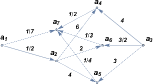
Figure 3: $T_{\text{UP}(C)}$ - the graph of the upper triangle of the PC matrix $C$ which does not contain triads

Since we can not use triads in this case, the question arises as to whether we should not use quadruples $(c_{ik},c_{kr},c_{rj},c_{ij})$ i.e. cycles with the length $4$. As in the previous case, the answer is negative. We are able to construct a directed graph without cycles with the length $4$ and, as follows, a PC matrix which does not contain quadruples. Fortunately, there are some cycles in most strongly connected graphs of the PC matrices. The only exceptions are the strongly connected graphs with $n$ vertices and only $2(n-1)$ edges. In such graphs, every vertex $a_{i}$ is connected with only one other vertex $a_{j}$ by two edges $(a_{i},a_{j})$ and $(a_{j},a_{i})$. If we remove any pair of the existing edges $\{(a_{i},a_{j}),(a_{j},a_{i})\}$, the graph would cease to be strongly connected. Conversely, if we add a new pair of edges $\{(a_{p},a_{q}),(a_{q},a_{p})\}$ to $E$ it would be a cycle in the graph. For this reason, whenever there are cycles in $T_{C}$, we will try to use them all to inconsistency without limiting their length or quantity. However, if there are no cycles in the graph, the concept of inconsistency loses meaning. Therefore, the only option is to accept that the considered PC matrix is consistent (an alternative would be to assume that the inconsistency is indeterminate).

In order to use the cycle to determine the matrix inconsistency, let us extend the Definition 4.

Definition 12.

A PC matrix $C=[c_{ij}]$ is said to be inconsistent if there exists a cycle $a_{i_{1}},\ldots,a_{i_{m}}$ in $T_{C}$ such that $c_{i_{1}i_{2}}c_{i_{2}i_{3}}\cdot\ldots\cdot c_{i_{m-1}i_{m}}\neq c_{i_{1}i_{m}}$. Otherwise $C$ is consistent.

For complete PC matrices, both definitions 4 and 12 are equivalent. To prove that, it is enough to show that wherever $C$ is inconsistent in the sense (Def. 4) then it is also inconsistent in the sense (Def. 12), and reversely inconsistency in the sense (Def. 12) entails inconsistency in the sense (Def. 4).

Theorem 13.

Every complete PC matrix $C$ is inconsistent in the sense of (Def. 4) if and only if it is inconsistent in the sense of (Def. 12)

Proof.

“$\Rightarrow$” Let $C$ be inconsistent in the sense of (Def. 4) i.e. there is a triad such that $c_{ik}c_{kj}\neq c_{ij}$. Since this triad is also a cycle with the length $3$, $C$ is also inconsistent in the sense of (Def. 12).

“$\Leftarrow$” Let $C$ be inconsistent in the sense of (Def. 12) i.e. there is a cycle $s=a_{i_{1}},\ldots,a_{i_{m}}$ such that $c_{i_{1}i_{2}}c_{i_{2}i_{3}}\cdot\ldots\cdot c_{i_{m-1}i_{m}}\neq c_{i_{1}i_{m}}$,

and let us suppose for a moment that $C$ is consistent in the sense of (Def. 4). The latter assumption means that every triad is consistent, thus, in particular it also holds that $c_{i_{1}i_{2}}c_{i_{2}i_{3}}=c_{i_{1}i_{3}}$. Therefore, the first assumption can be written in the form: $c_{i_{1}i_{3}}\cdot\ldots\cdot c_{i_{m-1}i_{m}}\neq c_{i_{1}i_{m}}$. Applying the same reasoning many times, we subsequently get that $c_{i_{1}i_{4}}\cdot\ldots\cdot c_{i_{m-1}i_{m}}\neq c_{i_{1}i_{m}}$, $c_{i_{1}i_{5}}\cdot\ldots\cdot c_{i_{m-1}i_{m}}\neq c_{i_{1}i_{m}}$ and finally $c_{i_{1}i_{m-1}}\cdot c_{i_{m-1}i_{m}}\neq c_{i_{1}i_{m}}$. However, as we assume that every triad is consistent, therefore also $a_{i_{1}},a_{i_{m-1}},a_{m}$ is consistent, thus it must hold that $c_{i_{1}i_{m-1}}\cdot c_{i_{m-1}i_{m}}=c_{i_{1}i_{m}}$. Contradiction. ∎

Of course, when $C$ is incomplete the two above definitions of inconsistency are not equivalent. In particular, there may be PC matrices which do not have any triads, hence they have to be considered as consistent, but the same matrices may have graphs with cycles longer than $4$ that might be inconsistent. In general, however, the cycle based definition of inconsistency is more general than the Def. 4. We may observe the following property.

Remark 14.

Every PC matrix (complete and incomplete) inconsistent in the sense (Def. 4) is also inconsistent in the sense of (Def. 12), but not reversely.

Definition 12 also allows us to quantify the inconsistency. As we will see later on, the ratio:

$$R_{s}\overset{\textit{df}}{=}\frac{c_{i_{1}i_{2}}\cdot\ldots\cdot c_{i_{m-1}i_{m}}}{c_{i_{1}i_{m}}}$$ (25)

defined for a cycle $s=a_{i_{1}},\ldots,a_{i_{m}}$ is a useful way for measuring inconsistency within the set of $m$ alternatives $a_{i_{1}},\ldots,a_{i_{m}}$. We use this fact to define several matrix based indices for an incomplete PC matrix. The idea of using cycles for inconsistency measurement can be found in [5, 33].

4.2 Ranking based indices

The ranking based indices need the results of ranking in order to calculate inconsistency. The considered indices use two different priority deriving methods: EVM (2) and GMM (3). Although both methods have been defined for a complete PC matrix, they have their counterparts for incomplete PC matrices (Section 2.3). These are the HM [28] and ILLS approaches [4].

The starting point of both extensions is the assumption that every missing value $c_{ij}$ in $C$ should eventually take the value $w(a_{i})/w(a_{j})$. Therefore, the authors of extensions replaced the unknown values by the appropriate ratios, and then tried to solve such modified problems. Let $\widehat{C}$ be a PC matrix obtained from $C$ by replacing every $c_{ij}=?$ by $w(a_{i})/w(a_{j})$. In HM, the eigenvalue equation (2) takes the form:

$$\widehat{C}w=\lambda_{\textit{max}}w,$$

and after the appropriate transformations, we finally get

$$Bw=\lambda_{\textit{max}}w$$

where $B$ is an auxiliary matrix (8). Similarly, in the ILLS method [4], the authors define the priority of the i-th alternative as the geometric mean of the i-th row of $\widehat{C}$. The adoption of this assumption leads to the matrix equation (9), whose solution determines the desirable vector of priorities.

In general, the ranking based indices define the inconsistency as the differences between $c_{ij}$ and $w(a_{i})/w(a_{j})$ for $i,j=1,\ldots,n$. Since both HM and ILLS replace every $c_{ij}=?$ by the corresponding ratio $w(a_{i})/w(a_{j})$, then the missing judgments do not contribute to the inconsistency, but are considered as perfectly consistent. From a practical point of view, during construction of the ranking based indices for incomplete PC matrices, we can either ignore the missing values or just assume that $c_{ij}=?$ equals $w(a_{i})/w(a_{j})$.

5 Matrix based indices for incomplete PC matrices

5.1 Koczkodaj index

The Koczkodaj index is directly based on the concept of a triad and its inconsistency. Thus, as explained above (Sec. 4.1), a triad’s inconsistency has to be replaced by the cycle’s inconsistency. Let $C$ be an irreducible and incomplete PC matrix (Def. 5) and $T_{C}$ be a graph of $C$ (Def. 6). Then let us define the inconsistency of a single cycle longer than $2$ i.e. $s\in\mathcal{S}_{C,2}$ as

$$K_{s}\overset{\textit{df}}{=}\min\left\{\left|1-R_{s}\right|,\left|1-R_{s}^{-1}\right|\right\}$$ (26)

Then the Koczkodaj index for the incomplete PC matrix $C$ can be defined as:

$$\widetilde{K}\overset{\textit{df}}{=}\begin{cases}\max\left\{K_{s}:s\in\mathcal{S}_{C,2}\right\}&\left|\mathcal{S}_{C,2}\right|>0\\ 0&\left|\mathcal{S}_{C,2}\right|=0\end{cases}$$

The case in which $\left|\mathcal{S}_{C,2}\right|=0$ refers to the situation when the $n\times n$ matrix $C$ is irreducible, but it contains exactly $n-1$ comparisons i.e. $T_{\textit{UP}(C)}$ is a tree [14].

5.2 Triad based average inconsistency indices

The method of replacing triads with cycles can be successfully used in the case of triad based average inconsistency indices. Thus, providing that $C$ is an irreducible and incomplete PC matrix, we have:

$$\widetilde{I}_{1}\overset{\textit{df}}{=}\begin{cases}\frac{\sum_{s\in\mathcal{S}_{C,2}}K_{s}}{\left|\mathcal{S}_{C,2}\right|}&\left|\mathcal{S}_{C,2}\right|>0\\ 0&\left|\mathcal{S}_{C,2}\right|=0\end{cases},$$

and correspondingly,

$$\widetilde{I}_{2}\overset{\textit{df}}{=}\begin{cases}\frac{\sqrt{\sum_{s\in\mathcal{S}_{C,2}}K_{s}^{2}}}{\left|\mathcal{S}_{C,2}\right|}&\left|\mathcal{S}_{C,2}\right|>0\\ 0&\left|\mathcal{S}_{C,2}\right|=0\end{cases}.$$

The $I_{\alpha}$ and $I_{\alpha,\beta}$ indices (18, 19) also need to be changed accordingly.

$$\widetilde{I}_{\alpha}\overset{\textit{df}}{=}\alpha\widetilde{K}+(1-\alpha)\widetilde{I}_{1},$$

$$\widetilde{I}_{\alpha,\beta}\overset{\textit{df}}{=}\alpha\widetilde{K}+\beta\widetilde{I}_{1}+(1-\alpha-\beta)\widetilde{I}_{2}.$$

5.3 Salo and Hamalainen index

The SHI index is based on the observation that every product $c_{ik}c_{kj}$ for any $k=1,\ldots,n$ is an approximation of $c_{ij}$ [53]. When $C$ is irreducible, due to the strong connectivity of $T_{C}$ between every two vertices $a_{q}$ and $a_{j}$ there is a path $p=a_{q},a_{i_{2}},a_{i_{2}},\ldots,a_{i_{m-1}},a_{j}$ (Def. 9). This means that $c_{q,i_{2}},c_{i_{2}i_{3},}\ldots,c_{i_{m-1},j}$ are defined. Let us denote the product induced by $p$ as $\pi_{p}=c_{q,i_{2}}c_{i_{2}i_{3},}\cdot\ldots\cdot c_{i_{m-1},j}$. Due to (5 - 6), $\pi_{p}$ is also a good approximation of $c_{ij}$. Thus, let us define

$$\underset{\widetilde{\,\,\,\,\,}}{r}{}_{ij}\overset{\textit{df}}{=}\min\left\{\pi_{p}\mid p\in\mathcal{P}_{C,i,j}\right\}$$

and

$$\widetilde{r}_{ij}\overset{\textit{df}}{=}\max\left\{\pi_{p}\mid p\in\mathcal{P}_{C,i,j}\right\}$$

The modified $I_{\textit{SH}}$ index can be defined as

$$\widetilde{I}_{\textit{SH}}\overset{\textit{df}}{=}\frac{2}{n(n-1)}\sum_{i=1}^{n-1}\sum_{j=i+1}^{n}\frac{\widetilde{r}_{ij}-\underset{\widetilde{\,\,\,\,\,}}{r}{}_{ij}}{\left(1+\widetilde{r}_{ij}\right)\left(1+\underset{\widetilde{\,\,\,\,\,}}{r}{}_{ij}\right)}.$$

6 Ranking based indices for incomplete PC matrices

6.1 Geometric consistency index

The geometric consistency index (12) is directly based on observation (5) i.e. $w(a_{i})/w(a_{k})\approx c_{ik}$, where $w$ is the priority vector obtained from GMM [15, 1]. In an incomplete PC matrix, a priority vector $\widetilde{w}$ has to be computed using the ILLS method (Sec. 2.3). Following this method wherever $c_{ij}=?$ it is replaced by $\widetilde{w}(a_{i})/\widetilde{w}(a_{j})$. This leads to the following formula:

$$\widetilde{I}_{G1}\overset{\textit{df}}{=}\frac{2}{(n-1)(n-2)}\sum_{e\in\mathscr{E}}\log^{2}e,$$ (27)

where $C=[c_{ij}]$, $\widetilde{w}=[\widetilde{w}(a_{1}),\ldots,\widetilde{w}(a_{n})]^{T}$ is the ranking vector calculated using the ILLS method, and $\mathscr{E}\overset{\textit{df}}{=}\left\{e_{ij}=c_{ij}\frac{\widetilde{w}(a_{j})}{\widetilde{w}(a_{i})}\,:\,c_{ij}\neq?\,\,\text{and}\,\,i<j\right\}$. The second way to extend the GCI index is to calculate the average of all non-zero $\log^{2}e$ expressions also possible. In this approach we assume that $c_{ij}=?$ does not contribute to our knowledge about inconsistency. Hence, the second version of GCI for incomplete PC matrices is as follows:

$$\widetilde{I}_{G2}\overset{\textit{df}}{=}\frac{1}{\left|\mathscr{E}\right|}\sum_{e\in\mathscr{E}}\log^{2}e.$$

6.2 Golden-Wang index

The Golden-Wang index is based on the observation that every column of a consistent PC matrix equals the ranking vector multiplied by some constant scaling factor [25]. Thus, after scaling every column so that it sums up to $1$, it holds that $c_{ij}^{*}=w(a_{i})$, where $C^{*}=[c_{ij}^{*}]$ is the consistent PC matrix with the rescaled columns. The difference between $c_{ij}^{*}$ and $w(a_{i})$ is higher when the inconsistency is greater.

Despite the fact that the observations remain true for any priority deriving method, the authors recommend using GMM (4). The relationship between $c_{ij}^{*}$ and $w(a_{i})$ also remains valid in the case of an incomplete PC matrix, however, due to the missing values the scaling procedure needs to be modified. Let us consider the k-th column of the irreducible incomplete PC matrix $C$ and the ranking vector $w$. Let every element of $C$ be either $1$ or $?$. So it is easy to see that the ranking vector is composed of the same $1/n$ values. For example, for a $5\times 5$ matrix we may have:

$$\left[\begin{array}[]{c}c_{1k}\\ c_{2k}\\ c_{3k}\\ c_{4k}\\ c_{5k}\end{array}\right]=\left[\begin{array}[]{c}1\\ 1\\ 1\\ ?\\ ?\end{array}\right],\,\,\,\,\left[\begin{array}[]{c}w(a_{1})\\ w(a_{2})\\ w(a_{3})\\ w(a_{4})\\ w(a_{5})\end{array}\right]=\left[\begin{array}[]{c}1/5\\ 1/5\\ 1/5\\ 1/5\\ 1/5\end{array}\right],$$

where $k=1,2$ or $3$. Then, after scaling (so that the sum of elements is one) the k-th column is:

$$\left[\begin{array}[]{c}c_{1k}\\ c_{2k}\\ c_{3k}\\ c_{4k}\\ c_{5k}\end{array}\right]=\left[\begin{array}[]{c}1/3\\ 1/3\\ 1/3\\ ?\\ ?\end{array}\right]$$

as the undefined elements cannot be scaled. It is evident that $c_{ik}^{*}\neq w(a_{i})$ for $i=1,2,3$ as $1/3\neq 1/5$. The solution is to construct the priority vector $w_{k}$ which has the missing values at the same positions as the k-th column. Let us consider:

$$\left[\begin{array}[]{c}c_{1k}\\ c_{2k}\\ c_{3k}\\ c_{4k}\\ c_{5k}\end{array}\right]=\left[\begin{array}[]{c}1\\ 1\\ 1\\ ?\\ ?\end{array}\right],\,\,\,\,\left[\begin{array}[]{c}w_{k}(a_{1})\\ w_{k}(a_{2})\\ w_{k}(a_{3})\\ w_{k}(a_{4})\\ w_{k}(a_{5})\end{array}\right]=\left[\begin{array}[]{c}1/5\\ 1/5\\ 1/5\\ ?\\ ?\end{array}\right]$$

In such a case, after scaling, indeed $c_{ik}^{*}=w_{k}^{*}(a_{i})=1/3$ for $i=1,2,3$.

The above observation shows the way in which the Golden-Wang index can be extended to incomplete pairwise comparisons. Let us define this extension more formally. For this purpose, let us assume that $C$ is an irreducible, incomplete PC matrix, and $w$ is the ranking vector calculated using the ILLS method. Then let $\Omega=[\omega_{ij}]$ be an $n\times n$ matrix such that

$$\omega_{ij}\overset{\textit{df}}{=}\begin{cases}w(a_{i})&\text{if}\,\,c_{ij}\neq?\\ ?&\text{if}\,\,c_{ij}=?\end{cases}.$$

Next, let us scale every column in $\Omega$ and in $C$ so that all the elements in the column sum up to one (in both cases, undefined values are omitted, i.e. only defined elements are subject to scaling). As a result, we get two matrices $C^{*}=[c_{ij}^{*}]$ and $\Omega^{*}=[\omega_{ij}^{*}]$ with the appropriately rescaled columns. The absolute differences between the entries of these two matrices form the Golden-Wang index for incomplete PC matrices. Thus, following (20), we may define:

$$\widetilde{\textit{GW}}\overset{\textit{df}}{=}\frac{1}{n}\sum_{i=1}^{n}\sum_{j=1}^{n}\mid c_{ij}^{*}-\omega_{ij}^{*}\mid$$

6.3 Relative Error

In general, Barzilai’s Relative Error RE has been defined for additive PC matrices [3]. For the purpose of this paper we use its logarithmized version suitable for multiplicative matrices [3]. For an incomplete PC matrix, similarly to the case of the GCI index, we may assume that $w$ is calculated using the ILLS method (for multiplicative matrices Barzilai’s original approach uses GMM). The use of the ILLS method implies the assumption that every $c_{ij}=?$ can be substituted by $w_{\textit{ILLS}}(a_{i})/w_{\textit{ILLS}}(a_{j})$. In particular, in such a case $e_{ij}=0$, hence in the formula (LABEL:eq:relative-error-log-form) they can be omitted. Thus, the relative error for the incomplete multiplicative PC matrix $C$ takes the form:

$$\widetilde{\textit{RE}}_{1}\overset{\textit{df}}{=}\frac{\sum_{c_{ij}\neq?}\left[\log c_{ij}\frac{w_{\textit{ILLS}}(a_{j})}{w_{\textit{ILLS}}(a_{i})}\right]^{2}}{\sum_{c_{ij}\neq?}\log^{2}c_{ij}+\sum_{c_{ij}=?}\log^{2}\frac{w_{\textit{ILLS}}(a_{i})}{w_{\textit{ILLS}}(a_{j})}},$$

where $i,j=1,\ldots,n$. Another way of extending Relative Error to incomplete, multiplicative PC matrices is to skip all the expressions requiring missing comparisons. Similarly to the case of the geometric consistency index, this leads to a shorter formula:

$$\widetilde{\textit{RE}}_{2}\overset{\textit{df}}{=}\frac{\sum_{c_{ij}\neq?}\left[\log c_{ij}\frac{w_{\textit{ILLS}}(a_{j})}{w_{\textit{ILLS}}(a_{i})}\right]^{2}}{\sum_{c_{ij}\neq?}\log^{2}c_{ij}}.$$

7 Numerical experiment

Does increasing incompleteness affect inconsistency? Intuition suggests that it should not. If decision makers responsible for creating PC matrices are inconsistent in their judgments, then we may assume that their inconsistency will not depend on whether they answer all or only part of the questions. The only difference is that in the case of a complete matrix the experts will more often do both: make mistakes and respond correctly. Of course, we implicitly assume that the experts are able to consider each question with similar attention, i.e. questions are not too many, experts have enough time to think about them, and they are professionals in the field. So if indeed inconsistency does not depend on incompleteness, then the incomplete matrix can be treated just as a sample of some complete PC matrix. Of course, there may always be some differences between the sample and the entire population, but it is natural to expect that they are reasonably small.

In light of these observations, it seems interesting to see how much the inconsistency for the complete matrix will differ from its incomplete sample with reference to the given inconsistency index, i.e. how robust the given inconsistency index is for the PC matrix deterioration. To this end, we created $1000$ consistent $7\times 7$ PC matrices. Then, the entries of each matrix were disturbed by multiplying them by the randomly chosen coefficient $\gamma\in[1/d,d]$. We repeated the disturbance procedure $30$ times for $\gamma=1,\ldots,30$. In this way, we received the set $\mathcal{C}$ composed of $30000$ PC matrices with varying degrees of inconsistency.

Every complete $7\times 7$ PC matrix contains $21$ comparisons (entries above the diagonal). On the other hand, the smallest irreducible $7\times 7$ PC matrix has $6$ comparisons (as at least six edges are needed to connect seven different vertices of a graph of a matrix). Hence, preserving irreducibility, at most $15$ comparisons can be safely removed from the complete $7\times 7$ PC matrix. Therefore, for each of the $30000$ complete PC matrices, we prepared 15 randomly incomplete irreducible PC matrices, so that every complete matrix had its “sample” matrix with $1,2$ up to $15$ missing comparisons. Finally, we received $480000$ complete and incomplete PC matrices for which we calculated all $13$ inconsistency indices defined in Sections 5 and 6.

In order to check the robustness of different inconsistency indices, we calculate the directed distance between the inconsistency of the complete matrix and their incomplete counterparts. Let $I(C)-I(C_{k})$ be the ordered distance between where $I(C)$ means the value of the inconsistency index $I$ calculated for a complete matrix $C\in\mathcal{C}$, and $I(C_{k})$ denotes inconsistency of the matrix that was obtained from $C$ by removing $k$ comparisons determined by using $I$. Of course, different indices may take values from various ranges. Therefore, to allow those indices to be compared with each other, the ordered distance is divided by the higher component of each difference. Hence, the rescaled ordered distance $\Delta_{I}(C,C_{k})$ between the inconsistency of two matrices $C$ and $C_{k}$ is given as:

$$\Delta_{I}(C,C_{k})\overset{\textit{df}}{=}\begin{cases}\frac{I(C)-I(C_{k})}{\max\left\{I(C),I(C_{k})\right\}}&\max\left\{I(C),I(C_{k})\right\}>0\\ 0&I(C)=I(C_{k})=0\end{cases}.$$

The above formula also takes into account the situation where $I(C)=I(C_{k})=0$. In such a case, it is assumed that $\Delta(C,C_{k})=0$. The final result is the average ordered distance:

$$D(I,k)\overset{\textit{df}}{=}\frac{1}{\left|\mathcal{C}\right|}\sum_{C\in\mathcal{C}}\Delta_{I}(C,C_{k}).$$ (28)

The subsequent values $D(I,0),D(I,1),\ldots,D(I,15)$ allow the difference between the inconsistency of the complete and incomplete matrix to be assessed with respect to the given index $I$ and the number of missing comparisons $k$.

In an ideal case, $D(I,k)$ should be $0$ for all inconsistency indices and every possible $k$. In practice, of course, it is impossible as not all comparisons in the PC matrix are inconsistent to the same extent. Therefore, it is possible that an incomplete matrix will be less (or more) consistent than its complete counterpart. If the incomplete matrix $C_{k}$ is less inconsistent than the complete matrix $C$, i.e. $I(C)>I(C_{k})$, then $\Delta_{I}(C,C_{k})>0$. Reversely, if the incomplete matrix is more inconsistent than its consistent predecessor, the distance is negative i.e. $\Delta_{I}(C,C_{k})<0.$ In other words, the sign (direction) of a distance $D_{I}$ informs us if there is a greater complete or incomplete PC matrix. The closer $\Delta_{I}(C,C_{k})$ is to $0$, i.e. the smaller $\left|\Delta_{I}(C,C_{k})\right|$ is, the more resistant to incompleteness is the index $I$. For the purpose of this study, a directed distance for all inconsistency indices has been computed using $30000$ matrices, then the results have been averaged as $D(I,k)$. Any particular value of $D(I,k)$ for some fixed $I$ and $k$ can be interpreted as an average value of directed distance for a $7\times 7$ randomly disturbed matrix where $I$ is an inconsistency index, and $k$ is the number of missing elements. Of course: the index is better (more robust) when it is closer to the abscissa. Of course it is possible that for some particular $Q,R,k$ the distance $\left|D(Q,k)\right|$ is greater than $\left|D(R,k)\right|$. However, for $k+1$ it may turn out that $\left|D(Q,k+1)\right|<\left|D(R,k+1)\right|$. In such a case, it is difficult to indicate the winner, as one time $Q$ is better, the other time $R$ is better. Therefore, as the final measure of index robustness, we suggest taking the area between the abscissa and the plot of its rescaled ordered distance (Fig. 4). The discrete counterpart of the size of this area is the sum of the absolute value of subsequent $D(I,k)$ i.e.

$$\mathscr{D}(I)\overset{\textit{df}}{=}\sum_{k=0}^{15}\left|D(I,k)\right|.$$

Of course, the smaller $\mathscr{D}(I)$ the better.

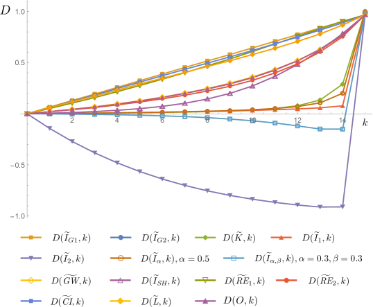
Figure 4: Rescaled ordered distance for different inconsistency indices for incomplete PC matrices with $k$ missing comparisons.

In Figure 4 there are fourteen plots corresponding to the average ordered distance (28) for all the inconsistency indices introduced in 5 and 6 and three additional indices found in the literature. It is easy to see that, in general, the matrix based indices perform better than the ranking based indices. The exception here is the index $\widetilde{I}_{2}$, which very quickly reveals high differences between complete and incomplete PC matrices. It is interesting that the incomplete matrices are considered by this index as more inconsistent than the complete ones (most of the plot is below the abscissa). The behavior of $\widetilde{I}_{2}$ is inherited by the $\widetilde{I}_{\alpha,\beta}$ index. Here, one can also notice that incomplete matrices are considered as more inconsistent than their complete counterparts. Fortunately, the other matrix based indices perform very well. The best of them is $\widetilde{I}_{1}$, where $\mathscr{D}(\widetilde{I}_{1})=1.4256$. Then $\mathscr{D}(\widetilde{I}_{\alpha})=1.5961$, and next $\mathscr{D}(\widetilde{I}_{\alpha,\beta})=1.6882$. Among the ranking based indices, the modification of Salo-Hamalainen index $\widetilde{I}_{\textit{SH}}$ stands out positively as it gets $\mathscr{D}(\widetilde{I}_{\textit{SH}})=4.1286$. The other ranking based indices, like modified Barzilai’s relative error index version 1, get higher areas under the plot. Thus, incompleteness influences the assessment of the degree of inconsistency to a greater extent than for previous indices. All the values of $\mathscr{D}$ are shown in Table 1.

Pos.	Notation	Name	$\mathscr{D}(I)$
$1$.	$\widetilde{I}_{1}$	Cycle based index v. I	$1.3368$
$2$.	$\widetilde{I}_{\alpha}$	$\alpha$-index, for $\alpha=0.5$	$1.5896$
$3$.	$\widetilde{K}$	Koczkodaj index	$1.692$
$4$.	$\widetilde{I}_{\alpha,\beta}$	$\alpha,\beta$-index, for $\alpha=\beta=0.3$	$1.7321$
$5$.	$\widetilde{I}_{\textit{SH}}$	Salo-Hamalainen index	$4.1286$
$6$.	$\widetilde{\textit{RE}}_{2}$	Barzilai’s relative error index v. II	$4.6748$
$7$.	$\widetilde{I}_{G2}$	Geometric consistency index v. II	$4.9048$
$8.$	$O$	Oliva-Setola-Scala’s index	$4.9062$
$9$.	$\widetilde{GW}$	Golden-Wang index	$4.9359$
$10.$	$\widetilde{L}$	Logarithmic least square condition	$7.1425$
$11$.	$\widetilde{\textit{RE}}_{1}$	Barzilai’s relative error index v. I	$7.2958$
$12$.	$\widetilde{\textit{CI}}$	Saaty consistency index	$7.5028$
$13$.	$\widetilde{I}_{G1}$	Geometric consistency index v. I	$7.7333$
$14$.	$\widetilde{I}_{2}$	Cycle based index v. II	$10.112$

Table 1: The total distance $\mathscr{D}$ from the abscissae of the $D(I,k)$ plots for all considered indices. The smaller the value, the more robust the given inconsistency index.

8 Discussion and summary

The four best indices (Table 1) achieve very similar results. They are all very good, which means that the differences in inconsistency measured by these indices between complete and incomplete matrices is small. For instance, $D(\widetilde{I}_{1},4)=0.009$ and $D(\widetilde{I}_{1},11)=0.045$, which means that for $20\%$ of missing comparisons we may expect a difference in value of the index smaller than $1\%$, and for $50\%$ of missing comparisons this difference should not be greater than $4.5\%-5\%$. Such results clearly show that inconsistency measurement for incomplete PC matrices can indeed be a valuable indication of the quality of decision data. Thus, methods for calculating the ranking for incomplete PC matrices mentioned in Section 2.3 also gain methods for estimating data inconsistency.

An obvious disadvantage of the matrix based indices defined in Section 5 is the need to find all cycles in the matrix graph. This can be particularly difficult and time-consuming for larger matrices. A way to deal with a large number of cycles may be to limit their number. This might be achieved by limiting the analysis of inconsistency to fundamental cycles only, or just to a random set of cycles. A similar problem does not occur in the case of the ranking based indices. The best of them, the modification of Salo-Hamalainen index for incomplete PC matrices, gets the total distance $\text{$\mathscr{D}(\widetilde{I}_{\textit{SH}})=$}4.1286$. It is also a good result, which proves that this index can be effectively used to assess the inconsistency of incomplete PC matrices.

The article presents extensions for twelve inconsistency indices that allow them to also be used for incomplete PC matrices. Thanks to this, users of the pairwise comparison method (including AHP) receive a way to determine the quality of incomplete decision data . The presented research does not determine which of the defined indices is the best in practice. Robust indices can be difficult to implement and calculate. On the other hand, indices that are easier to calculate can be more vulnerable for decision data deterioration. Finding a solution that combines robustness with the simplicity of implementation and calculation will still be a challenge for researchers.

Disclosure statement

No potential conflict of interest was reported by the authors.

Funding

The research is supported by The National Science Centre (Narodowe Centrum Nauki), Poland, project no. 2017/25/B/HS4/01617.

Appendix

$k$	$D(\widetilde{I}_{G1},k)$	$D(\widetilde{I}_{G2},k)$	$D(\widetilde{K},k)$	$D(\widetilde{I}_{1},k)$	$D(\widetilde{I}_{2},k)$	$D(\widetilde{I}_{\alpha},k)$	$D(\widetilde{I}_{\alpha,\beta},k)$	$D(\widetilde{GW},k)$	$D(\widetilde{I}_{\textit{SH}},k)$	$D(\widetilde{\textit{RE}}_{1},k)$	$D(\widetilde{\textit{RE}}_{2},k)$	$D(\widetilde{\textit{CI}},k)$	$D(\widetilde{L},k)$	$D(O,k)$
0	0.000	0.000	0.000	0.000	0.000	0.000	0.000	0.000	0.000	0.000	0.000	0.000	0.000	0.000
1	0.065	0.021	0.002	0.002	-0.143	0.002	-0.002	0.021	0.006	0.051	0.019	0.062	0.061	0.020
2	0.129	0.043	0.003	0.004	-0.271	0.004	-0.004	0.043	0.012	0.104	0.039	0.124	0.118	0.042
3	0.192	0.066	0.005	0.006	-0.382	0.006	-0.006	0.068	0.021	0.158	0.060	0.184	0.174	0.065
4	0.258	0.093	0.007	0.009	-0.480	0.009	-0.010	0.096	0.034	0.216	0.087	0.246	0.231	0.094
5	0.323	0.125	0.010	0.012	-0.565	0.012	-0.014	0.127	0.050	0.276	0.115	0.309	0.291	0.125
6	0.388	0.159	0.013	0.015	-0.638	0.016	-0.020	0.162	0.072	0.338	0.146	0.371	0.347	0.160
7	0.452	0.199	0.016	0.019	-0.700	0.020	-0.028	0.201	0.103	0.401	0.181	0.434	0.404	0.200
8	0.516	0.242	0.021	0.023	-0.753	0.025	-0.038	0.246	0.144	0.469	0.222	0.494	0.462	0.243
9	0.579	0.291	0.027	0.027	-0.798	0.031	-0.052	0.298	0.199	0.535	0.269	0.556	0.518	0.294
10	0.643	0.352	0.037	0.033	-0.835	0.039	-0.069	0.358	0.271	0.608	0.326	0.618	0.579	0.353
11	0.708	0.427	0.052	0.040	-0.866	0.051	-0.090	0.431	0.366	0.682	0.399	0.684	0.640	0.429
12	0.773	0.517	0.078	0.047	-0.892	0.070	-0.119	0.519	0.481	0.757	0.488	0.749	0.707	0.518
13	0.838	0.630	0.134	0.058	-0.911	0.106	-0.149	0.627	0.620	0.832	0.604	0.817	0.779	0.628
14	0.902	0.774	0.289	0.077	-0.910	0.200	-0.150	0.766	0.783	0.902	0.754	0.888	0.866	0.768
15	0.967	0.967	1.000	0.967	0.967	0.999	0.981	0.966	0.967	0.967	0.967	0.967	0.967	0.967
	$\mathscr{D}(\widetilde{I}_{G2})$	$\mathscr{D}(\widetilde{I}_{G1})$	$\mathscr{D}(\widetilde{K})$	$\mathscr{D}(\widetilde{I}_{1})$	$\mathscr{D}(\widetilde{I}_{2})$	$\mathscr{D}(\widetilde{I}_{\alpha})$	$\mathscr{D}(\widetilde{I}_{\alpha,\beta})$	$\mathscr{D}(\widetilde{GW})$	$\mathscr{D}(\widetilde{I}_{\textit{SH}})$	$\mathscr{D}(\widetilde{\textit{RE}}_{1})$	$\mathscr{D}(\widetilde{\textit{RE}}_{2})$	$\mathscr{D}(\widetilde{\textit{CI}})$	$\mathscr{D}(\widetilde{L})$	$\mathscr{D}(O)$
	7.733	4.905	1.692	1.337	10.112	1.590	1.732	4.936	4.129	7.296	4.675	7.503	7.143	4.906

References

- [1] J. Aguarón and J. M. Moreno-Jiménez. The geometric consistency index: Approximated thresholds. European Journal of Operational Research, 147(1):137 – 145, 2003.
- [2] K. J. Arrow. A difficulty in the concept of social welfare. The Journal of Political Economy, 1950.
- [3] J. Barzilai. Consistency measures for pairwise comparison matrices. Journal of Multi-Criteria Decision Analysis, 7(3):123–132, 1998.
- [4] S. Bozóki, J. Fülöp, and L. Rónyai. On optimal completion of incomplete pairwise comparison matrices. Mathematical and Computer Modelling, 52(1–2):318 – 333, 2010.
- [5] S. Bozóki and V. Tsyganok. The (logarithmic) least squares optimality of the arithmetic (geometric) mean of weight vectors calculated from all spanning trees for incomplete additive (multiplicative) pairwise comparison matrices. International Journal of General Systems, 48(4):362–381, 2019.
- [6] M. Brunelli. Introduction to the Analytic Hierarchy Process. SpringerBriefs in Operations Research. Springer International Publishing, Cham, 2015.
- [7] M. Brunelli. A technical note on two inconsistency indices for preference relations: A case of functional relation. Information Sciences, 357:1–5, August 2016.
- [8] M. Brunelli. Recent Advances on Inconsistency Indices for Pairwise Comparisons - A Commentary. Fundam. Inform., 144(3-4):321–332, 2016.
- [9] M. Brunelli. A survey of inconsistency indices for pairwise comparisons. International Journal of General Systems, 47(8):751–771, September 2018.
- [10] M. Brunelli, L. Canal, and M. Fedrizzi. Inconsistency indices for pairwise comparison matrices: a numerical study. Annals of Operations Research, 211:493–509, February 2013.
- [11] M. Brunelli, A. Critch, and M. Fedrizzi. A note on the proportionality between some consistency indices in the AHP. Applied Mathematics and Computation, 219(14):7901–7906, March 2013.
- [12] M. Brunelli and M. Fedrizzi. Axiomatic properties of inconsistency indices for pairwise comparisons. Journal of the Operational Research Society, 66(1):1–15, Jan 2015.
- [13] J. M. Colomer. Ramon Llull: from ‘Ars electionis’ to social choice theory. Social Choice and Welfare, 40(2):317–328, October 2011.
- [14] T. H. Cormen, C. E. Leiserson, R. L. Rivest, and C. Stein. Introduction to Algorithms. MIT Press, 3rd edition, 2009.
- [15] G. Crawford and C. Williams. The Analysis of Subjective Judgment Matrices. Technical report, The Rand Corporation, 1985.
- [16] G. B. Crawford. The geometric mean procedure for estimating the scale of a judgement matrix. Mathematical Modelling, 9(3–5):327 – 334, 1987.
- [17] R. Crawford and C. Williams. A note on the analysis of subjective judgement matrices. Journal of Mathematical Psychology, 29:387 – 405, 1985.
- [18] Y. Dong, Y. Xu, H. Li, and M. Dai. A comparative study of the numerical scales and the prioritization methods in AHP. European Journal of Operational Research, 186(1):229–242, March 2008.
- [19] Z. Duszak and W. W. Koczkodaj. Generalization of a new definition of consistency for pairwise comparisons. Information Processing Letters, 52(5):273 – 276, 1994.
- [20] G. T. Fechner. Elemente der Psychophysik. Breitkopf und Härtel, Leipzig, 1860.
- [21] M. Fedrizzi and S. Giove. Incomplete pairwise comparison and consistency optimization. European Journal of Operational Research, 183(1):303–313, 2007.
- [22] M. Fedrizzi and S. Giove. Optimal sequencing in incomplete pairwise comparisons for large-dimensional problems. International Journal of General Systems, 42(4):366–375, February 2013.
- [23] E. H. Forman. Facts and fictions about the analytic hierarchy process. Mathematical and Computer Modelling, 17(4-5):19–26, February 1993.
- [24] J. Franek and A. Kresta. Judgment Scales and Consistency Measure in AHP. Procedia Economics and Finance, 12:164–173, 2014.
- [25] B. L. Golden and Q. Wang. An Alternate Measure of Consistency, pages 68–81. Springer Berlin Heidelberg, Berlin, Heidelberg, 1989.
- [26] A. Z. Grzybowski. New results on inconsistency indices and their relationship with the quality of priority vector estimation. Expert Systems with Applications, 43:197–212, January 2016.
- [27] P. T. Harker. Alternative modes of questioning in the analytic hierarchy process. Mathematical Modelling, 9(3):353 – 360, 1987.
- [28] P. T. Harker. Incomplete pairwise comparisons in the analytic hierarchy process. Mathematical Modelling, 9(11):837–848, 1987.
- [29] W. Ho and X. Ma. The state-of-the-art integrations and applications of the analytic hierarchy process. European Journal of Operational Research, 267:399–414, 2018.
- [30] N. V. Hovanov, J. W. Kolari, and M. V. Sokolov. Deriving weights from general pairwise comparison matrices. Mathematical Social Sciences, 55(2):205 – 220, 2008.
- [31] J. Jablonsky. Analysis of selected prioritization methods in the analytic hierarchy process. Journal of Physics: Conference Series, 622(1):1–7, 2015.
- [32] W. W. Koczkodaj. A new definition of consistency of pairwise comparisons. Math. Comput. Model., 18(7):79–84, October 1993.
- [33] W. W. Koczkodaj and R. Szwarc. On axiomatization of inconsistency indicators in pairwise comparisons. Fundamenta Informaticae, 132(485-500), 2014.
- [34] W. W. Koczkodaj and R. Urban. Axiomatization of inconsistency indicators for pairwise comparisons. International Journal of Approximate Reasoning, 94:18–29, March 2018.
- [35] W.W. Koczkodaj and R. Szwarc. On axiomatization of inconsistency indicators for pairwise comparisons. Fundamenta Informaticae, 4(132):485–500, 2014.
- [36] G. Kou and C. Lin. A cosine maximization method for the priority vector derivation in AHP. European Journal of Operational Research, 235(1):225–232, May 2014.
- [37] K. Kułakowski. On the properties of the priority deriving procedure in the pairwise comparisons method. Fundamenta Informaticae, 139(4):403 – 419, July 2015.
- [38] K. Kułakowski. Notes on the existence of a solution in the pairwise comparisons method using the heuristic rating estimation approach. Annals of Mathematics and Artificial Intelligence, 77(1):105–121, 2016.
- [39] K. Kułakowski. Inconsistency in the ordinal pairwise comparisons method with and without ties. European Journal of Operational Research, 270(1):314 – 327, 2018.
- [40] K. Kułakowski. On the geometric mean method for incomplete pairwise comparisons. CoRR, abs/1905.04609, 2019.
- [41] K. Kułakowski and A. Kedzior. Some Remarks on the Mean-Based Prioritization Methods in AHP. In Ngoc-Thanh Nguyen, Lazaros Iliadis, Yannis Manolopoulos, and Bogdan Trawiński, editors, Lecture Notes In Computer Science, Computational Collective Intelligence: 8th International Conference, ICCCI 2016, Halkidiki, Greece, September 28-30, 2016. Proceedings, Part I, pages 434–443. Springer International Publishing, 2016.
- [42] K. Kułakowski and J. Szybowski. The new triad based inconsistency indices for pairwise comparisons. Procedia Computer Science, 35(0):1132 – 1137, 2014.
- [43] K. Kułakowski, J. Szybowski, and A. Prusak. Towards quantification of incompleteness in the pairwise comparisons methods. International Journal of Approximate Reasoning, 115:221–234, October 2019.
- [44] M. Lundy, S. Siraj, and S. Greco. The mathematical equivalence of the “spanning tree” and row geometric mean preference vectors and its implications for preference analysis. European Journal of Operational Research, pages 1–12, September 2016.
- [45] R. Merris. Laplacian matrices of graphs: a survey. Linear Algebra and its Applications, 197-198:143–176, January 1994.
- [46] C. Meyer. Matrix Analysis and Applied Linear Algebra. SIAM: Society for Industrial and Applied Mathematics, April 2000.
- [47] G. Oliva, R. Setola, and A. Scala. Sparse and distributed Analytic Hierarchy Process. Automatica, 85:211–220, November 2017.
- [48] D. Pan, X. Liu, J. Liu, and Y. Deng. A Ranking Procedure by Incomplete Pairwise Comparisons Using Information Entropy and Dempster-Shafer Evidence Theory. The Scientific World Journal, pages 1–11, August 2014.
- [49] A. Quarteroni, R. Sacco, and F. Saleri. Numerical mathematics. Springer Verlag, 2000.
- [50] T. L. Saaty. A scaling method for priorities in hierarchical structures. Journal of Mathematical Psychology, 15(3):234 – 281, 1977.
- [51] T. L. Saaty. The analytic hierarchy and analytic network processes for the measurement of intangible criteria and for decision-making. In Multiple Criteria Decision Analysis: State of the Art Surveys, volume 78 of International Series in Operations Research and Management Science, pages 345–405. Springer New York, 2005.
- [52] T. L. Saaty and G. Hu. Ranking by eigenvector versus other methods in the analytic hierarchy process. Applied Mathematics Letters, 11(4):121–125, 1998.
- [53] A. A. Salo and R. P. Hämäläinen. Preference programming through approximate ratio comparisons. European Journal of Operational Research, 82(3):458 – 475, 1995.
- [54] Amartya K Sen. Social Choice Theory: A Re-examination. Econometrica, 45(1):53–89, January 1977.
- [55] S. Siraj, L. Mikhailov, and J. A. Keane. Enumerating all spanning trees for pairwise comparisons. Computers and Operations Research, 39(2):191–199, February 2012.
- [56] B. Srdjevic, Z. Srdjevic, and B. Blagojevic. First-Level Transitivity Rule Method for Filling in Incomplete Pair-Wise Comparison Matrices in the Analytic Hierarchy Process. Applied Mathematics & Information Sciences, 8(2):459–467, 2014.
- [57] D. Talaga. Inconsistency of incomplete pairwise comparisons matrices. Master’s thesis, AGH University of Science and Technology, 2018.
- [58] L. L. Thurstone. The Method of Paired Comparisons for Social Values. Journal of Abnormal and Social Psychology, pages 384–400, 1927.
- [59] W. C. Wedley. Consistency prediction for incomplete AHP matrices. Mathematical and Computer Modelling, 17(4-5):151–161, February 1993.
- [60] Y. Wind and T. L. Saaty. Marketing Applications of the Analytic Hierarchy Process. Management Science, 26(7):641–658, 1980.
- [61] K. K. F. Yuen. Compound Linguistic Scale. Applied Soft Computing, 21:38–56, August 2014.