Reversed dynamo at small scales and large magnetic Prandtl number

Abstract

We show that at large magnetic Prandtl numbers, the Lorentz force does work on the flow at small scales and drives fluid motions, whose energy is dissipated viscously. This situation is opposite to that in a normal dynamo, where the flow does work against the Lorentz force. We compute the spectral conversion rates between kinetic and magnetic energies for several magnetic Prandtl numbers and show that normal (forward) dynamo action occurs on large scales over a progressively narrower range of wavenumbers as the magnetic Prandtl number is increased. At higher wavenumbers, reversed dynamo action occurs, i.e., magnetic energy is converted back into kinetic energy at small scales. We demonstrate this in both direct numerical simulations forced by volume stirring and in large eddy simulations of solar convectively driven small-scale dynamos. Low density plasmas such as stellar coronae tend to have large magnetic Prandtl numbers, i.e., the viscosity is large compared with the magnetic diffusivity. The regime in which viscous dissipation dominates over resistive dissipation for large magnetic Prandtl numbers was also previously found in large eddy simulations of the solar corona, i.e., our findings are a more fundamental property of MHD that is not just restricted to dynamos. Viscous energy dissipation is a consequence of positive Lorentz force work, which may partly correspond to particle acceleration in close-to-collisionless plasmas. This is, however, not modeled in the MHD approximation employed. By contrast, resistive energy dissipation on current sheets is expected to be unimportant in stellar coronae.

1. Introduction

The magnetic fields of planets, stars, accretion discs, and galaxies are all produced and maintained by a turbulent dynamo (Zeldovich et al., 1983). Dynamos work through the conversion of kinetic into magnetic energy. This energy conversion is characterized by the flow field doing work against the Lorentz force. It has been known for some time that this energy conversion also depends on the microphysical value of the magnetic Prandtl number, $\mbox{\rm Pr}_{M}\equiv\nu/\eta$, the ratio of kinematic viscosity $\nu$ to magnetic diffusivity $\eta$ (Brandenburg, 2009, 2011). The larger the value of $\mbox{\rm Pr}_{M}$, the larger is also the ratio of kinetic to magnetic energy dissipation (Brandenburg, 2014). This is plausible, because large viscosity means large viscous dissipation ($\epsilon_{\it K}$), and large magnetic diffusivity or resistivity means large resistive dissipation ($\epsilon_{\it M}$). Large values of $\mbox{\rm Pr}_{M}$ are generally expected to occur at low densities, for example in the solar corona ($\mbox{\rm Pr}_{M}\approx 10^{10}$; see Rempel, 2017) and in galaxies ($\mbox{\rm Pr}_{M}\approx 10^{11}$; see Brandenburg and Subramanian, 2005).

In the steady state, $\epsilon_{\it M}$ must be equal to the rate of kinetic to magnetic energy conversion. This becomes clear when looking at an energy flow diagram; see Figure 1(a). It shows that magnetic energy can only be supplied through work done against the Lorentz force, $\mbox{\boldmath$J$}{}\times\bm{B}$, where $\mbox{\boldmath$J$}{}=\mbox{\boldmath$\nabla$}{}\times\bm{B}/\mu_{0}$ is the current density, $\bm{B}$ is the magnetic field, and $\mu_{0}$ is the vacuum permeability. Exactly the same amount of energy must eventually also be dissipated resistively. This implies that at large magnetic Prandtl numbers, not only must most of the energy be dissipated viscously, but also the magnetic energy dissipation must be small. Therefore, also the work done against the Lorentz force must be small, which suggests that the dynamo should be an inefficient one.

A large magnetic Prandtl number implies that the magnetic diffusivity is small, so one would have expected the dynamo to be efficient, because it suffers less dissipation. This immediately leads to a puzzle. How can a dynamo be efficient in the sense of experiencing low energy dissipation, but at the same time inefficient in the sense of having small energy conversion?

Figure 1.— Energy flow diagrams for (a) a standard dynamo and (b) a dynamo at LS with a reversed dynamo at SS. Dashed arrows indicate relatively weak flows of energy.

Here is where our suggestion of a reversed dynamo comes in. A reversed dynamo is one that does work by the Lorentz force—and not against it, as in a usual dynamo. Thus, it corresponds to driving velocity by the Lorentz force and hence to a conversion of magnetic to kinetic energy. Therefore, the idea is that the flow is indeed an inefficient dynamo, but only at large scales (LS), where kinetic energy is converted to magnetic energy. At small scales (SS), however, magnetic energy begins to dominate over kinetic energy, leading therefore to an efficient conversion of magnetic into kinetic energy. This means we have a reversed dynamo, as sketched in Figure 1(b), where we show the flow of energy separately for LS and SS. To test this idea, we analyze solar convection simulations and perform idealized simulations of isotropically forced homogeneous nonhelical turbulence over a range of different magnetic Prandtl numbers and calculate the spectrum of magnetic to kinetic energy transfer.

Mahajan et al. (2005) introduced the concept of a reversed dynamo in the context of large-scale dynamos leading to the formation of large-scale flows that are driven simultaneously with the large-scale field by microscopic fields and flows. In our investigation, we focus on small-scale dynamos and show that small-scale flows are driven by the Lorentz force when $\mbox{\rm Pr}_{M}\gg 1$. The spectral range over which this microscopic reverse dynamo is operational is found to be $\mbox{\rm Pr}_{M}$ dependent and is largest in the high $\mbox{\rm Pr}_{M}$ regimes.

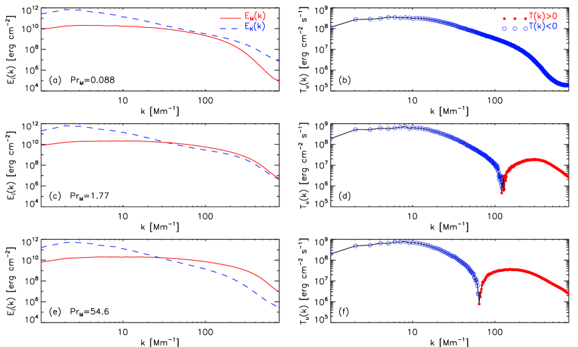
Figure 2.— $E_{i}(k)$ (left) and $T_{u}(k)$ (right) for the LES of Rempel (2018). Open blue (filled red) symbols denote negative (positive) values corresponding to dynamo (reversed dynamo) action. The values of the numerical pseudo $\mbox{\rm Pr}_{M}$ are (a,b) 0.088, (c,d) 1.77, and (e,f) 54.6.

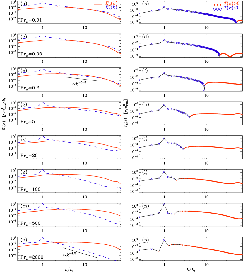
Figure 3.— $E_{i}(k)$ (left) and $T_{u}(k)$ (right) for the DNS of Runs A–H (except Run E’). Open blue (filled red) symbols denote negative (positive) values corresponding to dynamo (reversed dynamo) action. The values of $\mbox{\rm Pr}_{M}$ are (a,b) 0.01, (c,d) 0.05, (e,f) 0.2, (g,h) 5, (i,j) 20, (k,l) 100, (m,n) 500, and (o,p) 2000. The scalings of $k^{-5/3}$ (e) and $k^{-4.2}$ (o) are given for reference.

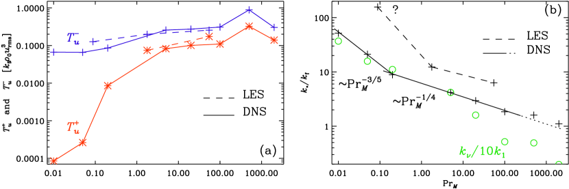
Figure 4.— Dependence of (a) $T_{u}^{\pm}$ and (b) $k_{\ast}$ on $\mbox{\rm Pr}_{M}$ for the DNS (solid lines) and comparison with the LES (dashed lines). In panel (b), the dotted continuation of the solid line indicates the expected breakdown of the $\sim\mbox{\rm Pr}_{M}^{-1/4}$ scaling for $\mbox{\rm Pr}_{M}\mathrel{\mathchoice{\vbox{\offinterlineskip\halign{\hfil$\displaystyle#$\hfil\cr>\cr\sim\cr}}}{\vbox{\offinterlineskip\halign{\hfil$\textstyle#$\hfil\cr>\cr\sim\cr}}}{\vbox{\offinterlineskip\halign{\hfil$\scriptstyle#$\hfil\cr>\cr\sim\cr}}}{\vbox{\offinterlineskip\halign{\hfil$\scriptscriptstyle#$\hfil\cr>\cr\sim\cr}}}}200$. The green open symbols show $k_{\nu}/10k_{1}$ for comparison. The question mark on the leftmost LES data point indicates that $k_{\ast}$ is here only constrained to be $>k_{\rm max}$ for these small values of $\mbox{\rm Pr}_{M}$.

2. Dynamo simulations and analysis

We consider two types of dynamo simulations. On the one hand, we perform direct numerical simulations (DNS; as in Brandenburg, 2014), where viscous and magnetic dissipation are solved for explicitly, and large eddy simulations (LES), where these terms are modeled. In both cases, we vary the ratio of kinetic to magnetic energy dissipation to examine our ideas about reversed dynamo action.

Our main analysis tool is the spectrum of energy conversion, defined as (Rempel, 2014)

$$T_{u}(k)=\Re\!\!\!\!\!\!\!\!\!\sum_{k_{-}<|{\bm{k}}|\leq k_{+}}\!\!\!\!\!\!\!\!\widetilde{\mbox{\boldmath$u$}{}}_{\bm{k}}\cdot\widetilde{(\mbox{\boldmath$J$}{}\times\bm{B})}_{\bm{k}}^{\ast},$$ (1)

where $k_{\pm}=k\pm\delta k/2$, $\delta k=2\pi/L$ is the wavenumber increment and also the smallest wavenumber $k_{1}\equiv\delta k$ in the domain of side length $L$, tildes denote Fourier transformation either in all three directions in the homogeneous DNS or in the two horizontal directions in the inhomogeneous LES, and $\Re$ denotes the real part.

The LES of Rempel (2014, 2018) are designed to model the solar convection zone and use realistic physics such as multifrequency radiation transport and a realistic equation of state allowing for partial ionization effects. Here, the flow is driven by the convection resulting from radiative surface cooling at a rate high enough so that radiative diffusion leads to a superadiabatic stratification, which is Schwarzschild unstable. This model is periodic in the two horizontal directions, but not in the vertical. The employed LES approach allows for different diffusivity settings in the momentum and induction equations resulting in the flexibility to change the effective numerical magnetic Prandtl number; see Equation (10) of Rempel (2014). Beneath the solar photosphere, $\mbox{\rm Pr}_{M}$ is still well below unity, so the purpose of changing its value is solely to demonstrate the effect of such a change on the dynamo in the LES with the MURaM code (Vögler et al., 2005). However, the same code will later also be applied to a model of the solar corona where the actual value of $\mbox{\rm Pr}_{M}$ is much larger than unity. Here, however, we analyze the solar convection setups that were described in Rempel (2018) with effective numerical (or pseudo) $\mbox{\rm Pr}_{M}$ on the order of $0.088$, $1.77$, and $54.6$. It is important to note that the pseudo $\mbox{\rm Pr}_{M}=0.088$ and $1.77$ cases have approximately the same Reynolds number, Re, but different magnetic Reynolds number, $\mbox{\rm Re}_{M}$, whereas the $\mbox{\rm Pr}_{M}=1.77$ and $54.6$ cases have the same $\mbox{\rm Re}_{M}$, but different Re. Note that $\mbox{\rm Pr}_{M}=\mbox{\rm Re}_{M}/\mbox{\rm Re}$.

We should note that, owing to the strong vertical stratification of the density $\rho$ in the LES, we have modified Equation (1) by computing $T_{u}(k)$ with the Fourier transforms as $\overline{\rho}^{1/2}\mbox{\boldmath$u$}{}$ and $\mbox{\boldmath$J$}{}\times\bm{B}/\overline{\rho}^{1/2}$, where overbars denote horizontal averaging. However, the choice of a $\overline{\rho}^{1/2}$ was somewhat arbitrary and one could have used instead $\overline{\rho}^{1/3}$, because $\overline{\rho}(z)\overline{u}_{\rm rms}^{3}(z)$ is known to be an approximation to the convective flux which, in turn, is expected to be approximately constant through the convection zone. Note that the multiplication and division by the same factor does not affect the dimension of $T_{u}(k)$. Incidently, a $\overline{\rho}^{1/3}$ factor has also been advocated by Kritsuk et al. (2007) in the context of supersonic interstellar turbulence. In the present simulations, however, $\overline{\rho}^{1/3}\overline{u}_{\rm rms}$ is seen to increase slightly with height, while $\overline{\rho}^{1/2}\overline{u}_{\rm rms}$ decreases slightly, so the latter choice is equally well justified.

Figure 2 shows the corresponding magnetic and kinetic energy spectra, $E_{\rm M}(k)$ and $E_{\rm K}(k)$, respectively, together with the spectral transfer functions for the three cases with different pseudo $\mbox{\rm Pr}_{M}$. Since the domain is periodic horizontally, but stratified vertically, we consider here only the horizontal Fourier transforms when computing power spectra and transfer functions. In addition, quantities are averaged over a height range of $800$ km ranging from $700$ to $1500$ km beneath the solar photosphere. Unlike the DNS, the LES setup is dimensional, representing a volume of $6.144\times 6.144\times 3.072$ Mm³ in the solar photosphere. Consequently, the LES results presented in the following discussion are dimensional as well.

By contrast, the DNS are statistically fully isotropic and homogeneous, so periodicity is assumed in all three directions and the flow is driven by volume forcing with plane monochromatic nonhelical waves with random phases and wavevectors $\bm{k}(t)$ that are selected randomly at each time step such that $k_{-}<|\bm{k}(t)|\leq k_{+}$ with $k_{\pm}=k_{\rm f}\pm\delta k/2$ and $k_{\rm f}=4\,k_{1}$; see Brandenburg (2001) for details. We use an isothermal equation of state with constant isothermal sound speed $c_{\rm s}$. The typical Mach number based on the rms velocity varies between $u_{\rm rms}/c_{\rm s}\approx 0.056$ for the largest value of $\mbox{\rm Pr}_{M}$ and $0.11$ for the smallest value. We usually vary both $\nu$ and $\eta$ as we change the value of $\mbox{\rm Pr}_{M}$.

Table 1Results from solar LES.

Pseudo $\mbox{\rm Pr}_{M}$ $T_{u}^{+}$ [erg cm^-3 s^-1] $T_{u}^{-}$ [erg cm^-3s^-1] $k_{*}$ [Mm^-1] $\epsilon_{\it K}/\epsilon_{\it M}$ $\overline{\rho}\overline{u}_{\rm rms}^{3}$ ($\langle\rho|\mbox{\boldmath$u$}{}|^{3}\rangle$) $[10^{9}\,{\rm erg}\,{\rm cm}^{-2}\,{\rm s}^{-1}]$ $0.088$ $0$ $152$ $>k_{\rm max}$ $0.27$ $11.5$  ($19.4$) $1.77$ $67$ $179$ $123$ $0.92$ $9.05$  ($15.0$) $54.6$ $104$ $154$ $63$ $4.15$ $5.64$  ($9.06$)

Table 2 Summary of the DNS runs.

Run $\nu k_{1}/c_{\rm s}$ $\eta k_{1}/c_{\rm s}$ Re $\mbox{\rm Re}_{M}$ $\mbox{\rm Pr}_{M}$ $u_{\rm rms}/c_{\rm s}$ $b_{\rm rms}/c_{\rm s}$ $\epsilon_{\it K}/\epsilon_{\it T}$ $\epsilon_{\it M}/\epsilon_{\it T}$ $\epsilon_{\it K}/\epsilon_{\it M}$ $k_{\nu}/k_{1}$ $k_{\eta}/k_{1}$ res. A $1\times 10^{-6}$ $1\times 10^{-4}$ 73000 730 0.01 0.110 0.051 0.01 0.98 0.01 1500 130 $576^{3}$ B $5\times 10^{-6}$ $1\times 10^{-4}$ 15000 730 0.05 0.110 0.051 0.06 0.94 0.07 640 130 $576^{3}$ C $1\times 10^{-5}$ $5\times 10^{-5}$ 6800 1400 0.20 0.102 0.056 0.13 0.87 0.15 450 220 $576^{3}$ D $5\times 10^{-5}$ $1\times 10^{-5}$ 960 4800 5.00 0.072 0.051 0.53 0.47 1.15 170 540 $576^{3}$ E $2\times 10^{-4}$ $1\times 10^{-5}$ 230 4700 20.00 0.070 0.057 0.60 0.40 1.51 65 560 $576^{3}$ E’ $2\times 10^{-3}$ $1\times 10^{-4}$ 27 540 20.00 0.081 0.046 0.70 0.30 2.31 14 110 $576^{3}$ F $1\times 10^{-3}$ $1\times 10^{-5}$ 43 4300 100.00 0.064 0.061 0.65 0.35 1.87 21 560 $576^{3}$ G $1\times 10^{-3}$ $2\times 10^{-6}$ 31 16000 500.00 0.047 0.041 0.81 0.19 4.35 20 1500 $1152^{3}$ H $4\times 10^{-3}$ $2\times 10^{-6}$ 9 19000 2000.00 0.056 0.065 0.85 0.15 5.85 8 1600 $1152^{3}$

In Figure 3, we show $E_{i}(k)$ for $i={\rm K},{\rm M}$ and $T_{u}(k)$ for eight homogeneous DNS at different values of $\mbox{\rm Pr}_{M}$ ranging from $0.01$ to $2000$. We normalize $T_{u}(k)$ by $\rho_{0}u_{\rm rms}^{3}$, where $\rho_{0}$ is the initial (and mean) density and $u_{\rm rms}$ is the root-mean-square (rms) velocity. We clearly see that at small values of $\mbox{\rm Pr}_{M}$, $T_{u}(k)$ is negative at almost all values of $k$, corresponding to work done against the Lorentz work. At larger values of $\mbox{\rm Pr}_{M}$, however, we see a progressively larger span of wavenumbers at small scales, where $T_{u}(k)$ is now positive. This corresponds to reversed dynamo action. Similar results are also seen in the LES presented in Figure 2. For moderate values of $\mbox{\rm Pr}_{M}$, $E_{\rm M}(k)$ and $E_{\rm K}(k)$ show a short range with $k^{-5/3}$ Kolmogorov scalings. For large values of $\mbox{\rm Pr}_{M}$, however, $E_{\rm K}(k)$ has a much steeper spectrum.

As $\mbox{\rm Pr}_{M}$ increases, the areas under the positive and negative parts of $T_{u}(k)$,

$$T_{u}^{+}=\int_{k_{\ast}}^{\infty}T_{u}(k)\,{\rm d}{}k,\quad T_{u}^{-}=-\int_{0}^{k_{\ast}}T_{u}(k)\,{\rm d}{}k,$$ (2)

respectively, become almost equal; see Figure 4(a), where $T_{u}^{\pm}$ is normalized by $k_{\rm f}\rho_{0}u_{\rm rms}^{3}$ for the DNS and by $\langle\overline{\rho}(z)\overline{u}_{\rm rms}(z)^{3}\rangle$ for the LES. However, given that there is always magnetic dissipation at the rate $\epsilon_{\it M}=\langle\eta\mu_{0}\mbox{\boldmath$J$}{}^{2}\rangle$, the difference between $T_{u}^{+}$ and $T_{u}^{-}$ cannot vanish completely, but we have instead $T_{u}^{+}-T_{u}^{-}+\epsilon_{\it M}=0$. (We recall that $T_{u}^{-}>0$ by our definition.) The rest of the energy is dissipated viscously at the rate $\epsilon_{\it K}=\langle 2\rho\nu\mbox{\boldmath${\sf S}$}{}^{2}\rangle$, where ${\sf S}$ is the traceless rate-of-strain tensor; see Brandenburg (2014) for details.

In both the DNS and the LES, we see that the wavenumber $k_{\ast}$, where $T_{u}(k)$ changes sign, moves toward smaller values as $\mbox{\rm Pr}_{M}$ increases. This is shown in Figure 4(b), where $k_{\ast}$ follows an approximate $\mbox{\rm Pr}_{M}^{-1/4}$ scaling for the DNS. For $\mbox{\rm Pr}_{M}\mathrel{\mathchoice{\vbox{\offinterlineskip\halign{\hfil$\displaystyle#$\hfil\cr>\cr\sim\cr}}}{\vbox{\offinterlineskip\halign{\hfil$\textstyle#$\hfil\cr>\cr\sim\cr}}}{\vbox{\offinterlineskip\halign{\hfil$\scriptstyle#$\hfil\cr>\cr\sim\cr}}}{\vbox{\offinterlineskip\halign{\hfil$\scriptscriptstyle#$\hfil\cr>\cr\sim\cr}}}}200$, however, this scaling is seen to level off. This is expected, because in the present case the system also has to sustain a dynamo. For $\mbox{\rm Pr}_{M}<0.1$, however, the scaling is somewhat steeper. Our values of $k_{\ast}$ are typically about ten times smaller than the kinetic energy dissipation wavenumber, $k_{\nu}=(\epsilon_{\it K}/\nu^{3})^{1/4}$, although both quantities scale similarly for $\mbox{\rm Pr}_{M}$ below five; compare with the green open symbols in Figure 4(b). The three data points of $k_{\ast}$ from the LES are also shown in Figure 4(b) and suggest a trend that is compatible with that found in the DNS. As seen from Figure 2(b), in the LES, $T_{u}(k)$ does not change sign for $\mbox{\rm Pr}_{M}<0.1$. We can therefore only assume that $k_{\ast}$ is beyond $k_{\rm max}\approx 800\,{\rm Mm}^{-1}$.

In Table 1 we show the corresponding values of $T_{u}^{+}$ and $T_{u}^{-}$ for the solar LES simulations. Similar to Figure 4(b), we find that $T_{u}^{-}$ only shows a small dependence on $\mbox{\rm Pr}_{M}$, whereas $T_{u}^{+}$ (transfer of inverse dynamo) is increasing with $\mbox{\rm Pr}_{M}$, reducing the net energy transfer $T_{u}^{-}-T_{u}^{+}$ in the high pseudo $\mbox{\rm Pr}_{M}$ case.

It should also be noted that the sign change in the transport term occurs only in the work done against the Lorentz force discussed above. By contrast, magnetic energy must always be gained at all wavenumbers, i.e., in the steady state, the corresponding transport term involving

$$T_{J}(k)=\Re\!\!\!\!\!\!\!\!\!\sum_{k_{-}<|{\bm{k}}|\leq k_{+}}\!\!\!\!\!\!\!\!\widetilde{\mbox{\boldmath$J$}{}}_{\bm{k}}\cdot\widetilde{(\mbox{\boldmath$u$}{}\times\bm{B})}_{\bm{k}}^{\ast}$$ (3)

must always be positive at all wavenumbers so as to balance the resistive losses, which are proportional to $\eta|\widetilde{}\mbox{\boldmath$J$}{}_{k}|^{2}$ and thus positive definite. Looking at Figure 1(b), this simply means that the transfer of magnetic energy from LS to SS must be strong enough to overcome not only the resistive losses, but also those associated with the driving of SS kinetic energy through reversed dynamo action. In this sense, the dynamo must be very efficient at LS.

To compare with the LES results, we normalize them correspondingly. In convection, $\overline{\rho}(z)\overline{u}_{\rm rms}^{3}(z)$ is approximately constant, where $\overline{\rho}(z)$ and $\overline{u}_{\rm rms}(z)$, here with the $z$ argument, indicate horizontally averaged values. It is therefore useful to redefine $\rho_{0}=\langle\overline{\rho}\,\overline{u}_{\rm rms}^{3}\rangle/u_{\rm rms}^{3}$ with $u_{\rm rms}=\langle u_{\rm rms}^{3}(z)\rangle^{1/3}$. From the simulations of Rempel (2014, 2018) we find $\rho_{0}u_{\rm rms}^{3}=(6...12)\times 10^{10}\,{\rm erg}\,{\rm cm}^{-2}\,{\rm s}^{-1}$ for the normalization of the spectral transfer rate adopted in Figure 3. The actual values are listed in Table 1 and compared with the volume average of $\rho|\mbox{\boldmath$u$}{}|^{3}$ over the height range of $800\,{\rm km}$ ranging from $700$ to $1500\,{\rm km}$ beneath the solar photosphere. This volume average turns out to be larger than $\langle\overline{\rho}\,\overline{u}_{\rm rms}^{3}\rangle$ by a factor of between 1.6 (for large $\mbox{\rm Pr}_{M}$) and 1.7 (for small $\mbox{\rm Pr}_{M}$). The value is comparable with the typical values seen in Figure 2. In Figure 4(b), we compare $T_{u}^{\pm}$ from the LES, normalized by $k_{\rm f}\overline{\rho}\,\overline{u}_{\rm rms}^{3}\approx 20\,{\rm erg}\,{\rm cm}^{-3}\,{\rm s}^{-1}$, where we have used for $k_{\rm f}$ the value $10\,{\rm Mm}^{-1}$, which is where $T_{u}(k)$ has a maximum; see Figure 2(b).

Interestingly, $k_{\ast}/k_{\rm f}$ is larger in the LES than in the DNS; see Figure 4(b). This could well be a consequence of not having estimated $k_{\rm f}$ correctly. On the other hand, to achieve better agreement, we would need to use a value of $k_{\rm f}$ that would be even larger than $10\,{\rm Mm}^{-1}$, which is already large compared with the position of the maximum of the magnetic and kinetic energy spectra of around $2.5\,{\rm Mm}^{-1}$. Another difference between LES and DNS is the complete absence of positive values of $T_{u}(k)$ in the low magnetic Prandtl number LES, which was indicated in Table 1 by writing $k_{\ast}>k_{\max}$. This could be a general property of the LES which are very effective in removing power at high wavenumbers, but it could also be an artifact of the DNS being only marginally resolved at large values of $\mbox{\rm Pr}_{M}$. Yet another possibility is that our vertical averaging over different layers may have contributed to washing out the short tail at high wavenumbers. In either case, the trends with $\mbox{\rm Pr}_{M}$ between DNS and LES are clearly the same.

Figure 5.— (a) $E_{\rm K}(k)$ (blue dashed) and $E_{\rm M}(k)$ (red solid lines) showing the saturation of the dynamo at eight different times for Run E’ with $\mbox{\rm Pr}_{M}=20$. (b) The corresponding $T_{u}(k)$, (c) $T_{\rm Str}$, and (d) $T_{\rm Adv}$ with filled red (open blue) symbols denoting positive (negative) values.

3. Caveats

It should be noted that the DNS at extreme magnetic Prandtl numbers are subject to inaccuracies, whose extent cannot be fully quantified as yet. At unit magnetic Prandtl number, the maximum permissible Reynolds number would never be much larger than the number of mesh points, or, more precisely, at least for Kolmogorov-type turbulence, the dissipation wavenumbers for kinetic and magnetic energy dissipation, $k_{\nu}=(\epsilon_{\it K}/\nu^{3})^{1/4}$ and $k_{\eta}=(\epsilon_{\it M}/\eta^{3})^{1/4}$, respectively, should not exceed the Nyquist wavenumber of the mesh, $k_{\rm Ny}=\pi/\delta x$. For $\nu/\eta\gg 1$, we have $k_{\eta}\gg k_{\nu}$, and conversely for $\nu/\eta\ll 1$ we have $k_{\eta}\ll k_{\nu}$. Thus, the larger of the two wavenumbers can severely restrict the simulation and make it numerically unstable. The values of $k_{\nu}$ and $k_{\eta}$ are listed in Table LABEL:Tsummary for Runs A–H.

In the nonlinear regime, however, the rates of energy dissipation are strongly reduced for the longer of the two spectra, because most of the energy is dissipated through the shorter of the two spectra; see the red solid line for $E_{\rm M}(k)$ in Figure 3(a) for $\mbox{\rm Pr}_{M}=0.01$ and the blue dashed line in Figure 3(o) for $\mbox{\rm Pr}_{M}=2000$. This was originally discussed in the context of small $\mbox{\rm Pr}_{M}$, where one also has a constraint on the magnetic Reynolds number, which must be large enough for dynamo action (Brandenburg, 2009, 2011). The simulation may then well be stable even for rather extreme magnetic Prandtl numbers. To what extent we can trust such simulations is unknown, but the similarity with the LES results of Rempel (2014, 2018) suggests that the opposite signs of the energy conversion spectrum and LS and SS, as well as the change of the break point $k_{\ast}$ with $\mbox{\rm Pr}_{M}$ may well be robust. However, there can be other aspects such as the total energy conversion rate, which may not be accurate.

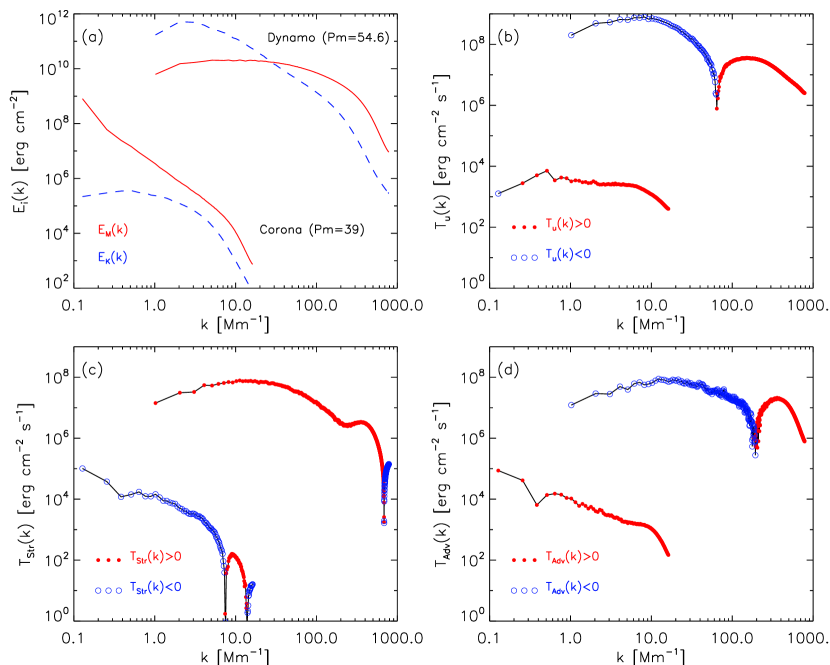
Figure 6.— (a) $E_{\rm K}(k)$ (blue dashed) and $E_{\rm M}(k)$ (red solid lines) for a high $\mbox{\rm Pr}_{M}$ dynamo and corona setup. (b) The corresponding $T_{u}(k)$, (c) $T_{\rm Str}$, and (d) $T_{\rm Adv}$ with filled red (open blue) symbols denoting positive (negative) values.

4. Reversed dynamo prior to saturation

In the kinematic phase of a dynamo, the magnetic field is too weak to drive fluid motions. Conversely, the field cannot resist the fluid motions. To investigate this in more detail, we consider a simulation of a kinematic dynamo at $\mbox{\rm Pr}_{M}=20$. However, as explained above, in the kinematic phase it is not safe to work with Reynolds numbers that are so large that neither $k_{\nu}$ nor $k_{\eta}$ exceed the Nyquist wavenumber $k_{\rm Ny}$. We have therefore computed the kinematic phase for a model with $\mbox{\rm Re}=27$ and $\mbox{\rm Re}_{M}=540$, where $k_{\nu}=14$ or $k_{\eta}=110$ are well below $k_{\rm Ny}/k_{1}=256$. The resulting energy spectra are shown in Figure 5(a).

We see that even in this kinematic case, the same trend of reversed dynamo action occurs in that $T_{u}(k)$ is positive at small scales; see Figure 5(b). This is interesting, because Rempel (2014) found negative values for his kinematic pseudo $\mbox{\rm Pr}_{M}\sim 1$ simulations; see the green dashed lines in his Figure 15(a). This suggests that in his LES, no reversed dynamo action is possible in the kinematic regime at $\mbox{\rm Pr}_{M}\sim 1$. Thus, the exact location of $k_{\ast}/k_{\rm f}$ may also be affected by the absolute value of the fluid Reynolds number, which is not very big in our Run E’, where also $\mbox{\rm Pr}_{M}$ is not unity. However, as the magnetic field in Run E’ saturates, the value of $k_{\ast}/k_{\rm f}$ decreases from about 5 to 2. This suggests that saturation of the dynamo is accomplished, at least partly, by increasing the wavenumber range where reversed dynamo action occurs. At higher wavenumbers, $30<k/k_{\rm f}<50$, there is a persistent range where $T_{u}(k)$ is negative, which was not seen at larger Reynolds numbers. It should be noted, however, that Figure 3(d) gave a hint that a sign reversal in a similar wavenumber range may be possible for slightly different parameters.

The sign reversal of $T_{u}(k)$ suggests that in the subrange $30<k/k_{\rm f}<50$, magnetic energy is no longer fully sustained by the forward cascade of magnetic energy and that it must partially by supported by forward dynamo action just before entering the resistive subrange. In the context of the kinetic energy spectrum in hydrodynamic turbulence, there is a reminiscent feature known as the bottleneck, which is caused by a sufficiently abrupt end of the inertial range (Falkovich, 1994). Whether or not such an analogy is here indeed meaningful can hopefully be decided in future by appropriate analytic studies.

In Figures 5(c) and (d) we show the contributions to $T_{J}(k)$ from stretching and advection: $T_{J}(k)=T_{\rm Str}(k)+T_{\rm Adv}(k)$. We follow here the convention of Rempel (2014) and define

$$T_{\rm Str}(k) =\Re \!\!\!\!\!\!\!\!\!\sum_{k_{-}<|{\bm{k}}|\leq k_{+}}\!\!\!\!\!\!\!\!\!\widetilde{\bm{B}}_{\bm{k}}\!\cdot\!\left[\widetilde{+(\bm{B}\cdot\mbox{\boldmath$\nabla$}{}\mbox{\boldmath$u$}{})}_{\bm{k}}^{\ast}-{\textstyle{1\over 2}}\widetilde{(\bm{B}\mbox{\boldmath$\nabla$}{}\cdot\mbox{\boldmath$u$}{})}_{\bm{k}}^{\ast}\right]\!\!,\;$$ (4)

$$T_{\rm Adv}(k) =\Re \!\!\!\!\!\!\!\!\!\sum_{k_{-}<|{\bm{k}}|\leq k_{+}}\!\!\!\!\!\!\!\!\!\widetilde{\bm{B}}_{\bm{k}}\!\cdot\!\left[\widetilde{-(\mbox{\boldmath$u$}{}\cdot\mbox{\boldmath$\nabla$}{}\bm{B})}_{\bm{k}}^{\ast}-{\textstyle{1\over 2}}\widetilde{(\bm{B}\mbox{\boldmath$\nabla$}{}\cdot\mbox{\boldmath$u$}{})}_{\bm{k}}^{\ast}\right]\!\!.\;$$ (5)

An important reason for including one half of the compression term, $\bm{B}\mbox{\boldmath$\nabla$}{}\cdot\mbox{\boldmath$u$}{}$, in both the stretching and advection terms is that the energy contribution from the latter is a divergence term that vanishes for periodic boundary conditions under volume averaging, that is, $\int T_{\rm Adv}(k)\,{\rm d}{}k=0$. The energy contribution from the former also contains a divergence term, which vanishes for periodic boundaries, while the remaining contribution equals the work against the Lorentz force; see Equations (23) and (24) of Rempel (2014). Therefore, for our DNS with triply periodic boundaries, we have $\int T_{\rm Str}(k)\,{\rm d}{}k=\int T_{u}(k)\,{\rm d}{}k$.

Looking at Figures 5(c) and (d), we see that $T_{\rm Str}(k)$ is positive for all $k$ and $T_{\rm Adv}(k)$ is negative at small $k$ and positive at large $k$. This agrees with the results of Rempel (2014), who interpreted the negative (positive) sign of $T_{\rm Adv}(k)$ at small (large) $k$ as evidence for a transport of magnetic energy from LS (where it acts as a loss) to SS (where it acts as a source). This corresponds to the lower arrow between “magnetic LS” and “magnetic SS” in Figure 1(b). Note that the break point, where $T_{\rm Adv}(k)$ changes sign, does not change much as the dynamo saturates.

5. Applications to stellar coronae

The reversed dynamo phenomenon is a property of large $\mbox{\rm Pr}_{M}$. Since $\mbox{\rm Pr}_{M}\propto T^{4}/\rho$ (e.g., Brandenburg and Subramanian, 2005), where $T$ is the temperature, large $\mbox{\rm Pr}_{M}$ tend to occur in stellar coronae and in galaxies where $\rho$ is very small. Although dynamo action is always possible when $\mbox{\rm Re}_{M}$ is large, it can only occur at LS, that is, for $k<k_{\ast}$, because at SS, or for $k>k_{\ast}$, reversed dynamo action prevails. This implies that most of the magnetic energy will be returned into kinetic energy and then dissipated viscously.

It is not necessarily the case that stellar coronae are dynamos since they are primarily driven through magnetic stresses that build up in response to photospheric footpoint motions, i.e., the energy is injected into the magnetic energy reservoir and does not require a conversion from kinetic energy through a dynamo process. This difference is highlighted in Figure 6 where we present quantities similar to those in Figure 5 for the LES dynamo setup with $\mbox{\rm Pr}_{M}=54.6$ and a corona setup from Rempel (2017) with $\mbox{\rm Pr}_{M}=39$. The corona is evaluated in the height range of $12-24.8$ Mm above the photosphere. In the dynamo case, $T_{\rm Str}$ is positive on almost all scales. $T_{\rm Adv}$ is negative on large and positive on small scales, implying a transport of the magnetic energy induced by $T_{\rm Str}$ to small scales, where it is dissipated most effectively. In the corona case, $T_{\rm Adv}$ is positive on all scales since the corona is driven through the Poynting flux generated by magnetoconvection in the photosphere. $T_{\rm Adv}$ is balanced by a mostly negative $T_{\rm Str}$ (no dynamo). The energy is transferred to kinetic energy through a $T_{u}$, which is positive on all scales, except for the smallest wavenumber. While the dynamo case does have the requirement $T_{u}^{-}>T_{u}^{+}$, this is not the case for the externally driven corona. The scaling shown in Figure 4(b) is then no longer valid. Indeed, coronal transfer functions for smaller $\mbox{\rm Pr}_{M}$ look qualitatively similar to the high $\mbox{\rm Pr}_{M}$ case presented here, i.e., we do not find the $\mbox{\rm Pr}_{M}$ dependence of $k_{*}$ in this study. However, in a corona setup with a 4 times larger domain, we found on large scales a more extended region with $T_{u}<0$. In spite of the significant differences in the underlying transfers, Rempel (2017) found that even for the corona, $\mbox{\rm Pr}_{M}$ determines the value of the ratio $\epsilon_{\it K}/\epsilon_{\it M}$, with dominance of viscous dissipation in the high $\mbox{\rm Pr}_{M}$ regime. Specifically, the simulations of Rempel (2017) that use the coronal arcade setup have $\epsilon_{\it K}/\epsilon_{\it M}$ ratios of $0.23$, $0.83$, and $6.6$ for $\mbox{\rm Pr}_{M}=0.23$, $2.3$, and $39$, respectively (averaged over the height range of $12-24.8$ Mm above the photosphere). The transfer functions for the latter case are presented in Figure 6.

It appears that the dependence of $\epsilon_{\it K}/\epsilon_{\it M}$ on $\mbox{\rm Pr}_{M}$ is a more fundamental property of MHD, whereas the $\mbox{\rm Pr}_{M}$ dependence of $k_{*}$ is specific to dynamo setups that do have, in addition, the constraint $T_{u}^{-}>T_{u}^{+}$. Furthermore, low density plasmas with large values of $\mbox{\rm Pr}_{M}$ are only weakly collisional, and therefore departures from Maxwellian particle velocity distributions and other kinetic effects are expected to play a role (Schekochihin et al., 2009). Much of the kinetic energy may therefore go directly into particle acceleration.

6. Conclusions

Our work has highlighted a qualitatively new feature of dynamos at large magnetic Prandtl numbers, namely the conversion of magnetic energy back into kinetic energy at high wavenumbers or SS. This corresponds to reversed dynamo action. It is responsible for the dissipation of energy through viscous heating rather than through very narrow current sheets that are traditionally thought to be responsible for energy dissipation in the corona (Mikic et al., 1988; Galsgaard & Nordlund, 1996). Current sheets do also occur in large magnetic Prandtl number simulations, but they are not directly responsible for dissipating significant amounts of energy. Instead, viscous energy dissipation is found to be the main mechanism for liberating energy. Viscous energy dissipation is a consequence of positive Lorentz force work, which does occur in proximity of current sheets. While the resulting plasma flows can transport kinetic energy away from current sheets, the resulting viscous dissipation may still happen in close proximity of current sheets, in particular when $\mbox{\rm Pr}_{M}$ is large, and could therefore remain indirectly connected with them.

In kinetic simulations such as those of Rincon et al. (2016) and Zhdankin et al. (2017), reversed dynamo action may be chiefly responsible for particle acceleration. Indeed, the same work term that leads to the conversion of magnetic into kinetic energy also characterizes first-order acceleration of non-thermal particles by curvature drift (Beresnyak & Li, 2016). It will therefore be important to verify this aspect of particle energization in future studies using kinetic simulations. A direct comparison with our work is hampered by the fact that the concept of a magnetic Prandtl number does not exist in collisionless plasmas. A natural question would then be, whether $T^{4}/\rho$ can be regarded as its proxy, as one would expect if Spitzer theory were applicable.

References

- Beresnyak & Li (2016) Beresnyak, A., & Li, H. 2016, ApJ, 819, 90
- Brandenburg (2001) Brandenburg, A. 2001, ApJ, 550, 824
- Brandenburg (2009) Brandenburg, A. 2009, ApJ, 697, 1206
- Brandenburg (2011) Brandenburg, A. 2011, ApJ, 741, 92
- Brandenburg (2014) Brandenburg, A. 2014, ApJ, 791, 12
- Brandenburg and Subramanian (2005) Brandenburg, A., & Subramanian, K. 2005, Phys. Rep., 417, 1
- Falkovich (1994) Falkovich, G. 1994, Phys. Fluids, 6, 1411
- Galsgaard & Nordlund (1996) Galsgaard, K., & Nordlund, Å. 1996, J. Geophys. Res., 101, 13445
- Kritsuk et al. (2007) Kritsuk, A. G., Norman, M. L., Padoan, P., & Wagner, R. 2007, ApJ, 665, 416
- Mahajan et al. (2005) Mahajan, S. M., Shatashvili, N. L., Mikeladze, S. V., & Sigua, K. I. 2005, ApJ, 634, 419
- Mikic et al. (1988) Mikic, Z., Barnes, D. C., & Schnack, D. D. 1988, ApJ, 328, 830
- Rempel (2014) Rempel, M. 2014, ApJ, 789, 132
- Rempel (2017) Rempel, M. 2017, ApJ, 834, 10
- Rempel (2018) Rempel, M. 2018, ApJ, 859, 161
- Rincon et al. (2016) Rincon, F., Califano, F., Schekochihin, A. A., & Valentini, F. 2016, Proc. Nat. Acad. Sci., 113, 3950
- Schekochihin et al. (2009) Schekochihin, A. A., Cowley, S. C., Dorland, W., Hammett, G. W., Howes, G. G., Quataert, E., & Tatsuno, T. 2009, ApJS, 182, 310
- Vögler et al. (2005) Vögler, A., Shelyag, S., Schüssler, M., Cattaneo, F., Emonet, T., & Linde, T. 2005, A&A, 429, 335
- Zeldovich et al. (1983) Zeldovich, Ya. B., Ruzmaikin, A. A., & Sokoloff, D. D. 1983, Magnetic fields in astrophysics (Gordon & Breach, New York)
- Zhdankin et al. (2017) Zhdankin, V., Werner, G. R., Uzdensky, D. A., & Begelman, M. C. 2017, Phys. Rev. Lett., 118, 055103