New phase-magnitude curves for some Main Belt asteroids, fit of different photometric systems and calibration of the albedo - photometry relation

Abstract

Results of photometric observations of a small sample of selected Main Belt asteroids are presented. The obtained measurements can be used to achieve a better calibration of the asteroid photometric system ($H$, $G_{1}$, $G_{2}$) adopted by the IAU, and to make comparisons with best-fit curves that can be obtained using different photometric systems. The new data have been obtained as a first feasibility study of a more extensive project planned for the future, aimed at obtaining a reliable calibration of possible relations between some parameters characterizing the phase-magnitude curves and the geometric albedo of asteroids. This has important potential applications to the analysis of asteroid photometric data obtained by the Gaia space mission.

1 Introduction

The phase - magnitude curve (hereinafter, phase - mag curve) of an asteroid describes the variation of brightness, expressed in magnitudes and normalized to unit distance from Sun and observer, as a function of varying phase angle. The latter is the angle between the directions to the observer and to the Sun as seen from the observed body.

It is well known that the magnitude (by definition, the brightness expressed in a logarithmic scale) of small bodies of the Solar system tends to increase nearly linearly (the objects becoming much fainter) for increasing phase angle. In most cases, a so-called opposition effect is also observed, namely a non-linear magnitude surge occurring when the object is seen close to solar opposition, at phase angles generally below $6^{\circ}$.

The photometric behaviour of atmosphereless Solar system bodies is determined by their macroscopic shapes and by the light scattering properties of their surfaces, related to composition, texture and roughness. In particular, macroscopic roughness and local topographic features of the surface produce shadowing effects, depending upon illumination conditions. Shadows tend to disappear when the object is viewed from nearly the same direction as the illumination, as an object approaches solar opposition. Shadowing effects contribute therefore to the existence of the above-mentioned opposition effect.

It has been known since several decades, however, that another mechanism, named coherent backscattering, plays a more fundamental role in determining the opposition effect. Coherent backscattering is a phenomenon of constructive interference of light beams following different optical paths to reach the observer. It starts to be particularly effective when the body is seen close to solar opposition. Coherent backscattering is enhanced by multiple light scattering, and for this reason it tends to be stronger for asteroids having higher albedo (Muinonen, 1994; Muinonen et al., 2012; Dlugach and Mishchenko, 2013).

Surface scattering properties are responsible not only for the variations of brightness that are measured at different epochs and in different illumination conditions, but also of some corresponding variations in the state of linear polarization of the sunlight scattered by the surfaces. For this reason, the phase - mag curves of asteroids and the corresponding phase - linear polarization curves are fundamental sources of information that in principle can be used to infer hints about important surface properties, including the geometric albedo, the texture and roughness of the regolith, whose determination is in general difficult by using remote observation techniques (Cellino et al., 2016).

So far, however, the number of asteroids for which we have both good-quality phase - mag and phase - polarization curves, is surprisingly limited. This means that it is desirable to set up observing programs aimed at obtaining new phase - mag and phase - polarization curves of the same targets.

On the side of photometry, a most notable effort has been carried out by Shevchenko et al. (2016). The present paper presents the results of a pilot program originally conceived as a feasibility check of a larger project to be carried out at OAVdA (Astronomical Observatory of the Autonomous Region of Aosta Valley). After the end of this program, we were forced to interrupt our photometric activities due to insufficient staffing. In turn, this was also the consequence of a big effort carried out by OAVdA in order to put into operation an array of five new 40-cm telescopes necessary to participate in an European APACHE (A PAthway toward the Characterization of Habitable Earths) project designed for the purpose of the discovery of extrasolar planets, by means of the detection of photometric transit events. Now, after the end of this program in late 2017, we are discussing the possibility to use these APACHE telescopes for the purposes of a new asteroid photometric program aimed at greatly extending the work described in the present paper.

An immediate purpose of our observations was to obtain new asteroid lightcurves to be used to increase the KAMPR database, namely the Kharkiv Asteroid Magnitude-Phase Relations, a list of asteroid phase - mag relations compiled at the Institute of Astronomy of Kharkiv Kharazin University (Shevchenko et al., 2010). At the same time, we wanted to derive for our targets the photometric parameters ($H$, $G_{1}$, $G_{2}$) (Muinonen et al., 2010) using the photometric system adopted at the 2012 IAU General Assembly. In principle, adding new phase - magnitude data is useful to improve the $(H,G_{1},G_{2})$ system, in particular it helps to better determine the values of its base functions. Moreover, we wanted to compare the rms of the computed best-fit curves with those obtained using some other photometric systems still adopted by many authors.

2 The importance of phase - mag curves in the Gaia era

Good-quality phase - mag curves are fundamental to determine asteroid absolute magnitudes. This can be an important information to complement the data produced by the Gaia space mission of the ESA. Gaia is currently collecting a huge data-base of sparse photometric measurements for tens of thousands Main Belt asteroids. Unfortunately, the spacecraft cannot observe these objects when they are seen at phase angles smaller than about $10^{\circ}$ (Gaia Collaboration, 2018). As a consequence, any analysis of the opposition brightness surge is beyond the capability of Gaia, and the photometric data collected by the spacecraft cannot be used in principle to obtain accurate absolute magnitudes of the asteroids.

This is unfortunate, because a fundamental relation links the absolute magnitude to the effective diameter $D_{e}$, and the geometric albedo (Harris and Harris, 1997):

$$D_{e}=\frac{1329}{\sqrt{p}_{V}}10^{-0.2H_{V}}$$ (1)

where $H$ represents the absolute magnitude and $p_{V}$ the geometric albedo. The latter is another key parameter, whose value is determined by composition and texture of the surface regolith.

Gaia has not been designed to have the possibility to determine the albedo of the tens of thousands asteroids that it observes in a variety of observing circumstances, down to a nominal magnitude limit of $20.7$. On the other hand, Gaia can derive phase - mag data taken in an interval of phase angles where the relation between the two parameters is mostly linear.

Interestingly, it has been proposed that the value of such linear slope can be diagnostic of the geometric albedo (Belskaya & Shevchenko, 2000; Shevchenko et al., 2016). This proposed relation deserves confirmation and better calibration, because it opens the possibility to use the phase - mag curves observed by Gaia to infer the corresponding geometric albedo values for tens of thousands asteroids. For this reason, it is important to obtain new good-quality phase-mag curves of asteroids for which the size is known with sufficiently good accuracy, in order to determine for them the absolute magnitude and use Eqn.  1 to derive the corresponding albedo, to be used to calibrate the Belskaya & Shevchenko (2000) relation.

The determination of the absolute magnitudes of the asteroids is not a trivial affair. Due to the non-coplanarity of their orbits with that of the Earth, the objects cannot be seen, as a rule, at ideal Sun opposition, but at a minimum value of phase angle that changes in different apparitions of the same object. As a consequence, the determination of the absolute magnitude is difficult, because the existence of the non-linear brightness opposition effect makes it difficult to extrapolate the observed magnitudes to zero phase angle. In other words, even small differences in the treatment of the opposition effect may lead to important differences in the determination of the absolute magnitude.

In addition, we should not forget that the absolute magnitude, based on its definition, is not, strictly speaking, a really constant parameter, but we can expect it to vary at different apparitions, due to the changing cross section of an object having non-spherical shape when seen in different geometric configurations. In this respect, obtaining the absolute magnitude in different oppositions of the same object can help to improve the estimates of its shape, and the accuracy of the albedo estimates based on thermal radiometry data alone, in the absence of any simultaneous measurements of the visible flux.

According to the above considerations, a systematic program of photometric observations of asteroids to obtain sets of lightcurves obtained at different phase angles is an important task that deserves an investment of time and resources, and can represent a fruitful use of telescopes of even modest aperture. The results of an extensive investigation of the properties of the phase - mag curves of asteroids belonging to different taxonomic classes have been presented by Shevchenko et al. (2016). The observations that we present in this paper for a few objects are nothing but a first pilot program aimed at laying the foundations of a more ambitious long-term project to complement and extend the results obtained by the above authors. At the same time, we consider in our analysis different possible sources of albedo values, from thermal radiometry and from polarimetry, and we consider possible relations between the albedo and a variety of parameters characterising different asteroid photometric systems.

3 Choice of the targets

The observations presented in this paper have been the Master thesis subject of one of us (SC), and were done using the 81-cm reflector telescope of the OAVdA, located in north-western Italian Alps (Calcidese et al., 2012). We selected a limited sample of possible targets, focusing on objects exhibiting apparent magnitudes suitable for the OAVdA telescope, and having sizes well constrained, based on accurate determinations by means of star occultation measurements or reliable thermal infrared data (Masiero et al., 2011), as well as reliable determinations of the geometric albedo, based whenever possible upon polarimetric data (Cellino et al., 2015, 2016) or other data sources (Shevchenko & Tedesco, 2006).

In choosing our targets, we had some obvious constraints related to the epoch of the solar opposition, to be between September and December 2012 on the basis of the interval of time allocated to the project. We made our target selection choosing among objects for which the rotation period is known, and listed in the Asteroid Light Curve Data Base by Warner et al. (2009). We preferentially chose objects having a (moderately) fast rotation, preferred for an easier and faster determination of the lightcurve. Another constraint was the minimum phase angle expected during our observing window. We chose our targets among the objects reaching phase angles around $2^{\circ}$. Unfortunately, weather conditions did not allow us to reach such limit for all the targets of our selected sample. On the other hand, minimum phase angles slightly larger than $5^{\circ}$ could still be useful for the study of the linear part of the phase curve.

We assigned higher priority to targets for which there is a reasonably reliable determination of the geometric albedo, determined using the $\Psi$ polarimetric parameter defined by Cellino et al. (2015) or, when not available, taken from Shevchenko & Tedesco (2006). For all of them, an independent albedo estimate based on thermal radiometry observations by the WISE satelllite, was also available (Masiero et al., 2011).

The list of our targets is shown in Table 1. The Table lists eleven objects, but, as we will see below, could derived good-quality estimates of the absolute magnitude for only six of them.

Table 1: The observed asteroids with rotation periods, geometric albedos, opposition date, minimum phase angle and number of lightcurves. The geometric albedo corresponds to an updated and still unpublished determination of the polarimetric $\Psi$ parameter (as explained in Cellino et al. (2015)). In the case of asteroids (208), (306), (522) and (925), for which no reliable determination of $\Psi$ or other polarimetric parameters is available, we list albedo values taken from (Shevchenko & Tedesco, 2006). The last column gives the number $N$ of different lightcurves obtained for each target. Note that, due to reasons explained in the text, not all the objects listed in this table were eventually used in our analysis of the phase - magnitude curve.

Asteroid	Rotation period (h)	$p_{v}$	Opp. Date	$\alpha_{min}^{\circ}$	$N$
085 Io	6.875	$0.07\pm 0.01$	2012-10-11	0.9	8
135 Herta	8.403	$0.13\pm 0.01$	2012-12-10	1.5	3
208 Lacrimosa	14.085	$0.21\pm 0.02$	2012-11-11	0.7	8
236 Honoria	12.333	$0.19\pm 0.01$	2012-09-21	0.9	9
306 Unitas	8.736	$0.17\pm 0.03$	2012-11-11	5.2	7
308 Polyxo	12.032	$0.10\pm 0.01$	2012-12-17	2.3	5
313 Chaldaea	8.392	$0.07\pm 0.01$	2012-09-22	0.3	6
338 Budrosa	4.608	$0.12\pm 0.01$	2012-12-11	1.5	6
444 Gyptis	6.214	$0.09\pm 0.01$	2013-01-03	5.3	7
522 Helga	8.129	$0.06\pm 0.01$	2012-10-02	1.8	7
925 Alphonsina	7.880	$0.22\pm 0.03$	2012-12-29	5.4	6

4 Instrument and reduction procedures

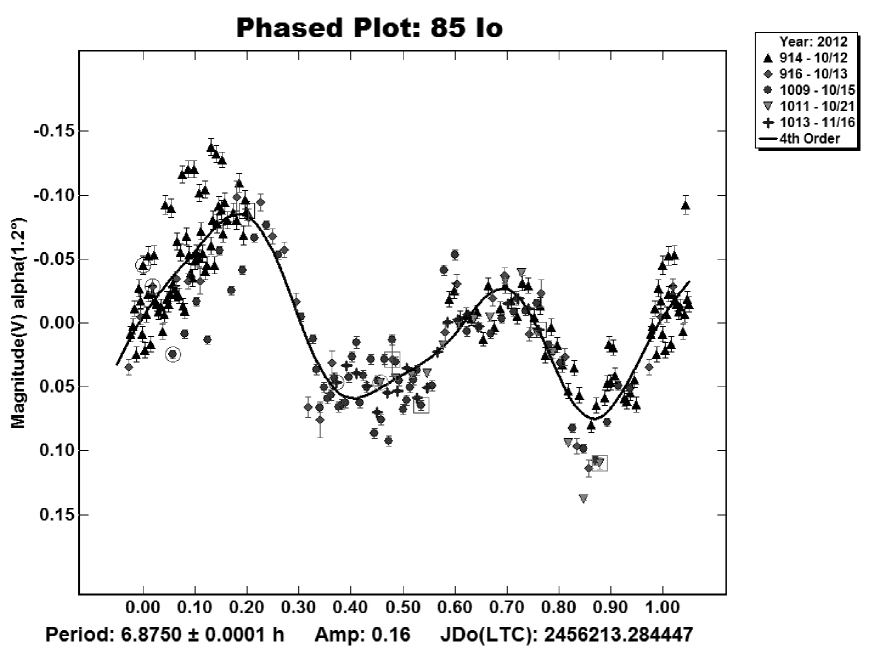
Figure 1: First reference lightcurve for asteroid (85) Io ($JD_{0}$ = 2456214.50).

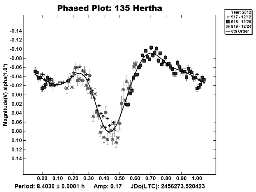
Figure 2: Reference lightcurve for asteroid (135) Hertha ($JD_{0}$ = 2456280.50)).

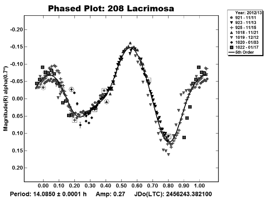
Figure 3: Reference lightcurve for asteroid (208) Lacrimosa ($JD_{0}$ = 2456264.50).

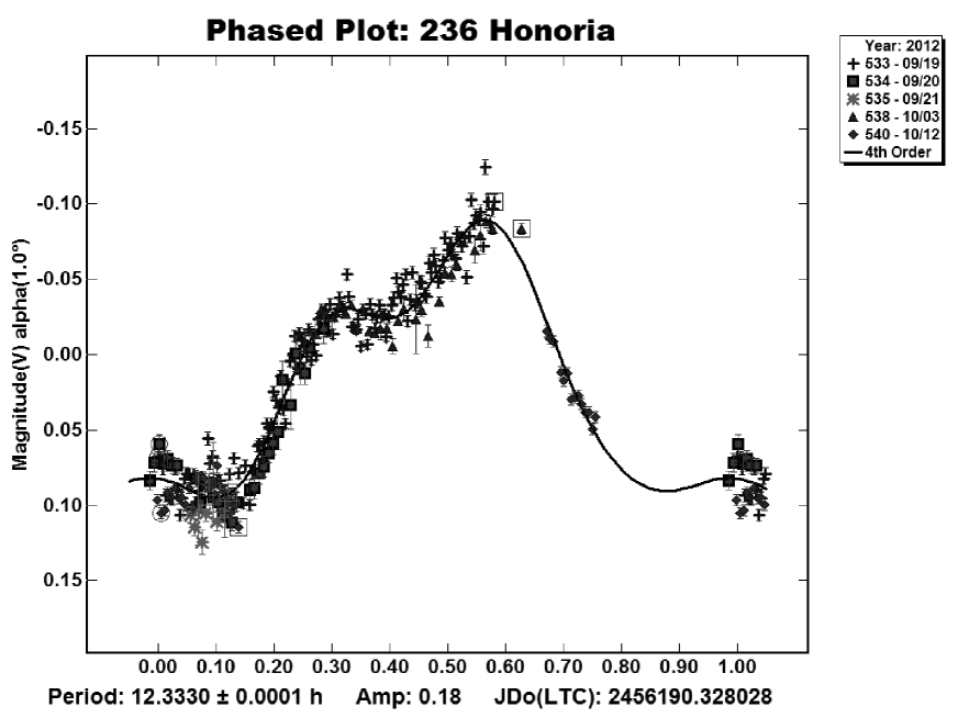
Figure 4: First reference lightcurve for asteroid (236) Honoria ($JD_{0}$ = 2456197.50).

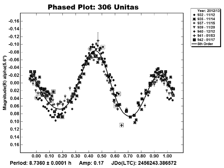
Figure 5: Reference lightcurve for asteroid (306) Unitas ($JD_{0}$ = 2456255.50).

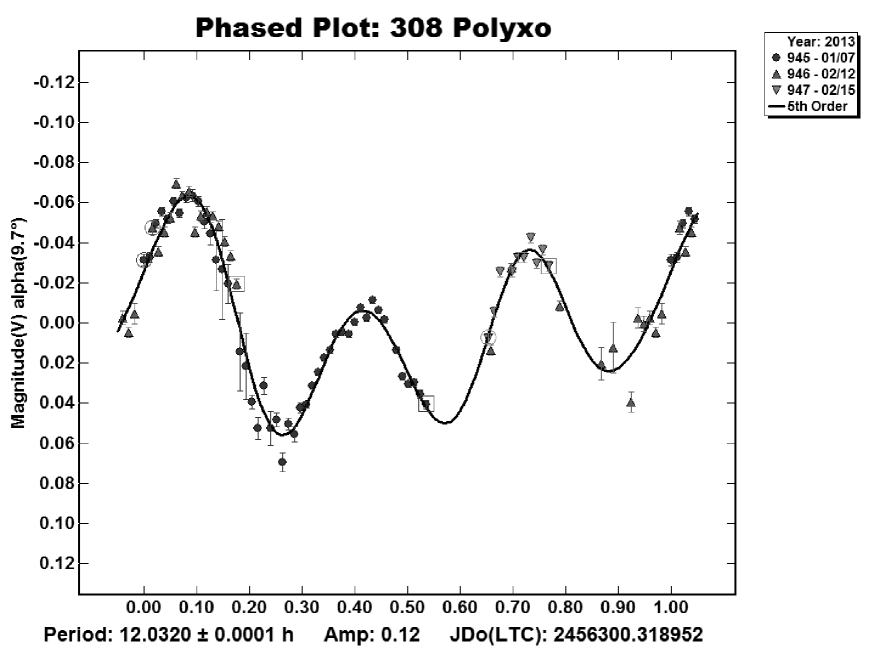
Figure 6: Reference lightcurve for asteroid (308) Polyxo ($JD_{0}$ = 2456306.50).

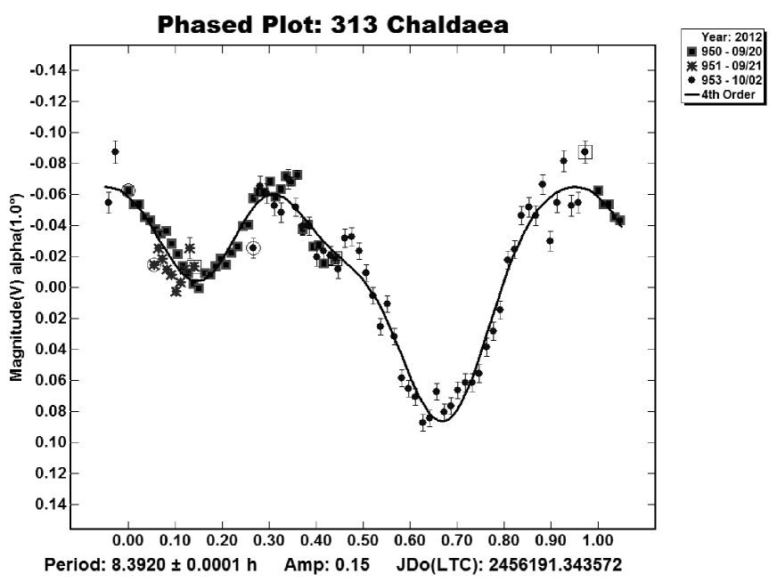
Figure 7: First reference lightcurve for asteroid (313) Chaldaea ($JD_{0}$ = 2456197.50).

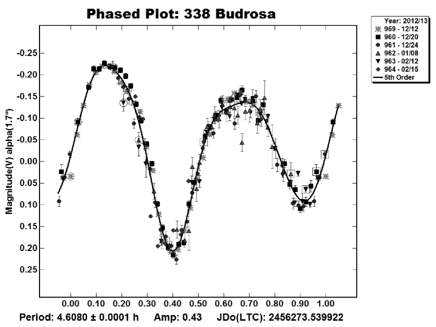
Figure 8: Reference lightcurve for asteroid (338) Budrosa ($JD_{0}$ = 2456295.50).

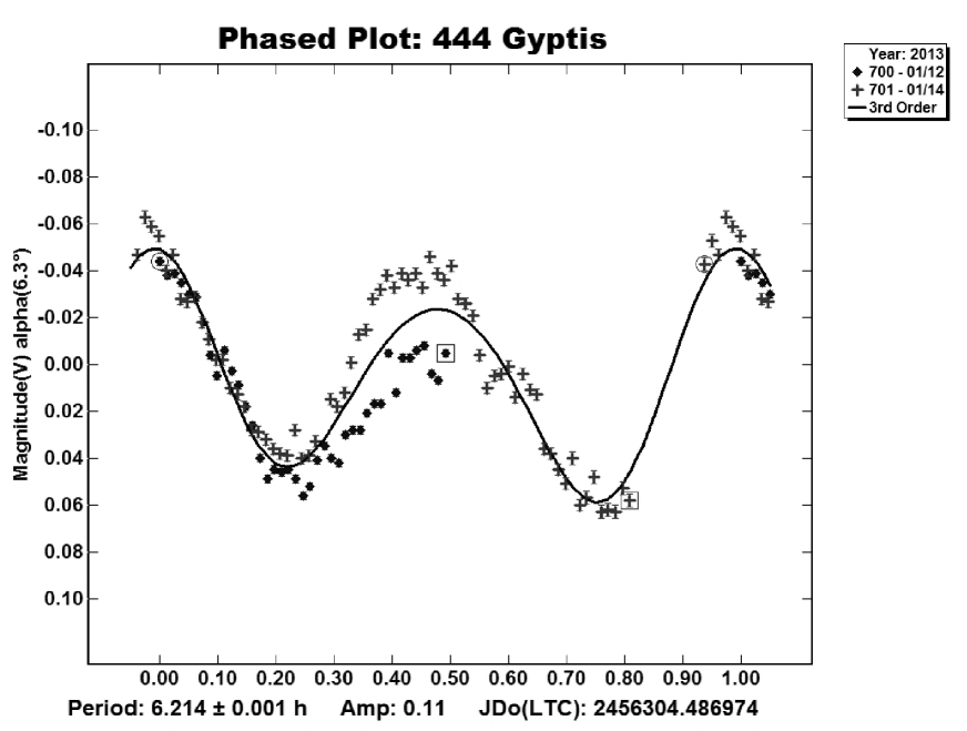
Figure 9: The suspect binary event in lightcurve of (444) Gyptis.

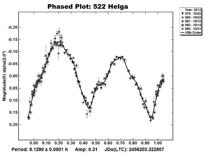
Figure 10: First reference lightcurve for asteroid (522) Helga ($JD_{0}$ = 2456209.50).

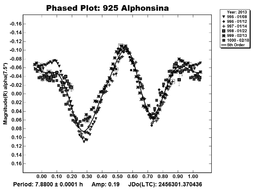
Figure 11: Reference lightcurve for asteroid (925) Alphonsina ($JD_{0}$ = 2456318.50).

For each asteroid in our observing program, we obtained a maximum possible number of lightcurves taken at different phase angles, as allowed by weather conditions and available telescope time. All data were obtained, for each object, at the same apparition, so they all correspond to a unique value of the aspect angle (the angle between the line of sight and the direction of the rotation pole of the object).

Observations were performed between September 2012 and February 2013. We used an 810mm f/7.9 modified Ritchey-Chrétien reflector on a fork equatorial mount combined with a back illuminated CCD camera, 2048 $\times$ 2048 square pixel with size of 15 micron. The CCD was used in binning mode 2 $\times$ 2 with a FOV (Field Of View) of 16.5 $\times$ 16.5 arcmin. The telescope was equipped with a filter wheel with standard $B$, $V$, $R$, $I$ and $C$ (clear) filters. The work at the telescope was divided in two steps:

• Asteroid photometric observations in $V$ and $R$ band.

• Calibration of FOVs Landolt standard fields in $V$ and $R$ (all–sky photometry).

Reduction of the data and lightcurve analysis were done using MPO Canopus v10.7 , a software package which carries out differential aperture photometry and Fourier period analysis using an algorithm developed by Harris et al. (1989). In all cases, the computed rotation period of the targets was found to be in good agreement with the known value available in the literature. Calibrated $V$ and $R$ magnitudes of the target asteroids were obtained from calibrated photometry of the adopted comparison stars, based on measurements of Landolt calibration fields (see below). Note that we used $R$ measurements for the purposes of the determination of atmospheric extinction (which depends upon the $V-R$ colour index), only, and we did not use them for the purposes of building phase - mag curves. The resulting, calibrated $V$ magnitudes of the asteroids were converted to unit distance from both the Sun and the observer.

As all asteroids rotate, typically with periods from a few hours to a few days, they should all show some rotational modulation superposed on top of the phase curve. Without correction, these rotational modulations will cause deviations from a smooth phase curve.

For each object, a full lightcurve was obtained by merging together, whenever possible, phase-calibrated magnitudes taken in consecutive nights at approximately the same phase angle. A Fourier best-fit was computed to derive the lightcurve morphology, in particular the magnitude values at the lightcurve maximum and minimum $m_{V}(max)$ and $m_{V}(min)$. These reference lightcurves, shown in Figs. 1 - 11, were then used to compute the rotational phases and phase-dependent magnitude shifts of a number of partial lightcurves of the same object taken at different phase angles, whenever a full lightcurve could not be obtained in the same night due to time or wheather constraints. In so doing, each night of observation could be eventually used to derive values for $m_{V}(max)$ and $m_{V}(min)$, and use them to build the phase - mag curves.

In this work we were mainly interested in comparing different photometric systems between them. To do this we used in our analysis the magnitudes corresponding to lightcurve maxima, although we are aware that we could have used instead the magnitudes at lightcurve minima or, as done in papers of other authors, the mean magnitudes, that can be in principle the best option. On the other hand, taking into account that we did not obtain at each epoch and for each object complete lightcurves, as explained above, something that certainly introduces some uncertainty, we do not think that the main results of this analysis are strongly dependent upon our choice of working in terms of lightcurve maxima. When looking at our results, however, one should take into account that we use the symbol $H$ to refer to maximum brightness, and not to lightcurve-averaged values.

The implicit requirement of this approach is that the morphology of the lightcurve does not change substantially at different phase angles. For sake of safety, in most cases two (or three, as in the case of (313) Budrosa) distinct Fourier reference lightcurves were obtained, one at low and another at high phase angle. For more details see A. We note that not all our reference lightcurves are of the same quality. In some cases, the data obtained in consecutive nights do not fit perfectly with each other, and this effects seems to be larger than one would expect by considering the pure effect of little differences in phase angle. These effects, quite usual in asteroid phtometry, may be due to different reasons, mostly related to changes in atmospheric conditions. As a general rule, however, the reference lightcurves are reasonably stable and well defined.

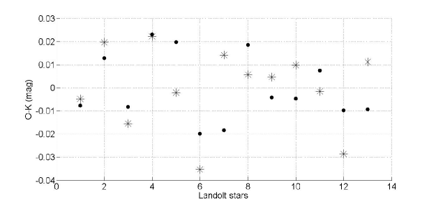
Figure 12: Comparison between the observed (O) and known (K) magnitudes of the Landolt stars used on 2012, Oct 22 to compute the atmospheric model used to reduce the observations of the asteroid 236 Honoria (asterisk = $R$ filter, dots = $V$ filter).

4.1 The Landolt field calibration

Every time the night was photometric, we carried out photometric measurements of Landolt field stars in $V$ and $R$ to derive a correct calibration of the instrumental magnitudes. This was done to derive reliably calibrated magnitudes of the comparison stars used to derive the correspondingly calibrated magnitudes of the asteroids for each night of observation. Of course, the comparison stars are in the same FOV as the asteroid. Images of various Landolt fields were taken at various air masses in order to calibrate the atmospheric extinction (Harris et al., 1981).
We then measured the $V$ and $R$ instrumental magnitude for each Landolt star by computing the average of $5$ images per filter. From the instrumental magnitude, a four parameters atmospheric model was fit using the following linear equations:

$$V-v=-[k_{1v}+k_{2v}(V-R)]X+c_{v}(V-R)+V_{0}$$ (2)

$$R-r=-[k_{1r}+k_{2r}(V-R)]X+c_{r}(V-R)+R_{0}$$ (3)

where: $k_{1}$ is the first-order atmospheric extinction for the V or R filter; $k_{2}$ is the second-order atmospheric extinction for the given filter; $c$ is the instrumental color correction coefficient for the given colour index; $R_{0}$ and $V_{0}$ are the unknown zero point magnitudes; $V$, $R$ and $V-R$ are the known, tabulated magnitudes and color index from Landolt fields; $v$ and $r$ are the measured instrumental magnitudes; $X$ is the air-mass, i.e. the optical path length through the Earth’s atmosphere, expressed as a ratio relative to the path length at the zenith.

To get the four unknown coefficients it is sufficient to have at least four different Landolt stars, so that we can write Eqn. (2) and Eqn. (3) for each star and get a system of linear equations to be solved. In general, to increase the accuracy, we processed about ten stars in such a way to have an overdetermined linear system. The method of ordinary least squares was then used to find an approximate solution.

After finding the various constant parameters of the atmospheric model, we derived the calibrated $V$ and $R$ magnitudes of the comparison stars used to compute asteroids’ magnitudes. We show in Fig.  12 a comparison between the observed and known magnitude of stars located within some of the considered Landolt fields analyzed to process the observations of asteroid (236) Honoria. The resulting $O-C$ differences are at most few hundredths of a magnitude both in $V$ and in $R$ filter.

In applying this data reduction procedure we assumed that the $V-R$ of the comparison stars are about equal (within few hundredths of mag) to the $V-R$ of the asteroid. For this reason, we used as comparison star only solar-type stars. Under this assumption, from Eqn. (2) and Eqn. (3)) we obtain ($a$=asteroid, $c$=comparison star):

$$V_{c}-V_{a}=v_{c}-v_{a}$$ (4)

$$R_{c}-R_{a}=r_{c}-r_{a}$$ (5)

Table 2: Summary of the lightcurve analysis for our sample of asteroids. $V_{max}$ is the reduced magnitude of the lightcurve maximum, $V_{min}$ is the reduced magnitude of the lightcurve minimum, $V_{mean}$ is the mean magnitude of the lightcurve while $\sigma_{m}$ is the standard deviation of the mean between the Fourier fit and the observed magnitudes.

Phase angle (∘)	$V_{max}$ (mag)	$V_{min}$ (mag)	$V_{mean}$ (mag)	$\sigma_{m}$ (mag)
236 Honoria
1.27	8.17	8.35	8.27	0.06
1.95	8.22	8.40	8.32	0.06
0.86	8.10	8.28	8.20	0.09
6.39	8.63	8.82	8.74	0.05
9.77	8.73	8.91	8.83	0.06
10.69	8.78	8.97	8.89	0.07
22.14	9.12	9.30	9.22	0.04
24.72	9.16	9.34	9.27	0.05
313 Chaldea
0.99	9.06	9.21	9.11	0.02
0.57	8.94	9.09	8.99	0.01
4.74	9.21	9.36	9.26	0.05
8.37	9.41	9.53	9.46	0.04
10.50	9.54	9.66	9.60	0.05
20.33	9.86	9.99	9.94	0.06
522 Helga
2.00	9.23	9.54	9.37	0.08
2.19	9.28	9.59	9.42	0.09
4.07	9.36	9.67	9.50	0.11
4.99	9.41	9.72	9.55	0.08
7.40	9.55	9.86	9.69	0.09
13.67	9.85	10.14	9.99	0.12
16.24	9.88	10.17	10.11	0.13
85 Io
0.89	7.62	7.80	7.73	0.06
1.18	7.67	7.85	7.77	0.07
2.07	7.82	8.00	7.92	0.04
5.11	8.01	8.19	8.11	0.05
16.24	8.48	8.66	8.58	0.04
17.49	8.53	8.76	8.65	0.08
21.24	8.66	8.89	8.78	0.08

Table 2: (continued). Summary of the lightcurve analysis for our sample of asteroids.

Phase angle (∘)	$V_{max}$ (mag)	$V_{min}$ (mag)	$V_{mean}$ (mag)	$\sigma_{m}$ (mag)
208 Lacrimosa
0.64	9.20	9.48	9.33	0.04
1.01	9.24	9.52	9.37	0.07
1.74	9.39	9.66	9.52	0.08
3.75	9.69	9.96	9.82	0.09
11.85	9.73	10.01	9.87	0.08
17.28	9.97	10.25	10.10	0.08
19.18	9.99	10.27	10.12	0.08
306 Unitas
5.45	9.18	9.37	9.28	0.07
5.83	9.17	9.36	9.27	0.05
6.34	9.21	9.39	9.31	0.05
8.00	9.28	9.46	9.38	0.02
16.03	9.61	9.79	9.71	0.06
21.23	9.60	9.78	9.70	0.10
22.85	9.69	9.87	9.79	0.05
338 Budrosa
1.54	8.74	9.16	8.93	0.16
3.86	8.93	9.36	9.12	0.14
10.89	9.49	9.91	9.68	0.11
18.93	9.85	10.28	10.04	0.11
19.25	9.77	10.20	9.97	0.16
925 Alphonsina
7.16	8.84	9.01	8.92	0.07
8.15	8.79	8.97	8.87	0.05
9.22	8.87	9.05	8.96	0.06
12.16	9.03	9.21	9.11	0.03
18.93	9.17	9.35	9.25	0.05
20.04	9.11	9.29	9.19	0.05

5 Asteroid photometric systems

Here we briefly summarize some of the most commonly adopted photometric systems to describe the observed phase - mag curves of asteroids. By knowing the orbit, and hence the distance of an asteroid observed at a given epoch, if we call $\alpha$ the phase angle and $m_{V}$ the measured apparent magnitude, we can immediately compute $V(\alpha,1)$, namely the conversion of $m_{V}$ into the magnitude corresponding to unit distance from both the Sun and the observer:

$$V(\alpha,1)=m_{V}-5\,log_{10}\left(r\Delta\right)$$ (6)

where $r$ is the asteroid heliocentric distance, and $\Delta$ is the distance from the observer, both distances being expressed in AU. Since in this paper we always use magnitudes reduced to unit distance, let us simplify the notation by writing henceforth $V(\alpha)$ instead of $V(\alpha,1)$.

In analyzing our data, we have considered three main photometric systems that are or have been used in asteroid science to describe the variation of $V(\alpha)$ as a function of $\alpha$. The first one is the so-called $(H,G)$ system, that was officially adopted by the International Astronomical Union between 1985 and 2012 (Bowell et al., 1989). By indicating as $H$ the value of $V(0^{\circ})$, namely, by definition, the absolute magnitude of the asteroid, the $(H,G)$ system is defined by the following Equation:

$$V(\alpha)=H+2.5\,log_{10}\left[\left(1-G\right)\Phi_{1}(\alpha)+G\Phi_{2}(\alpha)\right]$$ (7)

where the so-called slope parameter $G$ is a function describing the variation of $V(\alpha)$ measured at different phase angles. $\Phi_{1}(\alpha)$ and $\Phi_{2}(\alpha)$ are two ancillary functions of the phase angle $\alpha$, with $\Phi_{1}(0^{\circ})=\Phi_{2}(0^{\circ})\equiv 1$. A comprehensive description of the $(H,G)$ system, including an explicit mathematical formulation of the $\Phi_{1}$ and $\Phi_{2}$ functions of $\alpha$, can be found in Muinonen et al. (2010).

The second photometric system that we consider in this paper is the $(H,G_{1},G_{2})$ system, that has been more recently proposed by Muinonen et al. (2010) as an improvement of the older $(H,G)$ system, and has been later officially adopted by the IAU during the General Assembly in 2012. It is defined as:

$$V(\alpha)=H+2.5\,log_{10}\left[G_{1}\overline{\Phi}_{1}(\alpha)+G_{2}\overline{\Phi}_{2}(\alpha)+\left(1-G_{1}-G_{2}\right)\overline{\Phi}_{3}(\alpha)\right]$$ (8)

where $\overline{\Phi}_{1}(\alpha)$, $\overline{\Phi}_{2}(\alpha)$ and $\overline{\Phi}_{3}(\alpha)$ are three base functions of the phase angle $\alpha$, with $\overline{\Phi}_{1}(0^{\circ})=\overline{\Phi}_{2}(0^{\circ})=\overline{\Phi}_{3}(0^{\circ})\equiv 1$ A comprehensive description of this photometric system, that has been proposed to improve the accuracy of the derived values of H, is given by Muinonen et al. (2010). A constrained non linear least-squares algorithm to be used in estimating the parameters in the ($H$, $G_{1}$, $G_{2}$) phase function has been published more recently by Penttilä et al. (2016). Note that we decided to consider only the full ($H$, $G_{1}$, $G_{2}$) phase function in this paper, and we did not use the simplified ($H$, $G_{12}$) phase function that can replace ($H$, $G_{1}$, $G_{2}$) when the coverage of the phase - mag is not optimal. We took this decision because since the beginning our goal was to obtain reasonably well-sampled phase - mag curves, suitable to derive the full set of $H$, $G_{1}$ and $G_{2}$ parameters. Although in few cases this was not really possible, we decided that adding the simplified system would not have been so advantageous.

Moreover, we also consider the empirical photometric system proposed by Shevchenko (1997), expressed through the following Equation:

$$V(\alpha)=V_{lin}(0)-\frac{a}{1+\alpha}+b\alpha$$ (9)

In this formulation, the opposition effect corresponds to the difference between a simple extrapolation to zero phase of the linear part of the mag - phase curve, described by the $b$ parameter, and the value that is actually observed and is determined by the presence of a brightness surge described by the term including the parameter $a$. $V_{lin}(0)$ represents therefore the extrapolation to zero phase angle of a purely linear mag - phase relation having angular coefficient $b$. The absolute magnitude, taking into account the presence of an opposition effect, is then given by $H=V_{lin}(0)-a$, $a$ and $b$ being parameters to be determined for each object. Note also that the form of the term with $a$ in Eqn. 9 is such that the profile of the opposition effect has a fixed shape, determined by the adopted form for the denominator: for instance, at the phase of $1^{\circ}$ the magnitude opposition effect becomes about one half the value assumed at zero phase angle. In principle, this might be changed, although we do not make any attempt to explore alternative formulations.

Finally, we note that we also computed simple linear least-squares fits for the objects of our sample, but using only observations obtained at phase angle $\alpha\geq 10^{\circ}$. The reason was to explore the relation between such kind of slope, that will be routinely determined by Gaia observations, and the albedo, to improve the calibration of the proposed Belskaya & Shevchenko (2000) relation.

6 The results

We built our Phase - mag curves by using as magnitude values those corresponding to the maxima of the obtained lightcurves. In particular, we estimated that in all the different cases the uncertainty in the determination of this parameter was not exceeding $\pm 0.015$ mags. Therefore, we adopted this value in the computations of the best-fit representations of our phase - mag curves using the different photometric systems described above.

Apart from an easy computation to determine the slope $\beta$ of a linear relation between magnitude and phase for phase angles $>10^{\circ}$, in the most difficult case of the three main photometric systems described in the previous Section, nonlinear regression methods were needed. In our case, we used different independent approaches, and we checked that the results were coincident within the nominal error bars.

A first approach was the use of a genetic algorithm developed in the past by some of us for other purposes, and optimized for the present problem. Genetic algorithms are relatively simple and are well suited to determine sets of best-fit parameters using even more complicated relations than those considered in this application. These algorithms have the advantage of making an extensive exploration of the parameters’ space, and to be scarcely prone to fall into local best-fit minima. The draw-back is some difficulty in estimating the resulting uncertainties of the solution parameters. Essentially the same approach, originally developed for the purpose of inversion of sparse asteroid photometric data (Cellino et al., 2009) has also been more recently used in the computation of best-fit approximation of asteroid phase - linear polarization data (Cellino et al., 2015, 2016).

In order to obtain independent results and to obtain a better estimate of the uncertainties on the derived parameters of the different photometric systems, we adopted also more classical least-squares approaches by using standard numerical routines available in the literature and implementing them in algorithms either written by ourselves, or using, as a check, routines included in the MATLAB^® package by MathWorks. In particular, we used the MATLAB statistical toolbox “nlinfit”, that uses a minimisation tool based on the Levenberg-Marquardt algorithm. We also note that, in fitting our data using the ($H$, $G_{1}$, $G_{2}$) system, we followed the procedures recommended by Penttilä et al. (2016), apart from the fact that in a few cases we allowed the value of either $G_{1}$ or $G_{2}$ to reach negative values, provided that, in any case, $1-G_{1}-G_{2}\leq 1$

The results obtained with the different approaches were found to be in good agreement, giving coincident results within the derived error bars. We also note that for some objects no solution could be found using one or more of the adopted photometric systems. This happened in the cases of asteroids (306) Unitas and (925) Alphonsina, for which the low-phase angle region was not adequately covered by our observations making it impossible to obtain a best-fit solution using the ($H$, $G_{1}$, $G_{2}$) photometric system. In this respect, we remind that the ($H$, $G_{1}$, $G_{2}$) system has been developed precisely to improve the accuracy in the determination of the absolute magnitude $H$, taking into account the behaviour exhibited by the objects at small phase angles.

Conversely, in the case of (338) Budrosa, we could not compute a simple linear fit, due to a lack of data at large phase angles. Among the other asteroids of our original target list shown in Table 1, we were forced to exclude a priori from our analysis (135) Hertha, due to an insufficient number of data points. We also discarded (308) Polyxo and (444) Gyptis due to problems of data quality. In particular, in the case of Gyptis we obtained some anomalous lightcurve morphology on January 13-14, 2013, when we observed a magnitude variation looking like a mutual event in a binary system (Fig. 9). This is certainly to be confirmed by future observations, but it is clear that in any case the possible presence of mutual events would alter the lightcurve morphology, therefore we did not take into account this asteroid for any further analysis in this paper.

The results of our best-fit computations using the ($H,G$), ($H,G_{1},G_{2}$) and the Shevchenko systems are shown in Figs. 13–19. In all the figures, the best-fit obtained using the ($H,G$), ($H$, $G_{1}$, $G_{2}$), and Shevchenko photometric systems are shown using different colours. We show also the linear best-fits of the measurements obtained at phase angles larger than $10^{\circ}$, for the objects having at least three measurements in this interval. We remind that $10^{\circ}$ is approximately the lower limit in phase angle attainable by Gaia observations of main belt asteroids. We are therefore interested in studying how a simple linear fit of data obtained at phase angles $>10^{\circ}$ can be used to derive some information about the main properties of the phase - mag curves, and in particular how the slopes of these linear fits can be used to derive reasonable values for the geometric albedo.

The obtained best-fit parameters corresponding to the different photometric systems considered in this paper are also listed in Tables 3 - 6. Note that asteroid (925) Alphonsina is not included in Table 4, because no ($H$, $G_{1}$, $G_{2}$) fit could be found for this object. The average rms residuals of the phase - mag data of each object in our sample, obtained using the three different photometric systems, are listed in Table 6.

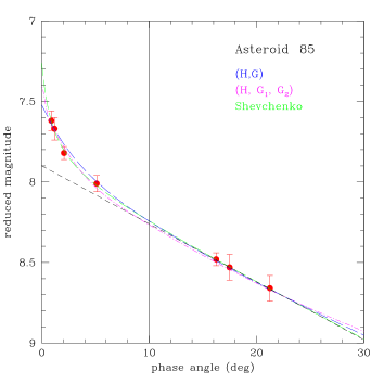
Figure 13: Magnitude maximum brightness - phase curve in $V$ band for (85) Io, and resulting best-fit curves corresponding to the three photometric systems considered in this paper. Left Panel: whole curve. The vertical line separates the range of phase angles smaller than $10^{\circ}$, the lower limit in phase angle attainable by Gaia. The linear fit of the measurements obtained above $10^{\circ}$ are also shown. Right Panel: zooming on the solar opposition region, at phase angle $\leq$ 10 degrees

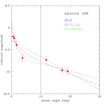
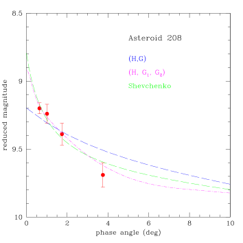
Figure 14: The same as Fig. 13, but for asteroid (208) Lacrimosa. Note that the point at phase angle of 3.75 degrees is responsible of the negative value of the $G_{1}$ parameter found in the best-fit solution.

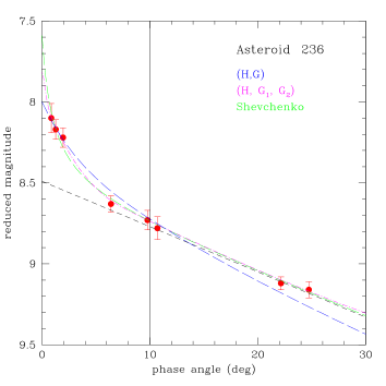
Figure 15: The same as Fig. 13, but for asteroid (236) Honoria.

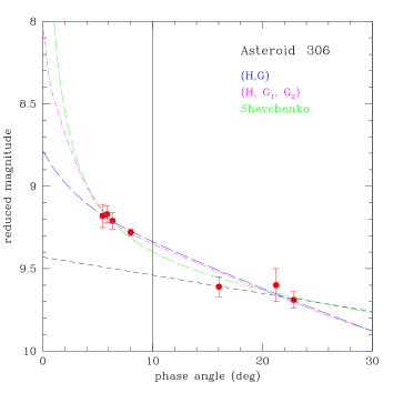
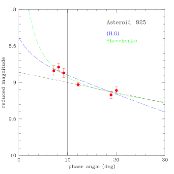
Figure 16: Left Panel: Magnitude maximum brightness - phase curve in $V$ band for (306) Unitas, and resulting best-fit curves corresponding to the three photometric systems considered in this paper. The region at small phase angles is poorly sampled, leading to big differences in the derived values of $H$, and is shown separately. Right Panel: the same, but for asteroid (925) Alphonsina. For this object, no solution using the ($H$, $G_{1}$, $G_{2}$) photometric system could be found. Not that for both objects, the linear fit of data at phase angles $>10^{\circ}$ are also shown.

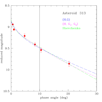
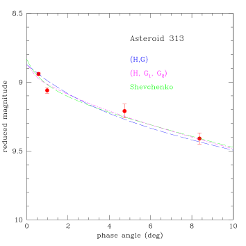
Figure 17: The same as Fig. 13, but for asteroid (313) Chaldaea. Note that for this asteroid, only two measurements have been obtained at phase angles $>10^{\circ}$, therefore no linear-fit of these measurements has been computed.

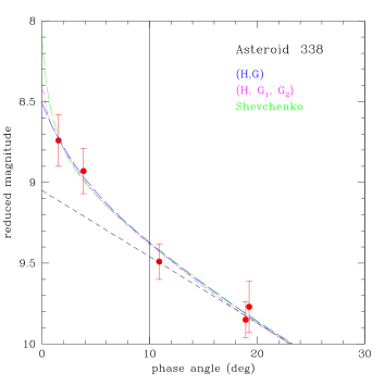
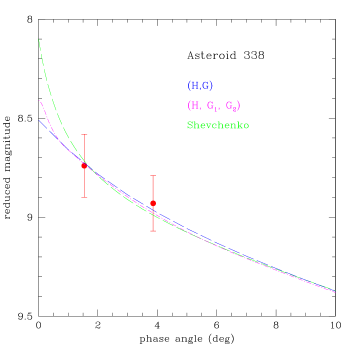
Figure 18: The same as Fig. 13, but for asteroid (338) Budrosa. Only two observations cover the phase angle interval between $0^{\circ}$ and $10^{\circ}$.

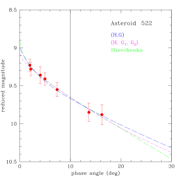
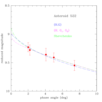
Figure 19: The same as Fig. 13, but for asteroid (522) Helga. As in the case of (313) Chaldaea, only two measurements have been obtained at phase angles $>10^{\circ}$, and no linear-fit of these measurements has been computed.

Table 3: Results of the best-fit solutions of the phase-mag maximum brightness curves using the $(H,G)$ photometric system.

object	N(obs)	$H$	$G$	rms (mag)
85	7	$7.52\pm 0.10$	$0.0753\pm 0.0210$	0.022
208	7	$9.20\pm 0.45$	$0.2761\pm 0.0853$	0.085
236	8	$8.00\pm 0.14$	$0.0715\pm 0.0311$	0.053
306	7	$8.79\pm 0.27$	$0.2891\pm 0.0452$	0.043
313	6	$8.87\pm 0.28$	$0.1954\pm 0.0512$	0.043
338	5	$8.51\pm 0.18$	$-0.0812\pm 0.0437$	0.046
522	7	$9.00\pm 0.16$	$0.1411\pm 8.0317$	0.027
925	6	$8.39\pm 0.48$	$0.3498\pm 0.0830$	0.047
average				0.046

Table 4: Results of the best-fit solutions of the phase-mag maximum brightness curves using the $(H,G_{1},G_{2})$ photometric system.

object	N(obs)	$H$	$G_{1}$	$G_{2}$	rms (mag)
85	7	$7.41\pm 0.08$	$0.3358\pm 0.0401$	$0.2147\pm 0.0298$	0.022
208	7	$8.92\pm 0.07$	$-0.3116\pm 0.0675$	$0.6598\pm 0.0418$	0.053
236	8	$7.82\pm 0.06$	$0.1155\pm 0.0331$	$0.3436\pm 0.0223$	0.019
306	7	$8.04\pm 0.43$	$-0.1309\pm 0.4369$	$0.3624\pm 0.6269$	0.043
313	6	$8.88\pm 0.08$	$0.6240\pm 0.0386$	$0.1510\pm 0.0336$	0.026
338	5	$8.41\pm 0.10$	$0.5607\pm 0.0457$	$-0.0037\pm 0.0365$	0.047
522	7	$9.07\pm 0.12$	$0.7302\pm 0.0623$	$0.0879\pm 0.0450$	0.020
average					0.033

Table 5: Results of the best-fit solutions of the phase-mag maximum brightness curves using the Shevchenko photometric system.

object	N(obs)	$V(1,0)$	$a$	$b$	$H=V(1,0)-a$	rms (mag)
85	7	$7.96\pm 0.03$	$0.70\pm 0.07$	$0.035\pm 0.002$	$7.26\pm 0.07$	0.009
208	7	$9.74\pm 0.03$	$0.95\pm 0.06$	$0.014\pm 0.002$	$8.79\pm 0.07$	0.060
236	8	$8.56\pm 0.02$	$0.97\pm 0.05$	$0.026\pm 0.001$	$7.59\pm 0.05$	0.030
306	7	$9.60\pm 0.09$	$3.23\pm 0.53$	$0.009\pm 0.003$	$6.37\pm 0.54$	0.033
313	6	$9.13\pm 0.02$	$0.30\pm 0.05$	$0.037\pm 0.002$	$8.83\pm 0.05$	0.033
338	5	$9.00\pm 0.04$	$0.90\pm 0.11$	$0.045\pm 0.002$	$8.10\pm 0.12$	0.053
522	7	$9.29\pm 0.04$	$0.39\pm 0.12$	$0.040\pm 0.002$	$8.90\pm 0.13$	0.025
925	6	$9.21\pm 0.15$	$3.74\pm 1.00$	$0.006\pm 0.006$	$5.47\pm 1.01$	0.042
average						0.036

Table 6: Results of the best-fit solutions of the phase-mag maximum brightness curves using a simple linear relation for observations at phase angle $>10^{\circ}$. Objects having a number N(obs) $<3$ of measurements at phase angle $>10^{\circ}$ were not included in the analysis.

object	N(obs)	$\beta$	rms (mag)
85	3	$0.036\pm 0.001$	0.003
208	3	$0.037\pm 0.007$	0.022
236	3	$0.028\pm 0.002$	0.014
306	3	$0.011\pm 0.012$	0.036
338	3	$0.041\pm 0.010$	0.040
925	3	$0.014\pm 0.008$	0.031
average			0.024

7 Discussion

The results shown in the previous Section indicate that the old (H, G) system gives the worst residuals when it is adopted to fit our limited sample of phase - mag data. This is not unexpected, because both the ($H$, $G_{1}$, $G_{2}$) and the Shevchenko photometric systems have been developed to replace (H, G), and provide better fits of existing data, and in particular more accurate estimates of the absolute magnitudes.

In terms of average residuals, listed in Table 6, at face values the best-fits obtained using ($H$, $G_{1}$, $G_{2}$) are slightly better than in the case of using the Shevchenko photometric system, but the differences are really small. By looking at Figs. 13–19, however, one can see that in terms of the resulting value of the absolute magnitude $H$, the differences can be non-negligible, attaining typical values of 0.2 mag in most cases. In a couple of cases, however, we obtained an ($H$, $G_{1}$, $G_{2}$) best-fit solution with a negative value for either $G_{1}$ or $G_{2}$. We cannot rule out the possibility that in these cases the obtained phase - mag curves could include some abnormal magnitude value, obliging the flexible ($H$, $G_{1}$, $G_{2}$) system to obtain a best-fit representation including anomalous values for some of its parameters. Even in the other cases, however, the resulting differences in $H$ are not negligible. By looking at the plots shown in Figs. 13–19 it turns out that the $H$ value found by using the Shevchenko photometric system is systematically brighter than the value corresponding to an ($H$, $G_{1}$, $G_{2}$) (and, even more, the (H, G)) solution. At least in some cases, a purely visual inspection of the data would suggest that the ($H$, $G_{1}$, $G_{2}$) best-fit solution looks slightly more credible, but this is not, of course, an acceptable criterion. At face value, the average rms values indicate that the Shevchenko-based fits are sligthly worse, but the differences do not appear to be sufficient to conclude that the $H$ values given by the ($H$, $G_{1}$, $G_{2}$) system are more realistic.

We also note that, if we make a comparison between the values of the linear coefficient $\beta$ of a purely linear best-fit of data, taking into account only lightcurves obtained at phase angles $>10^{\circ}$ (shown in Table 6) and the corresponding value of the $b$ parameter in the Shevchenko system (listed in Table 5), we can see that in most cases, including asteroids (85), (236), (338), and (925), there is a good agreement. In only one case, that of (208), the differences are significant. In this case, however, it seems that the difference between $b$ and $\beta$ would tend to disappear if the point of the phase - mag curve at $3.75^{\circ}$, which is also responsible of the negative value derived for the $G_{1}$ parameter, would be removed.

These results, though very preliminary, tend to suggest that using a simple linear fit of data obtained at large phase angles, as in the case of Gaia asteroid data, could lead in many cases to linear coefficient values that would be in reasonable agreement with the linear part of the phase - mag curve derived by the more refined Shevchenko photometric system. The latter takes into account the existence of a non-linear brightness surge at small phase angles, and it would not be obvious a priori that the corresponding values of the linear part of the Shevchenko system must be necessarily found to be in good agreement with a simple linear fit of data not including magnitude values affected by the opposition effect. This can be an important result from the point of view of the future treatment of Gaia data, in the case a relation between geometric albedo and the slope of a linear variation of the phase - mag curves will be used to determine estimates of the albedo from Gaia data. The point is that the relation suggested by Belskaya & Shevchenko (2000) was based on the use of the $b$ parameter of the Shevchenko photometric system, and not on a simple $\beta$ slope obtained from an analysis based on large-phase data, only.

Table 7: Results of the linear best-fit solutions for the relations $y=m\,\log_{10}(p_{V})+q$ where $p_{V}$ is the geometric albedo and $y$ represents the photometric parameters indicated in column 1. $N_{curves}$ is the number of phase - mag curves used in computing the linear best-fit.

y	$N_{curves}$	$m$	$q$	Correlation
$G_{1}$	36	$-0.6855\pm 0.1019$	$-0.1383\pm 0.0907$	0.756
$G_{2}$	36	$0.5445\pm 0.0571$	$0.7299\pm 0.0508$	0.853
$b$	23	$-0.0241\pm 0.0041$	$0.0135\pm 0.0035$	0.790
$\beta$	7	$-0.0152\pm 0.0060$	$0.0196\pm 0.0057$	0.748

Figure 20: results of the best-fit computations for the relations of the kind $y=m\,\log_{10}(p_{V})+q$ where $p_{V}$ is the geometric albedo and $y$ represents the photometric parameters $G_{1}$ (top.left), $G_{2}$ (top-right), $b$ (bottom-left) and $\beta$ (bottom-right), respectively. See the text for the meaning of the above parameters.

In this respect, following Shevchenko et al. (2016), we explored some possible relations between photometric parameters and geometric albedo, taking profit of the data published by the above authors. In particular, we considered relation of the type:

$$y=m\,\log_{10}(p_{V})+q$$ (10)

where $p_{V}$ is the geometric albedo, and $y$ is one among $G_{1}$, $G_{2}$, $b$, and $\beta$. With respect to the analysis performed by Shevchenko et al. (2016), a difference is that, in our analysis we do not use albedo values coming from WISE thermal radiometry data, because we think that these data can be affected by too big uncertainties to be used for calibration purposes, for the reasons explained by Cellino et al. (2015). Instead, in the present analysis we use albedo values computed either by exploiting the proposed $\Psi$ - albedo relation, where $\Psi$ is the polarimetric parameter proposed by Cellino et al. (2015), and computed for a sample of asteroids for which we have estimates of the $G_{1}$, $G_{2}$ and $b$ photometric parameters, either given by Shevchenko et al. (2016), or found in the present paper. We adopt values of $\Psi$ based on the results of Cellino et al. (2016), whenever possible updated using still unpublished polarimetric values obtained by the Calern Asteroid Polarimetric Survey (CAPS) (Devogèle et al., 2017). In some cases in which the polarimetric $\Psi$ parameter is not known, we use the albedo values published by Shevchenko & Tedesco (2006).

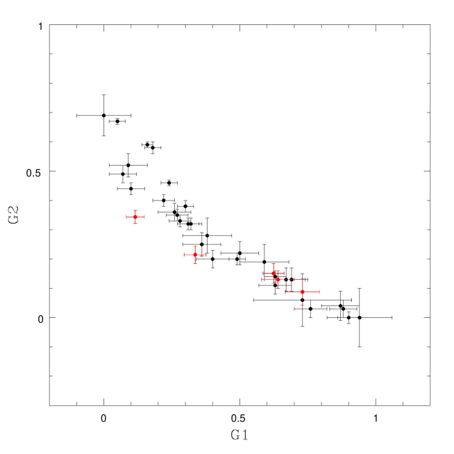
Figure 21: Plot of the relation between the $G_{1}$ and $G_{2}$ best-fit parameters. The points in red indicate four objects for which the values of the parameters could be derived from the observations presented in this paper (asteroids (85), (236),(313) and (522)). Note that, in the case of (313), we have two independent estimates, one having been computed by Shevchenko et al. (2016). The two points, having both $G_{1}$ equal to 0.62 and 0.64, and $G_{2}$ equal to 0.15 and 0.13, respectively, in the two cases, are in good agreement.

In Table 7 the results of this exercise are shown. Note that, in the case of the $\beta$ parameter, that has not been used in previous investigations, we only use the few data presented in the present analysis. Figure 20 shows the same results in graphical form. The results show that we find the highest correlation when considering the relation between albedo and $G_{2}$. A reasonable correlation between albedo and $G_{1}$ is also found and this is not unexpected, because Shevchenko et al. (2016) found a strict correlation between the $G_{1}$ and $G_{2}$ photometric parameters, a correlation that we confirm, and show in Fig.  21.

A correlation between albedo and $G_{2}$ is interesting per se, but it is something that cannot be of practical application in future analyzes of Gaia photometric data, because Gaia, alone, cannot provide values for $G_{2}$. On the other hand, it is interesting to note that, in terms of correlation, the second best relation we find is the one between the albedo and the $b$ parameter of the Shevchenko photometric system. Very interesting is then the fact that, although using a much smaller and certainly still insufficient data-base, we find a very similar correlation also for the relation between albedo and $\beta$, the latter being a photometric parameter that will be derived by Gaia data. The problem here seems to be that the correlation between albedo and $b$, or $\beta$, is not very high, little less than $0.8$. Taken at face value, this means that the albedo values derived by the adopted photometric parameters have large uncertainties, of the order of about 30%. We note, however, that in the case of the results obtained using $\beta$, the situation could be better than it appears. In particular, the obtained correlation value listed in Table 7 in the case of $\beta$ is influenced by two facts that might be largely improved in principle: (1) the high uncertainties affecting some of the $\beta$ determinations, and (2) the fact that the range of albedos covered by the few asteroids in our sample is significantly narrower than in the case of the other photometric parameters listed in Table 7 and shown in Figure 20. In the case of $G_{1}$, $G_{2}$ and $b$ a large fraction of data points are not well represented by the best-fit line, according to nominal errors, whereas this does not happen in the case of the still extremely limited number of cases in which we use $\beta$. We do not rule out, therefore, the possibility that the determination of the $\beta$ parameter obtained by Gaia data could be easier to obtain and more accurate than in the few cases considered in our preliminary analysis. If this will be confirmed by future investigations, it might be possible that the value of albedo obtained from knowledge of $\beta$ will be affected by much lesser uncertainty than what we have found here. Even if the accuracy in albedo determination will not be found to improve, the current error bars can be sufficient to allow us at least to distinguish between quite bright and quite dark objects, and this, coupled with spectroscopic data that will be also obtained by Gaia, will be in any case useful for taxonomic classification, in particular to distinguish between objects (the old $E$, $M$, $P$ classes defined in the 80’s) which cannot be separated on the basis of visible reflectance spectra alone, but require some information about the geometric albedo.

8 Conclusions

In this paper we add just a few phase - mag data to the data-base already available in the literature. Though not quantitavely important, our analysis has some elements of interest, because it explores the relation between geometric albedo and parameters characterizing phase - mag curves, using albedo values derived from polarimetry, instead of (likely more uncertain, see Cellino et al. (2015)) values derived by WISE thermal radiometry measurements.

We also focused on the possibility to determine values for the $\beta$ coefficient of the linear part of the phase - mag relation using only data obtained at phase angles corresponding to those that characterize the Gaia observations of main belt asteroids. We find some preliminary evidence that the obtained $\beta$ values can be in many cases in good agreement with the values for the analogous $b$ parameter in the Shevchenko photometric system, that is derived using also data obtained at small values of the phase angle. This means that, hopedly, Gaia photometric data can be used to determine at least rough estimates of the geometric albedo of the asteroids, through the relation between the slope of the linear part of the phase - mag curves and the albedo itself.

On the average, each asteroid will be observed a number of times of of the order of 70 by Gaia during the nominal lifetime of the mission (that will be probably extended). Each transit on the Gaia focal plane will correspond to non-repeatable observation circumstances. Since the aspect angle of the objects will be very different at different epochs of transit on the Gaia FOV, this means that we cannot simply use all the data together to derive a unique phase - mag curve. On the other hand, it will be possible to select Gaia data obtained at similar aspect angles, in particular around equatorial view, because the analysis of the Gaia data will allow us to compute a solution for the spin properties of each object, including rotation period and pole coordinates (Santana-Ros et al., 2015). In this way, we hope that it will be possible to select subsets of Gaia photometric observations of asteroids to be used to compute phase - mag curves from which some useful estimates of the albedo will be derived. The present investigation is a first, preliminary step forward to investigate this possibility.

Acknowledgements
The Astronomical Observatory of the Autonomous Region of the Aosta Valley (OAVdA) is managed by the Fondazione Clément Fillietroz-ONLUS, which is supported by the Regional Government of the Aosta Valley, the Town Municipality of Nus and the “Unité des Communes valdôtaines Mont-Émilius”. The research was partially funded by a 2017 “Research and Education” grant from Fondazione CRT.

Appendix A Fourier models

In this appendix we shown some of the Fourier reference lightcurves, superimposed on individual observed sessions, used to compute the maximum brightness magnitude of the asteroids in case it was not directly observed (Harris et al., 1989b).

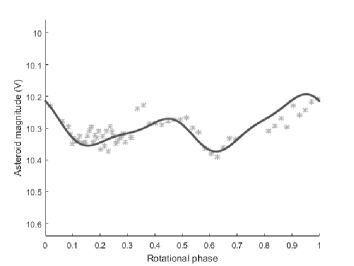
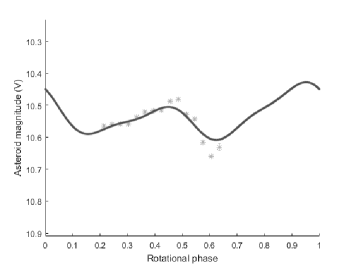
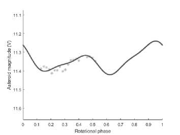
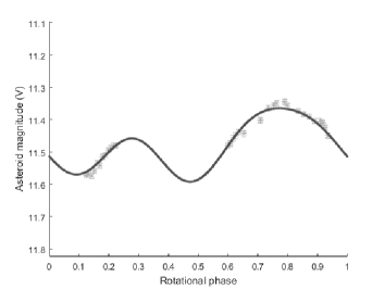
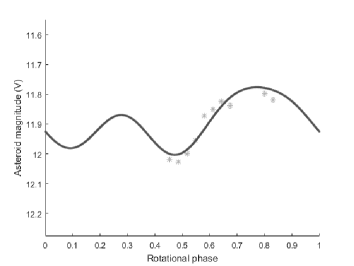
Figure 22: The two Fourier fit models for 85 Io superimposed on the observed data sessions (yyymmdd): 20121013, 20121015, 20121021, 20121116, 20121120, 20121206, from left to right, top to bottom.

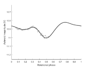
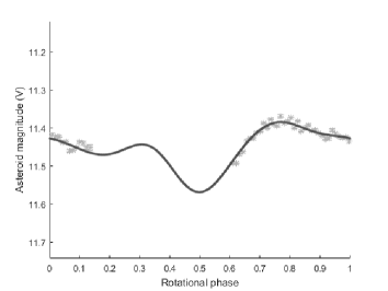
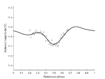
Figure 23: The Fourier fit model for 135 Herta superimposed on the observed data sessions (yyymmdd): 20121211, 20121219, 20121223, from left to right, top to bottom.

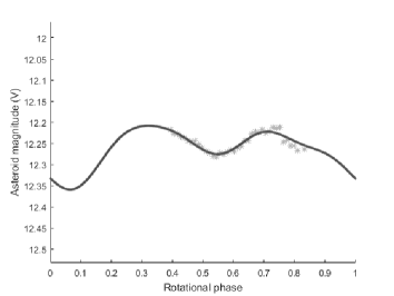
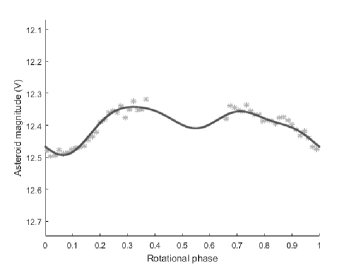
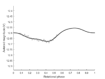
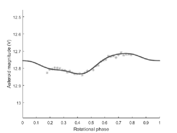
Figure 24: The three Fourier fit models for 313 Chaldea superimposed on the observed data sessions (yyymmdd): 20120920, 20120921, 20121002, 20121010, 20121015, 20121116, from left to right, top to bottom.

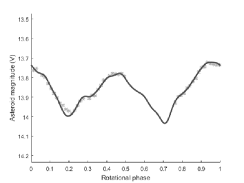
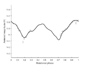
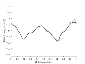
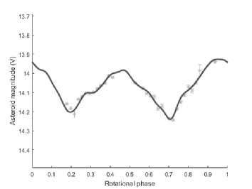
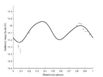
Figure 25: The two Fourier fit models for 522 Helga superimposed on the observed data sessions (yyymmdd): 20121002, 20121003, 20121010, 20121013, 20121021, 20121116, 20121206, from left to right, top to bottom.

Table 8: Summary of the lightcurve Fourier models with the reference Julian days - 2456000.5 and the fit orders used for each asteroids. In this table the asteroid 444 Gyptis is missing, it has not been analyzed because it is possible that it is a binary system.

Asteroids	$JD_{1}$	$n_{1}$	$JD_{2}$	$n_{2}$	$JD_{3}$	$n_{3}$
085 Io	214	4	253	3	-	-
135 Herta	280	5	-	-	-	-
208 Lacrimosa	264	5	-	-	-	-
236 Honoria	197	4	203	5	-	-
306 Unitas	255	5	-	-	-	-
308 Polyxo	306	5	-	-	-	-
313 Chaldaea	197	4	214	4	221	4
338 Budrosa	295	5	-	-	-	-
522 Helga	209	15	217	5	-	-
925 Alphonsina	318	5	-	-	-	-

Using several nights differential photometry data, we have construct a complete rotational lightcurve, with full coverage of the asteroid rotation. Once the full lightcurve and period have been determined, we created a Fourier fit with sufficient orders to capture all of the essential features of the lightcurve. Next we use the Fourier fit model of the full lightcurve as a way of extrapolating to data points that are not measured on a given night, i.e. the lightcurve maximum used for the phase curves. The best fit between data session and model was obtained by plotting the data on the Fourier curve and minimizing the squared error between the Fourier fit and the observed data, in this way the maximum brightness is determined with the contribution of the points of the whole session. In this appendix there are not all Fourier models but the selection shown is sufficient to understand what method has been adopted.

References

References

- Bowell et al. (1989) Bowell, E.G., Hapke, B., Domingue, D., Lumme, K., Peltoniemi, J., Harris, A.W. 1989. Application of photometric models to asteroids. In: Gehrels, T., Matthews, M.T., Binzel, R.P. (Eds.), Asteroids II. University of Arizona Press, pp. 524–555.
- Belskaya & Shevchenko (2000) Belskaya, I. N. & Shevchenko, V. G., 2000. Opposition Effect of Asteroids. Icarus 147, 94-105.
- Calcidese et al. (2012) Calcidese, P. Bernagozzi, A., Bertolini, E., Carbognani, A., Damasso, M., Pellissier, P., 2012. The Astronomical Observatory of the Autonomous Region of the Aosta Valley. A professional research centre in the Italian Alps. Mem. SAIt Supplement 19, 368-371.
- Cellino et al. (2016) Cellino, A., Bagnulo, S., Gil-Hutton, R., Tanga, P., Cañada-Assandri, M., and Tedesco, E.F., 2015. A polarimetric study of asteroids: fitting phase-polarization curves. MNRAS 455, 2091-2100.
- Cellino et al. (2015) Cellino, A., Bagnulo, S., Gil-Hutton, R., Tanga, P., Cañada-Assandri, M., and Tedesco, E.F., 2015. On the calibration of the relation between geometric albedo and polarimetric properties for the asteroids. MNRAS 451, 3473-3488.
- Cellino et al. (2009) Cellino, A., Hestroffer, D., Tanga, P., Mottola, S., & Dell’Oro, A., 2009. Genetic inversion of sparse disk.integrated photometric data of asteroids: application to Hipparcos data. A&A 506, 935-954.
- Devogèle et al. (2017) Devog‘ele, M., Cellino, A., Bagnulo, S., Rivet, J.-P., Bendjoya, Ph., Abe, L., Pernechele, C., Massone, G., Vernet, D., Tanga, P., Dimur, C., 2017. The Calern Asteroid Polarimetric Survey using the Torino polarimeter: assessment of instrument performances and first scientific results. MNRAS 465, 4335-4347.
- Dlugach and Mishchenko (2013) Dlugach, J. M. & Mishchenko, M. I., 2013. Coherent backscattering and opposition effects observed in some atmosphereless bodies of the solar system. Solar Syst. Res. 47, 454-462.
- Dunham et al. (2013) Dunham, D. W., Herald, D., Frappa, E., Hayamizu, T., Talbot, J., and Timerson, B., 2013. Asteroid Occultations V11.0. EAR-A-3-RDR-OCCULTATIONS-V11.0. NASA Planetary Data System, 2013.
- Gaia Collaboration (2018) The Gaia Collaboration, 2018. Gaia Data Release 2: Observations of solar system objects. A&A, in press, 2018.
- Gehrels (1956) Gehrels, T., 1956. Photometric Studies of Asteroids. V. The Light-Curve and Phase Function of 20 Massalia. Astrophysical Journal 123, 331-338.
- Harris et al. (1989b) Harris, A. W., Young, J. W., Contreiras, L., Dockweiler, T., Belkora, L., Salo, H., Harris, W. D., Bowell, E., Poutanen, M., Binzel, R. P., Tholen, D. J., Wang, S., 1989b. Phase Relations of High Albedo Asteroids. The unusual opposition brightening of 44 Nysa and 64 Angelina. Icarus 81, 365-374.
- Harris et al. (1989) Harris, A.W., Young, J.W., Bowell, E., Martin, L.J., Millis, R.L., Poutanen, M., Scaltriti, F., Zappala, V., Schober, H.J., Debehogne, H., Zeigler, K.W., 1989. Photoelectric Observations of Asteroids 3, 24, 60, 261, and 863. Icarus 77, 171-186
- Harris et al. (1981) Harris, W. E., Fitzgerald, M. & Cameron Reed, B., 1981. Photoelectric Photometry: an Approach to Data Reduction. Publications of the Astronomical Society of the Pacific 93, 507-517.
- Harris and Harris (1997) Harris, A. W., & Harris, A. W., 1997. On the Revision of Radiometric Albedos and Diameters of Asteroids. Icarus 126, 450-454.
- Masiero et al. (2011) Masiero, J. R., Mainzer, A. K., Grav, T., Bauer, J. M., Cutri, R. M., Dailey, J., Eisenhardt, P. R. M., McMillan, R. S., Spahr, T. B., Skrutskie, M. F., Tholen, D., Walker, R. G., Wright, E. L., DeBaun, E., Elsbury, D., Gautier IV, T., Gomillion, S., Wilkins, A., 2011. Main Belt asteroids with WISE/NEOWISE. I. Preliminary albedos and diameters. ApJ 741, 68.
- Muinonen et al. (2012) Muinonen, K., Mishchenko, M. I., Dlugach, J. M., Zubko, E., Penttilä, A. & Videen, G., 2012. Coherent Backscattering Verified Numerically for a Finite Volume of Spherical Particles. Ap.J. 760, Id 118.
- Muinonen et al. (2010) Muinonen, K., Belskaya, I. N., Cellino, A., Delb , M., Levasseur-Regourd, A. C., Penttil , A., Tedesco, E. F., 2010. A three-parameter magnitude phase function for asteroids. Icarus 209, 542-555.
- Muinonen (1994) Muinonen, K., 1994. Coherent Backscattering by Solar System Dust Particles. Asteroids, comets, meteors 1993 (A. Milani, M. Di Martino, A. Cellino, Eds.). International Astronomical Union Symposium no. 160, Kluwer Academic Publishers, Dordrecht, p.271.
- Penttilä et al. (2016) Penttilä, A., Shevchenko, V.G., Wilkman, O. & Muinonen, K., 2016. , , photometric phase function extended to low-accuracy data. Planet. space Sci. 123, 117-125.
- Pravec et al. (2012) Pravec, P., Harris, A. W., Ku nir k, P., Gal d, A., Hornoch, K., 2012. Absolute magnitudes of asteroids and a revision of asteroid albedo estimates from WISE thermal observations. Icarus 221, 365-387.
- Santana-Ros et al. (2015) Sanatana-Ros, T., Bartczak, P., Michalowski, T., Tanga, P., Cellino, A., 2015. Testing the inversion of asteroids’ Gaia photometry combined with ground-based observations. MNRAS 450, 333-341.
- Shevchenko (1997) Shevchenko, V. G., 1997. Analysis of Asteroid Brightness-Phase Relations. Solar System Research 31, 219-224.
- Shevchenko & Tedesco (2006) Shevchenko, V. G. & Tedesco, E. F., 2006. Asteroid albedos deduced from stellar occultation. Icarus 184, 211-220.
- Shevchenko et al. (2010) Shevchenko, V. G., Belskaya, I. N., Lupishko, D. F., Krugly, Yu. N., Chiorny, V. G., and Velichko, F. P., Eds., Kharkiv Asteroid Magnitude-Phase Relations V1.0. EAR-A-COMPIL-3-MAGPHASE-V1.0. NASA Planetary Data System, 2010.
- Shevchenko et al. (2016) Shevchenko, V. G., Belskaya, I. N., Muinonen, K., Penttilä, A., Krugly, Yu. N., Velichko, F. P., Chiorny, V. G., Slyusarev, I. G., Gaftonyuk, N. M., and Tereshenko, I. A., 2016. Asteroid observations at low phase angles. IV. Average parameters for the new , , magnitude system. Planet. Space Sci. 123, 101-116.
-
Warner et al. (2009)
Warner, B., Harris, A. W., Pravec, P., 2009. The asteroid lightcurve database. Icarus 202, 134-146.
http://www.MinorPlanet.info/lightcurvedatabase.html