Small field models of inflation
that predict a tensor-to-scalar ratio $r=0.03$

Abstract

Future observations of the cosmic microwave background (CMB) polarization are expected to set an improved upper bound on the tensor-to-scalar ratio of $r\lesssim 0.03$. Recently, we showed that small field models of inflation can produce a significant primordial gravitational wave signal. We constructed viable small field models that predict a value of $r$ as high as $0.01$. Models that predict higher values of $r$ are more tightly constrained and lead to larger field excursions. This leads to an increase in tuning of the potential parameters and requires higher levels of error control in the numerical analysis. Here, we present viable small field models which predict $r=0.03$. We further find the most likely candidate among these models which fit the most recent Planck data while predicting $r=0.03$. We thus demonstrate that this class of small field models is an alternative to the class of large field models. The BICEP3 experiment and the Euclid and SPHEREx missions are expected to provide experimental evidence to support or refute our predictions.

I Introduction

Improved measurements of the B-mode polarization of the cosmic microwave background (CMB) Seljak:1996ti ; Seljak:1996gy are expected to be more sensitive to the tensor-to-scalar ratio $r$. This ratio provides a measure of the amplitude of the primordial gravitational waves (GW), which in turn is a telltale of inflation Lyth:1996im . The final Planck data release and analysis Aghanim:2018eyx currently suggest an upper bound of $r<0.07$. The BICEP experiment Ade:2014xna ; Ade:2014gua ; Ade:2018gkx ; Barkats:2013jfa took data over the last few years Wu:2016hul which is expected to yield an upper bound of $r\leq 0.03$. A discovery of a value as high as $r\sim 0.03$ could indicate a very high energy scale $\sim 10^{16}GeV$ (see, for example, Lyth:1998xn ).

We continue our investigations Wolfson:2016vyx ; Wolfson:2018lel of a class of inflationary models that were proposed by Ben-Dayan and Brustein BenDayan:2009kv and were followed by Hotchkiss:2011gz ; Antusch:2014cpa ; Garcia-Bellido:2014wfa . This class of models is compatible with several fundamental physics considerations. Recently, interest in this class of models was revived by the discussion about the “swampland conjecture”, Lehners:2018vgi ; Garg:2018reu ; Kehagias:2018uem ; Ben-Dayan:2018mhe which suggests that small field models are favoured by various string-theoretical considerations (see Palti:2019pca for a recent review).

In addition, for this class of inflationary models, high values of $r$ result in a scale dependence of the scalar power spectrum. Future experiments such as Euclid Amendola:2012ys , and SPHEREx Dore:2014cca aim to probe the running of the scalar spectral index $\alpha$ at the level of $10\%$ relative error. This is a major improvement in comparison to the Planck bounds on $\alpha$ which are currently at the level of $\sim 75\%$ relative error. Such future measurements could provide additional constraints on our models.

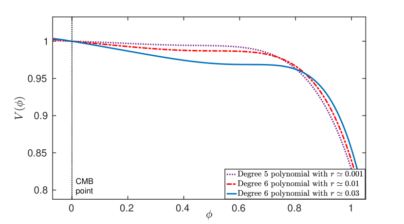
Figure 1: Polynomial potentials. The blue (solid) line depicts a potential of a model that predicts $r\simeq 0.03$, while the red (dash-dotted) line depicts a potential that predicts $r\simeq 0.01$. The purple (dotted) line depicts a degree five polynomial potential of a model that predicts $r\simeq 0.001$. All models are variants of the hilltop model, with a flatter region in which most e-folds are generated.

II The models

The small field models that we study are single-field models. The action of such models is given by

$$\mathcal{S}=\int d^{4}x\sqrt{-g}\left[\frac{R}{2}-\frac{1}{2}\partial^{\mu}\phi\partial_{\mu}\phi-V(\phi)\right].$$ (1)

The metric is of the FRW form and the potential given by

$$V(\phi)=V_{0}\left[1+\sum_{p=1}^{6}a_{p}\phi^{p}\right].$$ (2)

Previously, in BenDayan:2009kv ; Wolfson:2016vyx this class of models was discussed from a phenomenological and theoretical points of view. In Wolfson:2016vyx , the technical details of model building and simulation methods were discussed, while in Wolfson:2018lel , the analysis and the extraction of the most probable model were discussed. Additionally, in Wolfson:2018lel , the most likely model which yields $r=0.01$ was identified.

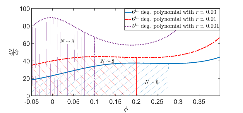
Figure 2: Field excursions in (reduced) Planck units. Different predicted values of $r$ require different field excursions to generate the $\sim 8$ e-folds probed by the CMB. The model predicting $r\simeq 0.03$ (blue line) requires an excursion of $\left(\Delta\phi\right)_{CMB}\simeq 0.28$ to generate the same amount of e-folds which the model predicting $r\simeq 0.01$ model (red dash-dot) generates in $\left(\Delta\phi\right)_{CMB}\simeq 0.2$. This means more tuning is required for models that predict $r\simeq 0.03$ . The model predicting $r\simeq 0.001$ (purple dots) requires only $\left(\Delta\phi\right)_{CMB}\simeq 0.1$ to generate the CMB window.

III Methods

We analyse the most recently available observational data Aghanim:2018eyx by using CosmoMC Lewis:2002ah , extracting the likelihood curves of the scalar index, its running and the running of running, $n_{s},\alpha,\beta$ respectively. We then simulate a large number of inflationary models with polynomial potentials and calculate the primordial power spectrum (PPS) observables $n_{s}$, $\alpha$, $\beta$, that they predict. Each simulated potential is assigned a likelihood by the combined likelihood of the observables that it yields, as discussed in detail in Wolfson:2018lel . We restrict the models that we consider to those predicting a power spectrum that can be fitted well by a third degree polynomial. This corresponds to the scalar index $n_{s}$, the index running $\alpha$, and the running of running $\beta$. We do that by fitting the PPS and evaluating the fitting error

$$\Delta^{2}=\frac{1}{n}\sum_{k=1}^{n}\left[\log(P_{S}(k))-f(k)\right]^{2},$$ (3)

where $f(k)$ is the fitting curve. The threshold for considering a specific model in our analysis is $\Delta^{2}<10^{-6}$.

An additional complication arises due to the higher amount of tuning that is required for these models. The coefficient $a_{1}$ is fixed as $a_{1}=-\sqrt{r/8}$ BenDayan:2009kv , so when the value of $r$ is higher, then $dV/d\phi$ at the CMB point has a larger magnitude. This has the effect of decreasing the number of e-folds generated per field excursion interval. If $r$ is increased to $Cr$, then $\frac{dN}{d\phi}$ is decreased by a factor $\sim\frac{1}{\sqrt{C}}$ close to the CMB point. Since the first 8 or so e-folds of inflation are fairly constrained by observations, the amount of freedom in constructing the potential is reduced. It follows that either greater tuning is required to construct valid potentials, or one should consider a higher degree polynomial as suggested in Hotchkiss:2011gz . Ultimately the choice is a matter of practical convenience. We opted for using sixth degree polynomials.

We employ two methods of retrieving the most likely polynomial potential. First, we extract by marginalisation the most likely coefficients $\{a_{p}\}$. The other method amounts to performing a multinomial fitting of the coefficients as a function of the observables and then inserting the most likely observables to recover the corresponding coefficients. This method is explained in detail in Wolfson:2018lel .

The ‘most likely model’, is the model with a potential that generates the most likely CMB observables $n_{S}\simeq 0.9687,\alpha\simeq 0.008,\beta\simeq 0.02$, as produced by the MCMC analysis of the most recent data available to date.

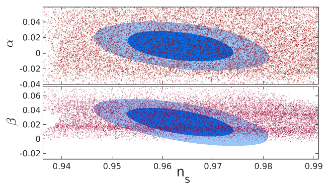
Figure 3: Covering the observable phase space with small field models that predict $r\simeq 0.03$. The roughly uniform cover of the $95\%$ CL areas ensures an accurate likelihood transfer from MCMC results to models.

IV Results

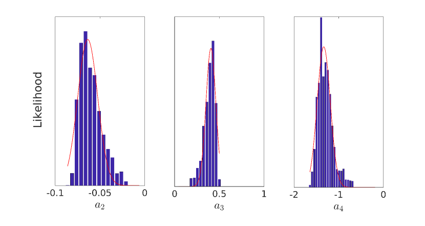
Figure 4: Likelihood analysis for model coefficients $a_{2},a_{3},a_{4}$, using Gaussian fits to recover mean values. The skewness of the results reflect properties of the model, not of the underlying MCMC analysis. The width of the Gaussian fits are given by $(0.016,0.08,0.21)$ and are an indication of the tuning level required for these models.

We produced many models that predict $r\simeq 0.03$ and, additionally, predict PPS observables within the likely values. A roughly uniform cover of both the $(n_{s},\alpha)$ and $(n_{s},\beta)$ allowed values is shown in Fig. 3. This enables us to assign likelihood to each simulated model, as discussed in detail in Wolfson:2016vyx ; Wolfson:2018lel . Consequently, it is possible to perform a likelihood analysis of models. The results of this likelihood analysis is an approximately Gaussian distribution of the free coefficients as is shown in Fig. 4. Since the peaks of Gaussian fit (red line in Fig. 4) do not quite coincide with the peaks of the distribution and the distribution tails are not symmetric, we conclude that the distribution has a significant skewness. The required tuning level is also evident from Fig. 4 and is given by $(\Delta a_{2},\Delta a_{3},\Delta a_{4})=(0.016,0.08,0.21)$. Using Gaussian analysis and taking into account the skewness, we recover the most likely coefficients, which yield the following degree six polynomial small field potential:

$$V=V_{0}\left[1-\sqrt{\frac{0.03}{8}}\phi-0.069\phi^{2}+0.431\phi^{3}-1.413\phi^{4}+2.455\phi^{5}-1.487\phi^{6}\right].$$ (4)

Due to the skewness of the distribution, the values obtained by the Gaussian fit deviate by a significant amount from the most likely values of the observables. For instance, $n_{s}$ as determined by the potential in (4) is $\sim 0.98$ which is about $2\%$ away from the most likely value. For this reason we use this method of analysis to evaluate the required tuning levels, whereas the most likely model is extracted by the multinomial fitting method.

Using the popular Stewart-Lyth (SL) theoretical values for $n_{s}$ and $\alpha$ Stewart:1993bc ; Lyth:1998xn as derived directly from the inflationary potential around the pivot scale, one finds values that deviate by a large amount from the Planck values. The SL values correspond to a very blue power spectrum and large running,

$$\left.n_{s}\right|_{SL}\simeq 1.55$$ (5)

$$\left.\alpha\right|_{SL}\simeq-0.216.$$

This discrepancy, that was discussed in Wolfson:2016vyx , is related to the magnitude of $r$ for our class of models. When $r$ is smaller than $\sim 10^{-4}$ in such models, the original model building procedure that relied on the SL values, which is outlined in BenDayan:2009kv , is valid and produces approximately the correct values of the observables. However, when values of $r$ are larger, one cannot trust the analytic SL estimates.

In Fig. 5 the power spectra generated by three inflationary models are shown. (1) A model with degree five polynomial potential that predicts $r\simeq 0.001$; (2) A model with degree six polynomial potential that predicts $r\simeq 0.01$; and finally (3) A model with degree six polynomial potential that predicts $r\simeq 0.03$.

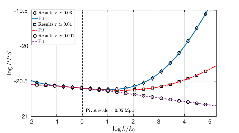
Figure 5: Primordial power spectra of three models. A model with a degree six polynomial potential that predicts $r\simeq 0.03$ (diamonds and blue line). A model with a degree six polynomial potential that predicts $r\simeq 0.01$ (squares and red dash-dot) and a model with a degree five polynomial potential that predicts $r=0.001$ (circles and purple dots). The pivot scale for all three is $k_{0}=0.05\mathrm{Mpc^{-1}}$ and the results are overlayed at that scale for ease of comparison.

Representing each coefficient $a_{p}$ as a function of the observables $(n_{s},\alpha,\beta)$ and evaluating them at $(0.9687,0.008,0.02)$, leads to the following potential,

$$V=V_{0}\left[1-\sqrt{\frac{0.03}{8}}\phi-0.067\phi^{2}+0.413\phi^{3}-1.419\phi^{4}+2.512\phi^{5}-1.523\phi^{6}\right].$$ (6)

The values $n_{s},\alpha,\beta$ that this model predicts deviate from the most likely values by $(0.06\%,10\%,19\%)$. However, the deviations are within the $95\%$ CL of all recent MCMC analyses.

V Conclusion

We presented and discussed small field models of inflation with a degree six polynomial potential that predict $r\simeq 0.03$. The most likely of these models also predicts the most likely values of $n_{s},\alpha,\beta$, within currently acceptable margins of error. The amount of coefficient tuning for these models was calculated. This article, along with its predecessors Wolfson:2016vyx ; Wolfson:2018lel , demonstrates that an interesting range of values of $r$, $0.001\leq r\leq 0.03$ can be predicted by small field models of inflation that are consistent with the available CMB data.

- (1) U. Seljak, “Measuring polarization in cosmic microwave background,” Astrophys. J. 482 (1997) 6 [astro-ph/9608131].
- (2) U. Seljak and M. Zaldarriaga, “Signature of gravity waves in polarization of the microwave background,” Phys. Rev. Lett. 78 (1997) 2054 [astro-ph/9609169].
- (3) Lyth D. H., “What would we learn by detecting a gravitational wave signal in the cosmic microwave background anisotropy?,” Phys. Rev. Lett. 78 (1997) 1861 [hep-ph/9606387].
- (4) N. Aghanim et al. [Planck Collaboration], “Planck 2018 results. VI. Cosmological parameters,” arXiv:1807.06209 [astro-ph.CO].
- (5) P. A. R. Ade et al. [BICEP2 Collaboration], “Detection of -Mode Polarization at Degree Angular Scales by BICEP2,” Phys. Rev. Lett. 112 (2014) no.24, 241101 [arXiv:1403.3985 [astro-ph.CO]].
- (6) P. A. R. Ade et al. [BICEP2 Collaboration], “BICEP2 II: Experiment and Three-Year Data Set,” Astrophys. J. 792 (2014) no.1, 62 [arXiv:1403.4302 [astro-ph.CO]].
- (7) P. A. R. Ade et al. [BICEP2 and Keck Array Collaborations], “BICEP2 / Keck Array x: Constraints on Primordial Gravitational Waves using Planck, WMAP, and New BICEP2/Keck Observations through the 2015 Season,” Phys. Rev. Lett. 121, 221301 (2018) [arXiv:1810.05216 [astro-ph.CO]].
- (8) D. Barkats et al. [BICEP1 Collaboration], “Degree-Scale CMB Polarization Measurements from Three Years of BICEP1 Data,” Astrophys. J. 783 (2014) 67 [arXiv:1310.1422 [astro-ph.CO]].
- (9) W. L. K. Wu et al., “Initial Performance of BICEP3: A Degree Angular Scale 95 GHz Band Polarimeter,” J. Low. Temp. Phys. 184 (2016) no.3-4, 765 [arXiv:1601.00125 [astro-ph.IM]].
- (10) D. H. Lyth and A. Riotto, “Particle physics models of inflation and the cosmological density perturbation,” Phys. Rept. 314, 1 (1999) [hep-ph/9807278].
- (11) I. Wolfson and R. Brustein, “Small field models with gravitational wave signature supported by CMB data,” PLoS One 13 (2018) 1 [arXiv:1607.03740 [astro-ph.CO]].
- (12) I. Wolfson and R. Brustein, “Most probable small field inflationary potentials,” arXiv:1801.07057 [astro-ph.CO].
- (13) I. Ben-Dayan and R. Brustein, “Cosmic Microwave Background Observables of Small Field Models of Inflation,” JCAP 1009 (2010) 007 [arXiv:0907.2384 [astro-ph.CO]].
- (14) S. Hotchkiss, A. Mazumdar and S. Nadathur, “Observable gravitational waves from inflation with small field excursions,” JCAP 1202, 008 (2012) [arXiv:1110.5389 [astro-ph.CO]].
- (15) S. Antusch and D. Nolde, “BICEP2 implications for single-field slow-roll inflation revisited,” JCAP 1405, 035 (2014) [arXiv:1404.1821 [hep-ph]].
- (16) J. Garcia-Bellido, D. Roest, M. Scalisi and I. Zavala, “Lyth bound of inflation with a tilt,” Phys. Rev. D 90, no. 12, 123539 (2014) [arXiv:1408.6839 [hep-th]].
- (17) J. L. Lehners, “Small-Field and Scale-Free: Inflation and Ekpyrosis at their Extremes,” JCAP 1811 (2018) no.11, 001 [arXiv:1807.05240 [hep-th]].
- (18) S. K. Garg and C. Krishnan, “Bounds on Slow Roll and the de Sitter Swampland,” arXiv:1807.05193 [hep-th].
- (19) A. Kehagias and A. Riotto, “A note on Inflation and the Swampland,” Fortsch. Phys. 66 (2018) no.10, 1800052 [arXiv:1807.05445 [hep-th]].
- (20) I. Ben-Dayan, “Draining the Swampland,” arXiv:1808.01615 [hep-th].
- (21) E. Palti, “The Swampland: Introduction and Review,” arXiv:1903.06239 [hep-th].
- (22) L. Amendola et al. [Euclid Theory Working Group], “Cosmology and fundamental physics with the Euclid satellite,” Living Rev. Rel. 16 (2013) 6 [arXiv:1206.1225 [astro-ph.CO]].
- (23) O. Doré et al., “Cosmology with the SPHEREX All-Sky Spectral Survey,” arXiv:1412.4872 [astro-ph.CO].
- (24) A. Lewis and S. Bridle, “Cosmological parameters from CMB and other data: A Monte Carlo approach,” Phys. Rev. D 66 (2002) 103511 [astro-ph/0205436].
- (25) E. D. Stewart and D. H. Lyth, “A More accurate analytic calculation of the spectrum of cosmological perturbations produced during inflation,” Phys. Lett. B 302 (1993) 171 [gr-qc/9302019].