Achronal ANEC, Weak Cosmic Censorship, and AdS/CFT duality

Abstract

We examine the achronal averaged null energy condition (ANEC) for a class of conformal field theories (CFT) at strong coupling in curved spacetime. By applying the AdS/CFT duality, we find holographic models which violate the achronal ANEC for $3+1$ and $4+1$-dimensional boundary theories. In our model, the bulk spacetime is an asymptotically AdS vacuum bubble solution with neither causality violation nor singularities. The conformal boundary of our bubble solution is asymptotically flat and is causally proper in the sense that a “fastest null geodesics” connecting any two points on the boundary must lie entirely on the boundary. We show that conversely, if the spacetime fails to have this causally proper nature, then there must be a naked singularity in the bulk.

I Introduction

The classical null energy condition (NEC) $T_{\mu\nu}l^{\mu}l^{\nu}\geq 0$ for all null vectors $l$ at all points is the key condition for the proof of the singularity theorems, topological censorship theorem, and other important theorems in classical general relativity. Although it is satisfied for typical classical matter fields, the NEC can be violated when one considers quantum field effects. For example, when one spatial dimension is compactified, $\left\langle~{}T_{\mu\nu}~{}\right\rangle l^{\mu}l^{\nu}$ becomes negative along the null geodesic of the closed $S^{1}$ circle, where $\left\langle~{}T_{\mu\nu}~{}\right\rangle$ is the vacuum expectation value of the stress-energy tensor. In general, any locally formulated energy conditions can be violated by quantum field effects.

The averaged null energy condition (ANEC) is an alternative condition which is non-locally formulated and states that

$$\int^{\infty}_{-\infty}\left\langle~{}T_{\mu\nu}~{}\right\rangle l^{\mu}l^{\nu}d\lambda\geq 0\,,$$ (1)

for every complete null geodesic with tangent vector $l^{\mu}$, where $\lambda$ is the affine parameter. It has been shown that the ANEC is satisfied for some cases, e.g., minimally coupled scalar fields in Minkowski spacetime Klinkhammer1990 ; WaldYurtsever1991 in $4$-dimensions and in curved spacetime Yurtsever1990 ; WaldYurtsever1991 in 2-dimensions. For further examples in which the ANEC holds, see Refs. Ford_Roman1995 ; Yurtsever1995 . However, it has been shown that for a conformally coupled scalar field, the ANEC can be violated for any chronal null geodesics in Schwarzschild spacetime Visser1996 . This example of ANEC violation has led Graham and Olum GrahamOlum to propose the achronal ANEC, which states that the ANEC should hold for every complete achronal null geodesic but not necessarily on chronal null geodesics. Here, an achronal null geodesic refers to a null geodesic curve on which no two points can be connected by a timelike curve. A complete achronal null geodesic is also called a null line. Further studies, however, revealed cases in which the achronal ANEC can also be violated Visser1995 ; UrbanOlum . This fact suggests the possibility of, e.g., the formation of exotic objects such as wormholes, since the achronal ANEC is crucial for the proof of singularity theorems and topological censorship.

It is interesting to study whether the achronal ANEC is violated in a strongly coupled field theory in the framework of the AdS/CFT duality. In this context it was recently shown in KellyWall2014 that the achronal ANEC holds for a class of conformal field theories in the boundary Minkowski spacetime. This is consistent with the numerical verification of the achronal ANEC for colliding planar shock wave solutions derSchee2014 .

Applying the AdS/CFT duality, an example of NEC violation in curved space was recently found in IMM2018 , in which the gravity dual is a vacuum AdS black hole solution, and the boundary spacetime describes a wormhole geometry which connects two asymptotically flat universes. In this example, as the bulk solution asymptotically approaches the planar Schwarzschild-AdS solution, the corresponding boundary thermal states render $\left\langle~{}T_{\mu\nu}~{}\right\rangle l^{\mu}l^{\nu}$ strictly positive in the asymptotic region of the boundary spacetime. Therefore even though the NEC is locally violated near the wormhole throat, the achronal ANEC is kept preserved. This suggests that the achronal ANEC may always hold in a thermal state with asymptotically flat boundary spacetime.

In this paper, we further examine the achronal ANEC for a class of strongly coupled field theories in asymptotically flat curved spacetimes in the framework of the AdS/CFT duality. If and when there exists a timelike curve in the bulk that connects two points on a boundary achronal null geodesic, one can say that the corresponding boundary theory admits an acausal signal. We shall reveal some possible relations between the achronal ANEC, weak cosmic censorship, and acausal propagation of signals, provide some examples of an achronal ANEC violation without acausal signals and finally discuss what happens when there are acausal signals.

We first give examples of a violation of the achronal ANEC in $d=4$ and $5$ boundary spacetimes with respectively, $d+1=5$ and $6$ bulk solutions of the vacuum Einstein equations with a negative cosmological constant. Our strategy is similar to Ref. UrbanOlum . In the case of $d=4$, we start with a vacuum bubble AdS solution, also called the AdS soliton, as our 5-dimensional bulk spacetime. We show that a certain choice of conformal factor for a conformally flat, $d=4$ boundary spacetime induces a gravitational conformal anomaly HaroSkenderis , which leads to the violation of the achronal ANEC. For $d=5$ spacetimes, there is no gravitational anomaly. We construct a regular $6$-dimensional bulk vacuum bubble solution with a curved $d=5$ boundary spacetime. The resulting boundary stress-energy tensor shows that the NEC on the boundary is violated but the ANEC on the boundary still holds. Then, by choosing a suitable conformal factor, we show that the achronal ANEC in the conformally transformed system can be violated.

It is worth mentioning that both of our two examples are “causally proper” in the sense that there is no bulk timelike curve that could connect any two points on each achronal null geodesic on the boundary, implying a “fastest null geodesics” connecting any two points on the boundary must lie entirely on the boundary. In addition, there is no pathological behavior in the boundary spacetime: it is in fact geodesically complete and asymptotically flat. It is then interesting to consider what would possibly happen if, on the other hand, the causally proper nature is not satisfied. We will show by using the Gao-Wald theorem GaoWald that if the geometry under consideration fails to be causally proper while preserving the NEC in the bulk, then there must appear a naked singularity; the weak cosmic censorship must fail.

In the next section we consider the achronal ANEC in $d=4$ boundary theory. In Sec. III, we construct a $6$-dimensional perturbed bubble solution which leads to the violation of the ANEC. A proposition which connects the bulk cosmic censorship and the causally proper nature is presented in Sec. IV. Sec. V is devoted to summary and discussions.

II Violation of achronal ANEC in even dimensions

In this section, we explore the ANEC in a $5$-dimensional holographic model. In $d$-dimensional boundary theory with $d$ even, the bulk metric is expressed in the Fefferman-Graham coordinate system:

$$ds^{2}=\frac{1}{z^{2}}\left[dz^{2}+\Bigl{(}\sum_{n=0}^{\infty}g_{(n)\mu\nu}z^{n}+z^{d}\ln z^{2}h_{\mu\nu}\Bigr{)}dx^{\mu}dx^{\nu}\right]$$ (2)

with the boundary metric $ds_{\partial}^{2}=g_{(0)\mu\nu}dx^{\mu}dx^{\nu}$ located at $z=0$ HaroSkenderis . Here, the logarithmic term only appears for even dimensions, and $g_{(2k+1)\mu\nu}=0$ for any integer $k$ satisfying $0\leq 2k+1<d$. The holographic stress-energy tensor $\left\langle~{}T_{\mu\nu}~{}\right\rangle$ includes conformal anomalies, and it is given by

$$\left\langle~{}T_{\mu\nu}~{}\right\rangle=g_{(4)\mu\nu}-\frac{1}{8}g_{(0)\mu\nu}\left\{(g^{\alpha}_{(2)\alpha})^{2}-g^{\alpha}_{(2)\beta}g^{\beta}_{(2)\alpha}\right\}$$

$$\quad\quad\quad\quad-\frac{1}{2}g_{(2)\mu\alpha}g^{\alpha}_{(2)\nu}+\frac{1}{4}g_{(2)\mu\nu}g^{\alpha}_{(2)\alpha},$$ (3)

where the gravitational constant $G_{4}$ is set to be $4\pi G_{4}=1$ and the index is raised and lowered by the boundary metric $g_{(0)\mu\nu}$. The coefficient $g_{(2)}$ is induced by the Ricci tensor on the boundary metric $ds_{\partial}^{2}$ HaroSkenderis , so we consider a conformal transformation of the boundary metric $d\hat{s}_{\partial}^{2}=a(x^{\mu})^{2}ds_{\partial}^{2}$ and investigate whether the achronal ANEC can be violated for the boundary conformal field theory. Note that in a conformally flat spacetime, any null geodesics are achronal. We are interested in the boundary metric where the null geodesics are complete in both future and past directions and the l. h. s. of Eq. (1) converges. We consider a conformal factor $a(x^{\mu})$ satisfying the following conditions;

Condition A

1. $a(\lambda)$ is everywhere regular (at least twice differentiable) and positive-definite.

2. At $\lambda\rightarrow\pm\infty$, $a(\lambda)$ approaches some finite positive constant values.

where $\lambda$ is the affine parameter of the null geodesic.

II.1 Achronal ANEC for a simple case

We start with a 5-dimensional vacuum bubble solution with the metric,

$$ds^{2}=\left(r^{2}-\frac{r_{0}^{4}}{r^{2}}\right)d\chi^{2}+\frac{dr^{2}}{\left(r^{2}-\frac{r_{0}^{4}}{r^{2}}\right)}+r^{2}(dx^{2}+dy^{2}-dt^{2}),$$ (4)

where $\chi\in[0,\,\pi/r_{0}]$, and the (conformal) boundary metric is $ds_{\partial}^{2}=-dt^{2}+dx^{2}+dy^{2}+d\chi^{2}$. A good place to start is to consider first the case where $a$ depends on $x$ only. As done in the cosmological case Siopsis2009 , one needs to make a change of coordinates $(r,\,x)\to(z,\,\rho)$ to bring (4) to the Fefferman-Graham coordinate (2) with the boundary metric $d\hat{s}_{\partial}^{2}=a(x)^{2}ds_{\partial}^{2}$.

Introducing new coordinates $z$ and $\rho$ as

$$\frac{1}{r}=z\left(\frac{1}{a(x)}+\alpha_{1}(x)z^{2}+\alpha_{2}(x)z^{4}+\cdots\right),$$

$$x(\rho,\,z)=\rho+\beta_{1}(\rho)z^{2}+\beta_{2}(\rho)z^{4}+\cdots,$$

$$a(x)=a(\rho)+a^{\prime}(\rho)\beta_{1}(\rho)z^{2}+\Bigl{(}a^{\prime}(\rho)\beta_{2}(\rho)$$

$$\quad\quad\quad+\frac{1}{2}\beta_{1}^{2}(\rho)a^{\prime\prime}(\rho)\Bigr{)}z^{4}+\cdots,$$ (5)

the bubble metric (4) is reduced to the Fefferman-Graham metric (2) under the conditions

$$\alpha_{1}(\rho)=-a(\rho)\beta_{1}^{2}(\rho),\;\;\alpha_{2}(\rho)=\frac{a^{\prime}(\rho)^{4}-2r_{0}^{4}\,a(\rho)^{4}}{16a(\rho)^{9}},$$

$$\beta_{1}(\rho)=\frac{a^{\prime}(\rho)}{2a(\rho)^{3}},\quad\beta_{2}(\rho)=-\frac{a^{\prime}(\rho)^{3}}{8a(\rho)^{7}},\cdots,$$ (6)

where $a^{\prime}=\partial_{\rho}a$. For our purpose, the other higher order coefficients are not needed, as we are only concerned with the derivation of Eq. (II). The coordinate transformation just corresponds to choosing a different foliation from the original bubble solution (4).

Each coefficient in the Fefferman-Graham metric is given by

$$g^{(0)}_{\mu\nu}dx^{\mu}dx^{\nu}=a(\rho)^{2}(-dt^{2}+d\rho^{2}+dy^{2}+d\chi^{2}),$$

$$g^{(2)}_{\mu\nu}dx^{\mu}dx^{\nu}=-\frac{a^{\prime}(\rho)^{2}}{2a(\rho)^{2}}dt^{2}$$

$$+\frac{2a(\rho)a^{\prime\prime}(\rho)-3a^{\prime}(\rho)^{2}}{2a(\rho)^{2}}d\rho^{2}+\frac{a^{\prime}(\rho)^{2}}{2a(\rho)^{2}}(dy^{2}+d\chi^{2}),$$

$$g^{(4)}_{\mu\nu}dx^{\mu}dx^{\nu}=\frac{4r_{0}^{4}\,a(\rho)^{4}+a^{\prime}(\rho)^{4}}{16a(\rho)^{6}}(-dt^{2}+dy^{2})$$

$$+\frac{-12r_{0}^{4}\,a(\rho)^{4}+a^{\prime}(\rho)^{4}}{16a(\rho)^{6}}d\chi^{2}+d\rho^{2}\frac{1}{16a(\rho)^{6}}\times$$

$$\biggl{\{}9a^{\prime}(\rho)^{4}+4a(\rho)[r_{0}^{4}\,a(\rho)^{3}-3a^{\prime}(\rho)^{2}a^{\prime\prime}(\rho)+a(\rho)a^{\prime\prime}(\rho)^{2}]\biggr{\}}.$$ (7)

Substituting the above coefficients into Eq. (II), one obtains

$$\left\langle~{}T_{tt}~{}\right\rangle=-\frac{4r_{0}^{4}\,a(\rho)^{4}+5a^{\prime}(\rho)^{4}-4a(\rho)a^{\prime}(\rho)^{2}a^{\prime\prime}(\rho)}{16a(\rho)^{6}},$$

$$\left\langle~{}T_{\rho\rho}~{}\right\rangle=\frac{4r_{0}^{4}\,a(\rho)^{4}-3a^{\prime}(\rho)^{4}}{16a(\rho)^{6}},$$

$$\left\langle~{}T_{yy}~{}\right\rangle=\frac{4r_{0}^{4}\,a(\rho)^{4}+5a^{\prime}(\rho)^{4}-4a(\rho)a^{\prime}(\rho)^{2}a^{\prime\prime}(\rho)}{16a(\rho)^{6}},$$

$$\left\langle~{}T_{\chi\chi}~{}\right\rangle=-\frac{12r_{0}^{4}\,a(\rho)^{4}-5a^{\prime}(\rho)^{4}+4a(\rho)a^{\prime}(\rho)^{2}a^{\prime\prime}(\rho)}{16a(\rho)^{6}}.$$ (8)

Note that $\left\langle~{}{T^{\mu}}_{\mu}~{}\right\rangle\neq 0$ unless $a(\rho)$ is constant. This is the effect of the conformal anomaly, which appears only for even dimensions. Now consider the null geodesic generator

$$\hat{l}=\frac{1}{a^{2}(x)}(\partial_{t}+\partial_{x})$$ (9)

on the conformal boundary. Since the boundary metric is conformally flat, and the null geodesic orbit does not change for any conformal transformation, the null geodesic curve generated by $\hat{l}$ is achronal on the boundary theory.

Under the condition A, the l. h. s. of Eq. (1) is evaluated as

$$I=\int^{\infty}_{-\infty}T_{\mu\nu}\hat{l}^{\mu}\,\hat{l}^{\nu}\,d\lambda$$

$$=\int^{\infty}_{-\infty}\frac{a(\rho)a^{\prime}(\rho)^{2}a^{\prime\prime}(\rho)-2a^{\prime}(\rho)^{4}}{4a(\rho)^{8}}d\rho$$

$$=\int^{\infty}_{-\infty}\frac{a^{\prime}(\rho)^{4}}{12a(\rho)^{8}}d\rho\geq 0,$$ (10)

where we used condition A to derive the last equality by integration by parts. This means that the achronal ANEC is satisfied for any conformal factor $a(\rho)$ satisfying the asymptotic boundary condition A.

II.2 Violation of achronal ANEC for a generic scale factor $a$

In this subsection we consider the case of generic scale factor $a(t,x,y)$, which depends on $t$, $x$, and $y$. Introducing new coordinates $\hat{x}^{\mu}~{}(\mu=0,1,2)$ and $z$ as

$$\frac{1}{r}=z\left(\frac{1}{a(x)}+\alpha_{1}(x)z^{2}+\alpha_{2}(x)z^{4}+\cdots\right),$$

$$x^{\mu}(\hat{x},\,z)=\hat{x}^{\mu}+\beta_{1}^{\mu}(\hat{x})z^{2}+\beta_{2}^{\mu}(\hat{x})z^{4}+\cdots,$$ (11)

we obtain the Fefferman-Graham metric (2) under the conditions

$$\beta_{1}^{\mu}=\frac{\nabla^{\mu}a}{2a^{3}},\qquad\beta_{2}^{\mu}=-\frac{\nabla^{\mu}a(\nabla a)^{2}}{8a^{7}},$$

$$\alpha_{1}=-\frac{(\nabla a)^{2}}{4a^{5}},\qquad\alpha_{2}=\frac{-2r_{0}^{4}\,a^{4}+((\nabla a)^{2})^{2}}{16a^{9}},\cdots,$$ (12)

where $\nabla$ is the covariant derivative with respect to the metric $ds^{2}=-dt^{2}+dx^{2}+dy^{2}$, and $(\nabla a)^{2}=\nabla_{\mu}a\nabla^{\mu}a$.

Now, let us define $a=e^{\omega}$ and suppose $|\omega|\ll 1$. Then, the null-null component of the stress-energy tensor becomes

$$\left\langle~{}T_{\mu\nu}~{}\right\rangle\hat{l}^{\mu}\hat{l}^{\nu}\simeq$$

$$\frac{1}{4}\Bigl{[}-(\omega_{,yt}+\omega_{,xy})^{2}+\omega_{,yy}(\omega_{,tt}+2\omega_{,xt}+\omega_{,xx})\Bigr{]}+O(\omega^{3}).$$ (13)

As an example, if one takes $\omega$ as

$$\omega=\epsilon e^{-(t^{2}+x^{2}+y^{2})},$$ (14)

with $\epsilon\ll 1$, we obtain

$$\left\langle~{}T_{\mu\nu}~{}\right\rangle\hat{l}^{\mu}\hat{l}^{\nu}$$

$$=-2\epsilon^{2}e^{-2(t^{2}+x^{2}+y^{2})}\{(t+x)^{2}+2y^{2}-1\}+O(\epsilon^{3}).$$ (15)

It is easily checked that there exist null lines which can violate the ANEC. For instance, consider the curve $y=1$, $x=t$. For this, the l. h. s. of Eq. (1) yields a negative value as

$$\int^{\infty}_{-\infty}\left\langle~{}T_{\mu\nu}~{}\right\rangle\hat{l}^{\mu}\hat{l}^{\nu}d\lambda\simeq-\frac{3\sqrt{\pi}}{2e^{2}}\epsilon^{2}<0,$$ (16)

So, the ANEC is violated. The situation is very similar to the case of conformally coupled scalar field in a conformally flat spacetime UrbanOlum .

It is easily checked by the bubble metric (4) that the bulk spacetime is causally proper because the tangent vector $k:=\partial_{t}+C_{1}\partial_{x}+C_{2}\partial_{r}$ on the bulk causal curve $\gamma$ satisfies $C_{1}\leq 1$ and the equality holds only for the boundary null geodesic with $C_{2}=0$.

III Violation of achronal ANEC in odd-dimensions

In the previous section, we have shown that the achronal ANEC can be violated in the boundary CFT theory with even dimension, due to the conformal anomaly. When $d$ is odd, the conformal anomaly terms disappear and the stress-energy tensor becomes just the coefficientHaroSkenderis

$$\left\langle~{}T_{\mu\nu}~{}\right\rangle=\frac{d}{16\pi G_{d}}g_{(d)\mu\nu}$$ (17)

in the Fefferman-Graham coordinate system (2). The stress-energy tensor is conformally covariant under the conformal transformation $d\hat{s}_{\partial}^{2}=a^{2}ds_{\partial}^{2}$, just being conformally rescaled with no additive terms. Therefore, unless the NEC is violated (i.e., $\left\langle~{}T_{\mu\nu}~{}\right\rangle$ is negative at some point on the boundary), the achronal ANEC cannot be violated (subject to condition A on the conformal factor). In what follows, we set ${d}/{16\pi G_{d}}=1$, for simplicity.

We start with the following 6-dimensional bubble solutions

$$ds^{2}=\frac{4}{25r_{0}^{2}}\left(r^{2}-\frac{r_{0}^{5}}{r^{3}}\right)d\chi^{2}+\frac{dr^{2}}{r^{2}-{r_{0}^{5}}/{r^{3}}}$$

$$+r^{2}(dx^{2}+dy^{2}+dw^{2}-dt^{2})\,.$$ (18)

where $r\in[r_{0},\,\infty]$ and $\chi\in[0,\,2\pi]$. The stress-energy tensor (17) contracted by the null vector $n=\partial_{t}+(5r_{0}/2)\partial_{\chi}$ becomes negative (see Appendix for $\epsilon=0$),

$$\left\langle~{}T_{\mu\nu}~{}\right\rangle n^{\mu}n^{\nu}=-r_{0}^{2}<0.$$ (19)

Although the ANEC (1) is violated along the $S^{1}$ circle, this does not mean that the achronal ANEC is also violated because the closed orbit is not achronal. On the other hand, along the null line with null tangent vector $l=\partial_{t}+\partial_{x}$,

$$\left\langle~{}T_{\mu\nu}~{}\right\rangle l^{\mu}l^{\nu}=0.$$ (20)

This suggests that the perturbation of the bubble spacetime (III) could induce a non-zero stress-energy tensor which locally violates the NEC along the achronal null geodesic and hence potentially lead to ANEC violation. We note that one may desire instead to consider a perturbation of the Poincare AdS solution $(r_{0}=0)$ rather than the bubble solution, since it is much simpler and Eq. (20) is still satisfied. In that case, however, $pp$-type curvature singularities are generally expected to occur on the horizon for generic perturbations ChamblinGibbons . On the other hand, one expects the bubble spacetime to be stable Horowitz:1998ha In the next subsection, we consider the perturbation of the bubble solution (III).

III.1 The perturbed variables

Let us consider the slightly deformed bubble solution by additing to (III) the following static metric perturbations:

$$\delta g_{\mu\nu}=2\epsilon r^{2}(H\eta_{\mu\nu}S+H_{T}S_{\mu\nu}),\quad\delta g_{\chi\chi}=\epsilon f_{\chi\chi}S\,,$$ (21)

where $\epsilon$ is a small positive parameter and the Greek indices $\mu,\nu,\dots$ denote the specific choice of coordinates $x,\,y,\,w,\,t$ used in (III). Here, $f_{\chi\chi},\>H,\>H_{T}$ are functions of $r$, and $S$, $S_{\mu}$, and $S_{\mu\nu}$ are defined in terms of $\rho=\sqrt{x^{2}+y^{2}+w^{2}}$ and a real positive parameter $k$ by

$$S=\frac{\sin k\rho}{\rho}\,,$$

$$S_{\mu}=-\frac{1}{k}D_{\mu}S,\quad S_{\mu\nu}=\frac{1}{k^{2}}D_{\mu}D_{\nu}S+\frac{1}{4}\eta_{\mu\nu}S\,,$$ (22)

with the covariant derivative operator $D_{\mu}$ associated with $\eta_{\mu\nu}$. Note that $S$ is regular at $\rho=0$ and $\lim_{\rho\rightarrow\infty}S=0$, guaranteeing the asymptotic convergence of the l. h. s. of Eq. (1), as we will show later. Note also that $S$ satisfies

$$D_{\mu}D^{\mu}S+k^{2}S=0\,,$$ (23)

where one may view the above deformation (21) as the Wick-rotated version of a restricted class of the scalar-type metric perturbations of the 6-dimensional Schwarzschild-AdS metric. Then, following the formulae of Kodama_Ishibashi2003 , one can derive the equations that determine the three perturbation variables $f_{\chi\chi},H,H_{T}$:

$$(r^{6}-r_{0}^{5}\,r)g^{\prime\prime}(r)+\left(7r^{5}+\frac{r_{0}^{5}}{2}\right)g^{\prime}(r)$$

$$\quad\quad\quad\quad-k^{2}r^{2}g(r)+4(2r^{5}+3r_{0}^{5})H^{\prime}(r)=0,$$

$$(r^{6}-r_{0}^{5}\,r)H^{\prime\prime}(r)+2(r^{5}-r_{0}^{5})H^{\prime}(r)$$

$$\quad\quad\quad\quad\quad-\frac{1}{2}(r^{5}-r_{0}^{5})g^{\prime}(r)+\frac{k^{2}r^{2}}{8}g(r)=0,$$ (24)

with

$$H_{T}(r)=\frac{8}{3k^{2}r^{2}}\left(8r^{5}-3r_{0}^{5}\right)H^{\prime}(r)-4H(r)$$

$$\quad\quad\quad+\frac{8}{3k^{2}r^{2}}\left(r^{5}-r_{0}^{5}\right)g^{\prime}(r)-\frac{2}{3}g(r),$$ (25)

where $g$ is defined as

$$f_{\chi\chi}=\frac{4}{25r_{0}^{2}}\left(r^{2}-\frac{r_{0}^{5}}{r^{3}}\right)g(r)\,.$$ (26)

Let us expand the functions $H$ and $g$ near $r=\infty$ as

$$H(r)=h_{0}+\frac{h_{1}}{r}+\frac{h_{2}}{r^{2}}+\frac{h_{3}}{r^{3}}+\cdots,$$

$$g(r)=c_{0}+\frac{c_{1}}{r}+\frac{c_{2}}{r^{2}}+\frac{c_{3}}{r^{3}}+\cdots.$$ (27)

Substituting these into (III.1), each coefficient is determined by

$$c_{1}=h_{1}=c_{3}=h_{3}=0,$$

$$c_{2}=-2h_{2}-\frac{c_{0}\,k^{2}}{8},$$

$$c_{4}=\frac{k^{2}}{32}(16h_{2}+k^{2}c_{0}),\quad h_{4}=-\frac{k^{2}}{256}(16h_{2}+c_{0}\,k^{2}),$$

$$c_{5}=-8h_{5},\quad\cdots.$$ (28)

The regularity condition at the bubble radius $r_{0}$ is given by Mars

$$\frac{\nabla_{\mu}(\xi^{2})\nabla^{\mu}(\xi^{2})}{4\xi^{2}}\to 1,\qquad\xi^{2}:=g(\partial_{\chi},\,\partial_{\chi}).$$ (29)

This implies that $g(r_{0})=0$. Note that Eq. (III.1) does not contain $H(r)$, so $h_{0}$ is a free parameter which does not affect the bulk solution. However, achronality along a null geodesic will enforce a relation between $h_{0}$ and $h_{2}$, as shown below. Hence, there is only one free parameter characterizing the boundary metric at infinity. We solve these equations numerically and plot them in Fig. 1. We also provide an analytic solution for $r_{0}=0$ in Appendix B which serves as a good approximation for large $k\gg r_{0}$.

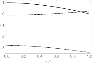
Figure 1: The functions $g(r)/c_{0}$ (thick), $H(r)/c_{0}$ (dashed), $H_{T}(r)/c_{0}$ (dot-dashed) for $k=2r_{0}$.

III.2 The boundary metric and the stress-energy tensor

Thanks to the restricted form of our perturbation (21), one can transform the metric into the Fefferman-Graham form by the coordinate transformation:

$$r(z)=\frac{1}{z\left(1-\frac{r_{0}^{5}z^{5}}{10}\right)}+O(z^{-7}).$$ (30)

Then, the boundary metric $g_{(0)\mu\nu}$ is given by

$$g_{(0)\mu\nu}dx^{\mu}dx^{\nu}=$$

$$\frac{4}{25r_{0}^{2}}\left(1+\epsilon\,c_{0}\frac{\sin(k\rho)}{\rho}\right)d\chi^{2}-\left(1-16\epsilon\,h_{2}\frac{\sin(k\rho)}{k^{2}\rho}\right)dt^{2}$$

$$+\Biggl{[}1+\frac{8\epsilon}{k^{4}\rho^{3}}\Bigl{\{}2k(8h_{2}+k^{2}h_{0})\rho\cos(k\rho)$$

$$-(k^{2}h_{0}(2-k^{2}\rho^{2})+2h_{2}(8-3k^{2}\rho^{2}))\sin(k\rho)\Bigr{\}}\Biggr{]}d\rho^{2}$$

$$+\rho^{2}F(d\theta^{2}+\sin^{2}\theta d\phi^{2})+O(\epsilon^{2}),$$ (31)

where

$$F=1-\frac{8\epsilon}{k^{4}\rho^{3}}\Bigl{[}-k(8h_{2}+k^{2}h_{0})\rho\cos(k\rho)$$

$$\quad\quad\quad-\{k^{2}h_{0}+h_{2}(8-2k^{2}\rho^{2})\}\sin(k\rho)\Bigr{]}.$$ (32)

The stress-energy tensor is obtained from the metric coefficient $g_{(5)\mu\nu}$ in the Fefferman-Graham expansion (2), as explicitly shown in Eq. (A). As expected, the trace of the stress-energy tensor is zero, up to $O(\epsilon)$, i. e. , ${{g_{(5)}}^{\mu}}_{\mu}=O(\epsilon^{2})$ since the trace anomaly is zero.

Now, let us examine the ANEC along a radial null geodesic $l^{\mu}=(0,l^{t},l^{\rho},0,0)$. Up to $O(\epsilon)$, the geodesic equations of motion give

$$l^{t}=1+\frac{16\epsilon h_{2}\sin(k\rho)}{k^{2}\rho},$$

$$l^{\rho}=1+\frac{4\epsilon}{k^{4}\rho^{3}}\Bigl{[}4h_{2}k^{2}\rho^{2}\sin(k\rho)$$

$$-(8h_{2}+h_{0}\,k^{2})\{2k\rho\cos(k\rho)-(2-k^{2}\rho^{2})\sin(k\rho)\}\Bigr{]}.$$ (33)

Then, the null-null component of the stress-energy tensor is obtained from Eq. (A)

$$\left\langle~{}T_{\mu\nu}~{}\right\rangle l^{\mu}l^{\nu}=\epsilon K\times$$

$$\quad\quad\quad\frac{2k\rho\cos(k\rho)-(2-k^{2}\rho^{2})\sin(k\rho)}{\rho^{3}}+O(\epsilon^{2}),$$ (34)

where

$$K:=\frac{4\{-2k^{2}h_{5}+(c_{0}\,k^{2}-8h_{2})r_{0}^{5}\}}{3k^{4}}.$$ (35)

As expected, the NEC is locally violated unless $K=0$. On the other hand, the ANEC (1) is satisfied, up to $O(\epsilon)$ because

$$\int^{\infty}_{-\infty}\left\langle~{}T_{\mu\nu}~{}\right\rangle l^{\mu}l^{\nu}d\lambda=O(\epsilon^{2}),$$ (36)

where $\lambda$ is the affine parameter of $l^{\mu}$.

For the boundary metric $g^{(0)}_{\mu\nu}$, the higher order corrections in $\epsilon$ can be set to zero by the following argument. Let us denote the bulk metric by ${\Phi}$ . It can be expanded by

$${\Phi}={\Phi}_{0}+\epsilon{\Phi}_{1}+\epsilon^{2}{\Phi}_{2}+\epsilon^{3}{\Phi}_{3}+\cdots.$$ (37)

The equations of motion for the variables are obtained from the vacuum Einstein equations as

$${\cal L}{\Phi}_{1}=0,$$

$${\cal L}{\Phi}_{i}={S}_{i}({\Phi}_{1},\,{\Phi}_{2},\cdots,{\Phi}_{i-1}),\quad i=2,3,\cdots,$$ (38)

where ${\cal L}$ is a linear second order differential operator, and ${S}_{i}$ is a function of the variables ${\Phi}_{j},\,\,j=1,2,\cdots,i-1$. One can formally construct the solution ${\Phi}_{i}$ as ${\Phi}_{i}=\int{G}{S}_{i}d^{6}x$ in terms of the Green function ${G}$ of the linear operator ${\cal L}$ satisfying ${\cal L}{G}=\delta(x-x^{\prime})$. The boundary conditions of ${G}$ are the regularity condition at the bubble radius and the normalization condition at infinity. So, the perturbed boundary metric $\delta g^{(0)}_{\mu\nu}$ for higher corrections in $\epsilon$ can be always set to zero.

We can check that the achronality along the null geodesic curve of $l^{\mu}$ follows from choosing the parameter $h_{0}$ in Eq. (III.1) as

$$h_{0}=-8\frac{h_{2}}{k^{2}}.$$ (39)

In this case, the boundary metric reduces to

$$g_{(0)\mu\nu}dx^{\mu}dx^{\nu}=\frac{4}{25r_{0}^{2}}\left(1+\epsilon\,c_{0}\frac{\sin(k\rho)}{\rho}\right)d\chi^{2}+$$

$$\left(1-16\epsilon\,h_{2}\frac{\sin(k\rho)}{k^{2}\rho}\right)[-dt^{2}+d\rho^{2}+\rho^{2}(d\theta^{2}+\sin^{2}\theta d\phi^{2})].$$ (40)

Note that $\chi=\mbox{const.}$ hypersurface is conformally flat. This means that any two points along the null curve with the tangent vector $l^{\mu}$ cannot be connected by a timelike curve within the $\chi=\mbox{const.}$ hypersurface. Since $\partial_{\chi}$ is a spacelike Killing vector orthonomal to $l^{\mu}$, the null geodesic curve is also the fastest causal curve among the causal curves with the tangent vector $l^{\prime\mu}=l^{\mu}+A({\partial_{t}})^{\mu}+B(\partial_{\chi})^{\mu}$ with $A$, $B$ some constants ($A$ is non-negative and can vanish only when $B=0$), thereby guaranteeing the achronality of the null geodesic curve. For $k\neq 0$, one can always enforce the condition (39). Furthermore, in Fig. 2, we show that (35) never vanishes for $c_{0}\neq 0$. This implies that the achronal ANEC can be violated after a conformal transformation, as shown below.

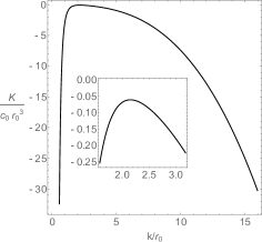
Figure 2: The function $K$ in the bubble spacetime. Notably, this never vanishes, as shown in the inset.

III.3 Conformal transformation

In the Fefferman-Graham form, the perturbed metric (21) is written by

$$ds_{6}^{2}=\frac{dz^{2}+g_{\mu\nu}(\rho,z)dx^{\mu}dx^{\nu}}{z^{2}}.$$ (41)

As done in Sec. II, one can transform the metric into a different Fefferman-Graham form

$$\hat{ds}_{6}^{2}=\frac{dZ^{2}+\hat{g}_{\mu\nu}(\xi,Z)d\hat{x}^{\mu}d\hat{x}^{\nu}}{Z^{2}},\quad\hat{x}^{\mu}=\xi,\,t,\,\theta,\,\varphi$$ (42)

with a boundary metric

$$\hat{g}_{\mu\nu}(\xi,0)d\hat{x}^{\mu}d\hat{x}^{\nu}=a^{2}(\xi)g_{\mu\nu}(\rho,0)dx^{\mu}dx^{\nu},$$ (43)

for an arbitrary scale factor $a(\xi)$.

As the coordinate transformation, we make an ansatz;

$$z(\xi,\,Z)=Z\left(\frac{1}{a(\xi)}+\alpha_{1}(\xi)Z+\alpha_{2}(\xi)Z^{2}+\cdots\right),$$

$$\rho(\xi,\,Z)=\xi+\beta_{1}(\xi)Z+\beta_{2}(\xi)Z^{2}+\beta_{3}(\xi)Z^{3}+\cdots.$$ (44)

By substituting these into Eq. (41) and keeping the metric form (42), each coefficient is determined by

$$\alpha_{2i+1}=\beta_{2i+1}=0\quad\mbox{for}\quad i\in 0,1,2,\cdots,$$

$$\alpha_{2}=-\frac{a^{\prime 2}}{4a^{5}R_{0}},\qquad\beta_{2}=\frac{a^{\prime}}{2a^{3}R_{0}},$$

$$\alpha_{4}=\frac{2a^{2}a^{\prime 2}R_{2}+a^{\prime 4}}{16a^{9}R_{0}^{2}},$$

$$\beta_{4}=-\frac{a^{\prime}}{16a^{7}R_{0}}\{2R_{0}(2a^{2}R_{2}+a^{\prime 2})+aa^{\prime}R_{0}^{\prime}\},\cdots,$$ (45)

where $R_{i}$ is the coefficient in the expansion of $g_{\rho\rho}$,

$$g_{\rho\rho}=R_{0}(\xi)+R_{2}(\xi)z^{2}+R_{4}(\xi)z^{4}+\cdots.$$ (46)

Under the coordinate transformation, the boundary metric satisfies Eq. (43) and the stress-energy tensor are transformed into

$$\hat{T}_{\mu\nu}=\frac{1}{a^{3}(\xi)}T_{\mu\nu}.$$ (47)

Since this is the conformal transformation on the boundary metric, the achronal null geodesic orbit does not change and the tangent vector is transformed by

$$\hat{l}^{\mu}=\frac{1}{a^{2}(\xi)}l^{\mu}.$$ (48)

Hence, the averaged null energy condition is transformed into

$$\int^{\infty}_{-\infty}\left\langle~{}\hat{T}_{\mu\nu}~{}\right\rangle\hat{l}^{\mu}\hat{l}^{\nu}d\hat{\lambda}=\int^{\infty}_{-\infty}\frac{1}{a^{5}}\left\langle~{}T_{\mu\nu}~{}\right\rangle l^{\mu}l^{\nu}d\lambda,$$ (49)

where we used the fact that $d\hat{\lambda}=a^{2}d\lambda$ for the affine parameter $\hat{\lambda}$ for the null geodesic in $(\partial M,\hat{g})$. This implies that for a suitable choice of the scale factor $a$, this becomes negative unless $K=0$ in Eq. (35). As an explicit simple example, choose

$$a(\xi)=(1+b^{2}e^{-k^{2}\xi^{2}})^{-1/5}$$ (50)

for real $b$ which gives

$$\int_{-\infty}^{\infty}\frac{1}{a^{5}}\left\langle~{}T_{\mu\nu}~{}\right\rangle l^{\mu}l^{\nu}d\lambda$$

$$\quad\quad=-2k^{2}b^{2}K\left(\frac{\sqrt{\pi}}{\sqrt[4]{e}}-\pi\text{Erf}\left(\frac{1}{2}\right)\right)\epsilon+O(\epsilon^{2})<0.$$ (51)

III.4 The generic condition in the bulk

Compared with the bubble solution with high symmetry in Sec. II, it is not immediate obvious whether or not the perturbed bubble solution is causally proper. However, as shown in the Gao-Wald theorem GaoWald , the condition of being causally proper is always satisfied provided that the following three conditions are satisfied in the bulk:

1. the NEC holds for the bulk null geodesics,

2. no causal pathologies are observable from the boundary, e.g. singularities or regions of causality violation,

3. the null generic condition holds for the bulk null geodesics 

The only non-trivial check is the final condition 3, as the perturbed vacuum spacetime automatically satisfies the first and the second conditions. If there existed a bulk null geodesic orbit with tangent vector $k^{a}$ that connects two points on the boundary achronal null geodesic with the tangent vector $l^{\mu}$, the orbit of $k^{a}$ would have to be sufficiently near the conformal boundary, and hence, $k^{z}$ would be small, i. e., $k^{z}=O(\epsilon)$ because we consider only perturbations of the bubble spacetime (III) which is causally proper. The Weyl tensor in the bulk behaves as $C_{cadb}k^{a}k^{b}\sim C_{a\mu b\nu}l^{\mu}l^{\nu}=O(\epsilon)$. For example,

$$C_{\chi\mu\chi\nu}l^{\mu}l^{\nu}\sim\epsilon\frac{2k\rho\cos(k\rho)-(2-k^{2}\rho^{2})\sin(k\rho)}{\rho^{3}}.$$ (52)

Then, the null geodesic would necessarily pass through a point in which the generic condition is satisfied. This is impossible by the theorem GaoWald .

IV Time delay and the weak cosmic censorship in AdS

In the previous section, we have shown within perturbative framework that the spacetime considered is causally proper from the Gao-Wald theorem GaoWald . We can also deduce from similar arguments to those in the Gao-Wald theorem the following Proposition concerning weak cosmic censorship in asymptotically AdS spacetimes.

Proposition.
Suppose $(M,\,g_{ab})$ is an asymptotically AdS spacetime, which can be conformally embedded in an unphysical spacetime $(\tilde{M},\,\tilde{g}_{ab})$ so that with a smooth function $\Omega$ in $\tilde{M}$, we have $\tilde{g}_{ab}=\Omega^{2}g_{ab}$ and $\Omega=0$ on the timelike boundary $\partial M$ in $\tilde{M}$. Suppose $(M,\,g_{ab})$ satisfies the following conditions,

• the NEC and the null generic condition,

• $\bar{M}:=M\cup\partial M$ is strongly causal, and $\partial M$ itself is globally hyperbolic.

If there is a causal curve in $\bar{M}$ from a point $p\in\partial M$ connecting to a point $q\in E^{+}(p,\,\partial M)\setminus\{p\}$ which passes through points in the bulk $M$ (i.e., which is not entirely in $\partial M$), then there must be a past-incomplete null geodesic curve in $M$ from a point of $\partial M$. That is, there is a singularity in $M$ visible from a boundary point in the future of $p$, implying a violation of weak cosmic censorship.

Proof.
Let us consider $p\in\partial M$ and $E^{+}(p,\partial M)$. Let $q$ be a point in $E^{+}(p,\partial M)\setminus\{p\}$ and $\lambda$ be a null geodesic generator of $E^{+}(p,\partial M)$ that connects $p$ and $q$. Then, by assumption, there exists a future-directed causal curve $\mu$ in $\bar{M}$ from $p$ to the future end point $q$, passing through the bulk $M$. Now suppose that $\mu$ is a null geodesic generator of $\dot{J}^{+}(p,\bar{M})$. Then, $\mu$ must be an achronal null geodesic and also be complete as it connects the two points $p,q$ at infinity ($\partial M$). However, if $\mu$ is a complete null geodesic in $M$, it would admit a pair of conjugate points due to the condition (i), and hence fail to be an achronal null geodesic, according to the proposition 4.5.12 in HawkingEllis . Thus, $\mu$ cannot be a null geodesic generator of $\dot{J}^{+}(p,\bar{M})$. By the proposition 4.5.10 in HawkingEllis , $p$ and $q$ can be joined by a timelike curve, implying in particular that the future end point $q$ of $\mu$ cannot be in $E^{+}(p,\bar{M})$. Then, since $\lambda\cap E^{+}(p,\bar{M})\setminus\{p\}\neq\emptyset$ by the condition (ii), there must be a future end point $r$ of $\lambda\cap E^{+}(p,\bar{M})$ such that $r\in J^{-}(q,\partial M)\setminus\{q\}$ and $r$ is intersected by a bulk null geodesic generator $\gamma$ of $\dot{J}^{+}(p,\bar{M})$, which entirely lies in $M$ except their end points on $\partial M$.

If $\gamma$ had a past endpoint, $\gamma$ would be a generator of $E^{+}(p,\,\bar{M})$ with the past end point $p$. But, this is a contradiction, since there would be a pair conjugate points along $\gamma$ between $p$ and $r$, and hence $\gamma$ could not be a generator of $E^{+}(p,\bar{M})$, again by the proposition 4.5.12 in HawkingEllis . Thus, $\gamma$ has no past end point. If $\gamma$ were past-complete inextendible null geodesic, there would be a pair conjugate points along $\gamma$ which also leads to contradiction. So, $\gamma$ must terminate at a singularity in the past direction. Since $\gamma$ is future directed from $p\in\partial M$, this singularity is visible from $q$, that is, nakedly singular. $\Box$

Figure 3: The solid and dashed lines represent $\lambda\in E^{+}(p,\bar{M})$ and $\gamma\in\dot{J}^{+}(p,\bar{M})$, respectively. $\gamma$ terminates at the singularity.

It may be instructive to see a concrete example. For the negative mass planar Schwarzschild-AdS spacetime, $E^{+}(p,\partial M)$ is intersected by a bulk null geodesic generator (dashed curve) of $\dot{J}^{+}(p,\bar{M})$ which terminates at singularity, as shown in Fig. 3.

V Summary and discussions

In this paper, we have explored possible interplay between the archonal ANEC, the causally proper nature of bulk and boundary spacetimes, and the weak cosmic censorship within the context of AdS/CFT duality. We have shown that the achronal ANEC can be violated in holographic theories by vacuum bubble AdS solutions. In Sec. II, we have shown a violation of the achronal ANEC in $4$-dimensional boundary CFT due to the conformal anomaly. Since the boundary spacetime is a curved spacetime, the violation does not conflict with the proof of the ANEC in the flat boundary spacetime KellyWall2014 . As shown in the Gao-Wald theorem GaoWald , our examples are “causally proper” in the sense that a “fastest null geodesic” connecting any two points on the boundary must lie entirely on the boundary. This means that there is no acausal signaling in the boundary theory, which is not physically permitted.

In Sec. III, we have shown the violation of the achronal ANEC in $5$-dimensional CFT by perturbing the $6$-dimensional vacuum bubble spacetime. In this case, since the boundary is $5$-dimensional, there is no conformal anomaly. The extent of the violation is small since the null-null component of the boundary stress-energy tensor is proportional to the amplitude of the perturbation. So, it would be interesting to investigate if the ANEC is also violated beyond the perturbation. One of the candidates is the vacuum bubble solution with a wormhole geometry in the boundary spacetime. In the thermal state, the vacuum black hole solution with a wormhole throat on the boundary has been numerically constructed IMM2018 . Even though the ANEC is not violated by the existence of the infinite thermal energy in the asymptotic flat region, negative null energy appears near the throat, caused by the negative curvature on the horizon. This leads us to speculate that the ANEC would be violated for a vacuum bubble AdS solution with a wormhole throat, as there is no asymptotic positive null energy.

In Sec. IV, we have presented a Proposition which connects the cosmic censorship in the AdS bulk to the causally proper nature of our holographic system. According to the proposition, acausal propagation of signals in the boundary theory means the occurrence of a naked singularity in the bulk. In IshibashiMaeda12 , Hawking and Penrose type singularity theorems HawkingEllis have been revisited in asymptotically AdS spacetimes, and the essential role of the strong gravity condition (i.e., the existence of a trapped set) in the bulk has been discussed. The above proposition may be viewed as a different type of singularity theorem which does not need to impose the strong gravity condition in the bulk, but which, instead, invokes the causally proper nature, as an alternative condition that involves sensible causal interactions between the bulk and the conformal boundary. This may give some new insights into possible applications of the AdS/CFT duality, in particular new connections between bulk and boundary causality.

VI Acknowledgements

We would like to thank T. Okamura for useful discussions. This work was supported in part by JSPS KAKENHI Grant Number 17K05451 (KM), 15K05092 (AI) and the European Research Council (ERC) under the European Unions Horizon 2020 research and innovation programme (grant agreement No. 758759) (EM).

Appendix A Stress energy tensor for $d=5$-dimensions

For general $g_{0},\,h_{0}$, the stress tensor is

$$g^{(5)}_{\mu\nu}dx^{\mu}dx^{\nu}=-\frac{16r_{0}^{3}}{125}\left[1+\epsilon\left(10\frac{h_{5}}{r_{0}^{5}}+c_{0}\right)\frac{\sin(k\rho)}{\rho}\right]d\chi^{2}+\frac{r_{0}^{5}}{5}\left[-1+\epsilon\left\{8h_{2}+5k^{2}\left(-8\frac{h_{5}}{r_{0}^{5}}+c_{0}\right)\right\}\frac{\sin(k\rho)}{3k^{2}\rho}\right]dt^{2}$$

$$+\frac{r_{0}^{5}}{5}\Biggl{[}1+\frac{\epsilon}{3k^{4}\rho^{3}}\Biggl{\{}8k\Bigl{(}-\frac{10k^{2}h_{5}}{r_{0}^{5}}+8h_{2}+k^{2}(5c_{0}+6h_{0})\Bigr{)}\rho\cos(k\rho)$$

$$\quad\quad\quad\quad+\Bigl{\{}-64h_{2}+k^{2}\Bigl{(}\frac{80h_{5}}{r_{0}^{5}}-8(5c_{0}+6h_{0})+3(8h_{2}+k^{2}(5c_{0}+8h_{0})\rho^{2})\Bigr{)}\Bigr{\}}\sin(k\rho)\Biggr{\}}\Biggr{]}d\rho^{2}$$

$$+\frac{r_{0}^{5}}{5}\Biggl{[}\rho^{2}+\frac{4\epsilon}{3k^{3}}\Bigl{\{}\frac{10k^{2}h_{5}}{r_{0}^{5}}-8h_{2}-k^{2}(5c_{0}+6h_{0})\Bigr{\}}\cos(k\rho)$$

$$\quad\quad\quad\quad+\frac{\epsilon}{3k^{4}}\Bigl{\{}32h_{2}+k^{2}\Bigl{(}-\frac{40h_{5}}{r_{0}^{5}}(1-k^{2}\rho^{2})+20c_{0}+24h_{0}-8h_{2}\,\rho^{2}-5c_{0}k^{2}\,\rho^{2}\Bigr{)}\Bigr{\}}\frac{\sin(k\rho)}{\rho}\Biggr{]}(d\theta^{2}+\sin^{2}\theta d\phi^{2})+O(\epsilon^{2}).$$ (53)

Appendix B Analytic solution for $r_{0}=0$

Despite being unstable to generic perturbations, it is useful to note that Eq. (III.1) can be solved analytically when $r_{0}=0$. The solutions are

$$g(r) =\frac{c_{0}}{3}\frac{e^{-k/r}(k^{2}+3kr+3r^{2})}{r^{2}}$$

$$H(r) =h_{0}+\frac{c_{0}-g(r)}{8}$$

$$=-\frac{c_{0}}{24}\left(1+\frac{e^{-k/r}(k^{2}+3kr+3r^{2})}{r^{2}}\right)$$

$$H_{T}(r) =-4h_{0}-\frac{3c_{0}+g(r)}{6}$$

$$=\frac{c_{0}}{18}\left(3-\frac{e^{-k/r}(k^{2}+3kr+3r^{2})}{r^{2}}\right)$$ (54)

The second equalities are for the choice $h_{0}=-8h_{2}/k^{2}$. For any $h_{0}$, this solution leads to

$$K=-\frac{k^{3}}{135}c_{0}.$$ (55)

At large $k$, the solution for $r_{0}\neq 0$ is approximately equal to the vacuum solution confirming that $K$ never vanishes in the perturbed bubble spacetime. The boundary metric is (to all orders in $\epsilon$)

$$g_{\mu\nu}^{(0)}dx^{\mu}dx^{\nu}=\frac{4}{25r_{0}^{2}}\left(1+\epsilon c_{0}\frac{\sin(k\rho)}{\rho}\right)d\chi^{2}+$$

$$\left(1-\epsilon\frac{c_{0}}{3}\frac{\sin(k\rho)}{\rho}\right)[-dt^{2}+d\rho^{2}+\rho^{2}(d\theta^{2}+\sin^{2}\theta d\phi^{2})].$$ (56)

and

$$l^{t}=l^{\rho}=\left[1-\epsilon\frac{c_{0}}{3}\frac{\sin(k\rho)}{\rho}\right]^{-1}.$$ (57)

For our previous choice of conformal factor $a(\xi)=(1+b^{2}\exp(-k^{2}\xi^{2}))^{-1/5}$, we find that

$$\int_{-\infty}^{\infty}\left\langle~{}T_{\mu\nu}~{}\right\rangle l^{\mu}l^{\nu}d\lambda$$

$$\quad\quad\approx-\epsilon(3.78\times 10^{-3})k^{5}b^{2}+O(\epsilon^{2})<0.$$ (58)

References

- (1) G. Klinkhammer, Phys. Rev. D43, 2542 (1991).
- (2) R. Wald and U. Yurtsever, Phys. Rev. D44, 403 (1991).
- (3) U. Yurtsever, Class. Quant. Grav. 7, L251 (1990).
- (4) L. Ford and T. A. Roman, Phys. Rev. D51, 4277 (1995).
- (5) U. Yurtsever, Phys. Rev. D51, 5797 (1995).
- (6) M. Visser, Phys. Rev. D54, 5116 (1996).
- (7) N. Graham and K. D. Olum, Phys. Rev. D76, 064001 (2007).
- (8) M. Visser, Phys. Lett. B349, 443 (1995).
- (9) D. Urban and K. D. Olum, Phys. Rev. D81, 024039 (2010).
- (10) W. R. Kelly and A. C. Wall, Phys. Rev. D90, 106003 (2014) (Erratum: Phys. Rev. D91, 069902 (2015)).
- (11) P. Arnold, P. Romatschke, and W. Schee, JHEP 10, 110 (2014).
- (12) A. Ishibashi, K. Maeda, and E. Mefford, Phys. Rev. D99, 026004 (2019).
- (13) S. d. Haro, K. Skenderis, and S. N. Solodukhin, Comm. Math. Phys. 217 595 (2001).
- (14) S. Gao and R. M. Wald, Class. Quant. Grav. 17 4999 (2000).
- (15) P. S. Apostolopoulos, G. Siopsis, and N. Tetradis, Phys. Rev. Lett. 102, 151301 (2009).
- (16) A. Chamblin and G. W. Gibbons, Phys. Rev. Lett. 84, 1090 (2000)
- (17) G. T. Horowitz and R. C. Myers, Phys. Rev. D 59, 026005 (1998)
- (18) H. Kodama and A. Ishibashi, Prog. Theor. Phys. 110 701 (2003).
- (19) M. Mars and J. M.M. Senovilla, Class. Quant. Grav. 10 1633 (1993).
- (20) S. W. Hawking and G. F. R. Ellis, “The large scale structure of spacetime”, Cambridge University Press (1973).
- (21) A. Ishibashi and K. Maeda, Phys. Rev. D86, 104012 (2012).