Abstract

Coalescent theory combined with statistical modeling allows us to estimate effective population size fluctuations from molecular sequences of individuals sampled from a population of interest. When sequences are sampled serially through time and the distribution of the sampling times depends on the effective population size, explicit statistical modeling of sampling times improves population size estimation. Previous work assumed that the genealogy relating sampled sequences is known and modeled sampling times as an inhomogeneous Poisson process with log-intensity equal to a linear function of the log-transformed effective population size. We improve this approach in two ways. First, we extend the method to allow for joint Bayesian estimation of the genealogy, effective population size trajectory, and other model parameters. Next, we improve the sampling time model by incorporating additional sources of information in the form of time-varying covariates. We validate our new modeling framework using a simulation study and apply our new methodology to analyses of population dynamics of seasonal influenza and to the recent Ebola virus outbreak in West Africa.

1 Introduction

Phylodynamic inference—the study and estimation of population dynamics from genetic sequences—relies upon data sampled in a timeframe compatible with the evolutionary dynamics under question [Drummond et al., 2003]. One important class of phylodynamic methods seeks to estimate magnitudes and changes in a measure of genetic diversity called the effective population size, often considered proportional to the census population size [Wakeley and Sargsyan, 2009] or number of infections in epidemiological contexts [Frost and Volz, 2010]. One subtle and often ignored complication of phylodynamic inference occurs when there is a probabilistic dependence between the effective population trajectory and the temporal frequency of collecting data samples, such as in case of sampling infectious disease agent genetic sequences with increasing urgency and intensity during a rising epidemic. This issue of preferential sampling was studied in depth by Karcher et al. [2016] in the limited context of a known, fixed genealogy reconstructed from the genetic data, revealing that sampling protocols that (implicitly) depend on effective population size cause model misspecification bias in models that do not account for the possibility of preferential sampling. Here, we extend the work of Karcher et al. [2016] and develop a Bayesian framework for accounting for preferential sampling during effective population size estimation directly from sequence data rather than from a fixed genealogy. We also propose a more flexible model for sequence sampling times that allows for inclusion of arbitrary time-dependent covariates and their interactions with the effective population size.

Methods for estimating effective population size from genealogical data and genetic sequence data have evolved from the earliest low dimensional parametric methods, such as constant population size [Griffiths and Tavaré, 1994b] and exponential growth models [Griffiths and Tavaré, 1994b, Drummond et al., 2002], to more flexible, nonparametric or highly parametric methods based on change-point models and Gaussian process smoothing [Drummond et al., 2005, Heled and Drummond, 2008, Minin et al., 2008, Palacios and Minin, 2013, 2012, Gill et al., 2013, 2016]. Most coalescent-based methods condition on the times of sequence sampling, rather than include these times into the model, leaving open the possibility of model misspecification if preferential sampling over time is in play. Volz and Frost [2014] and Karcher et al. [2016] introduced coalescent models that include sampling times as random variables, whose distribution is allowed to depend on the effective population size. In particular, Karcher et al. [2016] propose a method that models sampling times as an inhomogeneous Poisson process with log-intensity equal to an affine transformation of the log-transformed effective population size. In the presence of preferential sampling, this sampling-aware model demonstrates improved accuracy and precision compared to standard coalescent models due to eliminating an element of model misspecification and incorporating an additional source of information to estimate the effective population trajectory.

The main limitations of the approach of Karcher et al. [2016] are a reliance on a fixed, known genealogy and lack of flexibility in the preferential sampling time model that currently does not allow the relationship between effective population size and sampling intensity to change over time. We address the issue of fixed-tree inference by implementing a preferential sampling time model in the popular phylodynamic Markov chain Monte Carlo (MCMC) software package BEAST [Suchard et al., 2018]. This allows us to perform inference directly from genetic sequence data, appropriately accounting for genealogical uncertainty, using a wide selection of molecular sequence evolution models and well tested phylogenetic MCMC transition kernels. Additionally, we implement a tuning parameter free elliptical slice sampling transition kernel [Murray et al., 2010] for high dimensional effective population size trajectory parameters, which allows us to update these parameters efficiently.

We also address the issue of an inflexible preferential sampling time model by incorporating time-varying covariates into the model. We model the sampling times as an inhomogeneous Poisson process with log-intensity equal to a linear combination of the log-effective population size and any number of functions of time. These functions can include time varying covariates and products of covariates and the log-effective population size, referred to as interaction covariates. The addition of covariates into the sampling time model allows for incorporating additional sources of information into the relationship between effective population size and sampling intensity. One example of time-varying covariates includes an exponential growth function to account for a continuous decrease in sequencing costs that results in increased intensity of genetic data collection over time. In the context of endemic infectious disease surveillance, it is likely important to account for seasonality when modeling changes in genetic data sampling intensity, motivating inclusion of periodic functions as time varying covariates in the preferential sampling model.

We validate our methods first by simulating genealogies and sequence data and confirming that our methods successfully reconstruct the true effective population trajectories and true model parameters. We briefly simulate data in a fixed-tree context to demonstrate the fundamentals of incorporating covariates into the sampling time model and what bias is introduced by model misspecifications. We proceed to simulate genetic sequence data and demonstrate that our model successfully functions when we estimate effective population size trajectory and other parameters directly from sequence data. We also use simulations to test a combination of the two extensions of the preferential sampling model and work with covariates while sampling over genealogies during the MCMC. Finally, we use our method to analyze two real-world epidemiological datasets. We analyze a USA/Canada regional influenza dataset [Zinder et al., 2014] to determine if exponential growth of genetic sequencing or seasonal changes in sampling intensity are important to adjust for during effective population size reconstruction. We also analyze data from the recent Ebola outbreak in Western Africa to determine if preferential sampling has taken place and whether time-varying covariates or interaction covariates improve the phylodynamic inference.

2 Methods

2.1 Sequence Data and Substitution Model

Consider an alignment $\mathbf{y}=\{y_{ij}\}$, $i=1,\dots,n$, $j=1,\dots,l$, of $n$ genetic sequences across $l$ sites, collected from a well-mixed population at sampling times

$${\mathbf{s}=\{s_{i}\}_{i=1}^{n},\>\allowbreak s_{1}\geq\ldots\geq s_{n}=0.}$$

The following example shows an alignment of $n=5$ samples across $l=10$ sites, sampled at distinct times between time 7 and time 0—with time understood to be time before the latest sample:

$$\mathbf{y}_{1}=\> ACATGAGCTT,\; s_{1}=7$$

$$\mathbf{y}_{2}=\> ACTTGACCTG,\; s_{2}=4$$

$$\mathbf{y}_{3}=\> TCTTGACCTT,\; s_{3}=2$$

$$\mathbf{y}_{4}=\> AAATCTGCGT,\; s_{4}=1$$

$$\mathbf{y}_{5}=\> AGATGTGCAT,\; s_{5}=0.$$

All of the individual sequences share a common ancestry, which can be represented by a bifurcating tree called a genealogy—illustrated in Figure 1.

Figure 1: Illustration of an example heterochronous genealogy with $n=5$ lineages. Sampling times $s_{1},\ldots,s_{5}$ and coalescent times $t_{1},\ldots,t_{5}$ are marked below the genealogy, and sequence data $\mathbf{y}_{1},\ldots,\mathbf{y}_{5}$ are marked at their corresponding tips.

We assume that sequence data $\mathbf{y}$ are generated by a continuous time Markov chain (CTMC) substitution model that models the evolution of the genetic sequence along the genealogy $\mathbf{g}$. According to this model, alignment sites are independent and identically distributed, with a transition matrix $\boldsymbol{\theta}$ controlling the CTMC substitution rates between the different nucleotide bases. Some relaxation of these assumptions is possible [Shapiro et al., 2005]. Different substitution models are then defined by different parameterizations of $\boldsymbol{\theta}$ [Hein et al., 2004]. It is simple to simulate from these models, and we can efficiently compute the probability of the observed sequence data $\mathbf{y}$,

$$\text{Pr}(\mathbf{y}\mid\mathbf{g},\boldsymbol{\theta}),$$

using Felsenstein’s pruning algorithm [Felsenstein, 1973, 1981].

2.2 The Coalescent

Recall that we assume that the $n$ sampled sequences share a common ancestry, which can be represented by a bifurcating tree called a genealogy—illustrated in Figure 1. The branching events of the tree $\mathbf{g}=\{t_{i}\}_{i=1}^{n-1},\allowbreak{t_{1}>\ldots>t_{n-1}}$ (with $t$ greater the farther back in time an event occurs) are called coalescent events. The times associated with the tips of the tree $\mathbf{s}=\{s_{i}\}_{i=1}^{n}$, $s_{1}\geq\ldots\geq s_{n}$ are called sampling times or sampling events. If all of the sampling events are simultaneous, the sampling is called isochronous. Assuming that the population evolves according to the Wright-Fisher model of genetic drift and that the size of the population is not changing, Kingman [1982] derived a probability density for an isochronous genealogy, where the population size plays the role of a parameter of this density. Since the Wright-Fisher model is a simplified representation of the evolutionary process, the above parameter is called the effective population size, $N_{e}$. Later extensions to the coalescent model incorporated variable effective population size $N_{e}(t)$ [Griffiths and Tavaré, 1994b] and the ability to evaluate densities of genealogies with heterochronously sampled tips—genealogies with non-simultaneous sampling times [Felsenstein and Rodrigo, 1999].

Given sampling times $\mathbf{s}$ and effective population size trajectory $N_{e}(t)$, we would like to define the probability density for a particular genealogy $\mathbf{g}$. We use the term active lineages, $n(t)$, to refer to the difference between the number of samples taken and the number of coalescent events occurred between times $0$ and $t$. To illustrate, in Figure 1, $n(t)$ can be seen as the number of horizontal lines that a vertical line at time $t$ will cross. Suppose we partition the interval $(s_{n},t_{1})$, from the most recent sampling event to the time to most recent common ancestor (TMRCA), into intervals $I_{i,k}$ with constant numbers of active lineages. Let $\lambda_{c}(t)=\binom{n(t)}{2}/N_{e}(t)$. Then the coalescent density evaluated at genealogy $\mathbf{g}$ is

$$\Pr(\mathbf{g}\mid N_{e}(t),\mathbf{s})\propto\prod_{k=2}^{n}{\left[\lambda_{c}(t_{k-1})\exp\left(-\int_{I_{i,k}}{\lambda_{c}(t)dt}\right)\right]}.$$ (1)

2.3 Population Size Prior

Note that without further assumptions the effective population size trajectory function $N_{e}(t)$ is infinite-dimensional, so inference about $N_{e}(t)$ without some manner of constraint is intractable. A number of approaches, reviewed in the Introduction, have been suggested to address this fact. Here, we take a regular grid approach that was used before in multiple studies [Palacios and Minin, 2012, Gill et al., 2013, 2016, Karcher et al., 2016]. To review, we approximate $N_{e}(t)$ with a piecewise constant function, $N_{\boldsymbol{\gamma}}(t)=\exp[\boldsymbol{\gamma}(t)]$, where $\boldsymbol{\gamma}(t)=\sum_{i=1}^{p}{\gamma_{i}1_{\{t\in J_{i}\}}}$ and $J_{1},\ldots,J_{p}$ are consecutive time intervals of equal length. In contexts where the genealogy is known, we choose intervals that perfectly cover the interval between the TMRCA and the latest sample. However, in contexts where the genealogy is estimated from sequence data, the TMRCA is not necessarily fixed. To address this, we choose equal intervals that extend to a fixed point in time and append an additional interval that extends from that point infinitely back in time. This allows us to estimate the effective population trajectory with user-defined resolution over a window that extends back in time as far as the user chooses. The choice of the end point of the grid is up to the user, but it is advisable to choose a point that is farther back in time than an a priori estimate of the TMRCA in order to extend the high-resolution grid to cover the entire true genealogy.

The population size trajectory $N_{\boldsymbol{\gamma}}(t)$ is parameterized by a potentially high dimensional vector $\boldsymbol{\gamma}=(\gamma_{1},\ldots,\gamma_{p})$. We assume that a priori $\boldsymbol{\gamma}$ follows a first order Gaussian random walk prior with precision hyperparameter $\kappa$: $\gamma_{i}\mid\gamma_{i-1}\sim\mathcal{N}(\gamma_{i-1},1/\kappa)$ or, equivalently, that $\gamma_{i}-\gamma_{i-1}\sim\mathcal{N}(0,1/\kappa)$, for $i=2,\dots,p$. We use a Gaussian prior on the first element: $\gamma_{1}\sim\mathcal{N}(0,\sigma_{p}^{2})$. Finally, we assign a $\text{Gamma}(\alpha,\beta)$ hyperprior to $\kappa$.

2.4 Preferential Sampling Model with Covariates

Karcher et al. [2016] model times at which sequences are collected as a Poisson point process with intensity $\lambda_{s}(t)$ equal to a log-linear function of the log effective population size. Although it is realistic to assume that the larger the population, the more members of the population gets sequenced, other factors may influence the distribution of sequence sampling times. For instance, decreasing sequencing costs may result in increasing sequence sampling intensity even if the population size remains constant. We propose an extension to the sampling model that allows for the incorporation of time-varying covariates as additional sources of information. Suppose we have one or more real-valued functions, $\mathcal{F}=\{f_{2}(t),\ldots,f_{m}(t)\}$. We let

$$\log\lambda_{s}(t;\mathcal{F})=\beta_{0}+\beta_{1}\gamma(t)+\beta_{2}f_{2}(t)+\ldots+\beta_{m}f_{m}(t)+\left[\delta_{2}f_{2}(t)+\ldots+\delta_{m}f_{m}(t)\right]\gamma(t),$$ (2)

where we may set any or all of the $\beta_{2},\dots,\beta_{m}$ or $\delta_{2},\dots,\delta_{m}$ to zero if we want to avoid modeling effects of certain covariates or their interactions with the log-population size. Notice that we reserve $f_{1}(t)$ for $\gamma(t)=\log[N_{e}(t)]$, which is the covariate that is always present in our model. We also point out that even though Equation (2) is written in continuous time, in practice we assume that both the sampling intensity $\lambda_{s}(t)$ and our time varying covariates are piecewise constant, with changes occurring at the grid points specified in Subsection 2.3. We assign independent $\mathcal{N}(0,\sigma_{s}^{2})$ priors for all components of the preferential sampling model parameter vector $\boldsymbol{\beta}=(\beta_{0},\beta_{1},\dots,\beta_{m},\delta_{2},\dots,\delta_{m})$.

2.5 Posterior Approximation with MCMC

Having specified all parts of our data generating model, we are now ready to define the posterior distribution of all unknown variables of interest:

$$\begin{split}\Pr(\mathbf{g},\boldsymbol{\gamma},\kappa,\boldsymbol{\beta},\boldsymbol{\theta}\mid\mathbf{y},\mathbf{s},\mathcal{F})\propto&\Pr(\mathbf{y}\mid\mathbf{g},\boldsymbol{\theta})\Pr(\mathbf{g}\mid\boldsymbol{\gamma},\mathbf{s})\Pr(\mathbf{s}\mid\boldsymbol{\gamma},\boldsymbol{\beta},\mathcal{F})\Pr(\boldsymbol{\gamma}\mid\kappa)\\ &\times\Pr(\kappa)\Pr(\boldsymbol{\beta})\Pr(\boldsymbol{\theta}),\end{split}$$ (3)

where all probabilities and probability densities on the righthand side of equation (3) are defined in the previous subsections. Figure 2 illustrates conditional dependencies of model parameters and data in a graph form.

Figure 2: Dependency graph for the phylodynamic model parameters and data. Dependencies labeled 1 are explored in section 2.1, those labeled 2 are explored in section 2.2, those labeled 3 are explored in section 2.3, and those labeled 4 are explored in section 2.4. The dashed lines between $\boldsymbol{\gamma},\boldsymbol{\beta},\mathcal{F}$ and $\mathbf{s}$ represent preferential sampling.

When the distribution of sampling times does not depend on the effective population size trajectory (in our model, this happens when $\beta_{1}=0$ and $\delta_{2}=\cdots=\delta_{m}=0$), the posterior takes the following form:

$$\begin{split}\Pr(\mathbf{g},\boldsymbol{\gamma},\kappa,\boldsymbol{\theta},\boldsymbol{\beta}\mid\mathbf{y},\mathbf{s},\mathcal{F})&\propto\underbrace{\Pr(\mathbf{y}\mid\mathbf{g},\boldsymbol{\theta})\Pr(\mathbf{g}\mid\boldsymbol{\gamma},\mathbf{s})\Pr(\boldsymbol{\gamma}|\kappa)\Pr(\kappa)\Pr(\boldsymbol{\theta})}_{\propto\Pr(\mathbf{g},\boldsymbol{\gamma},\kappa,\boldsymbol{\theta}\mid\mathbf{y},\mathbf{s})}\\ &\times\underbrace{\Pr(\mathbf{s}\mid\boldsymbol{\beta},\mathcal{F})\Pr(\boldsymbol{\beta})}_{\propto\Pr(\boldsymbol{\beta}\mid\mathbf{s},\mathcal{F})}.\end{split}$$

The factorization above demonstrates that when $\boldsymbol{\gamma}$ is absent from the $\text{Pr}(\mathbf{s}\mid\cdot)$ term, joint and separate estimations of effective population size parameters $\boldsymbol{\gamma}$ and preferential sampling model parameters $\boldsymbol{\theta}$ will yield identical results. Moreover, in this case estimation of sampling model parameters can be dropped from the analysis entirely, since typically these parameters would be considered nuisance. If we drop preferential sampling, our model specifications reduces to the Bayesian skygrid model of Gill et al. [2013], with the corresponding posterior:

$$\Pr(\mathbf{g},\boldsymbol{\gamma},\kappa,\boldsymbol{\theta}\mid\mathbf{y},\mathbf{s})\propto\Pr(\mathbf{y}\mid\mathbf{g},\boldsymbol{\theta})\Pr(\mathbf{g}\mid\boldsymbol{\gamma},\mathbf{s})\Pr(\boldsymbol{\gamma}|\kappa)\Pr(\kappa)\Pr(\boldsymbol{\theta}).$$ (4)

We approximate posteriors (3) and (4) by devising MCMC algorithms, implemented in the software package BEAST [Suchard et al., 2018], that target these distributions. We update model parameters in blocks — 1) genealogy $\mathbf{g}$, 2) substitution parameters $\boldsymbol{\theta}$, 3) population size parameters $\boldsymbol{\gamma}$, 4) random walk prior precision $\kappa$, 5) preferential sampling model parameters $\boldsymbol{\beta}$ — keeping parameters outside of the block fixed. We update the genealogy and substitution model parameters via the default BEAST Markov kernels. We update the log effective population latent field $\boldsymbol{\gamma}$ via an elliptical slice sampler (ESS) operator [Murray et al., 2010, Lan et al., 2015], which takes advantage of the Gaussian prior distribution of the latent field to perform efficient updates. Informally, it does this by sampling a set of parameter values from the prior and iteratively moving the values closer to the current values via elliptical interpolation if the coalescent likelihood falls below a random, but small, neighborhood of the current likelihood. Because the stepwise differences of the log effective population size trajectory, $\Delta\boldsymbol{\gamma}$, are modeled as independent Gaussians with precision $\kappa$, and because we give $\kappa$ a Gamma($\alpha$, $\beta$) hyperprior, we update $\kappa$ using a Normal-Gamma Gibbs update kernel with full conditional

$$\kappa\mid\Delta\boldsymbol{\gamma}\sim\text{Gamma}\left[\alpha+\frac{p}{2},\beta+\frac{1}{2}\sum_{i=2}^{p}{\left(\gamma_{i}-\gamma_{i-1}\right)^{2}}\right],$$

where $p$ is the number of parameters in the latent field. For our sampling conditional model with posterior (4), we finish here and refer to the method as ESS/BEAST, abbreviated when appropriate as ESS. For our sampling-aware model with the posterior (3), we update components of the preferential sampling model parameter vector $\boldsymbol{\beta}$ with univariate Gaussian random walk Metropolis-Hastings kernels. We refer to the method as SampESS/BEAST, abbreviated when appropriate as SampESS.

3 Implementation

We implemented INLA-based, fixed-genealogy BNPR-PS method with simple covariates in R package phylodyn (https://github.com/mdkarcher/phylodyn). The package has also MCMC functionality that can handle inference from a fixed genealogy with simple and interaction sampling model covariates. See phylodyn vignettes for more details. MCMC for direct inference from sequence data is available in the development branch of software package BEAST (https://github.com/beast-dev/beast-mcmc). We provide examples of how to specify our preferential sampling models in BEAST xml files at https://github.com/mdkarcher/BEAST-XML.

4 Results

4.1 Simulation Study

4.1.1 Inference Assuming Fixed Genealogy

In Section 2.4, we proposed an extended sampling time model that incorporated time-varying covariates. We perform a simulation study to confirm the ability of our method to recover the true effective population trajectory and model coefficients with covariates affecting the sampling intensity. We begin here with fixed genealogies and move on to direct inference from sequence data in the next section.

We start with the inhomogeneous Poisson process sampling model with log-intensity as in Equation 2. If we restrict all $\beta$s and $\delta$s to be zero aside from $\beta_{0}$, the model collapses to homogenous Poisson process sampling (equivalently, uniformly sampling a Poisson number of points across the sampling interval). If we allow $\beta_{1}$ to be nonzero, the model becomes the sampling-aware model of Karcher et al. [2016]. If we allow additional $\beta$s, each corresponding to a fixed function of time, to be nonzero (but not $\delta$s) we say that the model includes simple or ordinary covariates.

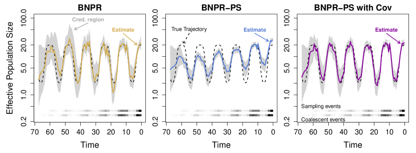
Figure 3: Effective population size reconstruction for BNPR, BNPR-PS, and BNPR-PS with simple covariates. The dotted black line represents the true effective population trajectory. The solid colored line represents the marginal posterior median effective population trajectory inferred by BNPR (yellow), BNPR-PS (blue), and BNPR-PS with simple covariates (purple), and the gray region represents the corresponding pointwise 95% credible intervals for the effective population trajectory. The log sampling intensity was $1.557+\gamma(t)-0.025t$.

For computational efficiency in this simulation study, we build upon the methods of Karcher et al. [2016], including Bayesian Nonparametric Population Reconstruction (BNPR) which uses integrated nested Laplace approximation (INLA) to efficiently approximate the marginal posterior for fixed-genealogy data, and Bayesian Nonparametric Population Reconstruction with Preferential Sampling (BNPR-PS) which does the same but includes our sampling time model (without covariates). We incorporate our extended sampling time model into BNPR-PS, but due to constraints in the INLA R package, upon which BNPR-PS relies, we can only include simple covariates.

Because our sampling time model is an inhomogeneous Poisson process, it is straightforward to simulate sampling times. We use a time-transformation method [Çinlar, 1975, pages 98–99], which, informally, treats the waiting times between events as transformations of exponential waiting times based on the intensity function following the previous event. Because the coalescent likelihood is sufficiently similar to an inhomogeneous Poisson process, we can use a similar time-transformation technique to generate the coalescent events of simulated genealogies [Slatkin and Hudson, 1991]. We implement these methods for simulating sampling times and coalescent times in R package phylodyn [Karcher et al., 2017].

In Figure 3, we illustrate BNPR, BNPR-PS, and BNPR-PS with simple covariates applied to a single simulated genealogy with sampling events distributed according to log-intensity $1.56+\gamma(t)-0.05t$, resulting in 1013 tips, where $\gamma(t)=\log[N_{e,2,6}(t)]$ and $N_{e,a,o}(t)$ is a family of functions that approximate seasonal changes in effective population size, defined as follows:

$$N_{e,a,o}(t)=\begin{cases}2+18/(1+\exp\{a[3-(t+o\mbox{ (mod 12)})]\}),&\mbox{if }t+o\mbox{ (mod 12) }\leq 6,\\ 2+18/(1+\exp\{a[3+(t+o\mbox{ (mod 12)})-12]\}),&\mbox{if }t+o\mbox{ (mod 12) }>6.\end{cases}$$ (5)

We see that BNPR (the sampling conditional model) suffers from the kind of model misspecification induced bias illustrated in [Karcher et al., 2016]. BNPR-PS with no additional covariates beyond $\gamma(t)=\log[N_{e}(t)]$, in contrast, suffers even more strongly from a misspecified sampling model. Table 1 shows that the model fails to correctly infer the coefficient of $\gamma(t)$. This illustrates the care one must take in choosing parameterizations of the sampling model. BNPR-PS with simple covariates, $\gamma(t)$ and $-t$, the correctly-specified model, produces a reconstruction of the effective population trajectory that is very close to the true trajectory used to simulate the data. Table 1 shows that the true values of the sampling model coefficients are within 95% Bayesian credible intervals produced by our inference method with the correctly specified model.

Model	Coef	Q0.025	Median	Q0.975	Truth
$\{\gamma(t)\}$	$\gamma(t)$	1.67	1.99	2.34	1.0
$\{\gamma(t),-t\}$	$\gamma(t)$	0.86	1.01	1.16	1.0
	$-t$	0.040	0.047	0.053	0.050

Table 1: Summary of simulated fixed-tree data inference. Posterior distribution quantile summaries for BNPR-PS with no covariates (model: $\{\gamma(t)\}$) and BNPR-PS with an ordinary covariate (model: $\{\gamma(t),-t\}$).

4.1.2 Direct Inference from Sequence Data

We simulate several genealogies and DNA sequences from different sampling scenarios in order to evaluate how well our population reconstruction and parameter inference performs. Given a sampling model and, optionally, an effective population size trajectory, we generate sampling times within a sampling window. We generate sampling and coalescent times for a genealogy using the same time-transformation methods as for our fixed-tree simulations. We simulate the topology of the genealogy by proceeding backward in time, adding an active lineage at each sampling time and joining a pair of active lineages uniformly at random at each coalescent event. We provide an implementation of this tree-topology simulation method in phylodyn. We generate simulated sequence alignments using the software SeqGen [Rambaut and Grassly, 1997], using the Jukes-Cantor 1969 (JC69) [Jukes et al., 1969] substitution model. We set the substitution rate to produce an expected 0.9 mutations per site, in order to produce a sequence alignment with many sites having one mutation, and some sites having zero or multiple mutations. For all of our simulations, we use the same seasonal effective population trajectory, $N_{e,2,6}(t)$, as for our fixed-tree simulations.

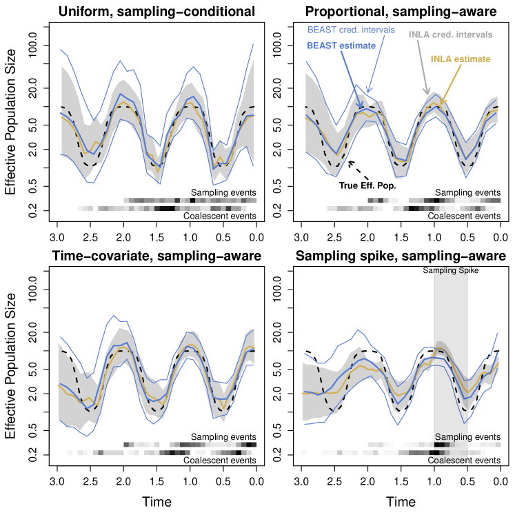
Figure 4: Effective population size reconstructions for four sequence data simulations, all based on the same seasonal effective population size trajectory. Upper left: Uniform sampling times, sampling-conditional posterior. Upper right: Sampling frequency proportional to effective population size, sampling-aware posterior. Lower left: Sampling frequency proportional to effective population times a time-covariate ($\exp(t)$), sampling- and covariate-aware posterior. Lower right: Sampling frequency proportional to effective population size with a sampling spike, sampling- and covariate-aware posterior.

First, we simulate a genealogy with 200 tips and sequence data with 1500 sites and uniform sampling times and apply both of our sampling-conditional methods. We apply the INLA-based fixed-tree BNPR from [Karcher et al., 2016] to the true genealogy, and we apply the MCMC-based tree-sampling ESS/BEAST (specified above) to the sequence data. In Figure 4 (upper left), we compare the truth with the resulting pointwise posterior medians and credible intervals. The two methods’ results are mutually consistent, with additional uncertainty in the tree-sampling method (visible in the wider credible intervals) due to having to estimate the genealogy jointly with other model parameters. We see similar results comparing BNPR-PS with SampESS/BEAST in Figure 4 (upper right), where we sample sequences (1500 sites) with sampling times generated from an inhomogeneous Poisson process with intensity proportional to effective population size (log-intensity $2.9+\gamma(t)$) resulting in 170 samples and infer using a sampling model with log-intensity $\beta_{0}+\beta_{1}\gamma(t)$. We also see similar results in Figure 4 (lower left), where we add time as an additional covariate and sample sequences (1500 sites) with log-intensity $3.35+\gamma(t)-0.5t$, resulting in 199 samples, and perform inference using a sampling model with log-intensity $\beta_{0}+\beta_{1}\gamma(t)+\beta_{2}\cdot(-t)$. Table 2 shows that SampESS does a reasonable job at reconstructing the true model coefficients, though the credible interval for $-t$ includes 0.

We also simulate a genealogy and sequence data (1500 sites) with log-intensity $1.89+\gamma(t)+\gamma(t)\cdot 1_{t\in[0.5,1]}$, resulting in 210 samples. This produces an interval we refer to as a sampling spike which requires the use of an interaction covariate. Because of design limitations of the R implementation of INLA, we are limited in how we may implement interaction covariates in BNPR-PS. Therefore, in Figure 4 (lower right) we plot SampESS/BEAST with the correct interaction covariate (and a corresponding ordinary covariate) against BNPR-PS with no covariates. We see SampESS (with covariates) perform better than BNPR-PS (without covariates) at reconstructing the correct trajectory. We also see that our method, using the full covariate model, with log-intensity $\beta_{0}+\beta_{1}\gamma(t)+\beta_{2}\cdot 1_{t\in[0.5,1]}+\delta_{2}\cdot\gamma(t)\cdot 1_{t\in[0.5,1]}$, produces a 95% Bayesian credible interval for the coefficient of the ordinary covariate that contains the true value ($\beta_{2}=0$), while the true value of the interaction covariate coefficient ($\delta_{2}=1$) is correctly inside the 95% Bayesian credible interval produced by SampESS/BEAST.

Model	Coef	Q0.025	Median	Q0.975	Truth
$\{\gamma(t)\}$	$\gamma(t)$	0.98	1.42	2.16	1.0
$\{\gamma(t),-t\}$	$\gamma(t)$	0.75	1.06	1.55	1.0
	$-t$	-0.06	0.44	0.94	0.5
$\{\gamma(t),1_{t\in[0.5,1]},1_{t\in[0.5,1]}\cdot\gamma(t)\}$	$\gamma(t)$	0.72	1.26	2.14	1.0
	$1_{t\in[0.5,1]}$	-9.01	-1.50	1.64	0.0
	$1_{t\in[0.5,1]}\cdot\gamma(t)$	0.13	1.75	5.75	1.0

Table 2: Summary of simulated sequence data inference Posterior distribution quantile summaries for SampESS with no covariates (model: $\{\gamma(t)\}$), SampESS with an ordinary covariate (model: $\{\gamma(t),-t\}$), and SampESS with both an ordinary and interaction covariate (model: $\{\gamma(t),1_{t\in[0.5,1]},1_{t\in[0.5,1]}\cdot\gamma(t)\}$).

4.2 Seasonal Influenza Example

We reanalyze the H3N2 regional influenza data for the USA/Canada region as analyzed with fixed-tree methods in [Karcher et al., 2016]. The data contain 520 sequences aligned to form a multiple sequence alignment with 1698 sites of the hemagglutinin gene. This dataset is a subset of the dataset of influenza sequences from around the world analyzed in [Zinder et al., 2014]. We use ESS/BEAST with our tree-sampling MCMC targeting posterior (4) to analyze these data and mark the pointwise posterior median and 95% credible region in black, summarized in Figure 5 (upper row). We observe a seasonal pattern consistent with flu seasons observed in the temperate northern hemisphere [Zinder et al., 2014]. Our results are also consistent with previous fixed-tree method results but with larger credible interval widths due to correctly accounting for genealogical uncertainty in our analysis.

We apply our sampling-aware model SampESS/BEAST to the USA/Canada influenza data, following the posterior from Equation (3). We used several different log-sampling-intensity models. The simplest one has log-intensity $\beta_{0}+\beta_{1}\gamma(t)$ (abbreviated $\{\gamma(t)\}$) and is summarized in Figure 5 (upper left). We include a time term in one model, with log-intensity ${\beta_{0}+\beta_{1}\gamma(t)+\beta_{2}\cdot(-t)}$ (abbreviated $\{\gamma(t),-t\}$) summarized in Figure 5 (upper center). We use seasonal indicator functions in the final model, defined as,

$$I_{\text{winter}}(t) =I_{(t\bmod 1.0)\in[0,0.25)},$$

$$I_{\text{autumn}}(t) =I_{(t\bmod 1.0)\in[0.25,0.5)},$$

$$I_{\text{summer}}(t) =I_{(t\bmod 1.0)\in[0.5,075)},$$

with $t$ measured in decimal calendar years (going forward in time). This results in the log-intensity $\beta_{0}+\beta_{1}\gamma(t)+\beta_{2}I_{\text{winter}}(t)+\beta_{3}I_{\text{autumn}}(t)+\beta_{4}I_{\text{summer}}(t)$ (abbreviated $\{\gamma(t),I_{\text{winter}},\allowbreak I_{\text{autumn}},\allowbreak I_{\text{summer}}\}$), summarized in Figure 5 (upper right).

We summarize the sampling model coefficient results for each model in Table 3. The $\{\gamma(t)\}$ model corresponds to the preferential sampling model of Karcher et al. [2016], but has noticeably different estimates. We attribute this to the differences between the fixed-tree (with a tree inferred using a constant effective population size BEAST model), INLA-based approach of Karcher et al. [2016], and the tree-sampling MCMC-based approach of this paper. We also note that the $\{\gamma(t),-t\}$ model does not perform better (or even noticeably differently) than the $\{\gamma(t)\}$ model. The coefficient summary for $\{\gamma(t),-t\}$ bears this out, because the 95% Bayesian credible interval for the coefficient for $-t$ contains 0. This is expected as each year has approximately the same number of sequences, so there should be no exponential growth of sampling intensity. We do observe differences in the $\{\gamma(t),I_{\text{winter}}$, $I_{\text{autumn}}$, $I_{\text{summer}}\}$ model. The coefficient of $\gamma(t)$ is close to 1.0, which is the easiest value to interpret under preferential sampling, suggesting a baseline sampling rate proportional to effective population size. The coefficients for the indicators suggest increased sampling in the flu season intervals, as compared to the summer intervals and especially the spring intervals—with spring treated as a baseline rate without an indicator for the sake of identifiability. We also fit a model with seasonal indicator covariates and their interactions with the log-effective population size, but do not find any support for including the interaction covariates into the preferential sampling model (see Appendix A.1).

Model	Coef	Q0.025	Median	Q0.975
$\{\gamma(t)\}$	$\gamma(t)$	1.11	1.45	2.01
$\{\gamma(t),-t\}$	$\gamma(t)$	1.21	1.52	2.00
	$-t$	-0.10	-0.02	0.07
$\{\gamma(t),I_{\text{winter}},I_{\text{autumn}},I_{\text{summer}}\}$	$\gamma(t)$	0.72	0.92	1.21
	$I_{\text{winter}}$	1.91	2.79	3.83
	$I_{\text{autumn}}$	1.88	2.85	3.85
	$I_{\text{summer}}$	0.44	1.52	2.58

Table 3: Summary of USA/Canada influenza data inference. Posterior distribution quantile summaries for SampESS with no covariates (model: $\{\gamma(t)\}$), SampESS with an ordinary covariate (model: $\{\gamma(t),-t\}$), and SampESS with seasonal indicator covariates (model: $\{\gamma(t),I_{\text{winter}},I_{\text{autumn}},I_{\text{summer}}\}$).

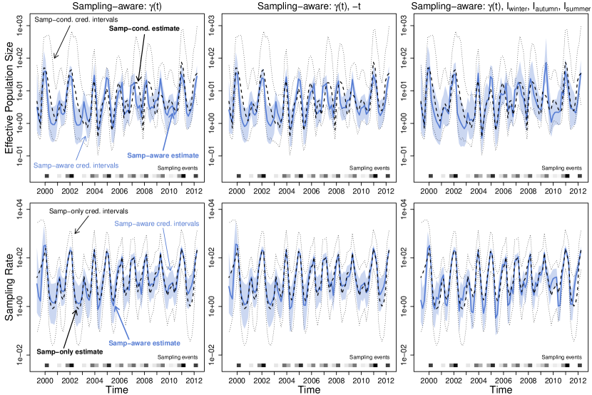
Figure 5: Effective population size and sampling rate reconstructions for the USA and Canada influenza dataset. Upper row: Dashed lines and dotted black lines are the pointwise posterior effective population size estimates and credible intervals of the sampling-conditional model. The blue lines and the light blue regions are the pointwise posterior effective population size estimates and credible intervals of that column’s sampling-aware model. Lower row: Dashed lines and dotted black lines are the pointwise posterior sampling rate estimates and credible intervals of a nonparametric sampling-time-only model. The blue lines and the light blue regions are the pointwise posterior sampling rate estimates and credible intervals of that column’s sampling-aware model.

We observe the seasonality of our estimates of the effective population size trajectory. In Figure 6, we superimpose the twelve years of estimates per model, and plot the posterior median annual estimate. We note that the sampling aware models all show increased seasonality compared to the sampling conditional model. We also note that the 2008-2009 flu season stands out on the seasonality plot for having a peak in the summer months of 2009, particularly in the preferential sampling models. This behavior is most likely due to a misspecification of our model for sampling intensity. This misspecification is expected given the first documented emergence of the H1N1 strain in the United States in April of 2009 and the resulting, unaccounted in our model, increased surveillance of all influenza strains in summer 2009 [CDC, 2010]. Higher than usual sampling intensity in summer 2009 makes our preferential sampling models conclude that the effective population size during this time period must be also elevated. Also, note that the estimated effective population size of H3N2 strain during 2009/2010 flu season is markedly lower than during most of other seasons. This is in line with the H1N1 strain successfully competing with the H3N2 strain, resulting in the lower prevalence of the latter.

To check adequacy of the preferential sampling models, we compare the posterior distributions of sampling intensities obtained via our BEAST implementation of BNPR-PS with a nonparametric INLA-based estimate of the sampling rate (using a method similar to BNPR-PS without the coalescent likelihood or covariates). Figure 5 (lower row) shows the comparison. The methods produce very similar estimates, with the BEAST/MCMC methods having thinner credible intervals due to incorporating additional information from the coalescent likelihood. We also performed posterior predictive checking, described in Appendix B.1, but found that this method lacked power to discriminate among preferential sampling models (see Appendix B.2.2).

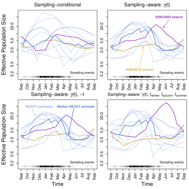
Figure 6: Effective population size seasonal overlay for the USA and Canada influenza dataset. The light blue lines are the pointwise posterior estimates for each year, and the dark blue line is the median annual estimate. Upper left: Sampling-conditional posterior. Upper right: Sampling-aware posterior with only log-effective population size $\gamma(t)$ informing the sampling time model. Lower left: Sampling- and covariate-aware posterior, with $\gamma(t)$ and $-t$. Lower right: Sampling- and covariate-aware posterior, with $\gamma(t)$ and seasonal indicators $I_{\text{winter}},I_{\text{autumn}},I_{\text{summer}}$.

4.3 Ebola Outbreak

Next, we analyze a subset of the Ebola virus sequences arising from the recent Western Africa Ebola outbreak (as collated in [Dudas et al., 2017]). The data consist of 1610 aligned whole genomes, collected from mid-2014 to mid-2015. The resulting alignment has 18,992 sites. The dataset represents over 5% of known cases of Ebola detected during that outbreak, providing an unprecedented insight into the epidemiological dynamics of an Ebola outbreak. We consider two subsets of the data, corresponding to the samples from Sierra Leone and Liberia. For Sierra Leone, we subsampled 200 sequences, chosen uniformly at random out of 1010 samples for computational tractability. For Liberia, we use the entire collection of 205 sequences obtained from infected individuals in this country.

We begin by applying ESS/BEAST method with no preferential sampling to the Sierra Leone dataset. We use MCMC to target our tree-sampling posterior from Equation (4) and depict the pointwise posterior median effective population curve, $N_{e}(t)$, with a black dashed line and its corresponding 95% credible region boundaries with black doted lines, shown in all panels of the first row of Figure 7. The resulting effective population size trajectory visually resembles a typical epidemic trajectory of prevalence or incidence that peaks in Autumn of 2014. Next, we apply our sampling-aware model SampESS/BEAST to the Ebola data, targeting with MCMC the posterior from Equation (3). We use several different log-sampling-intensity models. The simplest model, abbreviated as $\{\gamma(t)\}$, has log-sampling-intensity $\beta_{0}+\beta_{1}\gamma(t)$. We include a $t$ term in our next sampling model, abbreviated as $\{\gamma(t),-t\}$, with log-intensity ${\beta_{0}+\beta_{1}\gamma(t)+\beta_{2}\cdot(-t)}$. This model postulates that even if the effective population size remains constant, the sampling intensity is growing or declining exponentially. We make $-t$ an interaction covariate as well in the next model, abbreviated $\{\gamma(t),-t,-t\cdot\gamma(t)\}$, resulting in the log-sampling-intensity $\beta_{0}+\beta_{1}\gamma(t)+\beta_{2}\cdot(-t)+\delta_{2}\gamma(t)\cdot(-t)$. For the final model, we include $-t$ and $-t^{2}$ as ordinary covariates, abbreviated $\{\gamma(t),-t,-t^{2}\}$, with log-sampling-intensity ${\beta_{0}+\beta_{1}\gamma(t)+\beta_{2}\cdot(-t)}+\beta_{3}\cdot(-t^{2})$. The resulting posterior distribution summaries of the effective population size trajectory are shown in blue in the upper row of Figure 7.

Having concluded that posterior predictive checks are underpowered in our setting (see Appendix B.2.3), we judge preferential sampling model fit using lessons learned during simulation studies conducted by Karcher et al. [2016]. One important observation made by Karcher et al. [2016] is that ignoring preferential sampling produces little bias when estimating $N_{e}(t)$ when population size is increasing. Even during the $N_{e}(t)$ declines the bias is relatively small. Therefore, if the sampling model is not misspecified, we expect conditional and sampling aware models to differ mostly in the width of their credible intervals, and not in posterior medians of $N_{e}(t)$. According to this metric, the $\{\gamma(t),-t,-t\cdot\gamma(t)\}$ and $\{\gamma(t),-t,-t^{2}\}$ models show reasonable agreement with the conditional conditional model when reconstructing $N_{e}(t)$ (see first row of Figure 7), with the $\{\gamma(t),-t,-t\cdot\gamma(t)\}$ model performing the best. Another measure of goodness of fit is agreement of nonparametric estimate of sampling intensity and the one produced by preferential sampling models. By this metric, the quadratic model $\{\gamma(t),-t,-t^{2}\}$ outperforms the interaction model $\{\gamma(t),-t,-t\cdot\gamma(t)\}$. The main difference between the interaction and quadratic models is that the interaction model suggests that the strength of preferential sampling (power of $N_{e}(t)$) was linearly increasing over time, while the quadratic model points to a quadratically time varying multiplicative factor in front of $N_{e}(t)$. Parameter estimates of all models fit to the Sierra Leone data are summarized in Table 4.

As another way to compare adequacy of preferential sampling models, we overlay our reconstructed effective population size trajectories and Ebola weekly incidence time series. We use a sum of confirmed and probable case counts from the supplementary data of Dudas et al. [2017]. Assuming a susceptible-infectious-removed (SIR) model, an approximate structured coalescent model, and taking into account the fact that the number of susceptible individuals never decreased appreciably during the Ebola outbreak, we can interpret effective population size as a quantity proportional to Ebola incidence [Volz et al., 2009, Frost and Volz, 2010]. Figure C-1 shows aligned incidence time series and posterior summaries of effective population size for all considered coalescent models. All models produce reasonable agreement between incidence and effective population size during the increase of incidence. However, the end of the outbreak is captured better by preferential sampling models, with the quadratic model $\{\gamma(t),-t,-t^{2}\}$ outperforming the other preferential sampling models.

Model	Coef	Q0.025	Median	Q0.975
$\{\gamma(t)\}$	$\gamma(t)$	0.28	0.46	0.71
$\{\gamma(t),-t\}$	$\gamma(t)$	0.30	0.49	0.83
	$-t$	-0.58	0.27	1.46
$\{\gamma(t),-t,-t\cdot\gamma(t)\}$	$\gamma(t)$	1.01	1.76	3.32
	$-t$	-0.88	0.18	1.02
	$-t\cdot\gamma(t)$	0.89	1.65	3.11
$\{\gamma(t),-t,-t^{2}\}$	$\gamma(t)$	0.47	1.00	1.80
	$-t$	2.02	9.05	20.63
	$-t^{2}$	-13.08	-5.58	-1.09

Table 4: Summary of Sierra Leone Ebola sequence data inference. Posterior distribution quantile summaries for SampESS with no covariates (model: $\{\gamma(t)\}$), SampESS with an ordinary covariate (model: $\{\gamma(t),-t\}$), SampESS with both an ordinary and interaction covariate (model: $\{\gamma(t),-t,-t\cdot\gamma(t)\}$), and SampESS with linear and quadratic ordinary covariates (model: $\{\gamma(t),-t,-t^{2}\}$).

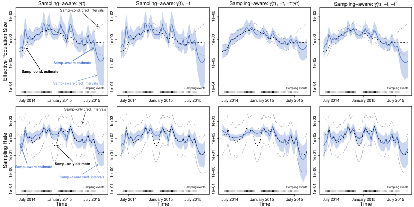
Figure 7: Effective population size and sampling rate reconstructions for the Sierra Leone Ebola dataset. Upper row: Dashed lines and dotted black lines are the pointwise posterior effective population size estimates and credible intervals of the sampling-conditional model. The blue lines and the light blue regions are the pointwise posterior effective population size estimates and credible intervals of that column’s sampling-aware model. Lower row: Dashed lines and dotted black lines are the pointwise posterior sampling rate estimates and credible intervals of a nonparametric sampling-time-only model. The blue lines and the light blue regions are the pointwise posterior sampling rate estimates and credible intervals of that column’s sampling-aware model.

Model	Coef	Q0.025	Median	Q0.975
$\{\gamma(t)\}$	$\gamma(t)$	0.53	0.78	1.20
$\{\gamma(t),-t\}$	$\gamma(t)$	0.53	0.81	1.23
	$-t$	-3.39	-0.74	1.84
$\{\gamma(t),-t,-t\cdot\gamma(t)\}$	$\gamma(t)$	-0.07	0.40	1.51
	$-t$	-3.26	-0.31	2.67
	$-t\cdot\gamma(t)$	-2.98	-1.21	1.20

Table 5: Summary of Liberia Ebola sequence data inference. Posterior distribution quantile summaries for SampESS with no covariates (model: $\{\gamma(t)\}$), SampESS with an ordinary covariate (model: $\{\gamma(t),-t\}$), and SampESS with both an ordinary and interaction covariate (model: $\{\gamma(t),-t,-t\cdot\gamma(t)\}$).

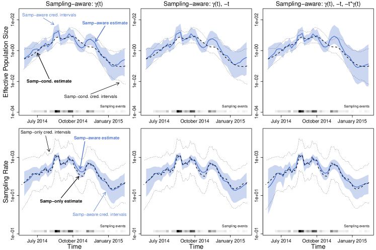
Figure 8: Effective population size and sampling rate reconstructions for the Liberia Ebola dataset. Upper row: Dashed lines and dotted black lines are the pointwise posterior effective population size estimates and credible intervals of the sampling-conditional model. The blue lines and the light blue regions are the pointwise posterior effective population size estimates and credible intervals of that column’s sampling-aware model. Lower row: Dashed lines and dotted black lines are the pointwise posterior sampling rate estimates and credible intervals of a nonparametric sampling-time-only model. The blue lines and the light blue regions are the pointwise posterior sampling rate estimates and credible intervals of that column’s sampling-aware model.

We apply the same models to the Liberia Ebola dataset, summarized across the upper row of Figure 8 and in Table 5. We note that the $\{\gamma(t)\}$ and $\{\gamma(t),-t\}$ models perform very similarly, but the $\{\gamma(t),-t\}$ model has slightly wider pointwise credible intervals in places. This is consistent with the coefficients, as the credible interval for the $-t$ term contains 0. The $\{\gamma(t),-t,-t\cdot\gamma(t)\}$ model has even wider pointwise credible intervals, and the credible intervals for the coefficients all contain 0. This suggests that in Liberia, of the three sampling-aware models, the sampling model most consistent with the data is simple preferential sampling. We also note that in the $\{\gamma(t)\}$ model, the median estimate for the coefficient for $\gamma(t)$ is close to 1.0, suggesting direct proportional sampling.

As in the previous section, we compare the sampling rates we derive from our BEAST runs to a nonparametric INLA-based estimate of the sampling rate. Figures 7 (lower row) and 8 (lower row) show the comparisons. The two methods produce very similar estimates, and again the sampling-aware methods have thinner credible intervals due to incorporating additional information from the coalescent likelihood.

All coalescent models produce reasonable agreement between estimated effective population size trajectories and Ebola incidence time series in Libera (see Appendix Fig C-2). The model without preferential sampling looks the best in this comparison, mostly because the incidence curve does not support multiple “ups” and “downs” in effective population size trajectories estimated under the preferential sampling models.

5 Discussion

Currently, few phylodynamic methods incorporate sampling time models in order to address model misspecification and take advantage of the additional information contained in sampling times in preferential sampling contexts. Even fewer methods implement sampling time models by appropriately integrating over genealogies relating the sampled genetic sequences and performing inference directly from these sequence data. We extend previous sampling time models to incorporate time-varying covariates in order to allow the sampling model to be more flexible under different scientific circumstances. We implement this sampling time model into the MCMC software BEAST, and also implement an elliptical slice sampler into BEAST for efficient MCMC draws of grid-based effective population size parameterizations.

However, the additional flexibility of the sampling time model comes with additional uncertainty around which set of covariates is the best one for a given scientific context. Unfortunately, posterior predictive checks [Gelman et al., 1996] — taking a model with a posterior sample of parameters estimated from data, using the same model and estimated parameters to simulate new data, and comparing the observed data and the simulated data — lacked sufficient power to discriminate between models in all of our applications. Including a residual term to absorb sampling times model misspecification can be a fruitful avenue of future research. However, care will need to be taken to preserve parameter identifiability.

Another approach to extending and increasing the flexibility of the sampling model is to decouple the fixed temporal relationship between effective population size and sampling intensity. Introducing an estimated lag parameter to the sampling time model would allow for cause-and-effect phenomena and delays to be accounted for within the model. Incorporating an estimated lag parameter would also allow for an additional avenue of model verification. Under most imaginable circumstances, if there is a relationship between the effective population size and sampling frequency, changes to the population size would effect sampling frequency with zero or positive delay. Estimating a credibly negative lag would be a possible indicator that some element of the model or data is worth re-examining.

In terms of flexibility, the ideal sampling time model would be a separate Gaussian latent field distinct from the (log) effective population size. However, methods for primarily phylodynamic inference with this feature would suffer from severe identifiability problems. One approach that would retain most of the flexibility of the separate Gaussian field while also retaining the identifiability of the original model would be to model the (log) effective population size and sampling intensities as correlated Gaussian processes. Estimating the correlation parameter between the two processes would allow for estimation of the preferential sampling strength.

Appendix A Appendix: Additional Sequence Data Results

A.1 Seasonal Influenza

We consider one additional model for the USA/Canada influenza data with log-intensity,

$$\beta_{0}+\beta_{1}\gamma(t) +\beta_{2}I_{\text{winter}}(t)+\beta_{3}I_{\text{autumn}}(t)+\beta_{4}I_{\text{summer}}(t)$$

$$+\delta_{2}I_{\text{winter}}(t)\cdot\gamma(t)+\delta_{3}I_{\text{autumn}}(t)\cdot\gamma(t)+\delta_{4}I_{\text{summer}}(t)\cdot\gamma(t),$$

abbreviated $\{\gamma(t)$, $I_{\text{winter}}$, $I_{\text{autumn}}$, $I_{\text{summer}}$, $I_{\text{winter}}\cdot\gamma(t)$, $I_{\text{autumn}}\cdot\gamma(t)$, $I_{\text{summer}}\cdot\gamma(t)\}$, or more succinctly as $\{\gamma(t)$, $I_{\text{winter}}$, $I_{\text{autumn}}$, $I_{\text{summer}}$, $\text{interactions}\}$. The results are summarized in Figure A-1 and Table A-1. We see that only the coefficients for $\gamma(t)$, $I_{\text{winter}}$, and $I_{\text{autumn}}$ have credible intervals that do not contain zero, suggesting that additional terms are not necessary.

Model	Coef	Q0.025	Median	Q0.975
$\{\gamma(t),I_{\text{winter}},I_{\text{autumn}},I_{\text{summer}},\text{interactions}\}$	$\gamma(t)$	0.64	1.20	1.97
	$I_{\text{winter}}$	1.83	3.48	5.58
	$I_{\text{autumn}}$	1.31	3.16	5.28
	$I_{\text{summer}}$	-0.15	2.08	4.52
	$I_{\text{winter}}\cdot\gamma(t)$	-1.08	-0.29	0.34
	$I_{\text{autumn}}\cdot\gamma(t)$	-1.00	-0.14	0.53
	$I_{\text{summer}}\cdot\gamma(t)$	-1.24	-0.24	0.92

Table A-1: Summary of USA/Canada influenza data inference. Posterior distribution quantile summaries for SampESS with seasonal indicator and interaction covariates (model: $\{\gamma(t),I_{\text{winter}},I_{\text{autumn}},I_{\text{summer}}$,$\text{interactions}\}$).

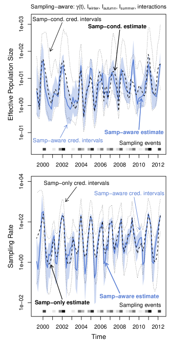
Figure A-1: Effective population size and sampling rate reconstructions for the USA and Canada influenza dataset. Upper row: Dashed lines and dotted black lines are the pointwise posterior effective population size estimates and credible intervals of the sampling-conditional model. The blue line and the light blue region are the pointwise posterior effective population size estimates and credible intervals of that column’s sampling-aware model. Lower row: Dashed lines and dotted black lines are the pointwise posterior sampling rate estimates and credible intervals of a nonparametric sampling-time-only model. The blue line and the light blue region are the pointwise posterior sampling rate estimates and credible intervals of that column’s sampling-aware model.

A.2 Ebola Outbreak

We consider three additional models for our subsample of 200 sequences from the Sierra Leone Ebola outbreak data with log-intensities,

$$\beta_{0}+\beta_{1}\gamma(t) +\beta_{2}\cdot(-t)+\beta_{3}\cdot(-t^{2})$$

$$+\delta_{2}\gamma(t)\cdot(-t)+\delta_{3}\gamma(t)\cdot(-t^{2}),\;\text{and}$$

$$\beta_{0}+\beta_{1}\gamma(t) +\delta_{2}\gamma(t)\cdot(-t)+\delta_{3}\gamma(t)\cdot(-t^{2}),$$

abbreviated as $\{\gamma(t),-t,-t^{2}$, $-t\cdot\gamma(t)$, $-t^{2}\cdot\gamma(t)\}$, and $\{\gamma(t)$, $-t\cdot\gamma(t)$, $-t^{2}\cdot\gamma(t)\}$, respectively. The results are summarized in Figure A-2 and Table A-2. We see that the coefficients for $\gamma(t)$, $-t$, and $-t^{2}$ tend to have credible intervals that do not contain zero (except for the interaction-only model $\{\gamma(t)$, $-t\cdot\gamma(t)$, $-t^{2}\cdot\gamma(t)\}$), but the other terms do not, suggesting that the additional terms are not necessary.

Model	Coef	Q0.025	Median	Q0.975
$\{\gamma(t),-t,-t^{2},-t\cdot\gamma(t),-t^{2}\cdot\gamma(t)\}$	$\gamma(t)$	0.71	2.20	4.69
	$-t$	1.21	9.75	20.29
	$-t^{2}$	-12.67	-6.00	-0.79
	$-t\cdot\gamma(t)$	-2.72	0.95	6.49
	$-t^{2}\cdot\gamma(t)$	-2.64	0.72	3.26
$\{\gamma(t),-t\cdot\gamma(t),-t^{2}\cdot\gamma(t)\}$	$\gamma(t)$	-3.00	-1.39	2.08
	$-t\cdot\gamma(t)$	-11.30	-6.59	2.00
	$-t^{2}\cdot\gamma(t)$	-0.16	4.90	8.16

Table A-2: Summary of Sierra Leone Ebola sequence data inference. Posterior distribution quantile summaries for SampESS with models: $\{\gamma(t),-t,-t^{2}$, $-t\cdot\gamma(t),-t^{2}\cdot\gamma(t)\}$, and $\{\gamma(t),-t\cdot\gamma(t),-t^{2}\cdot\gamma(t)\}$.

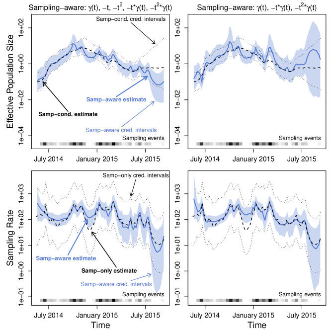
Figure A-2: Effective population size and sampling rate reconstructions for the Sierra Leone Ebola dataset. Upper row: Dashed lines and dotted black lines are the pointwise posterior effective population size estimates and credible intervals of the sampling-conditional model. The blue line and the light blue region are the pointwise posterior effective population size estimates and credible intervals of that column’s sampling-aware model. Lower row: Dashed lines and dotted black lines are the pointwise posterior sampling rate estimates and credible intervals of a nonparametric sampling-time-only model. The blue line and the light blue region are the pointwise posterior sampling rate estimates and credible intervals of that column’s sampling-aware model.

Appendix B Appendix: Model Checks and Model Selection

B.1 Methods

B.1.1 Transformed Exponentials

Suppose random variable $X\sim\text{Exp}(1)$, and thus its PDF is $f_{X}(x)=\exp(-x)$. Define ${g_{\lambda}(u)=\int_{0}^{u}{\lambda(t)dt}}$ for nonnegative $\lambda(\cdot)$ integrable on $[0,\infty)$. Then $g_{\lambda}(u)$ is monotonic nondecreasing, so $g_{\lambda}^{-1}(\cdot)$ is well-defined almost everywhere. If we let $U=g_{\lambda}^{-1}(X)$, then the PDF of $U$ is $f_{U}(u)=\lambda(u)\exp(-\int_{0}^{u}{\lambda(t)dt})$.

We then have two useful results. If we wish to sample $U$, we may do so by sampling an $\text{Exp}(1)$ random variable $X$, then apply the transformations $U=g_{\lambda}^{-1}(X)$, which will result in the desired distribution. There generally is not an explicit, closed-form solution for $g^{-1}(\cdot)$, but it can be implicitly solved using root-finding methods and, if necessary, numerical integration. Conversely, if we wish to recover the original $\text{Exp}(1)$ random variable $X$ from $U$, we can apply the transformations $X=g_{\lambda}(U)$.

B.1.2 Heterochronous Coalescent Time Transformation

Consider the heterochronous coalescent model, as presented in Section 2 of the main text. Griffiths and Tavaré [1994a] show that for isochronous data, the sequence of coalescent events of a genealogy (and allowing variable effective population size) is a continuous time Markov chain and that the function $A_{n}(t)$, representing the number of distinct ancestors at time $t$ and called the ancestral process, is a pure death process starting at value $n$ at time $0$ and decreasing by one at every coalescent event proceeding into the past.

We seek to extend this framework to allow heterochronous genealogies as well. Consider a Wright-Fisher population with population $N(i)$, $i$ generations in the past. We assume that sampled individuals cannot be ancestors to future sampled individuals, so if we sample an individual at generation $i$, we segregate that individual from the other $N(i)$ individuals in the population until the sampled individual “selects” an ancestor in generation $i+1$, at which point the usual Wright-Fisher process proceeds until another individual is sampled farther in the past. Suppose we have a fixed schedule of $n$ individuals sampled at generations $g_{1}\leq g_{2}\leq\ldots\leq g_{n}$, and we consider any particular generation $i$, having counted $k$ coalescent events between generation $0$ and generation $i$. Let $b_{i}=\sum_{i=1}^{n}1_{[g_{i}>i]}$ represent the number of individuals that are sampled farther into the past than generation $i$. In an isochronous scenario, $b_{i}$ would be $0$ for all $i$, and the number of distinct lineages at generation $i$ would be $n-k$. However, here we suppose that $b_{i}>0$. We see that if there are no individuals sampled at generations $i$ or $i+1$, then this iteration of the Wright-Fisher process is identical to an iteration of an isochronous Wright-Fisher process with the same population and $n-k-b_{i}$ distinct lineages. If there is an individual sampled at generation $i+1$, the outcome is the same since we can safely ignore the (segregated) sampled individual until iterating from generation $i+1$ to $i+2$. If there is an individual sampled at generation $i$, then we consider the (segregated) sampled individual to be an additional distinct lineage, but we see the iteration still behaves as if it were an iteration of an isochronous Wright-Fisher process with $n-k-b_{i}$ distinct lineages.

We now switch to continuous time, applying our heterochronous distinct lineage counts into the results from [Griffiths and Tavaré, 1994a]. Let $b(t)=\sum_{i=1}^{n}1_{[s_{i}>t]}$ be the count of samples that occur farther into the past than time $t$. Let $B_{n}(t)=n-k(t)$, where $k(t)$ is the number of coalescent events between time $0$ and time $t$. Under isochronous sampling, $B_{n}(t)=A_{n}(t)$ is the ancestral process. Under heterochronous sampling, $B_{n}(t)$ is merely the pure death process that is directly analogous to $A_{n}(t)$. Substituting our results from the heterochronous Wright-Fisher process into the key results reveals the transition rates for $B_{n}(t)$,

$$\Pr(B_{n}(t+h)=j\mid B_{n}(t)=i)=\begin{cases}\binom{i-b(t)}{2}\frac{1}{N_{e}(t)}h+o(h),&j=i-1\\ 1-\binom{i-b(t)}{2}\frac{1}{N_{e}(t)}h+o(h),&j=i\\ 0&\text{otherwise},\end{cases}$$

and the joint density for the Markov chain of coalescent events,

$$\Pr(\mathbf{g}\mid N_{e}(t),\mathbf{s})=\prod_{k=2}^{n}{\left[\lambda_{k}(t_{k-1})\exp\left(-\int_{t_{k}}^{t_{k-1}}{\lambda_{k}(t)dt}\right)\right]},$$

where $\lambda_{k}(t)=\binom{k-b(t)}{2}\frac{1}{N_{e}(t)}$.

Following the results from [Griffiths and Tavaré, 1994a], we note that the terms in the product are in the form of transformed exponentials, and can be sampled by transforming $n-1$ independent, identically distributed (i.i.d.) $\text{Exp}(1)$ random variables. Finally, we note that we can recover these exact $n-1$ i.i.d. $\text{Exp}(1)$ random variables by applying the inverse transformation.

B.1.3 Coalescent Posterior Predictive Check

We consider the Bayesian approach for phylodynamic analysis laid out in Section 2 of the main text. Similar to Gelman et al. [1996]’s mixed predictive distribution approach, we simulate data and certain latent variables from our models, informed by our posterior sample, in order to judge how well those models adhere to observed and inferred realities. In the context of our posterior with no sampling time model, we replicate $\{\mathbf{y}^{\text{rep}}_{i}\}_{i=1}^{N}$ and $\{\mathbf{g}^{\text{rep}}_{i}\}_{i=1}^{N}$ according to this joint posterior,

$$\Pr(\mathbf{y}^{\text{rep}},\mathbf{g}^{\text{rep}},\boldsymbol{\gamma},\kappa,\boldsymbol{\theta}\mid\mathbf{y},\mathbf{s})\propto\Pr(\mathbf{y}^{\text{rep}}\mid\mathbf{g}^{\text{rep}},\boldsymbol{\theta})\Pr(\mathbf{g}^{\text{rep}}\mid\boldsymbol{\gamma},\mathbf{s})\Pr(\boldsymbol{\gamma},\kappa,\boldsymbol{\theta}\mid\mathbf{y},\mathbf{s}),$$ (6)

simulating from the coalescent $\Pr(\mathbf{g}^{\text{rep}}\mid\boldsymbol{\gamma},\mathbf{s})$ and (if necessary, see below) the substitution model $\Pr(\mathbf{y}^{\text{rep}}\mid\mathbf{g}^{\text{rep}}).$ We sample the final term on the right side via MCMC.

With posterior-sampled replicates available, we construct a discrepancy $D_{c}$ [Gelman et al., 1996, Sinharay and Stern, 2003] on the observables and the inferred latent variables. Let $G(\mathbf{g},\boldsymbol{\gamma})$ be the transformation (explored in the previous section) that, given the correct effective population trajectory, and valid assumptions for the coalescent model, will produce a sample of $n-1$ i.i.d. $\text{Exp}(1)$-distributed random variables. Let $K$ be the Kolmogorov-Smirnov statistic [Massey Jr, 1951],

$$K_{\text{Exp}(1)}(\mathbf{e})=\sup_{x\in\mathbb{R}}{|F_{\mathbf{e}}(x)-F_{\text{Exp}(1)}(x)|},$$ (7)

where $F_{\mathbf{e}}(x)$ is the empirical cumulative distribution function (ECDF) of $\mathbf{e}$, and $F_{\text{Exp}(1)}(x)$ is the true cumulative distribution function (CDF) of the $\text{Exp}(1)$ distribution. We define

$$D_{c}(\mathbf{y},\mathbf{g},\mathbf{s},\boldsymbol{\gamma},\kappa)=K_{\text{Exp}(1)}(G(\mathbf{g},\boldsymbol{\gamma})).$$

Then when we run MCMC, we then compare the observed discrepancies,

$$\{D_{c}(\mathbf{y},\mathbf{g}_{i},\mathbf{s},\boldsymbol{\gamma}_{i},\kappa_{i})\}_{i=1}^{N},$$

to the replicate discrepancies,

$$\{D_{c}(\mathbf{y}^{\text{rep}}_{i},\mathbf{g}^{\text{rep}}_{i},\mathbf{s},\boldsymbol{\gamma}_{i},\kappa_{i})\}_{i=1}^{N}.$$

Note that the $D_{c}$ we constructed does not depend on $\mathbf{y}^{\text{rep}}$, so we can save computation time by not simulating $\mathbf{y}^{\text{rep}}\mid\mathbf{g}^{\text{rep}}$. If we wish to check the sampling-aware posterior with the sampling time model, the replicate posterior remains mostly the same as in Equation 6, but the final term becomes ${\Pr(\boldsymbol{\gamma},\kappa,\boldsymbol{\beta},\boldsymbol{\theta}\mid\mathbf{y},\mathbf{s},\mathcal{F})}$ to match the sampling-aware posterior.

One method we have to compare the observed and replicate discrepancies is the posterior predictive p-value [Gelman et al., 1996]. We calculate the posterior predictive p-value by finding the proportion of MCMC iterations where the replicated discrepancy values are larger than its corresponding observed discrepancy value. The smaller the posterior predictive p-value, the more unusual the observed data is in the context of the chosen model. Note that this posterior predictive p-value does not have the usual frequentist p-value properties such as uniformity under a null model. However, values close to 50% suggest that the current model is adequate, and for discrepancies that become larger as the observed data becomes less likely given a set of parameters, the posterior predictive p-value tends to be smaller, to some degree, under under inadequate models [Gelman et al., 1996].

B.1.4 Sampling Posterior Predictive Checks

Similarly to the previous section, we replicate $\{\mathbf{y}^{\text{rep}}_{i}\}_{i=1}^{N}$, $\{\mathbf{g}^{\text{rep}}_{i}\}_{i=1}^{N}$, and $\{\mathbf{s}^{\text{rep}}_{i}\}_{i=1}^{N}$ according to this joint posterior,

$$\begin{split}\Pr(\mathbf{y}^{\text{rep}},\mathbf{g}^{\text{rep}},\mathbf{s}^{\text{rep}},\boldsymbol{\gamma},\kappa,\boldsymbol{\beta},\boldsymbol{\theta}\mid\mathbf{y},\mathbf{s})&\propto\Pr(\mathbf{y}^{\text{rep}}\mid\mathbf{g}^{\text{rep}})\Pr(\mathbf{g}^{\text{rep}}\mid\boldsymbol{\gamma},\mathbf{s}^{\text{rep}})\Pr(\mathbf{s}^{\text{rep}}\mid\boldsymbol{\gamma},\boldsymbol{\beta})\\ &\times{\Pr(\boldsymbol{\gamma},\kappa,\boldsymbol{\beta},\boldsymbol{\theta}\mid\mathbf{y},\mathbf{s})},\end{split}$$ (8)

with ${\Pr(\boldsymbol{\gamma},\kappa,\boldsymbol{\beta},\boldsymbol{\theta}\mid\mathbf{y},\mathbf{s})}$ sampled via MCMC. We simulate from the sampling model ${\Pr(\mathbf{s}^{\text{rep}}\mid\boldsymbol{\gamma},\beta)}$, and, if necessary, the coalescent ${\Pr(\mathbf{g}^{\text{rep}}\mid\boldsymbol{\gamma},\mathbf{s})}$, and the substitution model ${\Pr(\mathbf{y}^{\text{rep}}\mid\mathbf{g}^{\text{rep}})}.$

Suppose we divide the sampling interval into a grid $K_{1},\ldots,K_{l}$, potentially the same grid as used by grid-based priors for the effective population trajectory. The sampling model is inhomogeneous Poisson, so we can bin the numbers of sampling times within each interval $m_{1},\ldots,m_{l}$, each with expected values $E_{i}=\int_{K_{i}}{\lambda_{s}(t)dt}$. A common approach to problems with independent Poisson bins is a Chi-squared test with statistic $\chi_{s}^{2}=\sum_{i=1}^{l}\frac{(m_{i}-E_{i})^{2}}{E_{i}}$ [Pearson, 1900]. We can then define a discrepancy

$$D_{\chi^{2}}(\mathbf{y},\mathbf{g},\mathbf{s},\boldsymbol{\gamma},\kappa)=\sum_{i=1}^{l}\frac{(m_{i}-E_{i})^{2}}{E_{i}},$$ (9)

for $m_{i}$ and $E_{i}$ derived from $\mathbf{s}$ as above.

B.2 Results

B.2.1 Simulation Study

Genealogy Inference

We perform a simulation study in order to explore the capabilities of the posterior predictive checks proposed above in Sections B.1.3 and B.1.4. We begin with a simplified version of the phylodynamic data-to-inference methodology. Here we take genealogies to be our observed data (and move on to inference based on observed sequence data in the next section). We simulate sampling times according to inhomogeneous Poisson processes with different intensity trajectories via a time-transformation method [Çinlar, 1975] as we implemented in our R package phylodyn [Karcher et al., 2017]. Give sampling time data, we simulate from the coalescent model using a similar time-tranformation method for the coalescent [Slatkin and Hudson, 1991], again as implemented in phylodyn. For all of our fixed-tree simulations, we use an effective population size trajectory designed to mimic the seasonal effective population size changes of a seasonal disease such as influenza in North America [Zinder et al., 2014], defined as follows:

$$N_{e,l,u,p,o}(t)=\begin{cases}l+\frac{(u-l)}{1+\exp\{2[3-(\frac{t+o}{p}\,(\text{mod }12))]\}},&\mbox{if }\frac{t+o}{p}\,(\text{mod }12)\leq 6,\\[10.0pt] l+\frac{(u-l)}{1+\exp\{2[3+(\frac{t+o}{p}\,(\text{mod }12)-12]\}},&\mbox{if }\frac{t+o}{p}\,(\text{mod }12)>6.\end{cases}$$ (10)

Specifically, we use $N_{e,10,100,12,0}(t)$ which is most comparable to an influenza effective population size trajectory as measured in units of weeks, with $t=0$ representing the summer effective population size minimum. We compare the results of our posterior predictive checks across different sampling scenario and choice-of-posterior combinations.

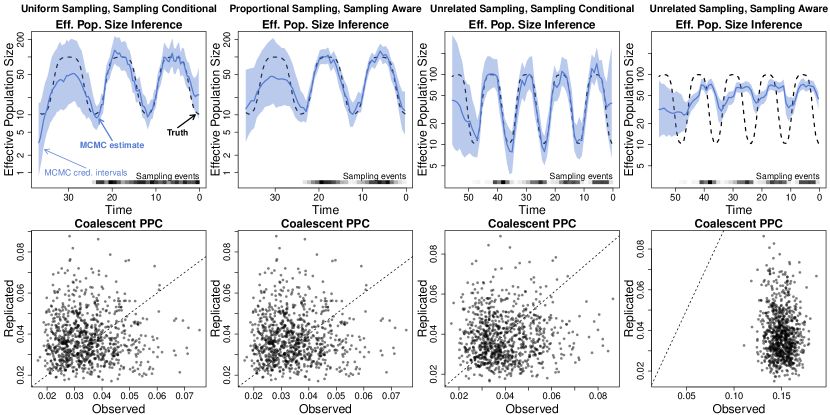
Figure B-1: Effective population size inference and coalescent posterior predictive check for fixed-tree simulations. The dashed black line represents the true effective population trajectory. The solid blue line represents the posterior median effective population trajectory inferred by fixed-tree MCMC and the light blue region represents the corresponding pointwise 95% credible intervals for the effective population trajectory.

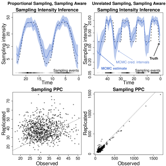
Figure B-2: Sampling intensity inference and sampling time posterior predictive check for fixed-tree simulations. The dashed black line represents the true sampling intensity. The solid blue line represents the posterior median sampling intensity inferred by fixed-tree MCMC, and the light blue region represents the corresponding pointwise 95% credible intervals for the sampling intensity.

Scenario	Sampling Model	Post. Pred. p-val
		Coalescent	Sampling
Uniform	Conditional	0.58	—
Proportional	Aware: $\boldsymbol{\gamma}(t)$	0.59	0.72
Unrelated	Conditional	0.46	—
Unrelated	Aware: $\boldsymbol{\gamma}(t)$	0.00	0.15

Table B-1: Posterior predictive p-values for simulated fixed-tree data.

In our first scenario, we simulate 500 sampling times, distributed according to a uniform distribution between $t=0$ and $t=24$ (weeks), and simulate a genealogy with effective population size $N_{e,10,100,12,0}(t)$. We infer the underlying effective population size trajectory with a sampling-conditional posterior using a Markov chain Monte Carlo (MCMC) method with an elliptical slice sampling transition kernel (ESS) [Murray et al., 2010] as implemented in phylodyn (illustrated in the first row, first column of Figure B-1) We use the MCMC output to generate replicate coalescent data as laid out in Section B.1.3 and calculate our coalescent discrepancy $D_{c}$ for the observed MCMC results as well as for the replicated results. We plot the discrepancy comparison in the second row, first column of Figure B-1, and note that the posterior predictive p-value is 0.58, which is close to 0.5, correctly suggesting that the model is adequate.

We proceed with several additional scenarios. We simulate 514 sampling times between $t=0$ and $t=24$ (weeks), distributed proportionally to the effective population size, with sampling log-intensity $\log[\lambda_{c}(t)]=-0.97+N_{e,10,100,12,0}(t)$. We infer the underlying effective population size trajectory with a sampling-aware posterior (illustrated in the second column of Figure B-1), with sampling time model $\log[\lambda_{s}(t)]=\beta_{0}+\beta_{1}\cdot\boldsymbol{\gamma}(t)$. We calculate the posterior predictive p-value as 0.59, again correctly suggesting adequacy. We also simulate 509 sampling times between $t=0$ and $t=48$ (weeks), distributed proportionally to a piecewise constant function $P(t)$ (illustrated in the second column of Figure B-2) unrelated to the effective population size, with log-sampling intensity $\log[\lambda_{c}(t)]=-1.67+P(t)$. We infer the underlying effective population size trajectory using two different methods. We use the sampling-conditional method (illustrated in the third column of Figure B-1) and the sampling-aware method (illustrated in the fourth column of Figure B-1) with sampling log-intensity $\log[\lambda_{s}(t)]=\beta_{0}+\beta_{1}\cdot\boldsymbol{\gamma}(t)$. The sampling-conditional posterior predictive p-value becomes 0.46, suggesting that this method (which only considers the coalescent model) does produce an adequate estimate of the effective population size trajectory. The sampling-aware posterior predictive p-value becomes zero, suggesting that this method produced a very poor estimate of the effective population size trajectory (very visible in Figure B-1). This is likely due to the sampling time model mistaking fluctuations in sampling intensity for information about the effective population size trajectory, illustrating the importance of model checking when the true sampling model is uncertain.

For our sampling-aware scenarios, we apply our sampling time posterior predictive check as well. Our chi-squared sampling discrepancy $D_{\chi^{2}}$ generates a posterior predictive p-value of 0.72, correctly suggesting a good fit. The unrelated sampling scenario also produces a sampling posterior predictive p-value. We see a relatively low posterior predictive p-value of 0.15, reacting to differences between the true and inferred sampling intensity trajectories.

Sequence Data Inference

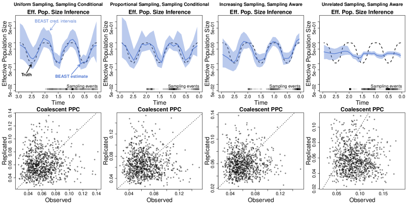
Figure B-3: Effective population size inference and coalescent posterior predictive check for sequence data simulations. The dashed black line represents the true effective population trajectory. The solid blue line represents the posterior median effective population trajectory inferred by BEAST, and the light blue region represents the corresponding pointwise 95% credible intervals for the effective population trajectory.

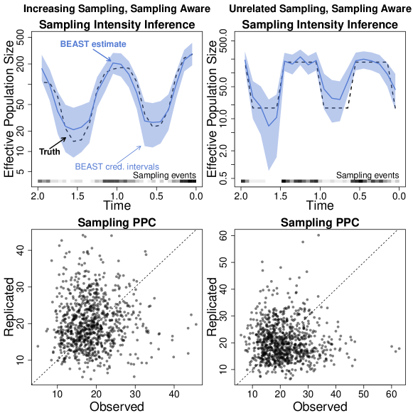
Figure B-4: Sampling intensity inference and sampling time posterior predictive check for sequence data simulations. The dashed black line represents the true sampling intensity. The solid blue line represents the posterior median sampling intensity inferred by BEAST, and the light blue region represents the corresponding pointwise 95% credible intervals for the sampling intensity.

Scenario	Sampling Model	Post. Pred. p-val
		Coalescent	Sampling
Uniform	Conditional	0.51	—
Proportional	Conditional	0.50	—
Increasing	Aware: $\boldsymbol{\gamma}(t)$	0.47	0.56
Unrelated	Aware: $\boldsymbol{\gamma}(t)$	0.17	0.46

Table B-2: Posterior predictive p-values for simulated sequence data.

Now, we expand the scope of our simulation study to be based on simulated sequence alignment data instead of a known genealogy. In this section, all of our examples will be based on an effective population size trajectory of $N_{e,1,10,1,0.5}(t)$, mimicking the trajectory of a seasonal disease as measured in units of years. Similar to the previous section, we generate sampling times and genealogies according to different sampling scenarios and the coalescent, respectively. Given a genealogy, we simulate sequence data using the software SeqGen [Rambaut and Grassly, 1997] using the Jukes-Cantor 1969 [Jukes et al., 1969] substitution model to generate 1500 sites. We set the substitution rate to produce an expected 0.9 mutations per site, in order to produce a sequence alignment with many sites having one mutation and some sites having zero or multiple mutations.

For our first simulation, we distribute 200 sampling times uniformly between $t=0$ and $t=2$ (years). We infer the underlying genealogy and effective population size trajectory using the software BEAST [Suchard et al., 2018] with an elliptical slice sampling transition kernel (ESS) [Murray et al., 2010] as implemented in Section 2, with a sampling-conditional posterior. Finally, we generate replicate genealogies as in the previous section, and we calculate our coalescent discrepancy $D_{c}$ for the observed BEAST results as well as the replicates. In Figure B-3 (first column), we see that the effective population estimate is close to the true trajectory, and when we compare the observed and replicate discrepancies, we calculate a posterior predictive p-value of 0.51, corroborating the model’s adequacy. Next, we distribute 170 sampling times between $t=0$ and $t=2$ (years) with sampling log-intensity $\log[\lambda_{c}(t)]=2.90+N_{e,1,10,1,0.5}(t)$. We infer the underlying genealogy and effective population size trajectory using the sampling-conditional model and calculate discrepancies as above. Note this is a model misspecification applying a sampling-conditional model to a preferential sampling sampling scenario in the style of [Karcher et al., 2016]. Unfortunately, the posterior predictive p-value (0.50) does not detect this mismatch, as the bias effective population size estimate is hard to visually detect in Figure B-3.

In our third scenario, we distribute 199 sampling times between $t=0$ and $t=2$ (years) with increasing sampling log-intensity $\log[\lambda_{c}(t)]=3.35-0.5t+N_{e,1,10,1,0.5}(t)$. We infer as above, but targeting the sampling-aware posterior with sampling log-intensity $\log[\lambda_{s}(t)]=\beta_{0}+\beta_{1}\cdot\boldsymbol{\gamma}(t)$. This is again a misspecification, as the model cannot recover the $-0.5t$ term. However, the posterior predictive check does not clearly detect the mismatch, with a posterior predictive p-value of 0.47. Our sampling posterior predictive check does not detect the misspecification either, with a posterior predictive p-value of 0.56. In our final scenario, we distribute 222 sampling times between $t=0$ and $t=2$ (years) with a sampling log-intensity $\log[\lambda_{c}(t)]=2.84+P^{\prime}(t)$ ($P^{\prime}(t)$ illustrated in Figure B-4, second column) unrelated to the effective population size. We target the sampling-aware posterior, with sampling log-intensity $\log[\lambda_{s}(t)]=\beta_{0}+\beta_{1}\cdot\boldsymbol{\gamma}(t)$. The model reconstructs the effective population size trajectory poorly, and this is successfully reflected in the posterior predictive p-value of 0.17. However, our sampling posterior predictive check does not detect the misspecification, with a posterior predictive p-value of 0.46.

B.2.2 Seasonal Influenza

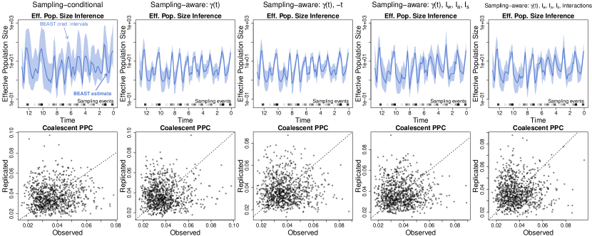
Figure B-5: Effective population size inference and coalescent posterior predictive check for seasonal influenza data. The solid blue line represents the posterior median effective population trajectory inferred by BEAST, and the light blue region represents the corresponding pointwise 95% credible intervals for the effective population trajectory.

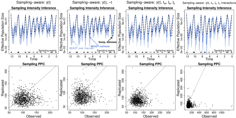
Figure B-6: Sampling intensity inference and sampling time posterior predictive check for seasonal influenza data. The dashed black line represents the true sampling intensity. The solid blue line represents the posterior median sampling intensity inferred by BEAST, and the light blue region represents the corresponding pointwise 95% credible intervals for the sampling intensity.

We apply our posterior predictive check methods to the North American subset of global H3N2 influenza [Zinder et al., 2014]. The data contains 520 sequences aligned to form a multiple sequence alignment with 1698 sites of the hemagglutinin gene. We use the same sequence data BEAST framework as the previous section, choosing four different specific sampling time models. We use a sampling-conditional model with no sampling time model, a simple log-linear sampling time model, and sampling models with different sets of covariates, including $I_{w}(t)=I_{(t\text{ mod }1)\in[0,0.25)}$ as an indicator function for winter, $I_{a}(t)=I_{(t\text{ mod }1)\in[0.25,0.5)}$ as an indicator function for autumn, and $I_{s}(t)=I_{(t\text{ mod }1)\in[0.5,075)}$ as an indicator function for summer.

Figure B-5 shows the inferred effective population size trajectories and coalescent posterior predictive checks for the models. All estimated trajectories follow a similar seasonal trajectory, and the discrepancy comparison suggests that the estimated trajectory produces reasonable results with large posterior predictive p-values (Table B-3). Figure B-6 shows the inferred sampling intensities compared against a nonparametric sampling time-only estimate of the sampling intensity, as well as sampling posterior predictive checks for the four models. The sampling posterior predictive check produces moderate-to-low posterior predictive p-values, suggesting some model inadequacy manifesting in the sampling intensity estimates.

Sampling Model	Post. Pred. p-val
	Coalescent	Sampling
Conditional	0.47	—
Aware: $\boldsymbol{\gamma}(t)$	0.48	0.29
Aware: $\boldsymbol{\gamma}(t),-t$	0.47	0.32
Aware: $\boldsymbol{\gamma}(t),I_{w},I_{a},I_{s}$	0.49	0.16
Aware: $\boldsymbol{\gamma}(t),I_{w},I_{a},I_{s},\{I_{w},I_{a},I_{s}\}\cdot\boldsymbol{\gamma}(t)$	0.49	0.16

Table B-3: Posterior predictive p-values for seasonal influenza data.

B.2.3 Ebola Outbreak

Next, we analyze a subset of sequence data from the recent African Ebola outbreak [Dudas et al., 2017]. We use the same sequence data BEAST framework as the previous section, choosing four different specific sampling time models. We use a sampling-conditional model with no sampling time model, a simple log-linear sampling time model, and several additional sampling-aware models with different sets of covariates.

Figure B-7 shows the inferred effective population size trajectories and coalescent posterior predictive checks for the four models. All estimated trajectories follow a similar effective population size trajectory that visually resembles a typical time trajectory of prevalence or incidence that peaks in Autumn of 2014. The discrepancy comparison suggests that the estimated trajectory produces reasonable results with large posterior predictive p-values (Table B-4). Figure B-9 shows the inferred sampling intensities compared against a nonparametric sampling time-only estimate of the sampling intensity, as well as sampling posterior predictive checks for the four models. The sampling posterior predictive check produces small posterior predictive p-values (Table B-4), suggesting notable model inadequacy manifesting in the sampling intensity estimates.

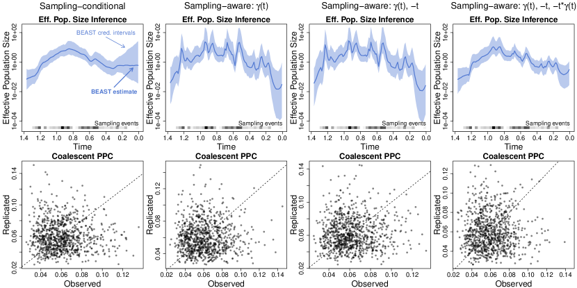
Figure B-7: Effective population size inference and coalescent posterior predictive check for Sierra Leone Ebola data (part 1). The solid blue line represents the posterior median effective population trajectory inferred by BEAST, and the light blue region represents the corresponding pointwise 95% credible intervals for the effective population trajectory.

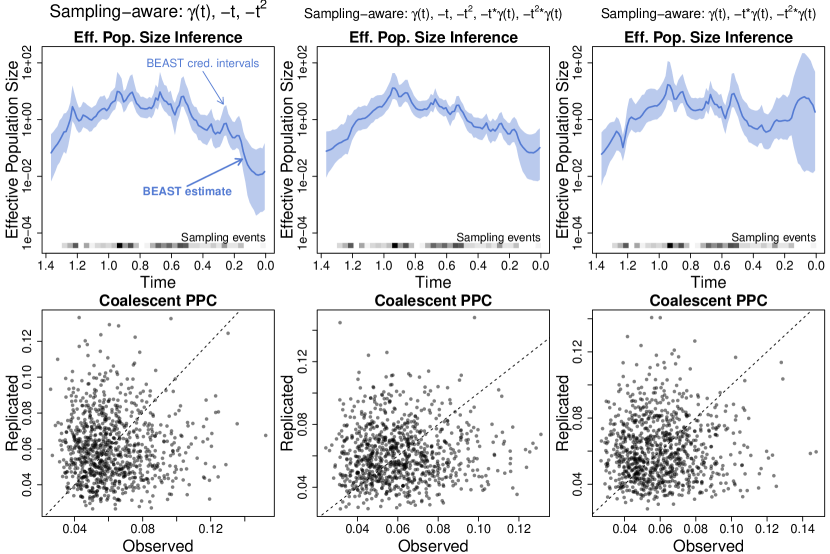
Figure B-8: Effective population size inference and coalescent posterior predictive check for Sierra Leone Ebola data (part 2). The solid blue line represents the posterior median effective population trajectory inferred by BEAST, and the light blue region represents the corresponding pointwise 95% credible intervals for the effective population trajectory.

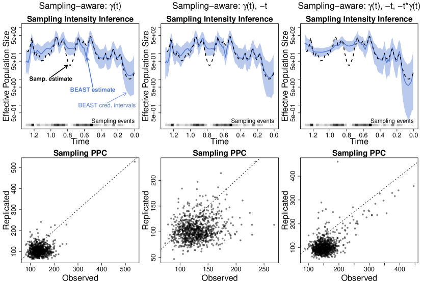
Figure B-9: Sampling intensity inference and sampling time posterior predictive check for Sierra Leone Ebola data (part 1). The dashed black line represents the true sampling intensity. The solid blue line represents the posterior median sampling intensity inferred by BEAST, and the light blue region represents the corresponding pointwise 95% credible intervals for the sampling intensity.

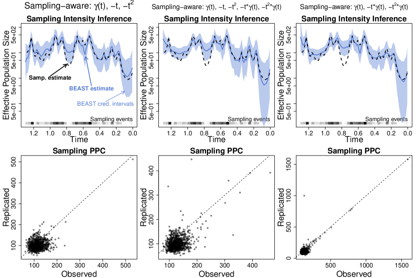
Figure B-10: Sampling intensity inference and sampling time posterior predictive check for Sierra Leone Ebola data (part 2). The dashed black line represents the true sampling intensity. The solid blue line represents the posterior median sampling intensity inferred by BEAST, and the light blue region represents the corresponding pointwise 95% credible intervals for the sampling intensity.

Sampling Model	Post. Pred. p-val
	Coalescent	Sampling
Conditional	0.48	—
Aware: $\boldsymbol{\gamma}(t)$	0.47	0.15
Aware: $\boldsymbol{\gamma}(t),-t$	0.50	0.18
Aware: $\boldsymbol{\gamma}(t),-t,-t\cdot\boldsymbol{\gamma}(t)$	0.50	0.06
Aware: $\boldsymbol{\gamma}(t),-t,-t^{2}$	0.48	0.31
Aware: $\boldsymbol{\gamma}(t),-t,-t^{2},\{-t,-t^{2}\}\cdot\boldsymbol{\gamma}(t)$	0.51	0.17
Aware: $\boldsymbol{\gamma}(t),\{-t,-t^{2}\}\cdot\boldsymbol{\gamma}(t)$	0.51	0.22

Table B-4: Posterior predictive p-values for Sierra Leone Ebola data.

Appendix C Appendix: Ebola incidence data

As we explain in Section 4.3, we compare estimated effective population size trajectories with observed incidence data. We multiplied incidence count by 0.01 — a number determined by trial-and-error, to bring incidence and effective population size to the same scale — and plot effective population size posterior summaries and incidence counts for Sierra Leone and Liberia in Figures C-1 and C-2.

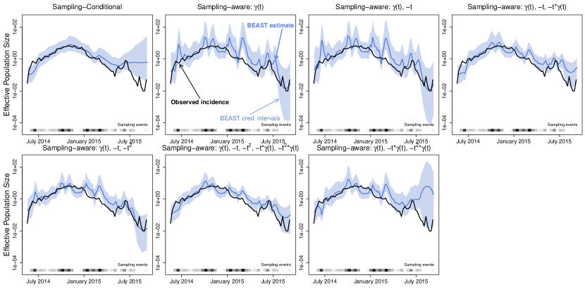
Figure C-1: Comparison of effective population size reconstructions with incidence data in Sierra Leone. The solid blue line represents the posterior median effective population trajectory inferred by BEAST, and the light blue region represents the corresponding pointwise 95% credible intervals for the effective population trajectory. The solid black line shows the observed incidence scaled by a constant so it is on the same scale as the effective population size.

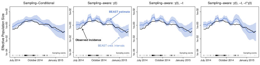
Figure C-2: Comparison of effective population size reconstructions with incidence data in Liberia. See Figure C-1 caption for the legend explanation.

References

- Çinlar [1975] E. Çinlar. Introduction to Stochastic Processes. Prentice-Hall, Inc., Englewood Cliffs, New Jersey, 1975.
- CDC [2010] CDC. The 2009 H1N1 pandemic: Summary highlights, april 2009-april 2010, 2010. URL https://www.cdc.gov/h1n1flu/cdcresponse.htm.
- Drummond et al. [2002] A. J. Drummond, G. K. Nicholls, A. G. Rodrigo, and W. Solomon. Estimating mutation parameters, population history and genealogy simultaneously from temporally spaced sequence data. Genetics, 161(3):1307–1320, 2002.
- Drummond et al. [2005] A. J. Drummond, A. Rambaut, B. Shapiro, and O. G. Pybus. Bayesian coalescent inference of past population dynamics from molecular sequences. Molecular Biology and Evolution, 22(5):1185–1192, 2005.
- Drummond et al. [2003] A.J. Drummond, O.G. Pybus, A. Rambaut, R. Forsberg, and A.G. Rodrigo. Measurably evolving populations. Trends in Ecology & Evolution, 18(9):481–488, 2003.
- Dudas et al. [2017] G. Dudas, L. M. Carvalho, T. Bedford, A. J. Tatem, G. Baele, N. R. Faria, D. J. Park, J. T. Ladner, A. Arias, D. Asogun, et al. Virus genomes reveal factors that spread and sustained the Ebola epidemic. Nature, 544(7650):309–315, 2017.
- Felsenstein [1973] J. Felsenstein. Maximum likelihood and minimum-steps methods for estimating evolutionary trees from data on discrete characters. Systematic Biology, 22(3):240–249, 1973.
- Felsenstein [1981] J. Felsenstein. Evolutionary trees from DNA sequences: a maximum likelihood approach. Journal of Molecular Evolution, 17(6):368–376, 1981.
- Felsenstein and Rodrigo [1999] J. Felsenstein and A. G. Rodrigo. Coalescent Approaches to HIV Population Genetics. In The Evolution of HIV, pages 233–272. Johns Hopkins University Press, 1999. ISBN 9780801861512.
- Frost and Volz [2010] S. D. W. Frost and E. M. Volz. Viral phylodynamics and the search for an ‘effective number of infections’. Philosophical Transactions of the Royal Society B: Biological Sciences, 365(1548):1879–1890, 2010.
- Gelman et al. [1996] Andrew Gelman, Xiao-Li Meng, and Hal Stern. Posterior predictive assessment of model fitness via realized discrepancies. Statistica Sinica, pages 733–760, 1996.
- Gill et al. [2013] M. S. Gill, P. Lemey, N. R. Faria, A. Rambaut, B. Shapiro, and M. A. Suchard. Improving Bayesian population dynamics inference: a coalescent-based model for multiple loci. Molecular Biology and Evolution, 30(3):713–724, 2013.
- Gill et al. [2016] M.S Gill, P. Lemey, S.N. Bennett, R. Biek, and M.A. Suchard. Understanding past population dynamics: Bayesian coalescent-based modeling with covariates. Systematic Biology, 65(6):1041–1056, 2016.
- Griffiths and Tavaré [1994a] R. C Griffiths and S. Tavaré. Ancestral inference in population genetics. Statistical science, pages 307–319, 1994a.
- Griffiths and Tavaré [1994b] R. C. Griffiths and S. Tavaré. Sampling theory for neutral alleles in a varying environment. Philosophical Transactions of the Royal Society of London. Series B: Biological Sciences, 344(1310):403–410, 1994b.
- Hein et al. [2004] J. Hein, M. Schierup, and C. Wiuf. Gene genealogies, variation and evolution: a primer in coalescent theory. Oxford University Press, USA, 2004.
- Heled and Drummond [2008] Joseph Heled and Alexei J Drummond. Bayesian inference of population size history from multiple loci. BMC Evolutionary Biology, 8(1):289, 2008.
- Jukes et al. [1969] T. H. Jukes, C. R. Cantor, H. N. Munro, et al. Evolution of protein molecules. Mammalian protein metabolism, 3(21):132, 1969.
- Karcher et al. [2016] M. D. Karcher, J. A. Palacios, T. Bedford, M. A. Suchard, and V. N. Minin. Quantifying and mitigating the effect of preferential sampling on phylodynamic inference. PLoS Computational Biology, 12:e1004789, 2016.
- Karcher et al. [2017] M.D. Karcher, J.A. Palacios, S. Lan, and V.N. Minin. phylodyn: an R package for phylodynamic simulation and inference. Molecular Ecology Resources, 17(1):96–100, 2017.
- Kingman [1982] J. F. C. Kingman. The coalescent. Stochastic Processes and Their Applications, 13(3):235–248, 1982.
- Lan et al. [2015] S. Lan, J. A. Palacios, M. D. Karcher, V. N. Minin, and B. Shahbaba. An efficient Bayesian inference framework for coalescent-based nonparametric phylodynamics. Bioinformatics, 31:3282–3289, 2015.
- Massey Jr [1951] Frank J Massey Jr. The Kolmogorov-Smirnov test for goodness of fit. Journal of the American statistical Association, 46(253):68–78, 1951.
- Minin et al. [2008] V. N. Minin, E. W. Bloomquist, and M. A. Suchard. Smooth skyride through a rough skyline: Bayesian coalescent-based inference of population dynamics. Molecular Biology and Evolution, 25(7):1459–1471, 2008.
- Murray et al. [2010] I. Murray, R.P. Adams, and D. Mackay. Elliptical slice sampling. In International Conference on Artificial Intelligence and Statistics, pages 541–548, 2010.
- Palacios and Minin [2012] J. A. Palacios and V. N. Minin. Integrated nested Laplace approximation for Bayesian nonparametric phylodynamics. In Proceedings of the Twenty-Eighth International Conference on Uncertainty in Artificial Intelligence, pages 726–735, 2012.
- Palacios and Minin [2013] J. A. Palacios and V. N. Minin. Gaussian process-based Bayesian nonparametric inference of population size trajectories from gene genealogies. Biometrics, 69(1):8–18, 2013.
- Pearson [1900] K. Pearson. On the criterion that a given system of deviations from the probable in the case of a correlated system of variables is such that it can be reasonably supposed to have arisen from random sampling. The London, Edinburgh, and Dublin Philosophical Magazine and Journal of Science, 50(302):157–175, 1900.
- Rambaut and Grassly [1997] A. Rambaut and N. C. Grassly. Seq-gen: an application for the Monte Carlo simulation of DNA sequence evolution along phylogenetic trees. Bioinformatics, 13(3):235–238, 1997.
- Shapiro et al. [2005] B. Shapiro, A. Rambaut, and A.J. Drummond. Choosing appropriate substitution models for the phylogenetic analysis of protein-coding sequences. Molecular Biology and Evolution, 23(1):7–9, 2005.
- Sinharay and Stern [2003] S. Sinharay and H. S. Stern. Posterior predictive model checking in hierarchical models. Journal of Statistical Planning and Inference, 111(1):209–221, 2003.
- Slatkin and Hudson [1991] M. Slatkin and R. R. Hudson. Pairwise comparisons of mitochondrial dna sequences in stable and exponentially growing populations. Genetics, 129(2):555–562, 1991.
- Suchard et al. [2018] Marc A Suchard, Philippe Lemey, Guy Baele, Daniel L Ayres, Alexei J Drummond, and Andrew Rambaut. Bayesian phylogenetic and phylodynamic data integration using BEAST 1.10. Virus Evolution, 4(1):vey016, 2018.
- Volz and Frost [2014] E. M. Volz and S. D. W. Frost. Sampling through time and phylodynamic inference with coalescent and birth–death models. Journal of The Royal Society Interface, 11(101):20140945, 2014.
- Volz et al. [2009] E. M. Volz, S. L. K. Pond, M. J. Ward, A. J. L. Brown, and S. D. W. Frost. Phylodynamics of infectious disease epidemics. Genetics, 2009.
- Wakeley and Sargsyan [2009] J. Wakeley and O. Sargsyan. Extensions of the coalescent effective population size. Genetics, 181(1):341–345, 2009.
- Zinder et al. [2014] D. Zinder, T. Bedford, E. B. Baskerville, R. J. Woods, M. Roy, and M. Pascual. Seasonality in the migration and establishment of H3N2 influenza lineages with epidemic growth and decline. BMC Evolutionary Biology, 14(1):272, 2014.