Step Change Improvement in ADMET Prediction with
PotentialNet Deep Featurization

Abstract

The Absorption, Distribution, Metabolism, Elimination, and Toxicity (ADMET) properties of drug candidates are estimated to account for up to 50% of all clinical trial failures Kennedy (1997); Kola and Landis (2004). Predicting ADMET properties has therefore been of great interest to the cheminformatics and medicinal chemistry communities in recent decades. Traditional cheminformatics approaches, whether the learner is a random forest or a deep neural network, leverage fixed fingerprint feature representations of molecules. In contrast, in this paper, we learn the features most relevant to each chemical task at hand by representing each molecule explicitly as a graph, where each node is an atom and each edge is a bond. By applying graph convolutions to this explicit molecular representation, we achieve, to our knowledge, unprecedented accuracy in prediction of ADMET properties. By challenging our methodology with rigorous cross-validation procedures and prospective analyses, we show that deep featurization better enables molecular predictors to not only interpolate but also extrapolate to new regions of chemical space.

I Introduction

Only about 12% of drug candidates entering human clinical trials ultimately reach FDA approvalKola and Landis (2004). This low success rate stems to a significant degree from issues related to the absorption, distribution, metabolism, elimination, and toxicity (ADMET) properties of a molecule. In turn, ADMET properties are estimated to account for up to 50% of all clinical trial failures Kennedy (1997); Kola and Landis (2004).

Over the past few years, Merck has been heavily invested in leveraging institutional knowledge in an effort to drive hypothesis-driven, model-guided experimentation early in discovery. To that end, in silico models have been established for many of our early screening assay endpoints deemed critical in the design of suitable potential candidates in order to selectively invest available resources in chemical matter having the best possible chance of delivering an efficacious and safe drug candidate in a timely fashion Sherer et al. (2012); Sanders et al. (2017).

Supervised machine learning (ML) is an umbrella term for a family of functional forms and optimization schemes for mapping input features representing input samples to ground truth output labels. The traditional paradigm of ML involves representing training samples as flat vectors of features Hastie, Tibshirani, and Friedman (2009). This featurization step frequently entails domain-specific knowledge. For instance, recent work in protein-ligand binding affinity prediction represents, or featurizes, a protein-ligand co-crystal complex with a flat vector containing properties including number of hydrogen bonds, number of salt bridges, number of ligand rotatable bonds, and floating point measures of such properties as hydrophobic interactions Durrant and McCammon (2011); Ballester and Mitchell (2010); Li et al. (2015).

In the domain of ligand-based QSAR, cheminformaticians have devised a variety of schemes to represent individual molecules as flat vectors of mechanized features. Circular fingerprints Rogers and Hahn (2010) of bond diameter 2, 4, and 6 (ECFP2, ECFP4, ECFP6, respectively) hash local neighborhoods of each atom to bits in a fixed vector. In contrast, atom pair features Carhart, Smith, and Venkataraghavan (1985) denote pairs of atoms in a given molecule, the atom types, and the minimum bond path length that separates the two atoms. In a supervised ML setting, regardless of specific featurization, all such fixed length vector featurizations will be paired with a learning algorithm of choice (e.g., Random Forests, Support Vector MachinesHastie, Tibshirani, and Friedman (2009), multilayer perceptron deep neural networks, i.e. MLP DNN’s Goodfellow et al. (2016)) that will then return a mapping of features to some output assay label of interest.

While circular fingerprints, atom pair features, MACCS keys Durant et al. (2002), and related generic schemes have the potential to supersede the signal present in hand-crafted features, they are still inherently limited by the insuperable inefficiency of projecting a complex multidimensional object onto a single dimension. Whereas graph convolutions win with molecules by exploiting the concept of bond adjacency, two-dimensional convolutions win with images by exploiting pixel adjacency, and recurrent neural networks win by exploiting temporal adjacency, there is no meaning to proximity of bits along either an ECFP or pair descriptor set of molecular features. For instance, considering the pair descriptor framework, an $sp^{3}$ carbon that is five bonds away from an $sp^{2}$ nitrogen might denote the first bit in the feature vector, an $sp^{2}$ oxygen that is two bonds away from an $sp^{3}$ nitrogen might denote the very next bit in the same feature vector, and an $sp^{3}$ carbon that is four bonds away from an $sp^{2}$ nitrogen might denote the hundredth bit in the feature vector. Put in descriptor language, a feature like “CX3sp3-04-NX1sp2” is conceptually similar to “CX20sp3-04-NX2sp2”, but the descriptors are treated as fully unrelated in descriptor-based QSAR while graph convolutional approaches could separate the “element” component from the “hybridization” component and both from the “bond distance” component. The conceptual proximity between qualitatively similar descriptors is weakened by the arbitrary arrangement of bits in the featurization process and therefore must be “re-learned” by the supervised machine learning algorithm of choice.

To both compare and contrast chemical ML on fixed vector descriptors with chemical deep learning on graph features, we write out a multilayer perceptron (MLP) and a graph convolutional neural network (GCNN) side-by-side (Figure 1). In Figure 1, each molecule is represented either by a flat vector $x$ for the MLP or by both an $N_{atoms}\times N_{atoms}$ adjacency matrix $A$ and an $N_{atoms}\times f_{in}$ per-atom feature matrix $X$ for the GCNN. The GCNN begins with $K$ graph convolutional layers. It then proceeds to a graph gather operation that sums over the per-atom features in the last graph convolutional hidden layer: $x^{(NN)}=\sum_{atoms}H^{(K)}$, where the differentiable $x^{(NN)}$, by analogy to the fixed input $x$ of the MLP, is a flat vector graph convolutional fingerprint for the entire molecule, and $H^{(K)}_{i}$ is the feature map at the $K^{\prime}th$ graph convolutional layer for atom $i$. The final layers of the GCNN are identical in form to the hidden layers of the MLP. The difference, therefore, between the MLP and the GCNN lies in the fact that $x$ for MLP is a fixed vector of molecular fingerprints, whereas $x^{(NN)}$ of the GCNN is an end-to-end differentiable fingerprint vector: the features are learned in the graph convolution layers.

Another noteworthy parallel arises between the MLP hidden layers and the GCNN graph convolutional layers. Whereas the first MLP layer maps $h^{(1)}=ReLU(W^{(1)}\cdot x)$, the GCNN inserts the adjacency matrix $A$ between $W$ and atom feature matrix $X$: $H^{(1)}=ReLU(W^{(1)}\cdot A\cdot X)$. Note that, while the feature maps $X,H^{(1)},...,H^{(K)}$ change at each layer of a GCNN, the adjacency matrix $A$ is a constant to be re-used at each layer. Therefore, in a recursive manner, a given atom is passed information about other atoms succesively further in bond path length at each graph convolutional layer.

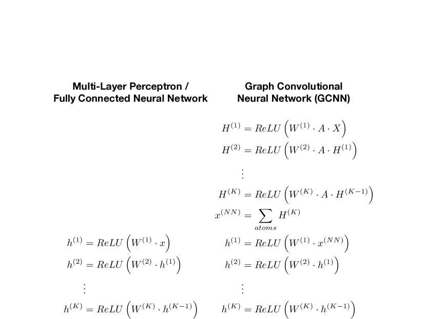
Figure 1: Comparison of algorithms for multilayer perceptron versus graph convolution.

Since the advent of the basic graph convolutional neural network, a spate of new approachesKearnes et al. (2016); Kipf and Welling (2016); Li et al. (2016); Gilmer et al. (2017); Feinberg et al. have improved upon the elementary graph convolutional layers expressed in Figure 1. Here, we train neural networks based on the PotentialNet Feinberg et al. family of graph convolutions.

$$h^{(1)}_{i} =GRU\left(x_{i},\sum^{N_{\text{et}}}_{e}\sum_{j\in N^{(e)}(v_{i})}NN^{(e)}(x_{j})\right)$$ (1)

$$\vdots$$

$$h^{(K)}_{i} =GRU\left(h^{(b_{K-1})}_{i},\sum^{N_{\text{et}}}_{e}\sum_{j\in N^{(e)}(v_{i})}NN^{(e)}(h^{(b_{K-1})}_{j})\right)$$

$$h^{(NN)} =\sigma\left(i(h^{(K)},x)\right)\odot\left(j(h^{(K)})\right)$$

$$h^{(FC_{0})} =\sum^{N_{Lig}}_{j=1}h^{(NN)}_{j}$$

$$h^{(FC_{1})} =ReLU\left(W^{(FC_{1})}h^{(FC_{0})}\right)$$

$$\vdots$$

$$h^{(FC_{K})} =W^{(FC_{K})}h^{(FC_{K-1})}$$

where $h_{i}^{(k)}$ represents the feature map for $atom_{i}$ at graph convolutional layer $k$; $i$, $j$, and $NN$ are neural networks, $N_{Lig}$ is the number of ligand atoms, $\{W\}$ are weight matrices for different layers. The GRU is a Gated Recurrent Unit which affords a more efficient passing of information to an atom from its neighbors. In this way, whereas one might view the standard GCNN displayed in Figure 1 as more analogous to learnable and more efficient ECFP featurization, one might view the PotentialNet layers in Equation 1 as being more analogous to a learnable and more efficient pair descriptorCarhart, Smith, and Venkataraghavan (1985) featurization.

In this paper, we conduct a direct comparison of the current state-of-the-art algorithm similar to those used by many major pharmaceutical companies – random forests based on atom pair descriptors – with PotentialNet (Equation 1). We trained ML models on thirty-one chemical datasets describing results of various ADMET assays – ranging from physicochemical properties to animal-based PK properties – and compared results of random forests with those of PotentialNet on held out test sets chosen by two different cross-validation strategies (further details on PotentialNet training are included in Methods). In addition, we ascertain the capacity of our trained models to generalize to assays conducted outside of our institution by downloading datasets from the scholarly literature and conducting further performance comparisons. Finally, we conduct a prospective comparison of prediction accuracy of Random Forests and PotentialNet on assay data of new chemical entities recorded well after all model parameters were frozen in place.

II Results

The primary purpose of supervised machine learning is to train computer models to make accurate predictions about samples that have not been seen before in the learning process. In the discipline of computer vision, the ability to interpolate between training samples is often sufficient for real-world applications. Such is not the case in the field of medicinal chemistry. When a chemist is tasked with generating new molecular entities to selectively modulate a given biological target, they must invent chemical matter that is fundamentally different than previously known materials. This need stems from both scientific and practical concerns; every biological target is different and likely requires heretofore nonexistent chemical matter, and the patent system demands that, to garner protection, new chemical entities must be not only useful but also novel and sufficiently different from currently existing molecules.

Cross-validation is a subtle yet critical component of any ML initiative. In the absence of the ability to gather prospective data, it is standard practice in ML to divide one’s retrospectively available training data into three disjoint subsets: train, valid, and test (though it is only strictly necessary that the test set be disjoint from the others). It is well known that cross-validation strategies typically used in the vision or natural language domains, like random splitting, significantly over-estimate the generalization and extrapolation ability of machine learning methodsSheridan (2013). As a result, we deploy two train-test splits that, compared to random splitting, are at once more challenging and also more accurately reflect the real world task of drug discovery. First, we split all datasets temporally, training on molecules assayed before the earliest $date_{i}$, selecting models based on performance on molecules assayed between $date_{i}$ and intermediate $date_{j}$, and evaluating the final model on held-out molecules assayed after the latest $date_{j}$. Such temporal splitting is meant to parallel the types of progressions that typically occur in lead optimization programs as well as reflect broader changes in the medicinal chemistry field.

In addition to temporal splitting, we introduce an additional cross-validation strategy in which we both divide train, valid, and test sets temporally and add the following challenge: (1) removal of molecules with molecular weight greater than $500\frac{g}{mol}$ from the training and validation sets and (2) inclusion of only molecules with molecular weight greater than or equal to $600\frac{g}{mol}$ from the test set. We denote this as temporal plus molecular weight split (Figure 2).

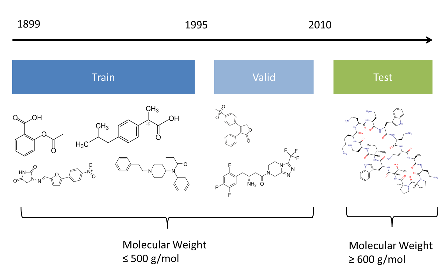
Figure 2: Temporal plus Molecular Weight Split. In this rigorous cross-validation procedure, one trains and selects models based on older, smaller molecules, with the resultant best model (according to the validation set score) being evaluated a single time on a held out test set on newer, larger molecules. Specifically, the train and validation sets are comprised only of molecules below a certain molecular weight threshold and synthesized before a certain date, whereas the test set is comprised only of molecules above a certain molecular weight threshold and synthesized after a certain date.

II.1 Temporal Split

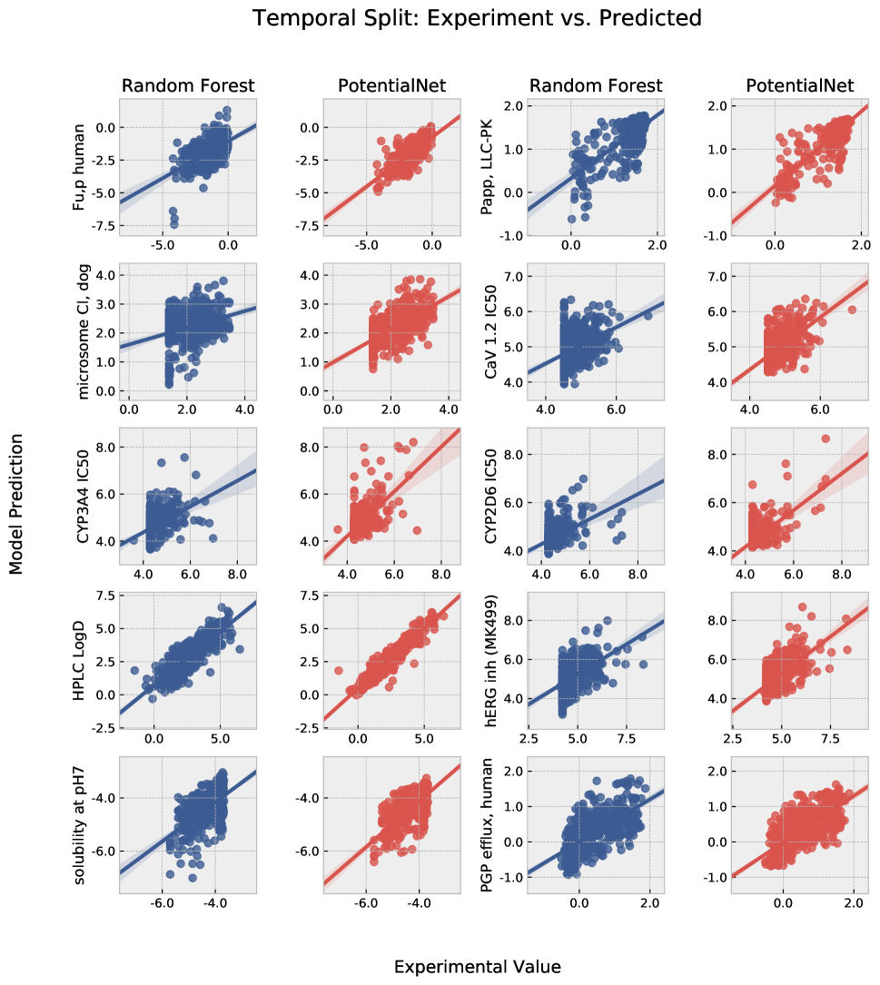
Figure 8: Temporal Split: Scatter plots of predictions by PotentialNet and by Random Forest vs. Experiment for Several Assays

In aggregate, PotentialNet achieves a $64\%$ average improvement and a $52\%$ median improvement in $R^{2}$ over Random Forests across all thirty-one reported datasets (Figure 3, Table 1, Table 6). The mean $R^{2}$ over the various test datasets is $0.30$ for Random Forests and $0.44$ for PotentialNet, corresponding to a mean $\overline{\Delta R^{2}}\left(PotentialNet-RandomForest\right)=0.15$. Among the assays for which PotentialNet offers the most improvement (Figure 8) are plasma protein binding (fraction unbound for both human, $\Delta R^{2}=0.34$ and rat, $\Delta R^{2}=0.38$), microsomal clearance (human: $\Delta R^{2}=0.21$, dog: $\Delta R^{2}=0.26$, rat: $\Delta R^{2}=0.22$), CYP3A4 Inhibition ($\Delta R^{2}=0.22$), logD ($\Delta R^{2}=0.18$), and passive membrane absorption ($\Delta R^{2}=0.18$). Meanwhile, assays HPLC EPSA and rat clearance, which account for two of the thirty-one assays, show no statistically significant difference. All $R^{2}$ values are reported with confidence intervals computed according to ref Walters (2018).

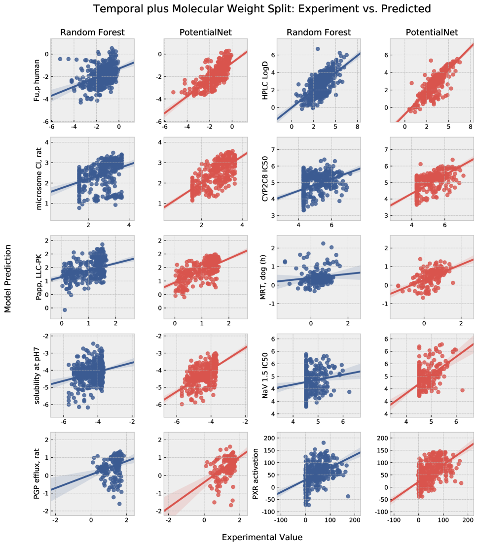
Figure 9: Temporal plus Molecular Weight Split: Scatter plots of predictions by PotentialNet and by Random Forest vs. Experiment for Several Assays

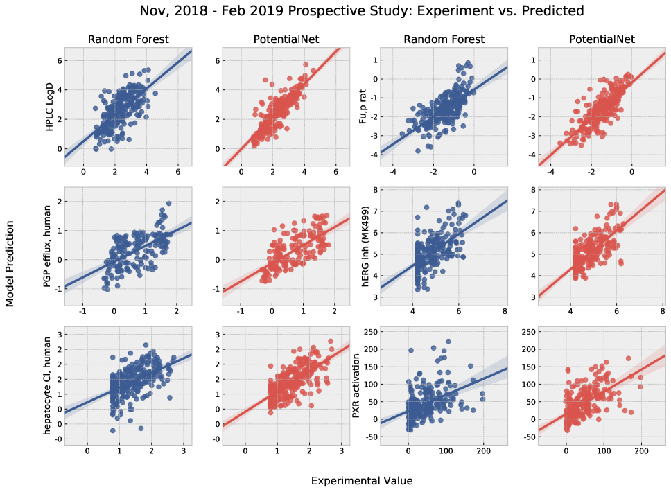
Figure 10: Nov, 2018 - Feb, 2019 Prospective Data: Scatter plots of predictions by PotentialNet and by Random Forest vs. Experiment for Several Assays. All models were trained on data and compounds registered up through August, 2018 and tested prospectively on data and compounds registered in Nov, 2018 - Feb, 2019

In addition to improvements in $R^{2}$, for both cross-validation schemes discussed, we note that the slope of the linear regression line between predicted and experimental data is, on average, closer to unity for PotentialNet than it is for Random Forests. This difference is qualitatively notable in Figure 8. A corollary, which is also illustrated by Figures 8, 9, and 10, is that PotentialNet DNN’s perform noticeably better than Random Forest in predicting the correct range of values for a given prediction task. At our institution, this deficiency of RF is in part rectified by ex post facto prediction rescaling, which in part recovers the slope but makes no difference in $R^{2}$.

The commercially available molecules for which PotentialNet achieved the greatest improvement in prediction versus Random Forests are displayed in Table 4. An example of a molecule on which Random Forest renders a more accurate prediction is shown in Table 5.

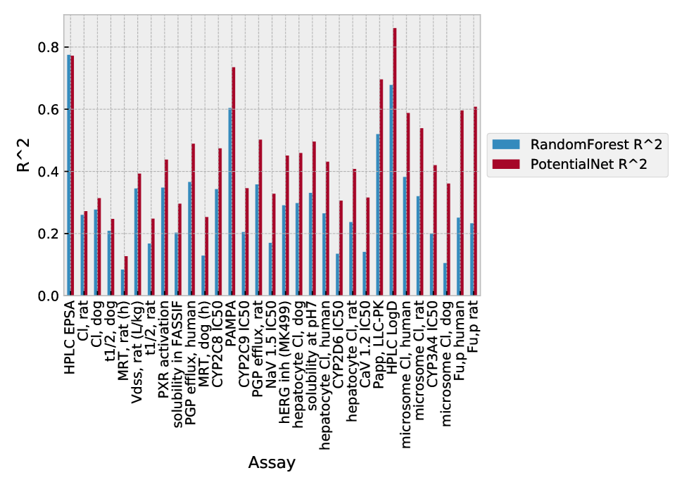
Figure 3: Temporal Split: Performance of PotentialNet versus Random Forest for All Assays

II.2 Temporal plus Molecular Weight Split

We then investigated the cross-validation setting where data was both (a) split temporally and (b) molecules with $MW>500\frac{g}{mol}$ were removed from the training set while only molecules with $MW>600\frac{g}{mol}$ were retained in the test set (Figure 2). In aggregate, PotentialNet achieves a $153\%$ median improvement in $R^{2}$ over Random Forests across all twenty-nine reported datasets (Table 2, Figure 4). The mean $R^{2}$ over the various test datasets is $0.12$ for Random Forests and $0.28$ for PotentialNet, corresponding to a mean $\Delta R^{2}\left(PotentialNet-RandomForest\right)=0.16$. The assays for which PotentialNet offers the most improvement (Figure 9) are plasma protein binding (fraction unbound for both human, $\Delta R^{2}=0.38$ and rat, $\Delta R^{2}=0.47$), microsomal clearance (human: $\Delta R^{2}=0.29$, dog: $\Delta R^{2}=0.19$, rat: $\Delta R^{2}=0.37$), CYP2C8 Inhibition ($\Delta R^{2}=0.25$), logD ($\Delta R^{2}=0.25$), and passive membrane absorption ($\Delta R^{2}=0.28$). Meanwhile, human hepatocyte clearance, CYP2D6 Inhibition, rat and dog clearance, dog halflife, human PGP (efflux), rat MRT, and rat volume of distribution exhibit no statistically significant difference in model predictivity ($\frac{8}{29}$ of all datasets), with only rat hepatocyte clearance being predicted less well for PotentialNet as compared to Random Forests. It should be noted that the quantity of molecules in the test sets are smaller in temporal plus MW split as compared to temporal only split, and therefore, it is accordingly more difficult to reach statistically significant differences in $R^{2}$ (S.I. Table 4).

The commercially available molecules for which PotentialNet achieved the greatest improvement in prediction versus Random Forests are displayed in Table 9. It is intriguing that the same molecule undergoes the greatest improvement for both Human Fraction Unbound as well as CYP2D6 Inhibition.

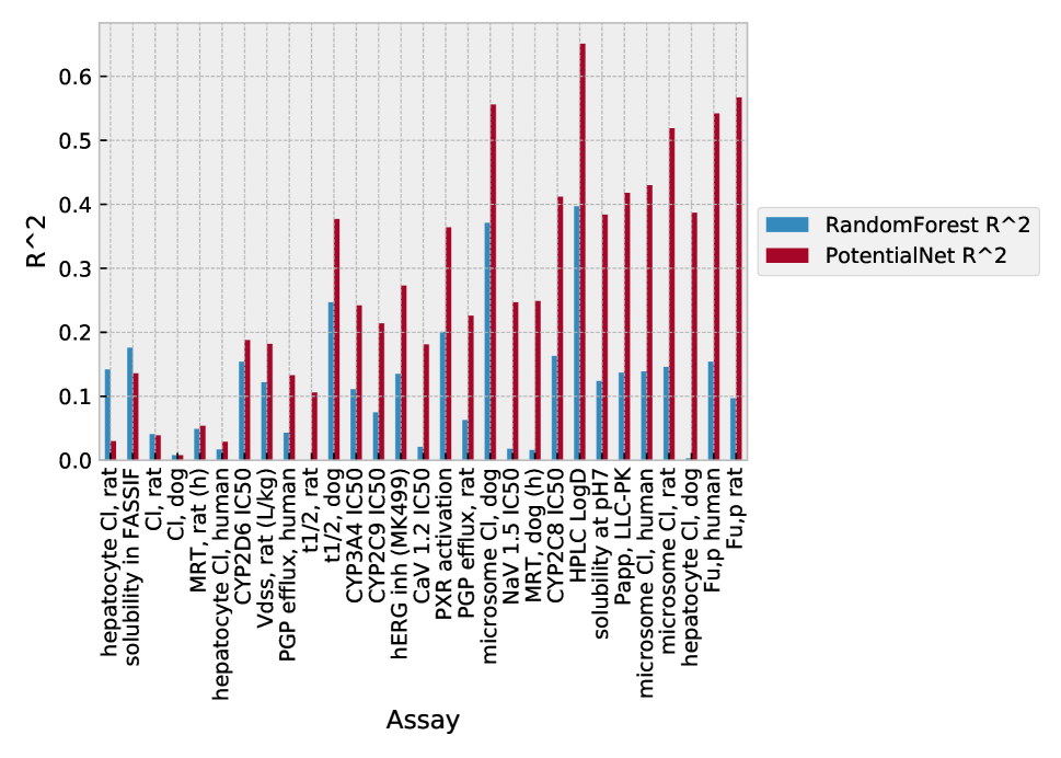
Figure 4: Temporal plus Molecular Weight Split: Performance of PotentialNet versus Random Forest for All Assays

As previous works have noted Xu et al. (2017), multitask style training (cf. Methods) can boost – or, less charitably, inflate – the performance of neural networks by sharing information between the training molecules of one task and the test molecules of another task, especially if the activities are in some way correlated. Another advantage of the Temporal plus Molecular Weight cross-validation approach is that it mitigates hemorrhaging of information between assay datasets. By introducing a minimum $100\frac{g}{mol}$ molecular weight gap between train and test molecules, it is not only impossible for train molecules in one task to appear as test molecules for another task, but it also circumscribes the similarity of any given task’s training set to any given other task’s test set. We further investigate the relative effect of multitask versus single task training in Supplementary Table 2. However, even in cases where there is similarity or even identity between training molecules of one assay and test molecules of another assay, in the practice of chemical machine learning, this may in fact be desirable in cases. For instance, if less expensive, cell-free assays, like solubility, have a strong correlation with a more expensive endpoint, like dog mean residence time, it would be an attractive property of multitask learning if solubility data on molecules in a preexisting database could inform more accurate predictions of the animal mean residence time of untested, similar molecules.

II.3 Held out data from literature

To further ascertain the generalization capacity of our models, we obtained data from scholarly literature. In particular, we obtained data on macrocyclic compounds for passive membrane permeability and logD from ref Over et al. (2016). We observed a statistically significant increase in performance (Table 10) for both passive membrane permeability ($\Delta R^{2}\left(PotentialNet-RandomForest\right)=0.23$) and logD ($\Delta R^{2}\left(PotentialNet-RandomForest\right)=0.21$). The four molecules for which PotentialNet exhibits the greatest improvement in predictive accuracy over Random Forests are shown in Table 11.

The second molecule in Table 11 is experimentally quite permeable, which PotentialNet correctly identifies but Random Forests severely underestimates. Note that the aliphatic tertiary amine would likely be protonated and therefore charged at physiologic pH. The proximity of an ether oxygen may “protect” the charge, increasing the ability to passively diffuse through lipid bilayers. Because of the relative efficiency with which information traverses bonds in a graph convolution as opposed to the fixed pair features that are provided to the random forest, it is intuitively straightforward for a graph neural network to learn the “atom type” of a high pKa nitrogen in spatial proximity to an electron rich oxygen, whereas pair features would rigidly specify an aliphatic nitrogen three bonds away from an aliphatic oxygen.

II.4 Feature Interpretation

Feature interpretation remains a fledgling discipline in many areas of deep learning. We posit a simple method here to probe a given graph convolutional neural network to expose intuitive reasons driving that network’s decision-making process. Recall that the basic graph convolutional update is $h^{(1)}=ReLU\left(W^{(1)}\cdot A\cdot X\right)$. For a given molecule $\hat{x}$ with predicted property $\hat{y}$, we can use the backpropagation algorithm to determine the gradient, or partial derivative per feature, on the input. We define the feature-wise importance $Imp(atom_{i})$ of $atom_{i}$ as:

$$Imp(atom_{i})=\sum_{j=0}^{(f_{in})}\frac{\partial NN(A,X)}{\partial X_{ij}}$$ (2)

where $f_{in}$ is the initial number of features per atom (number of columns of $X$) and $X_{ij}$ is the $j^{\prime}th$ feature of $atom_{i}$.

By a related metric, we can posit the substructure, or functional group, of size $S$ atoms of a molecule that has the greatest impact on the graph convolutional neural network’s prediction by:

$$argmax_{\text{subgraph G'}}\sum_{atom_{j}\in G^{\prime}}Imp(atom_{j})$$ (3)

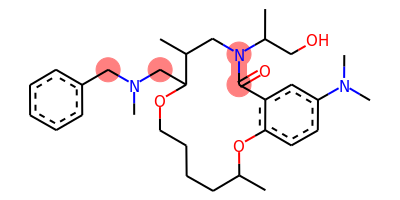
(a) Individually Most Important Atoms

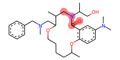
(b) Most Important Substructure

Figure 11: Feature interpretation for macrocycle in ref Over et al. (2016)

The above comprises a plausible route for feature interpretation in graph convolutional neural networks. While a rigorous evaluation of this approach will remain the subject of future work, we illustrate how it would function with a large molecule example. Let us reexamine the case of the molecule in Table 11 that is correctly identified by PotentialNet as membrane permeable (and misidentified by Random Forests as impermeable). Intriguingly, the feature importance score (Equation 2) points to the two carbons neighboring the tertiary amine nitrogen, and the amide carbon and nitrogen as the four most important atoms for determining permeability (Figure 11a, Equation 2). The importance of the tertiary amine adjacent atoms certainly correlates with chemical intuition. Meanwhile, the amide group is seen as important by both individual per-atom gradient ranking as well as by maximal substructure importance (Figure 11b, Equation 3). The interpretation of the amide’s high importance is less obvious, though several studiesRezai et al. (2006); Hickey et al. (2016) have examined the influence of macrocycle amides and permeability. For instance, it has been proposedRezai et al. (2006) that amide groups in the main ring of macrocycles stabilize conformations that enable intramolecular hydrogen bond formation, thereby reducing the effective polar surface area of the molecule. It is possible that the graph neural network is learning a correlation between macrocyclic amides and reduced polar surface area.

II.5 Prospective Study

II.5.1 Overall Prospective Performance on Nov, 2018 - Feb, 2019 Data

In September, 2018, we froze the parameters of Random Forest and PotentialNet models trained on all available assay data recorded internally at Merck up to the end of August, 2018. After approximately two months had elapsed after the registration of the last training data point, we evaluated the performance of those a priori frozen models on new experimental assay data gathered on compounds registered between November, 2018 and the end of February, 2019. Not only does this constitute a prospective analysis, but a particularly rigorous one in which there is a two month gap between training data collection and prospective model evaluation, further challenging the generalization capacity of the trained models. For statistical power, we chose to evaluate performance on all assays for which at least ten compounds were experimentally tested the period Nov, 2018 - Feb, 2019. Over these twenty-seven assays, Random Forest achieved a median $R^{2}$ of 0.32, whereas PotentialNet achieved a median $R^{2}$ of 0.43 for a median $\Delta R^{2}=0.10$ (Table 3). Performance of each assay can be found in Figure 5 and Table 8, and scatter plots of predicted versus experimental values for several assays can be found in Figure 10. While it makes no difference in $R^{2}$, we have chosen to scale the values predicted by both Random Forests and by PotentialNet to match the mean and standard deviation of the distribution of assay data in the training set to more faithfully reflect how these models would be used practically in an active pharmaceutical project setting.

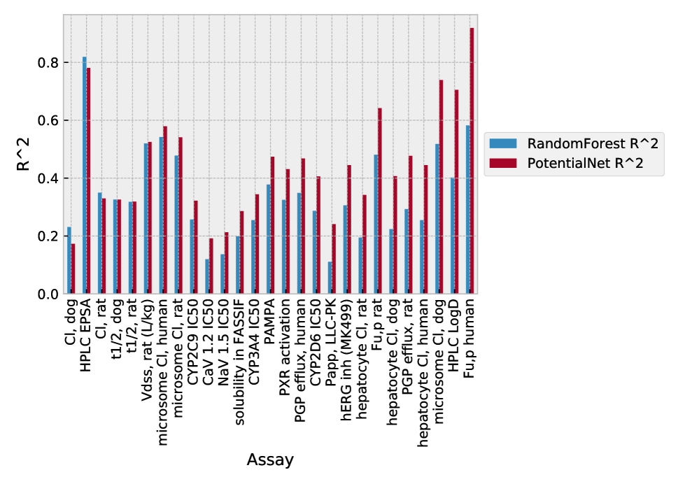
Figure 5: Prospective Study. All model parameters for both PotentialNet and Random Forests were frozen in August, 2018. Subsequently, performance of both models was compared for new assay data collected on compounds registered from Nov, 2018 - Feb, 2019.

II.5.2 Performance on Two Specific Projects

To assess performance on individual projects, we applied the August, 2018, models to prediction of rat plasma fraction unbound on two currently active lead optimization projects at Merck. The results (Figure 6) suggest that the performance on the individual projects are similar to the temporal split and temporal + molecular weight split results.

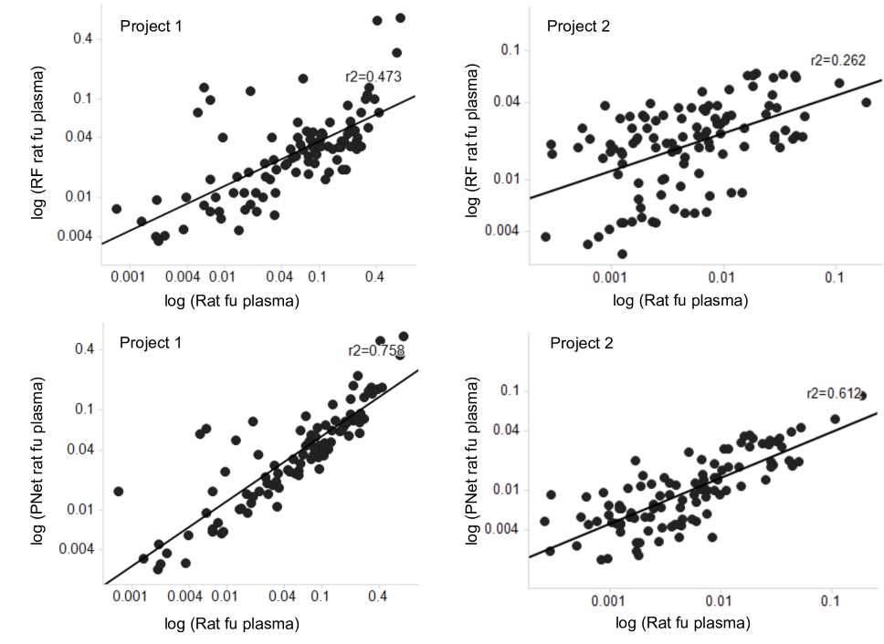
Figure 6: Prospective prediction of rat fraction unbound in plasma (rat fu,p) in two active projects using random forest models (top row) and potential net models (bottom row), for compounds experimentally tested between September and December 2018. Data for Project 1 and Project 2 is for 97 and 123 compounds, respectively.

III Discussion

Preclinical drug discovery is a critica, and often rate-limiting stage of the broader pharmaceutical development pipeline. While estimates vary between studies, recent analyses estimate the capitalized cost of preclinical discovery per FDA-approved drug as anywhere between $89 Million and $834 Million DiMasi, Hansen, and Grabowski (2003); Morgan et al. (2011); Paul et al. (2010). The multi-objective optimization among potency and ADMET properties, which can entail vexing trade-offs, is a critical bottleneck in preclinical discovery Wager et al. (2010); Segall et al. (2011). More accurate prediction of ADMET endpoints can both prevent exploration of undesirable chemical space as well as facilitate access to desirable regions of chemical space, thereby making preclinical discovery not only more efficient but perhaps more productive as well.

To assess if a modern graph convolutional neural network Feinberg et al. succeeds in more accurately predicting ADMET endpoints, we conducted a rigorous performance comparison between GCNN and the previous state-of-the-art random forest based on cheminformatic features. With an emphasis on rigor, we included a total of thirty-one assay datasets in our analysis, employed two cross-validation splits (temporal split Sheridan (2013) and a combined temporal plus molecular weight split), and made predictions on a publicly available held-out test set. Finally, we made prospective predictions with both random forests and with PotentialNet and then compared with experimental results.

Encouragingly, statistical improvements were observed in each of the four aforementioned validation settings. In the temporal split setting, across thirty-one tasks, Random Forests achieved a mean $R^{2}$ of 0.30, whereas PotentialNet achieved a mean $R^{2}$ of 0.44 (Table 1). In the temporal plus molecular weight split setting – where only older smaller molecules were included in the training set while only newer larger molecules included in the test set – across twenty-nine tasks, Random Forests achieved a mean $R^{2}$ of 0.12, whereas PotentialNet achieved a mean $R^{2}$ of 0.28 (Table 2). In the final pseudo-prospective validation setting, we assessed the ability of pre-trained Random Forests and pre-trained PotentialNet models to predict passive membrane permeability and logD on an experimental dataset on macrocycles obtained from the literatureOver et al. (2016). In this setting, for passive membrane permeability, Random Forests achieved an $R^{2}$ of 0.15 whereas PotentialNet achieved an $R^{2}$ of 0.38; for logD, Random Forests achieved an $R^{2}$ of 0.39 whereas PotentialNet achieved an $R^{2}$ of 0.60 (Table 9).

While the three described retrospective investigations are more rigorous than random splitting and are meant to more faithfully reflect the generalization capacity of a model in the practical real world of pharmaceutical chemistry, we also believe that prospective validation is important whenever the resources are available to do so. To this end, we made predictions on twenty-three assays, each of which contained measurements for new chemical entities synthesized and evaluated after November, 2018 (the last data point for model training was collected in August, 2018). In aggregate, there is a mean $\Delta R^{2}$ of $0.10$ of PotentialNet over Random Forests. This improvement in accuracy in a future and relatively constrained time window is largely consistent with that prognosticated by the retrospective temporal split study and is encouraging for the utility of deep featurization in a predictive capacity for drug discovery.

Historically, as a discipline, machine learning arose from statistical learning, and a key line of inquiry in statistics involves extricating potentially confounding variables. Compared with random forests, we introduce several algorithmic changes at once: use of neural network instead of random forest; use of graph convolution as a neural network architecture based on a graph adjacency and feature matrices as input rather than either RF or MLP based on flat 1D features; and use of a variant of multitask learning rather than single task learning. How much of the performance gain accrued by PotentialNet can be attributed to each of the aforementioned changes? To investigate, we conducted an algorithm ablation study to compare performance contributions (Supplementary Tables 2 and 6; we also include xgboost for additional comparison). It is reasonable to contend that one should solely compare random forest with single task neural networks since the former is incapable of jointly learning on several assay datasets simultaneously. However, one of the intuitive advantages of a GCNN over either RF or MLP is that a GCNN can learn the atomic interaction features relevant to the prediction task at hand. Therefore, we aver that the most reflective comparison is to apply best practices that are accessible by each technique. Not only can graph convolutions learn the features, but adding different molecules from different tasks allows networks to learn more accurately both through the effect of task correlation and learning richer features by incorporating a greater area of chemical space.

While we are restricted with respect to the compounds in our training data that we can disclose, we can share select publicly disclosed compounds that happened to have been tested in the assays discussed in this work. Table 4 lists commercially available compounds for which PotentialNet’s predictions are most improved compared to Random Forests’ predictions in the temporal split setting. For example, the first compound, Methyl 4-chloro-2-iodobenzoate, has an experimental logD of 3.88, Random Forests predicts logD to be 2.26, and PotentialNet predicts logD to be 3.70. Neural network interpretation remains a discipline in its infancy and therefore renders it challenging to pinpoint exactly which aspect of either the initial featurization or the network enables PotentialNet to properly estimate the logD while Random Forests significantly underestimates it. As a hypothetical analysis, pair features would include such terms as “carbonyl oxygen that is three bonds away from ether carbon,” “carbonyl oxygen that is four bonds away from aromatic iodine,” and “carbonyl oxygen that is six bonds away from an aromatic chlorine.” There is no sense that it is the same carbonyl carbon that has all of these properties. In stark contrast, by recursively propagating information, a graph convolution would confer a single, dense “atom type” on the carbonyl oxygen that would reflect its identity as a halogenated benzaldehyde oxygen.

More accurate prediction of ADMET endpoints can be a torchPaszke et al. (2017)light guiding creative medicinal chemists as they explore uncharted chemical space en route to the optimal molecule. The results delineated in this paper demonstrate that deep-feature learning with graph convolutions can systematically and often quite significantly outperform random forests based on fixed fingerprints. We therefore deem it advisable for pharmaceutical scientists to consider integrating deep learning in general and graph convolutions in particular in their modeling pipelines.

Methods

PotentialNet (Equation 1) Feinberg et al. neural networks were constructed and trained with PyTorch Paszke et al. (2017). Multilayer perceptron (MLP) neural networks were trained with the assistance of the MIX library that is internal to Merck (more details below). Following previous works Ramsundar et al. (2015), we make extensive use of multitask learning to train our PotentialNet models. We modified the standard multitask framework to save different models for each task on the epoch at which performance was best for that specific task on the validation set (Figure 7). In that way, we employ an approach that draws on elements of both single and multitask learning. Custom Python code was used based on RDKit rdk and OEChem oec with frequent use of NumPy Walt, Colbert, and Varoquaux (2011) and SciPy Jones et al. (01). Networks were trained on chemical element, formal charge, hybridization, aromaticity, and the total numbers of bonds, hydrogens (total and implicit), and radical electrons. Random forest were implemented using both scikit-learn Pedregosa et al. (2011) and MIX; all sklearn-trained random forests models were trained with $500$ trees and $\sqrt{n_{features}}$ per tree; xgboost models were trained using MIX.

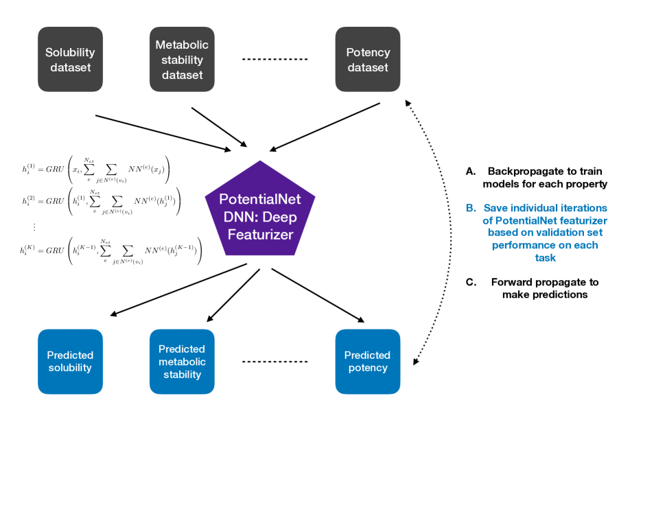
Figure 7: Multitask framework for PotentialNet training

QSAR Descriptors: Chemical descriptors, termed “APDP” used in this study for random forests, xgboost, and MLP DNN’s are listed as follows. All descriptors are used in frequency form, i.e. we use the number of occurrences in a molecule and not just the binary presence or absence. APDP denotes the union of AP, the original “atom pair” descriptor from ref Carhart, Smith, and Venkataraghavan (1985), and DP descriptors (“Donor acceptor Pair”), called “BP” in ref. Kearsley et al. (1996). Such APDP descriptors are used in most of Merck’s QSAR studies and in Merck’s production QSAR. Both descriptors are of the form: “Atom $type_{i}$ – (distance in bonds) – Atom $type_{j}$”

For AP, atom type includes the element, number of nonhydrogen neighbors, and number of pi electrons; it is very specific. For DP, atom type is one of seven (cation, anion, neutral donor, neutral acceptor, polar, hydrophobe, and other); it contains a more generic description of chemistry.

QSAR methods: All methods are used in regression mode, i.e. both input activities and predictions are floating-point numbers. All appropriate descriptors are used in the models, i.e. no feature selection is done. When random forests are not trained with scikit-learn, they are trained with the Merck MIX library that in turn calls the R module RandomForest Breiman et al. (2011), which encodes the original method of ref. Breiman (2001) and first applied to QSAR in ref.Svetnik et al. (2003). The default settings are 100 trees, nodesize=5, mtry=M/3 where M is the number of unique descriptors.

MLP Deep neural networks (DNN): We use Python-based code obtained from the Kaggle contest and described in ref Ma et al. (2015). We use parameters slightly different than the “standard set” described in that paper: Two intermediate layers of 1000 and 500 neurons with 25% dropout rate and 75 training epochs. The above change is made for the purposes of more time-efficient calculation. The accuracy of prediction is very similar to that of the standard set.

xgboost: Extreme Gradient Boosting method published in ref Chen and Guestrin (2016). In this paper, we are using a set of standard parameters from Merck’s subsequent study using this method Sheridan et al. (2016).

IV Tables

Table 1: Aggregate performance: Temporal Split

Metric	Value
Mean RandomForest R^2	0.30
Mean PotentialNet R^2	0.44
Median RandomForest R^2	0.27
Median PotentialNet R^2	0.43
Mean Absolute R^2 Improvement	0.15
Mean Percentage R^2 Improvement	64%
Median Absolute R^2 Improvement	0.16
Median Percentage R^2 Improvement	52%

Table 2: Aggregate Statistics: Temporal plus Molecular Weight Split

Metric	Value
Mean RandomForest R^2	0.12
Mean PotentialNet R^2	0.28
Median RandomForest R^2	0.12
Median PotentialNet R^2	0.25
Mean Absolute R^2 Improvement	0.16
Mean Percentage R^2 Improvement	1477%
Median Absolute R^2 Improvement	0.16
Median Percentage R^2 Improvement	153%

Table 3: Aggregate performance: Prospective

Metric	Value
Mean RandomForest R^2	0.34
Mean PotentialNet R^2	0.45
Median RandomForest R^2	0.32
Median PotentialNet R^2	0.43
Mean Absolute R^2 Improvement	0.10
Mean Percentage R^2 Improvement	37%
Median Absolute R^2 Improvement	0.10
Median Percentage R^2 Improvement	35%

Table 4: Temporal Split: Commercially Available Molecules for which performance improvement of PotentialNet with graph features over Random Forest with pair features is greatest

Molecule	Property	Exp.	RandomForest	PotentialNet	SMILES
	logD	3.88	2.26	3.70	COC(=O)c1ccc(cc1I)Cl
	logD	-0.61	1.58	0.59	COc1ccc(c(c1F)C(=O)N)F
	Human Fraction Unbound	-0.06	-1.30	-0.45	Cc1c(nc[nH]1) CSCCN/C(=N/C#N)/NC
	Human Fraction Unbound	-2.95	-2.24	-3.07	C[C@@H]([C@@H](Cc1ccc(cc1)Cl) c2cccc(c2)C#N)NC(=O)C(C) (C)Oc3ccc(cn3)C(F)(F)F
	CYP3A4 Inhibition	6.14	4.61	5.54	Cc1cc(n[nH]1)CN(C)c2ncc (c(n2)C3CC3)c4ccncc4
	hERG Inhibition	6.62	5.17	5.80	CCOC(=O)CCNc1cc(nc(n1) c2ccccn2)N3CCc4ccccc4CC3

Table 5: Temporal Split: Example of molecule predicted more accurately by Random Forests than by PotentialNet

Molecule	Property	Exp.	RandomForest	PotentialNet	SMILES
	Human Fraction Unbound	-1.51	-1.55	1.86	Cc1cc(no1)NC(=O) Nc2cc(c(cc2OC)OC)Cl

Table 6: Performance: Temporal Split

Dataset	RandomForest R^2	RandomForest R^2, 95% CI	PotentialNet R^2	PotentialNet R^2, 95% CI	Absolute Improvement	Percentage Improvement
HPLC EPSA	0.775	(0.76, 0.789)	0.772	(0.757, 0.786)	-0.003	-0.340
Cl, rat	0.260	(0.25, 0.271)	0.272	(0.262, 0.282)	0.011	4.360
Cl, dog	0.277	(0.258, 0.295)	0.314	(0.296, 0.333)	0.038	13.579
t1/2, dog	0.209	(0.192, 0.225)	0.247	(0.23, 0.264)	0.038	18.455
MRT, rat (h)	0.084	(0.075, 0.093)	0.127	(0.117, 0.138)	0.044	52.333
Vdss, rat (L/kg)	0.345	(0.335, 0.356)	0.393	(0.383, 0.403)	0.048	13.769
t1/2, rat	0.168	(0.16, 0.177)	0.248	(0.239, 0.258)	0.080	47.625
PXR activation	0.348	(0.342, 0.353)	0.438	(0.432, 0.443)	0.090	25.933
solubility in FASSIF	0.203	(0.197, 0.208)	0.296	(0.291, 0.302)	0.094	46.178
PGP efflux, human	0.366	(0.35, 0.382)	0.489	(0.474, 0.503)	0.123	33.572
MRT, dog (h)	0.129	(0.112, 0.147)	0.253	(0.231, 0.274)	0.124	96.050
CYP2C8 IC50	0.343	(0.331, 0.355)	0.474	(0.462, 0.485)	0.130	38.029
PAMPA	0.604	(0.553, 0.651)	0.735	(0.697, 0.77)	0.131	21.752
CYP2C9 IC50	0.205	(0.2, 0.21)	0.346	(0.341, 0.352)	0.141	68.728
PGP efflux, rat	0.358	(0.341, 0.374)	0.502	(0.487, 0.517)	0.145	40.497
NaV 1.5 IC50	0.170	(0.164, 0.177)	0.328	(0.321, 0.336)	0.158	92.688
hERG inh (MK499)	0.291	(0.286, 0.295)	0.451	(0.447, 0.456)	0.161	55.306
hepatocyte Cl, dog	0.298	(0.266, 0.329)	0.459	(0.429, 0.489)	0.162	54.326
solubility at pH7	0.331	(0.327, 0.335)	0.496	(0.493, 0.5)	0.165	49.843
hepatocyte Cl, human	0.265	(0.252, 0.279)	0.431	(0.417, 0.444)	0.165	62.323
CYP2D6 IC50	0.135	(0.131, 0.14)	0.306	(0.3, 0.312)	0.171	126.063
hepatocyte Cl, rat	0.237	(0.223, 0.251)	0.408	(0.394, 0.422)	0.171	71.951
CaV 1.2 IC50	0.141	(0.135, 0.147)	0.316	(0.31, 0.323)	0.175	124.278
Papp, LLC-PK	0.520	(0.509, 0.532)	0.696	(0.688, 0.704)	0.176	33.781
HPLC logD	0.678	(0.67, 0.686)	0.861	(0.857, 0.865)	0.183	26.984
microsome Cl, human	0.382	(0.369, 0.394)	0.588	(0.578, 0.598)	0.206	53.992
microsome Cl, rat	0.320	(0.307, 0.333)	0.539	(0.528, 0.551)	0.219	68.500
CYP3A4 IC50	0.200	(0.194, 0.205)	0.420	(0.415, 0.426)	0.221	110.634
microsome Cl, dog	0.105	(0.076, 0.137)	0.361	(0.32, 0.402)	0.257	245.523
Fu,p human	0.251	(0.233, 0.27)	0.596	(0.58, 0.611)	0.344	136.910
Fu,p rat	0.233	(0.221, 0.245)	0.608	(0.598, 0.618)	0.375	161.049

Table 7: Performance: Temporal plus Molecular Weight Split

Dataset	RandomForest R^2	RandomForest R^2, 95% CI	PotentialNet R^2	PotentialNet R^2, 95% CI	Absolute Improvement	Percentage Improvement
hepatocyte Cl, rat	0.142	(0.087, 0.206)	0.030	(0.007, 0.068)	-0.112	-78.891
solubility in FASSIF	0.176	(0.158, 0.194)	0.136	(0.12, 0.153)	-0.040	-22.804
Cl, rat	0.041	(0.025, 0.061)	0.039	(0.023, 0.059)	-0.002	-5.284
Cl, dog	0.008	(0.0, 0.037)	0.008	(0.0, 0.037)	-0.000	-0.281
MRT, rat (h)	0.049	(0.028, 0.074)	0.054	(0.032, 0.08)	0.005	10.590
hepatocyte Cl, human	0.017	(0.003, 0.044)	0.029	(0.008, 0.062)	0.012	67.114
CYP2D6 IC50	0.154	(0.134, 0.175)	0.188	(0.166, 0.21)	0.034	21.943
Vdss, rat (L/kg)	0.122	(0.095, 0.153)	0.182	(0.15, 0.216)	0.060	48.745
PGP efflux, human	0.043	(0.008, 0.101)	0.133	(0.066, 0.215)	0.091	212.901
t1/2, rat	0.000	(0.001, 0.004)	0.106	(0.081, 0.134)	0.106	23708.598
t1/2, dog	0.247	(0.176, 0.321)	0.377	(0.302, 0.451)	0.131	52.942
CYP3A4 IC50	0.111	(0.093, 0.129)	0.242	(0.219, 0.265)	0.131	118.507
CYP2C9 IC50	0.075	(0.061, 0.092)	0.214	(0.192, 0.236)	0.138	182.877
hERG inh (MK499)	0.135	(0.123, 0.148)	0.273	(0.258, 0.289)	0.138	102.122
CaV 1.2 IC50	0.021	(0.013, 0.031)	0.181	(0.159, 0.204)	0.160	767.023
PXR activation	0.201	(0.18, 0.223)	0.364	(0.341, 0.387)	0.163	80.830
PGP efflux, rat	0.063	(0.018, 0.132)	0.226	(0.14, 0.32)	0.163	256.734
microsome Cl, dog	0.371	(0.193, 0.544)	0.556	(0.385, 0.695)	0.185	49.751
NaV 1.5 IC50	0.018	(0.01, 0.028)	0.247	(0.222, 0.273)	0.229	1279.873
MRT, dog (h)	0.016	(0.0, 0.062)	0.249	(0.159, 0.346)	0.233	1416.502
CYP2C8 IC50	0.163	(0.116, 0.213)	0.412	(0.357, 0.466)	0.250	153.437
HPLC logD	0.397	(0.354, 0.439)	0.651	(0.618, 0.682)	0.254	63.935
solubility at pH7	0.124	(0.11, 0.138)	0.384	(0.367, 0.402)	0.261	210.535
Papp, LLC-PK	0.137	(0.088, 0.194)	0.418	(0.354, 0.479)	0.280	204.100
microsome Cl, human	0.139	(0.089, 0.196)	0.430	(0.366, 0.491)	0.291	208.433
microsome Cl, rat	0.146	(0.094, 0.205)	0.519	(0.457, 0.577)	0.373	255.865
hepatocyte Cl, dog	0.003	(0.012, 0.047)	0.387	(0.259, 0.509)	0.384	12724.229
Fu,p human	0.154	(0.11, 0.202)	0.542	(0.493, 0.587)	0.387	251.270
Fu,p rat	0.097	(0.065, 0.134)	0.567	(0.526, 0.606)	0.470	486.274

Table 8: Performance: Prospective Split

Dataset	RandomForest R^2	RandomForest R^2, 95% CI	PotentialNet R^2	PotentialNet R^2, 95% CI	Absolute Improvement	Percentage Improvement
Cl, dog	0.231	(0.163, 0.304)	0.173	(0.111, 0.242)	-0.058	-25.162
HPLC EPSA	0.819	(0.806, 0.831)	0.781	(0.765, 0.795)	-0.039	-4.710
Cl, rat	0.350	(0.317, 0.384)	0.330	(0.297, 0.363)	-0.020	-5.770
t1/2, dog	0.326	(0.257, 0.396)	0.326	(0.257, 0.395)	-0.001	-0.162
t1/2, rat	0.318	(0.285, 0.351)	0.319	(0.286, 0.352)	0.001	0.215
Vdss, rat (L/kg)	0.520	(0.49, 0.55)	0.525	(0.494, 0.554)	0.004	0.846
microsome Cl, human	0.542	(0.503, 0.579)	0.579	(0.542, 0.614)	0.037	6.878
microsome Cl, rat	0.478	(0.436, 0.519)	0.541	(0.501, 0.579)	0.063	13.069
CYP2C9 IC50	0.257	(0.232, 0.282)	0.322	(0.296, 0.347)	0.065	25.396
CaV 1.2 IC50	0.120	(0.103, 0.138)	0.192	(0.172, 0.213)	0.072	59.540
NaV 1.5 IC50	0.137	(0.119, 0.155)	0.213	(0.192, 0.234)	0.076	55.582
solubility in FASSIF	0.199	(0.188, 0.21)	0.286	(0.274, 0.298)	0.087	43.823
CYP3A4 IC50	0.255	(0.236, 0.274)	0.344	(0.325, 0.364)	0.089	35.108
PAMPA	0.378	(0.305, 0.45)	0.474	(0.403, 0.541)	0.096	25.487
PXR activation	0.325	(0.308, 0.342)	0.431	(0.414, 0.448)	0.106	32.608
PGP efflux, human	0.349	(0.252, 0.446)	0.468	(0.372, 0.557)	0.119	33.934
CYP2D6 IC50	0.287	(0.261, 0.313)	0.406	(0.38, 0.432)	0.120	41.735
Papp, LLC-PK	0.111	(0.066, 0.164)	0.241	(0.18, 0.304)	0.129	116.526
hERG inh (MK499)	0.306	(0.286, 0.325)	0.445	(0.425, 0.464)	0.139	45.555
hepatocyte Cl, rat	0.195	(0.161, 0.231)	0.342	(0.305, 0.38)	0.147	75.254
Fu,p rat	0.481	(0.45, 0.511)	0.642	(0.617, 0.666)	0.161	33.522
hepatocyte Cl, dog	0.224	(0.15, 0.304)	0.407	(0.326, 0.486)	0.183	81.705
PGP efflux, rat	0.293	(0.076, 0.532)	0.477	(0.234, 0.681)	0.185	63.129
hepatocyte Cl, human	0.255	(0.22, 0.29)	0.445	(0.411, 0.479)	0.190	74.741
microsome Cl, dog	0.518	(0.136, 0.794)	0.739	(0.42, 0.899)	0.221	42.766
HPLC logD	0.402	(0.39, 0.413)	0.705	(0.697, 0.712)	0.303	75.503
Fu,p human	0.582	(0.3, 0.78)	0.919	(0.832, 0.962)	0.337	57.903

Table 9: Temporal plus Molecular Weight Split: Commercially Available Molecules for which performance improvement of PotentialNet with graph features over Random Forest with pair features is greatest

Molecule	Property	Exp.	RandomForest	PotentialNet	SMILES
	Rat Fraction Unbound	-0.85	-2.17	-1.09	c1cc(cc(c1)F)c2cn (nn2)[C@H]3[C@H] ([C@H](O[C@H] ([C@@H]3O)S[C@H] 4[C@@H]([C@H] ([C@H]([C@H](O4)CO)O)n5cc (nn5)c6cccc(c6)F)O)CO)O
	Human Fraction Unbound	-1.17	-2.15	-1.60	C[C@H](Cn1cnc2c1ncnc2N) OCP(=O)(N[C@@H] (C)C(=O)OCc3ccccc3) N[C@@H](C)C(=O)OCc4ccccc4
	logD	4.55	3.02	4.43	Cc1cc(cc(c1) Nc2nccc(n2) c3cn(nn3)Cc4ccc (cc4)OC)c5cnc(s5)C6 (CCC(CC6)C(=O)OC(C)(C)C)O
	CYP2D6 Inhibition	4.30	4.95	4.53	C[C@H](Cn1cnc2c1ncnc2N) OCP(=O)(N[C@@H](C)C (=O)OCc3ccccc3)N[C@@H] (C)C(=O)OCc4ccccc4

Table 10: Performance on Held Out Data from LiteratureOver et al. (2016)

Property	RandomForest $R^{2}$	PotentialNet $R^{2}$
Papp	0.150 (0.081, 0.232)	0.381 (0.292, 0.468)
logD	0.394 (0.305, 0.480)	0.603 (0.528, 0.670)

Table 11: LiteratureOver et al. (2016) Molecules for which performance improvement of PotentialNet with graph features over Random Forest with pair features is greatest

Molecule	Property	Exp.	RandomForest	PotentialNet	SMILES
	Papp	2.33	74.75	4.90	CO[C@H]1CC[C@H]2CCOc3ccc (cc3C(=O)N(C)CCCC(=O)N(C)C[C@@H]1O2)C#N
	Papp	74.34	21.51	52.42	C[C@@H(CO)N1C[C@@H(C[C@@H(CN(C)Cc2ccccc2) OCCCC[C@@H(C)Oc3ccc(cc3C1=O)N(C)C
	logD	-0.70	1.93	0.34	C[C@H](CO)N1C[C@H](C)[C@H] (CN(C)S(=O)(=O)C)OCc2cnnn2CCCC1=O
	logD	4.70	2.63	3.74	COc1ccc(CN(C)C[C@H]2OCCCC[C@H]C)Oc3ccc(NS(=O) (=O)c4ccc(Cl)cc4)cc3C(=O)N(C[C@H]2C)[C@@H](C)CO)cc1

V Figures

V.1 Performance of models trained on Merck data on held out literature macrocycle data

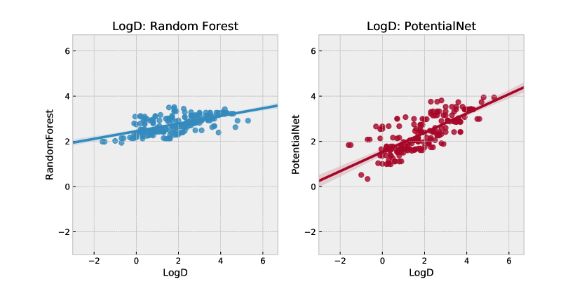
Figure 12: Scatter plots of predictions by models pre-trained on Merck data with both PotentialNet and Random Forest vs. Experiment for logD Measurements on Macrocycles in ref Over et al. (2016)

References

Supplemental Figures

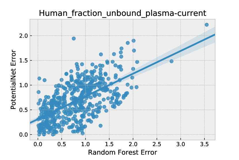
Figure S1: Temporal plus Molecular Weight split: Scatter plot of errors for two models: ABS(PotentialNet - Experiment) vs. ABS(Random Forest - Experiment) for Fu,p human

Figure S2: Plot of $R^{2}$ versus test set size for all datasets for temporal split. Train and test set sizes for each assay for temporal split can be found in SI Figure 7. Test set size is a qualitatively weak predictor of performance for a deep learning model.

Table 1: Temporal plus Molecular Weight Split: Aggregate Performance Across all Datasets while only retaining molecules with $MW>700\frac{g}{mol}$ in the test set

	0
Mean RandomForest R^2	0.091
Mean PotentialNet R^2	0.189
Median RandomForest R^2	0.063
Median PotentialNet R^2	0.178
Mean Absolute R^2 Improvement	0.098
Mean Percentage R^2 Improvement	318.335
Median Absolute R^2 Improvement	0.089
Median Percentage R^2 Improvement	131.795

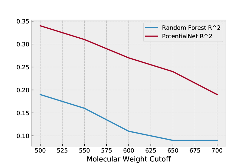
Figure S3: Temporal plus Molecular Weight split for different molecular weight cutoffs. For example, $550$ on the abscissa refers to cross-validation split where only molecules with molecular weight $>550\frac{g}{mol}$ are retained in the test set. For each cross-validation split listed on the abscissa, only molecules with molecular weight $<500\frac{g}{mol}$ are retained in the training and validation sets. Therefore, as one moves right along the abscissa, the train-test split becomes more difficult for the machine learner since the gap in molecular weight between train and test molecules becomes larger, forcing the model to do more extrapolation. While performance of both PotentialNet and Random Forests steadily degrades the larger the gap in MW between train and test molecules, PotentialNet also retains an advantage for each Temporal plus Molecular Weight split examined. Median $R^{2}$ figures are reported over all assays for which there were at least 100 molecules in the test set for a MW cutoff of $700\frac{g}{mol}$.

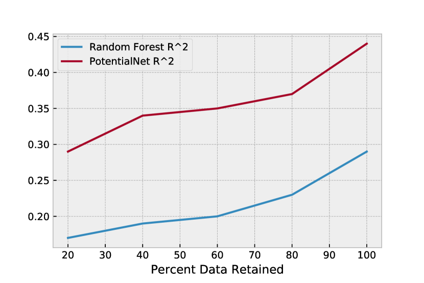
Figure S4: At its core, supervised ML revolves around finding patterns in past data to make predictions on future data. An immediate corollary to this notion is the question of how much past data is needed to make accurate predictions on future data? Here, we performed a training data ablation study. For each of the assay datasets, we temporally removed different proportions of the training and validation data while leaving test data unchanged. For instance, at 60% data retained on the abscissa, we removed 40% of the training and validation data points that were temporally or chronologically latest. Therefore, this is equivalent to introducing a time gap between the last training and validation data point and the earliest test data point. Clearly, temporally removing training and validation data systematically diminishes performance of both random forests and of PotentialNet. Nevertheless, the advantage of PotentialNet versus Random Forests in terms of predictive performance remains qualitatively similar regardless of quantity of data removed. It is intriguing that the signal increase from 80% to 100% is greater than that of 60% to 80%; perhaps this reflects how the most similar ligands to those in the test set are most likely to be temporally adjacent as well.

Table 2: Results on Temporal plus Molecular Weight Split with Random Forests (MIX and Scikit Learn), xgboost, single task multilayer perceptron DNN, single task PotentialNet DNN, and multitask PotentialNet DNN. All results reported with Pearson $R^{2}$

	RF: MIX	RF: sklearn	xgboost	MLP DNN	PotentialNet SingleTask	PotentialNet MultiTask
Rat_fraction_unbound_plasma-current	0.012	0.097	0.054	0.483	0.583	0.567
Ca_Na_Ion_Channel_NaV_1.5_Inhibition	0.012	0.018	0.000	0.235	0.235	0.247
LOGD	0.405	0.397	0.494	0.593	0.749	0.651
CLint_Human_hepatocyte	0.001	0.017	0.000	0.149	0.102	0.029
CYP_Inhibition_3A4	0.084	0.111	0.087	0.158	0.228	0.242
PXR_activation	0.089	0.201	0.037	0.354	0.343	0.364
CYP_Inhibition_2D6	0.024	0.154	0.093	0.154	0.136	0.188
3A4	0.370	0.419	0.262	0.447	0.503	0.588
CLint_Human_microsome	0.202	0.139	0.258	0.174	0.274	0.430
CLint_Rat_hepatocyte	0.035	0.150	0.047	0.070	0.236	0.033
Human_fraction_unbound_plasma-current	0.139	0.154	0.146	0.248	0.418	0.542
MK499	0.053	0.073	0.041	0.093	0.170	0.234
Volume_of_Distribution_Rat	0.130	0.121	0.006	0.059	0.249	0.181
Halflife_Rat	0.016	0.000	0.091	0.035	0.030	0.104
Halflife_Dog	0.016	0.248	0.268	0.195	0.428	0.377
CLint_Dog_hepatocyte	0.087	0.003	0.048	0.064	0.491	0.387
dog_MRT	0.042	0.020	0.000	0.003	0.047	0.255
CLint_Dog_microsome	0.036	0.371	0.346	0.388	0.493	0.556
Absorption_Papp	0.181	0.137	0.064	0.119	0.333	0.418
Clearance_Dog	0.006	0.008	0.001	0.010	0.084	0.008
Ca_Na_Ion_Channel_CaV_1.2_Inhibition	0.017	0.021	0.001	0.114	0.191	0.181
CYP_Inhibition_2C8	0.063	0.163	0.031	0.238	0.358	0.412
Clearance_Rat	0.065	0.041	0.015	0.275	0.014	0.039
CLint_Rat_microsome	0.201	0.146	0.259	0.155	0.362	0.519
CYP_TDI_3A4_Ratio	0.001	0.000	0.026	0.108	0.121	0.099

Table 3: Median $\Delta R^{2}$ over Random Forests for different ML model types on temporal plus MW split.

	0
(RF: sklearn) - (RF: MIX)	0.006
(xgboost) - (RF: MIX)	-0.001
(MLP DNN) - (RF: MIX)	0.097
(PotentialNet, SingleTask) - (RF: MIX)	0.152
(PotentialNet, MultiTask) - (RF: MIX)	0.218

Table 4: Number of molecules in train and test sets for Temporal plus Molecular Weight split

	n_train_mols	n_test_mols
3A4	24904	855
Absorption_Papp	22043	387
CLint_Dog_hepatocyte	2419	100
CLint_Dog_microsome	1381	50
CLint_Human_hepatocyte	15503	416
CLint_Human_microsome	22839	387
CLint_Rat_hepatocyte	14744	316
CLint_Rat_microsome	22065	364
CYP_Inhibition_2C8	19149	524
CYP_Inhibition_2C9	104095	2903
CYP_Inhibition_2D6	103901	2845
CYP_Inhibition_3A4	103189	2883
CYP_TDI_3A4_Ratio	17387	352
Ca_Na_Ion_Channel_CaV_1.2_Inhibition	60305	2656
Ca_Na_Ion_Channel_NaV_1.5_Inhibition	56964	2308
Clearance_Dog	10085	239
Clearance_Rat	28563	1211
Halflife_Dog	11125	282
Halflife_Rat	31768	1332
Human_fraction_unbound_plasma-current	10114	559
LOGD	27840	856
MK499	26466	892
PGP_Human_1uM	16116	192
PGP_Rat_1uM	14907	179
PXR_activation	104203	3004
Rat_MRT	17958	898
Rat_fraction_unbound_plasma-current	20111	714
SOLY_7	221036	5129
Solubility_Fassif	118524	4008
Volume_of_Distribution_Rat	28821	1216
dog_MRT	6830	173
hERG_MK499	180285	6513

Table 5: Number of molecules in train and test sets for Prospective Study

	n_train_mol	n_test_mol
CYP2C9 IC50	206932	2483
CYP2D6 IC50	206565	2333
CYP3A4 IC50	204801	4121
CaV 1.2 IC50	135403	3304
Cl, dog	18875	295
Cl, rat	60190	1451
Fu,p human	17852	21
Fu,p rat	38583	1494
HPLC EPSA	8169	1844
HPLC logD	48914	11280
NaV 1.5 IC50	128359	3356
PAMPA	1700	300
PGP efflux, human	26104	169
PGP efflux, rat	23402	29
PXR activation	208309	5350
Papp, LLC-PK	40131	390
Vdss, rat (L/kg)	60307	1451
hERG inh (MK499)	340680	4011
hepatocyte Cl, dog	6474	243
hepatocyte Cl, human	33251	1249
hepatocyte Cl, rat	30511	1133
microsome Cl, dog	3826	13
microsome Cl, human	41922	849
microsome Cl, rat	39351	824
solubility in FASSIF	212259	10690
t1/2, dog	20720	332
t1/2, rat	66766	1490

Table 6: Results on Temporal Split with Random Forests (sklearn implementation), single task PotentialNet DNN, and multitask PotentialNet DNN. All results reported with Pearson $R^{2}$

	Random Forest R^2	PotentialNet, SingleTask	PotentialNet, MultiTask
3A4	0.450	0.630	0.658
Absorption_Papp	0.520	0.641	0.696
CLint_Dog_hepatocyte	0.298	0.378	0.459
CLint_Dog_microsome	0.105	0.119	0.361
CLint_Human_hepatocyte	0.265	0.390	0.431
CLint_Human_microsome	0.382	0.553	0.588
CLint_Rat_hepatocyte	0.237	0.354	0.408
CLint_Rat_microsome	0.320	0.500	0.539
CYP_Inhibition_2C8	0.343	0.391	0.474
CYP_Inhibition_2C9	0.205	0.342	0.346
CYP_Inhibition_2D6	0.135	0.291	0.306
CYP_Inhibition_3A4	0.200	0.404	0.420
CYP_TDI_3A4_Ratio	0.032	0.025	0.032
Ca_Na_Ion_Channel_CaV_1.2_Inhibition	0.141	0.277	0.316
Ca_Na_Ion_Channel_NaV_1.5_Inhibition	0.170	0.288	0.328
Clearance_Dog	0.277	0.289	0.314
Clearance_Rat	0.260	0.275	0.272
EPSA	0.775	0.758	0.772
Halflife_Dog	0.209	0.201	0.247
Halflife_Rat	0.168	0.218	0.248
Human_fraction_unbound_plasma-current	0.251	0.445	0.596
LOGD	0.678	0.850	0.861
MK499	0.288	0.375	0.433
PAMPA	0.604	0.729	0.735
PGP_Human_1uM	0.366	0.405	0.489
PGP_Rat_1uM	0.358	0.356	0.502
PXR_activation	0.348	0.446	0.438
Rat_MRT	0.084	0.129	0.127
Rat_fraction_unbound_plasma-current	0.233	0.542	0.608
SOLY_7	0.331	0.491	0.496
Solubility_Fassif	0.203	0.267	0.296
Volume_of_Distribution_Rat	0.345	0.382	0.393
dog_MRT	0.129	0.191	0.253
hERG_MK499	0.291	0.436	0.451

Table 7: Median $\Delta R^{2}$ over Random Forests for different ML model types on temporal split.

	0
(PotentialNet, SingleTask) - (Random Forest R^2)	0.108
(PotentialNet, MultiTask) - (Random Forest R^2)	0.152

Table 8: Number of molecules in train and test sets for temporal split

	n_train_mols	n_test_mols
3A4	36004	12001
Absorption_Papp	30097	10032
CLint_Dog_hepatocyte	4854	1618
CLint_Dog_microsome	2868	956
CLint_Human_hepatocyte	24937	8312
CLint_Human_microsome	31440	10480
CLint_Rat_hepatocyte	22882	7627
CLint_Rat_microsome	29512	9837
CYP_Inhibition_2C8	34601	11533
CYP_Inhibition_2C9	155198	51732
CYP_Inhibition_2D6	154922	51641
CYP_Inhibition_3A4	153599	51200
CYP_TDI_3A4_Ratio	27040	9013
Ca_Na_Ion_Channel_CaV_1.2_Inhibition	101551	33850
Ca_Na_Ion_Channel_NaV_1.5_Inhibition	96268	32089
Clearance_Dog	14155	4718
Clearance_Rat	45141	15047
EPSA	6125	2042
Halflife_Dog	15539	5179
Halflife_Rat	50073	16691
Human_fraction_unbound_plasma-current	13388	4462
LOGD	36684	12228
MK499	36677	12226
PAMPA	1274	424
PGP_Human_1uM	19577	6525
PGP_Rat_1uM	17550	5850
PXR_activation	156230	52077
Rat_MRT	29108	9703
Rat_fraction_unbound_plasma-current	28936	9645
SOLY_7	290960	96986
Solubility_Fassif	159193	53064
Volume_of_Distribution_Rat	45229	15076
dog_MRT	10035	3345
hERG_MK499	255509	85169

Table 9: Results on select Merck KAGGLE datasets

Dataset	RandomForest R^2	RandomForest R^2, 95% CI	PotentialNet R^2	PotentialNet R^2, 95% CI	Absolute Improvement	Percentage Improvement
2C8	0.178	(0.165, 0.191)	0.296	(0.281, 0.31)	0.118	66.128
2C9BIG	0.304	(0.298, 0.31)	0.424	(0.419, 0.43)	0.120	39.421
2D6	0.148	(0.139, 0.158)	0.265	(0.253, 0.276)	0.116	78.123
3A4small	0.434	(0.423, 0.445)	0.629	(0.62, 0.637)	0.195	44.894
ANRINA	0.014	(0.003, 0.033)	0.047	(0.024, 0.077)	0.033	228.103
BACE	0.636	(0.622, 0.651)	0.638	(0.624, 0.652)	0.002	0.304
CAV	0.400	(0.389, 0.411)	0.503	(0.493, 0.513)	0.103	25.761
CB1	0.331	(0.307, 0.354)	0.347	(0.323, 0.37)	0.016	4.928
CLINT	0.401	(0.385, 0.418)	0.578	(0.564, 0.591)	0.176	43.919
DPP4expanded	0.227	(0.201, 0.254)	0.065	(0.048, 0.083)	-0.163	-71.529
ERK2	0.251	(0.23, 0.273)	0.291	(0.269, 0.313)	0.039	15.611
FACTORXIA	0.238	(0.213, 0.263)	0.249	(0.224, 0.274)	0.011	4.654
FASSIF	0.295	(0.287, 0.304)	0.363	(0.354, 0.371)	0.068	22.950
HERGBIG	0.297	(0.293, 0.301)	0.442	(0.437, 0.446)	0.145	48.684
HIV_INTEGRASE_cell	0.386	(0.335, 0.437)	0.416	(0.365, 0.466)	0.030	7.638
HIV_PROTEASE	0.162	(0.13, 0.197)	0.076	(0.053, 0.104)	-0.086	-52.968
METAB	0.545	(0.495, 0.592)	0.541	(0.491, 0.588)	-0.004	-0.742
NAV	0.290	(0.278, 0.302)	0.440	(0.429, 0.452)	0.150	51.763
NK1	0.025	(0.017, 0.035)	0.096	(0.081, 0.113)	0.071	277.424
OX1	0.502	(0.474, 0.53)	0.370	(0.34, 0.4)	-0.133	-26.409
OX2	0.577	(0.559, 0.594)	0.526	(0.508, 0.545)	-0.050	-8.727
PPB	0.410	(0.387, 0.433)	0.618	(0.599, 0.636)	0.208	50.751
PXRsmall	0.343	(0.331, 0.354)	0.415	(0.404, 0.426)	0.072	21.115
Papp	0.608	(0.596, 0.619)	0.712	(0.702, 0.721)	0.104	17.069
TDI_ratio	0.380	(0.346, 0.413)	0.401	(0.367, 0.435)	0.022	5.690
THROMBIN	0.265	(0.235, 0.295)	0.268	(0.238, 0.298)	0.003	1.077
mk499small	0.298	(0.287, 0.31)	0.492	(0.481, 0.502)	0.193	64.795
partcosmall	0.677	(0.669, 0.685)	0.847	(0.843, 0.851)	0.170	25.069
pgp	0.550	(0.525, 0.573)	0.628	(0.606, 0.649)	0.078	14.199
rat_F	0.118	(0.095, 0.143)	0.165	(0.138, 0.192)	0.047	39.442

Table 10: Aggregate Results on select Merck KAGGLE datasets

	0
Mean RandomForest R^2	0.343
Mean PotentialNet R^2	0.405
Median RandomForest R^2	0.318
Median PotentialNet R^2	0.416
Mean Absolute R^2 Improvement	0.062
Mean Percentage R^2 Improvement	34.638
Median Absolute R^2 Improvement	0.069
Median Percentage R^2 Improvement	22.033

Table 11: Temporal split: Spearman Rho for Random Forest and PotentialNet predictions

Dataset	RandomForest Rho	RandomForest Rho, 95% CI	PotentialNet Rho	PotentialNet Rho, 95% CI	Absolute Improvement	Percentage Improvement
t1/2, dog	0.445	(0.423, 0.467)	0.447	(0.425, 0.468)	0.002	0.341
HPLC EPSA	0.889	(0.879, 0.898)	0.891	(0.882, 0.9)	0.002	0.248
Cl, dog	0.526	(0.505, 0.547)	0.544	(0.524, 0.564)	0.018	3.462
Cl, rat	0.478	(0.466, 0.491)	0.510	(0.498, 0.521)	0.031	6.524
Vdss, rat (L/kg)	0.583	(0.573, 0.594)	0.620	(0.61, 0.63)	0.037	6.264
PAMPA	0.757	(0.713, 0.795)	0.820	(0.786, 0.849)	0.063	8.279
MRT, rat (h)	0.284	(0.266, 0.303)	0.353	(0.335, 0.37)	0.068	23.936
PXR activation	0.645	(0.64, 0.65)	0.713	(0.709, 0.717)	0.068	10.573
CYP2D6 IC50	0.367	(0.359, 0.374)	0.435	(0.428, 0.442)	0.069	18.751
PGP efflux, human	0.639	(0.625, 0.653)	0.721	(0.709, 0.732)	0.082	12.784
Papp, LLC-PK	0.566	(0.553, 0.579)	0.668	(0.657, 0.679)	0.102	17.961
t1/2, rat	0.392	(0.379, 0.405)	0.495	(0.483, 0.506)	0.102	26.062
PGP efflux, rat	0.585	(0.568, 0.602)	0.692	(0.679, 0.705)	0.107	18.281
HPLC logD	0.829	(0.824, 0.835)	0.937	(0.934, 0.939)	0.107	12.916
solubility in FASSIF	0.423	(0.415, 0.429)	0.537	(0.531, 0.543)	0.114	27.067
CYP3A4 IC50	0.404	(0.397, 0.411)	0.522	(0.516, 0.528)	0.118	29.179
hERG inh (MK499)	0.528	(0.524, 0.533)	0.659	(0.656, 0.663)	0.131	24.779
CYP2C8 IC50	0.562	(0.549, 0.574)	0.696	(0.686, 0.705)	0.134	23.855
hepatocyte Cl, rat	0.479	(0.461, 0.496)	0.622	(0.608, 0.636)	0.144	29.988
microsome Cl, human	0.607	(0.594, 0.619)	0.751	(0.742, 0.759)	0.144	23.740
hepatocyte Cl, human	0.517	(0.501, 0.533)	0.665	(0.653, 0.677)	0.148	28.566
CYP2C9 IC50	0.460	(0.453, 0.466)	0.610	(0.604, 0.615)	0.150	32.617
NaV 1.5 IC50	0.353	(0.344, 0.363)	0.505	(0.496, 0.513)	0.151	42.867
solubility at pH7	0.579	(0.575, 0.583)	0.731	(0.728, 0.734)	0.152	26.237
MRT, dog (h)	0.291	(0.26, 0.322)	0.453	(0.426, 0.48)	0.162	55.610
microsome Cl, rat	0.567	(0.553, 0.58)	0.733	(0.723, 0.742)	0.166	29.211
CaV 1.2 IC50	0.350	(0.341, 0.359)	0.535	(0.527, 0.542)	0.185	52.768
hepatocyte Cl, dog	0.482	(0.443, 0.518)	0.667	(0.639, 0.693)	0.185	38.486
Fu,p human	0.479	(0.456, 0.501)	0.759	(0.746, 0.771)	0.280	58.452
Fu,p rat	0.444	(0.428, 0.46)	0.776	(0.768, 0.784)	0.331	74.540
microsome Cl, dog	0.288	(0.229, 0.345)	0.630	(0.59, 0.667)	0.342	118.522

Table 12: Temporal split: spearman’s rho, aggregate results

Metric	Value
Mean RandomForest Rho	0.5096
Mean PotentialNet Rho	0.6354
Median RandomForest Rho	0.4820
Median PotentialNet Rho	0.6590
Mean Absolute Rho Improvement	0.1256
Mean Percentage Rho Improvement	28.4795
Median Absolute Rho Improvement	0.1180
Median Percentage Rho Improvement	24.7790

Table 13: Temporal plus MW split: Spearman Rho for Random Forest and PotentialNet predictions

Dataset	RandomForest Rho	RandomForest Rho, 95% CI	PotentialNet Rho	PotentialNet Rho, 95% CI	Absolute Improvement	Percentage Improvement
hepatocyte Cl, rat	0.421	(0.326, 0.507)	0.065	(-0.046, 0.174)	-0.356	-84.643
Cl, dog	0.210	(0.085, 0.328)	0.080	(-0.047, 0.204)	-0.130	-62.032
Cl, rat	0.224	(0.17, 0.277)	0.133	(0.077, 0.188)	-0.092	-40.800
hepatocyte Cl, human	0.204	(0.11, 0.294)	0.154	(0.058, 0.246)	-0.050	-24.634
solubility in FASSIF	0.431	(0.406, 0.456)	0.388	(0.362, 0.414)	-0.043	-9.935
CYP2D6 IC50	0.388	(0.357, 0.419)	0.400	(0.368, 0.43)	0.011	2.899
PGP efflux, human	0.313	(0.179, 0.435)	0.346	(0.215, 0.465)	0.033	10.638
MRT, rat (h)	0.207	(0.144, 0.269)	0.271	(0.209, 0.33)	0.063	30.624
PGP efflux, rat	0.398	(0.268, 0.515)	0.468	(0.346, 0.575)	0.070	17.579
CYP3A4 IC50	0.299	(0.265, 0.332)	0.387	(0.356, 0.418)	0.089	29.709
Vdss, rat (L/kg)	0.323	(0.272, 0.373)	0.417	(0.37, 0.463)	0.094	29.056
hERG inh (MK499)	0.332	(0.311, 0.354)	0.450	(0.43, 0.469)	0.117	35.231
PXR activation	0.507	(0.48, 0.533)	0.644	(0.622, 0.664)	0.137	26.992
microsome Cl, dog	0.542	(0.313, 0.711)	0.686	(0.506, 0.809)	0.144	26.591
t1/2, dog	0.436	(0.336, 0.526)	0.588	(0.506, 0.659)	0.152	34.790
CYP2C9 IC50	0.261	(0.227, 0.295)	0.457	(0.427, 0.485)	0.195	74.813
HPLC logD	0.580	(0.534, 0.623)	0.787	(0.76, 0.811)	0.207	35.668
CaV 1.2 IC50	0.128	(0.09, 0.165)	0.355	(0.321, 0.387)	0.227	178.001
CYP2C8 IC50	0.404	(0.33, 0.474)	0.640	(0.587, 0.688)	0.236	58.346
microsome Cl, rat	0.456	(0.37, 0.533)	0.705	(0.649, 0.753)	0.249	54.582
Papp, LLC-PK	0.269	(0.175, 0.359)	0.531	(0.456, 0.599)	0.262	97.154
microsome Cl, human	0.360	(0.27, 0.444)	0.642	(0.579, 0.697)	0.282	78.260
t1/2, rat	0.027	(-0.027, 0.081)	0.336	(0.287, 0.382)	0.309	1138.229
NaV 1.5 IC50	0.051	(0.01, 0.092)	0.362	(0.326, 0.397)	0.310	605.720
MRT, dog (h)	0.204	(0.057, 0.342)	0.522	(0.405, 0.622)	0.318	155.780
Fu,p human	0.417	(0.346, 0.483)	0.746	(0.707, 0.78)	0.328	78.727
solubility at pH7	0.309	(0.284, 0.333)	0.666	(0.651, 0.681)	0.358	115.897
Fu,p rat	0.350	(0.284, 0.412)	0.788	(0.759, 0.814)	0.438	125.390
hepatocyte Cl, dog	0.080	(-0.118, 0.271)	0.574	(0.426, 0.692)	0.494	620.724

Table 14: Temporal plus MW split: spearman’s rho, aggregate results

Metric	Value
Mean RandomForest Rho	0.3149
Mean PotentialNet Rho	0.4686
Median RandomForest Rho	0.3230
Median PotentialNet Rho	0.4570
Mean Absolute Rho Improvement	0.1535
Mean Percentage Rho Improvement	118.5985
Median Absolute Rho Improvement	0.1520
Median Percentage Rho Improvement	35.2310

Table 15: Prospective Study: Spearman Rho for Random Forest and PotentialNet Predictions

Dataset	RandomForest Rho	RandomForest Rho, 95% CI	PotentialNet Rho	PotentialNet Rho, 95% CI	Absolute Improvement	Percentage Improvement
Cl, dog	0.485	(0.392, 0.568)	0.421	(0.322, 0.51)	-0.064	-13.260
t1/2, dog	0.600	(0.526, 0.664)	0.559	(0.48, 0.629)	-0.040	-6.746
PGP efflux, rat	0.656	(0.381, 0.824)	0.648	(0.369, 0.82)	-0.008	-1.276
Vdss, rat (L/kg)	0.653	(0.623, 0.682)	0.654	(0.624, 0.683)	0.001	0.155
Cl, rat	0.573	(0.537, 0.606)	0.580	(0.544, 0.613)	0.007	1.196
t1/2, rat	0.545	(0.508, 0.58)	0.558	(0.522, 0.592)	0.013	2.452
HPLC EPSA	0.832	(0.817, 0.846)	0.862	(0.85, 0.874)	0.030	3.659
microsome Cl, human	0.732	(0.7, 0.762)	0.768	(0.739, 0.795)	0.036	4.900
CYP3A4 IC50	0.449	(0.424, 0.473)	0.517	(0.494, 0.539)	0.068	15.131
microsome Cl, rat	0.658	(0.617, 0.695)	0.726	(0.692, 0.757)	0.068	10.382
CYP2D6 IC50	0.489	(0.457, 0.519)	0.561	(0.533, 0.588)	0.073	14.845
NaV 1.5 IC50	0.346	(0.316, 0.376)	0.426	(0.398, 0.453)	0.080	22.971
PXR activation	0.604	(0.587, 0.621)	0.686	(0.672, 0.7)	0.082	13.562
CYP2C9 IC50	0.534	(0.505, 0.561)	0.626	(0.601, 0.649)	0.092	17.189
hepatocyte Cl, rat	0.480	(0.434, 0.524)	0.583	(0.543, 0.62)	0.103	21.372
PAMPA	0.544	(0.459, 0.619)	0.651	(0.58, 0.711)	0.107	19.656
Fu,p rat	0.686	(0.658, 0.712)	0.796	(0.777, 0.814)	0.111	16.153
PGP efflux, human	0.569	(0.457, 0.663)	0.689	(0.6, 0.761)	0.120	21.139
microsome Cl, dog	0.769	(0.378, 0.927)	0.891	(0.669, 0.967)	0.123	15.942
solubility in FASSIF	0.431	(0.416, 0.447)	0.555	(0.541, 0.568)	0.123	28.567
hERG inh (MK499)	0.524	(0.502, 0.546)	0.649	(0.631, 0.667)	0.125	23.838
hepatocyte Cl, human	0.552	(0.513, 0.59)	0.681	(0.65, 0.71)	0.128	23.257
Papp, LLC-PK	0.454	(0.371, 0.529)	0.583	(0.514, 0.645)	0.130	28.604
CaV 1.2 IC50	0.272	(0.24, 0.303)	0.405	(0.377, 0.434)	0.134	49.196
hepatocyte Cl, dog	0.324	(0.206, 0.432)	0.533	(0.436, 0.617)	0.209	64.654
HPLC logD	0.632	(0.621, 0.643)	0.846	(0.841, 0.852)	0.214	33.843
Fu,p human	0.574	(0.189, 0.806)	0.957	(0.896, 0.983)	0.383	66.818

Table 16: Prospective study: spearman’s rho, aggregate results

Metric	Value
Mean RandomForest Rho	0.5543
Mean PotentialNet Rho	0.6449
Median RandomForest Rho	0.5520
Median PotentialNet Rho	0.6480
Mean Absolute Rho Improvement	0.0907
Mean Percentage Rho Improvement	18.4518
Median Absolute Rho Improvement	0.0920
Median Percentage Rho Improvement	16.1530

Figure S5: To use a more traditional metric of molecular similarity to motivate an additional cross-validation procedure, for each assay dataset, we selected newer test molecules with varying maximum Tanimoto similarities to the older training molecules. The training set is identical to that used in temporal split, and the test sets are Tanimoto cutoff-based subsets of the temporal test sets. We only included assays for which there were at least one hundred molecules with a maximum Tanimto similarity less than 0.3 to the training set. Temporal plus Tanimoto split: Aggregate $R^{2}$ versus Tanimoto similarity cutoff for CYP2C9 Inhibition, CYP2D6 Inhibition, CYP3A4 Inhibition, CaV 1.2 Inhibition, NaV 1.5 Inhibition, PXR Activation, Solubility at pH7, Solubility in FASSIF, and hERG Inhibition.

Figure S6: Temporal plus Tanimoto split: Aggregate $R^{2}$ versus Tanimoto similarity cutoff for hERG Inhibition.

Table 17: Assay names map

	short name	name w units
alt name
3A4	CYP3A4 IC50	CYP 3A4 IC50 (uM)
Absorption Papp	Papp, LLC-PK
CLint Dog hepatocyte	hepatocyte Cl, dog	hepatocyte Cl, dog (ml/min/kg)
CLint Dog microsome	microsome Cl, dog	microsome Cl, dog (ml/min/kg)
CLint Human hepatocyte	hepatocyte Cl, human	hepatocyte Cl, human (ml/min/kg)
CLint Human microsome	microsome Cl, human	microsome Cl, human (ml/min/kg)
CLint Rat hepatocyte	hepatocyte Cl, rat	hepatocyte Cl, rat (ml/min/kg)
CLint Rat microsome	microsome Cl, rat	microsome Cl, rat (ml/min/kg)
CYP Inhibition 2C8	CYP2C8 IC50	CYP 2C8 IC50 (uM)
CYP Inhibition 2C9	CYP2C9 IC50	CYP 2C9 IC50 (uM)
CYP Inhibition 2D6	CYP2D6 IC50	CYP 2D6 IC50 (uM)
CYP Inhibition 3A4	CYP3A4 IC50	CYP 3A4 IC50 (uM)
CYP TDI 3A4 Ratio	CYP3A4 TDI	CYP 3A4 TDI IC50 (uM)
Ca Na Ion Channel_CaV 1.2 Inhibition	CaV 1.2 IC50	CaV 1.2 IC50 (uM)
Ca Na Ion Channel_NaV 1.5 Inhibition	NaV 1.5 IC50	NaV 1.5 IC50 (uM)
Clearance Dog	Cl, dog	Cl, dog (ml/min/kg)
Clearance Rat	Cl, rat	Cl, rat (ml/min/kg)
EPSA	HPLC EPSA
Halife Dog	t1/2, dog	t1/2, dog (hr)
Halife Rat	t1/2, rat	t1/2, rat (hr)
Human fraction unbound plasma	Fu,p human	PPB, human (% unbound)
LOGD	HPLC logD	logD
MK499	hERG inh (MK499)	hERG inh (MK499) (uM)
PGP Human 1uM	PGP efflux, humanÿ
PGP Rat 1uM	PGP efflux, ratÿ
PXR activation	PXR activation	PXR maximum activation relative to rifampicin
Rat MRT	MRT, rat (h)

References

- Kennedy (1997) T. Kennedy, “Managing the drug discovery/development interface,” Drug discovery today 2, 436–444 (1997).
- Kola and Landis (2004) I. Kola and J. Landis, “Can the pharmaceutical industry reduce attrition rates?” Nature reviews Drug discovery 3, 711 (2004).
- Sherer et al. (2012) E. C. Sherer, A. Verras, M. Madeira, W. K. Hagmann, R. P. Sheridan, D. Roberts, K. Bleasby, and W. D. Cornell, “Qsar prediction of passive permeability in the llc-pk1 cell line: Trends in molecular properties and cross-prediction of caco-2 permeabilities,” Molecular informatics 31, 231–245 (2012).
- Sanders et al. (2017) J. M. Sanders, D. C. Beshore, J. C. Culberson, J. I. Fells, J. E. Imbriglio, H. Gunaydin, A. M. Haidle, M. Labroli, B. E. Mattioni, N. Sciammetta, et al., “Informing the selection of screening hit series with in silico absorption, distribution, metabolism, excretion, and toxicity profiles: Miniperspective,” Journal of medicinal chemistry 60, 6771–6780 (2017).
- Hastie, Tibshirani, and Friedman (2009) T. Hastie, R. Tibshirani, and J. Friedman, “Overview of supervised learning,” in The Elements of Statistical Learning (Springer Series in Statistics New York, NY, USA, 2009) pp. 9–41.
- Durrant and McCammon (2011) J. D. Durrant and J. A. McCammon, “Nnscore 2.0: A neural-network receptor–ligand scoring function,” J. Chem. Inf. Model. 51, 2897–2903 (2011).
- Ballester and Mitchell (2010) P. J. Ballester and J. B. Mitchell, “A machine learning approach to predicting protein–ligand binding affinity with applications to molecular docking,” Bioinformatics 26, 1169–1175 (2010).
- Li et al. (2015) H. Li, K.-S. Leung, M.-H. Wong, and P. J. Ballester, “Improving AutoDock Vina using random forest: the growing accuracy of binding affinity prediction by the effective exploitation of larger data sets,” Mol. Inform. 34, 115–126 (2015).
- Rogers and Hahn (2010) D. Rogers and M. Hahn, “Extended-connectivity fingerprints,” J. Chem. Inf. Model. 50, 742–754 (2010).
- Carhart, Smith, and Venkataraghavan (1985) R. E. Carhart, D. H. Smith, and R. Venkataraghavan, “Atom pairs as molecular features in structure-activity studies: definition and applications,” Journal of Chemical Information and Computer Sciences 25, 64–73 (1985).
- Goodfellow et al. (2016) I. Goodfellow, Y. Bengio, A. Courville, and Y. Bengio, Deep learning, Vol. 1 (MIT press Cambridge, 2016).
- Durant et al. (2002) J. L. Durant, B. A. Leland, D. R. Henry, and J. G. Nourse, “Reoptimization of mdl keys for use in drug discovery,” Journal of chemical information and computer sciences 42, 1273–1280 (2002).
- Kearnes et al. (2016) S. Kearnes, K. McCloskey, M. Berndl, V. Pande, and P. Riley, “Molecular graph convolutions: Moving beyond fingerprints,” J. Comput. Aided Mol. Des. 30, 595–608 (2016).
- Kipf and Welling (2016) T. N. Kipf and M. Welling, “Semi-supervised classification with graph convolutional networks,” arXiv preprint arXiv:1609.02907 (2016).
- Li et al. (2016) Y. Li, R. Zemel, M. Brockschmidt, and D. Tarlow, “Gated graph sequence neural networks,” in Proceedings of the International Conference on Learning Representations 2016, San Juan, Puerto Rico, May 2-4, 2016 (2016).
- Gilmer et al. (2017) J. Gilmer, S. S. Schoenholz, P. F. Riley, O. Vinyals, and G. E. Dahl, “Neural message passing for quantum chemistry,” in Proceedings of the 34th International Conference on Machine Learning, Proceedings of Machine Learning Research, Vol. 70, edited by D. Precup and Y. W. Teh (PMLR, International Convention Centre, Sydney, Australia, 2017) pp. 1263–1272.
- (17) E. N. Feinberg, D. Sur, Z. Wu, B. E. Husic, H. Mai, Y. Li, S. Sun, J. Yang, B. Ramsundar, and V. S. Pande, “Potentialnet for molecular property prediction,” ACS Central Science .
- Sheridan (2013) R. P. Sheridan, “Time-split cross-validation as a method for estimating the goodness of prospective prediction.” Journal of chemical information and modeling 53, 783–790 (2013).
- Walters (2018) P. Walters, “solubility,” https://github.com/PatWalters/solubility (2018).
- Xu et al. (2017) Y. Xu, J. Ma, A. Liaw, R. P. Sheridan, and V. Svetnik, “Demystifying multitask deep neural networks for quantitative structure–activity relationships,” Journal of chemical information and modeling 57, 2490–2504 (2017).
- Over et al. (2016) B. Over, P. Matsson, C. Tyrchan, P. Artursson, B. C. Doak, M. A. Foley, C. Hilgendorf, S. E. Johnston, M. D. Lee IV, R. J. Lewis, et al., “Structural and conformational determinants of macrocycle cell permeability,” Nature Chemical Biology 12, 1065 (2016).
- Rezai et al. (2006) T. Rezai, B. Yu, G. L. Millhauser, M. P. Jacobson, and R. S. Lokey, “Testing the conformational hypothesis of passive membrane permeability using synthetic cyclic peptide diastereomers,” Journal of the American Chemical Society 128, 2510–2511 (2006).
- Hickey et al. (2016) J. L. Hickey, S. Zaretsky, M. A. St. Denis, S. Kumar Chakka, M. M. Morshed, C. C. Scully, A. L. Roughton, and A. K. Yudin, “Passive membrane permeability of macrocycles can be controlled by exocyclic amide bonds,” Journal of medicinal chemistry 59, 5368–5376 (2016).
- DiMasi, Hansen, and Grabowski (2003) J. A. DiMasi, R. W. Hansen, and H. G. Grabowski, “The price of innovation: new estimates of drug development costs,” Journal of health economics 22, 151–185 (2003).
- Morgan et al. (2011) S. Morgan, P. Grootendorst, J. Lexchin, C. Cunningham, and D. Greyson, “The cost of drug development: a systematic review,” Health policy 100, 4–17 (2011).
- Paul et al. (2010) S. M. Paul, D. S. Mytelka, C. T. Dunwiddie, C. C. Persinger, B. H. Munos, S. R. Lindborg, and A. L. Schacht, “How to improve r&d productivity: the pharmaceutical industry’s grand challenge,” Nature reviews Drug discovery 9, 203 (2010).
- Wager et al. (2010) T. T. Wager, R. Y. Chandrasekaran, X. Hou, M. D. Troutman, P. R. Verhoest, A. Villalobos, and Y. Will, “Defining desirable central nervous system drug space through the alignment of molecular properties, in vitro adme, and safety attributes,” ACS chemical neuroscience 1, 420–434 (2010).
- Segall et al. (2011) M. Segall, E. Champness, C. Leeding, R. Lilien, R. Mettu, and B. Stevens, “Applying medicinal chemistry transformations and multiparameter optimization to guide the search for high-quality leads and candidates,” Journal of chemical information and modeling 51, 2967–2976 (2011).
- Paszke et al. (2017) A. Paszke, S. Gross, S. Chintala, G. Chanan, E. Yang, Z. DeVito, Z. Lin, A. Desmaison, L. Antiga, and A. Lerer, “Automatic differentiation in PyTorch,” in Neural Information Processing Systems Autodiff Workshop, Long Beach, CA, USA, December 9, 2017, edited by A. Wiltschko, B. van Merriënboer, and P. Lamblin (2017) , https://openreview.net/pdf?id=BJJsrmfCZ, [Online; accessed September 10, 2018].
- Ramsundar et al. (2015) B. Ramsundar, S. Kearnes, P. Riley, D. Webster, D. Konerding, and V. Pande, “Massively multitask networks for drug discovery,” arXiv preprint arXiv:1502.02072 (2015).
- (31) RDKit: Open-source cheminformatics; http://www.rdkit.org, [Online; accessed September 10, 2018].
- (32) OEChem OpenEye Scientific Software, Santa Fe, NM. http://www.eyesopen.com, [Online; accessed September 10, 2018].
- Walt, Colbert, and Varoquaux (2011) S. v. d. Walt, S. C. Colbert, and G. Varoquaux, “The NumPy array: a structure for efficient numerical computation,” Comput. Sci. Eng. 13, 22–30 (2011).
- Jones et al. (01 ) E. Jones, T. Oliphant, P. Peterson, et al., “SciPy: Open source scientific tools for Python,” (2001–), http://www.scipy.org/, [Online; accessed September 10, 2018].
- Pedregosa et al. (2011) F. Pedregosa, G. Varoquaux, A. Gramfort, V. Michel, B. Thirion, O. Grisel, M. Blondel, P. Prettenhofer, R. Weiss, V. Dubourg, et al., “Scikit-learn: Machine learning in Python,” J. Mach. Learn. Res. 12, 2825–2830 (2011).
- Kearsley et al. (1996) S. K. Kearsley, S. Sallamack, E. M. Fluder, J. D. Andose, R. T. Mosley, and R. P. Sheridan, “Chemical similarity using physiochemical property descriptors,” Journal of Chemical Information and Computer Sciences 36, 118–127 (1996).
- Breiman et al. (2011) L. Breiman, A. Cutler, A. Liaw, and M. Wiener, “Package randomforest,” Software available at: http://stat-www. berkeley. edu/users/breiman/RandomForests (2011).
- Breiman (2001) L. Breiman, “Random forests,” Machine learning 45, 5–32 (2001).
- Svetnik et al. (2003) V. Svetnik, A. Liaw, C. Tong, J. C. Culberson, R. P. Sheridan, and B. P. Feuston, “Random forest: a classification and regression tool for compound classification and qsar modeling,” Journal of chemical information and computer sciences 43, 1947–1958 (2003).
- Ma et al. (2015) J. Ma, R. P. Sheridan, A. Liaw, G. E. Dahl, and V. Svetnik, “Deep neural nets as a method for quantitative structure–activity relationships,” Journal of chemical information and modeling 55, 263–274 (2015).
- Chen and Guestrin (2016) T. Chen and C. Guestrin, “Xgboost: A scalable tree boosting system,” in Proceedings of the 22nd acm sigkdd international conference on knowledge discovery and data mining (ACM, 2016) pp. 785–794.
- Sheridan et al. (2016) R. P. Sheridan, W. M. Wang, A. Liaw, J. Ma, and E. M. Gifford, “Extreme gradient boosting as a method for quantitative structure–activity relationships,” Journal of chemical information and modeling 56, 2353–2360 (2016).