A Fast Free-viewpoint Video Synthesis Algorithm for Sports Scenes

Abstract

In this paper, we report on a parallel free-viewpoint video synthesis algorithm that can efficiently reconstruct a high-quality 3D scene representation of sports scenes. The proposed method focuses on a scene that is captured by multiple synchronized cameras featuring wide-baselines. The following strategies are introduced to accelerate the production of a free-viewpoint video taking the improvement of visual quality into account: (1) a sparse point cloud is reconstructed using a volumetric visual hull approach, and an exact 3D ROI is found for each object using an efficient connected components labeling algorithm. Next, the reconstruction of a dense point cloud is accelerated by implementing visual hull only in the ROIs; (2) an accurate polyhedral surface mesh is built by estimating the exact intersections between grid cells and the visual hull; (3) the appearance of the reconstructed presentation is reproduced in a view-dependent manner that respectively renders the non-occluded and occluded region with the nearest camera and its neighboring cameras. The production for volleyball and judo sequences demonstrates the effectiveness of our method in terms of both execution time and visual quality.

I INTRODUCTION

Free-viewpoint video (FVV) is a well-known technique that provides an immersive user experience when viewing visual media. Compared with traditional fixed-viewpoint video, it allows users to select a viewpoint interactively and is capable of rendering a new view from a novel viewpoint. Since a virtualized reality system [1] that distributes $51$ cameras over a $5~{}m$ dome with controlled lighting and well-calibrated cameras was introduced, FVV has been a long-standing research topic in the field of computer vision ranging from model construction of a static object for films [2] to the generation of dynamic object models for sports scenes [3, 4, 5]. Moreover, this has not been confined to academia, the companies LiberoVision, Intel, and 4DViews also attach importance to the technique and have been providing visual effects applications for various purposes.

Techniques for rendering a free-viewpoint video for sports scenes from multiple cameras in an uncontrolled environment can be categorized into two classes: billboard-based [6, 7, 8, 9, 10] and model-based methods [11, 12, 13, 14, 15, 16, 17]. Billboard-based methods construct a single planar billboard for each object, acquire the visual texture from the nearest camera, and estimate the 3D position of each object using geometric properties among the cameras [6] or utilize a deep learning based method [18]. The billboards rotate around a specific axis with the movement of the viewpoint providing a walk-through and fly-through experience. It achieves good results with very little overhead incurred in the construction process. However, the transition between views is not smooth because the billboard is constructed only for the viewpoint where a camera is placed. Another issue to overcome with these methods is occlusion, that is, multiple objects obscure each other in each camera. Model-based methods describe a scene by means of a 3D mesh [11] or point clouds [12]. The appearance of a scene is reproduced by mapping a corresponding texture onto the 3D model. These methods offer the functionality of full freedom of virtual view and continuous change in appearance. Visual hull [19, 20] is a 3D reconstruction technique that approximates the 3D model of an object by back-projecting foreground silhouettes into 3D space. With the advantage of low algorithmic complexity and robustness on calibration, it is often used in FVV production. However, the computation time and memory consumption grow rapidly as the resolution of a pre-defined 3D volume increases. The shape-from-photo-consistency [13, 14] computes a more accurate 3D approximation of the scene, but it is usually sensitive to calibration errors and object textures. There are also some hybrid methods [15, 16, 17] that combine photo-consistency constraints, silhouette constraints, and sparse feature correspondence to reconstruct a scene with a high degree of accuracy. However, the simultaneous process of several constraints makes them impossible to accomplish a production in a short time.

\begin{overpic}[width=433.62pt]{skeme-input-eps-converted-to.pdf} \end{overpic}

(a)

\begin{overpic}[width=433.62pt]{skeme-point-cloud-eps-converted-to.pdf} \end{overpic}

(b)

\begin{overpic}[width=433.62pt]{skeme-mesh-eps-converted-to.pdf} \end{overpic}

(c)

\begin{overpic}[width=433.62pt]{skeme-occlusion-detection-eps-converted-to.pdf} \end{overpic}

(d)

\begin{overpic}[width=433.62pt]{skeme-vritual-viewpoint-eps-converted-to.pdf} \end{overpic}

(e)

Figure 1: Overview of our FVV synthesis method. (a) A color image and its silhouette. (b) Volumetric visual hull reconstruction. (c) Surface polygonization. (d) Visibility detection (e) View-dependent rendering.

The goal of our research is to find a solution that reconstructs a 3D scene representation for sports event efficiently and improves the visual quality of synthesized virtual images. To achieve it, we propose a GPU-based parallel FVV synthesis algorithm whose main contributions are: (1), a coarse-to-fine volumetric visual hull reconstruction is performed to reduce the computation time of the 3D shape approximation for a large space; (2), an accurate polyhedral mesh is built by estimating the exact intersections between grid cells and the visual hull boundary, which smooths the mesh surface while retaining the robustness of the visual hull; (3), a view-dependent rendering method is performed to improve the visual quality of synthesized images, in which the nearest camera renders the non-occluded parts while its neighboring cameras render the occluded parts. In the following sections, we will explain our method in detail, demonstrate its performance by comparing it to existing algorithms with volleyball and judo sequences, and discuss the influence of parameters on time complexity.

II Proposed parallel algorithm

Fig. 1 represents the processing flow of our algorithm. It comprises four steps: volumetric visual hull reconstruction, surface polygonization, visibility detection, and view-dependent rendering. In addition to these, some pre-processes such as camera calibration and silhouette extraction are carried out.

II-A Pre-processes

In our setting, the cameras remain static while recording the scene. This allows the cameras to be calibrated in advance using the camera model proposed by Jean-Yves Bouguet [21]. What should be noted here is that each camera is calibrated individually without the involvement of stereo camera calibration.

A silhouette is a binary image that is obtained by separating the observed objects from the background. Since player occlusion often occurs during sports events, the accuracy of the existing segmentation algorithms fails to meet the demands of FVV production. To solve this problem, we propose an adaptive background subtraction method. Our method first performs Mask R-CNN [22] to predict objects’ silhouettes in an image and then generates a distance map that represents the shortest distance from a pixel to the predicted region. In the next step, we extract objects’ silhouettes using a background subtraction method [23] in which thresholds for separation are adaptively updated according to the shortest distance in the distance map. Fig. 2 (a) shows the foreground region extracted by Mask R-CNN in which some objects are not segmented correctly. Fig. 2 (b) is a distance map where the darker color represents the distance nearer to the predicted silhouettes. Fig. 2 (c) shows the segmentation results obtained by the conventional method [23]. It can be seen that the spectators in the stand are separated from the background because their poses change dynamically during recording. Fig. 2 (d) presents the segmentation results obtained using our proposed method. It can be seen that the noise in the conventional method is removed while the missing parts in Mask R-CNN are recovered.

II-B Volumetric Visual Hull Reconstruction

\begin{overpic}[width=433.62pt]{mask-rcnn-eps-converted-to.pdf} \end{overpic}

(a)

\begin{overpic}[width=433.62pt]{distance_map-eps-converted-to.pdf} \end{overpic}

(b)

\begin{overpic}[width=433.62pt]{conventional-bs-eps-converted-to.pdf} \end{overpic}

(c)

\begin{overpic}[width=433.62pt]{ours-mask-bs-eps-converted-to.pdf} \end{overpic}

(d)

Figure 2: Silhouette extraction. The red rectangular is the enlarged views of a selected region. (a) Predicted foreground region by Mask-RCNN. (b) Distance map. (c) Segmentation by the fixed-parameter background modeling method. (d) Segmentation by the proposed method.

To approximate the 3D shape of an observed object, the volumetric visual hull first discretizes a pre-defined 3D volume into voxels, and then tests whether a voxel is occupied or not by projecting it onto all the silhouettes. The voxel which falls outside the silhouettes is considered to be an unoccupied one. While it is robust and efficient, the voxel density in a pre-defined 3D volume seriously affects the accuracy of a visual hull. A higher density produces a better shape approximation. However, along with the increasing of voxel density, the memory consumption and execution time also increase sharply. To solve these problems, we propose a coarse-to-fine visual hull construction method in which a rough 3D shape approximation is carried out with low-resolution voxels and then an accurate reconstruction is performed on the ROIs with high-resolution voxels.

II-B1 Visual Hull Reconstruction with Sparse Voxels

In this step, we approximate the 3D shape of an observed scene with sparse voxels defining the whole scene as a pre-defined 3D volume. Fig. 3 (a) demonstrates a sparse reconstruction for a volleyball sequence in which the interval of voxels along the $x,y,z-$direction is $50\,mm$, while the number of voxels for occupy testing and occupied are $2.3\times 10^{7}$ and $9.6\times 10^{3}$, respectively.

II-B2 Noise Filtering and 3D ROI Extraction

Once the sparse volumetric visual hull is obtained, the individual objects are clustered using a connected components labeling algorithm [24]. The original algorithm is designed for a 2D image. Here, we extend it to 3D space. We express the pre-defined 3D volume as a binary volume in which only the occupied voxel is denoted as ON state. The volume is divided into independent blocks, and each block is assigned to different GPU processors to perform local and global labeling. It should be noted that $26$-adjacency is used in both the local and global label stages. The minimum 3D bounding box for a connected point set is found by traversing the final label map. Fig. 4 shows a clustering result in which each object is assigned a unique color as well as showing the minimum bounding box of each object. The reconstructed visual hull may contain noise that comes from imperfect silhouettes. To remove noise, we establish a criterion taking into account the number of voxels in one point set as expressed in Eq. (1).

$$\mathcal{S}_{t}=\begin{cases}OFF,&\mbox{if }T_{nb}<N(\mathcal{S}_{t})<T_{np}\\ ON,&\mbox{otherwise}\end{cases}{.}$$ (1)

Here, $N(\mathcal{S}_{t})$ expresses the number of voxels in the $t-$th point set $\mathcal{S}_{t}$. We remove a point set if the number of voxels of the point set is less than a specified voxel number $T_{np}$ or larger than another specified voxel number $T_{nb}$.

II-B3 Visual Hull Reconstruction with Dense Voxels

In this step, we construct a high-density point cloud for each object considering each 3D ROI as an individual pre-defined 3D volume. Fig. 3 (b) shows the dense reconstruction for the same volleyball sequence in which the interval of voxels along the $x,y,z-$direction is $20\,mm$, while the number of voxels for occupy testing and occupied is $3.6\times 10^{7}$ and $1.4\times 10^{5}$, respectively. By comparing Fig. 3 (a) and (b), it can be seen that the proposed method increases the number of occupied voxels around $15$-fold in the case where the number of voxels for testing is similar.

\begin{overpic}[width=433.62pt]{sparse-visual-hull-eps-converted-to.pdf} \end{overpic}

(a) Sparse volumetric visual hull

\begin{overpic}[width=433.62pt]{dense-visual-hull-eps-converted-to.pdf} \end{overpic}

(b) Dense volumetric visual hull

Figure 3: Volumetric visual hull.

II-C Surface polygonization

The volumetric visual hull can be represented by a set of grid cells, in which the eight vertices of a cell may be in same or different states. Cells with different vertex states intersect with the visual hull, while the others are inside or outside the visual hull. The intersection, also called isosurface, cuts the edge, the two endpoints of which have different states. To obtain the exact isosurface, we project the intersected edge onto each image plane as demonstrated in Fig. 5 (a). The projection of the vertex with ON state $P_{on}$ falls in the foreground in all the silhouettes, while the projection of the other vertex $P_{off}$ falls in the background in at least one silhouette. For a specific silhouette, We find the exact intersection between the projection line with a silhouette using Bresenham’s line algorithm. The last foreground pixel when traversing the projection line is considered to be intersection pixel denoted as $P_{i}$ (shown in Fig. 5 (b)). The isovalue $\lambda_{i}$ in camera $i$ can be calculated by the following equation:

$$\lambda_{i}=\frac{\left\|P_{i}-P_{on}\right\|}{\left\|P_{off}-P_{on}\right\|}{.}$$ (2)

To guarantee the polygonal mesh is the maximum approximation of object’s shape, we define the isovalue $\lambda$ for a grid cell edge as the minimum of intersections $\lambda_{i}(i=1{,}\cdots,N)$ in all cameras as represented by the following equation. $N$ is the number of cameras.

$$\lambda=\min\left\{\lambda_{1},\lambda_{2},\cdots,\lambda_{N}\right\}{.}$$ (3)

Once the isovalue for each grid cell is obtained, the isosurface is built by following the configurations of the marching cubes algorithm. Finally, we express the surface using triangles.

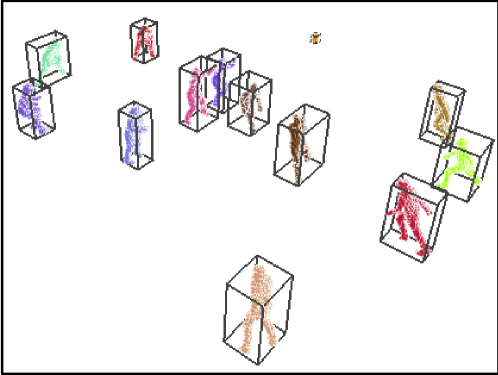
Figure 4: 3D ROI extraction for sparse point cloud.

\begin{overpic}[width=433.62pt]{isovalue-eps-converted-to.pdf} \end{overpic}

(a)

\begin{overpic}[width=433.62pt]{intersection-eps-converted-to.pdf} \end{overpic}

(b)

Figure 5: Exact isovalue computation. (a) Project the edges of a grid cell onto image plane. (b) Find the exact intersection using Bresenham’s line algorithm.

II-D Visibility Detection

To determine the visibility of a specific camera $i$, we perform two operations including the computation of the depth image and determination of occlusion.

II-D1 Computation of depth image

We project each triangle on an object surface onto the image plane of camera $i$ to form a 2D triangle. The depth ${}^{i}D^{j}_{m}$ of a pixel $j$ that is bounded by the $m-$th 2D triangle is assigned the distance from its corresponding 3D triangle to the camera center. After projecting all the triangles, the depth ${}^{i}D^{j}$ of a pixel $j$ is determined by Eq. (4).

$${}^{i}D^{j}=\min\left\{{}^{i}D^{j}_{1},{}^{i}D^{j}_{2},\cdots,{}^{i}D^{j}_{M}\right\}{.}$$ (4)

Here, $M$ expresses the number of 3D triangles corresponding with pixel $j$. The upper image in Fig. 1 (d) shows the computed depth image, in which the darker color indicates that the distance to the camera center is greater. To find the pixels bounded by a triangle, we assume that a triangle is orientable and the bounded pixel is on the same side of each edge.

II-D2 Visibility detection

The visibility of each triangle in each camera is tested by comparing the distance from the triangle to a camera plane with the cached value in the depth image. If the difference is larger than a threshold $T_{v}$, we consider that the triangle is occluded. The bottom image in Fig. 1 (d) presents an occlusion map of a specific camera where the occluded parts are shown in grey. It should be noted that $T_{v}$ is assigned a high value in our implementation so that the self-occlusion is ignored.

II-E View-dependent Rendering

When users experience FVV, the 3D coordinate and the direction of a virtual viewpoint are calculated. The uppermost reference camera for rendering is identified as the nearest camera by calculating the distance from the virtual viewpoint to each camera. Coupled with the occlusion maps, the non-occluded parts are rendered by the uppermost reference camera, while the neighboring cameras render the occluded regions.

\begin{overpic}[width=433.62pt]{camera-position-eps-converted-to.pdf} \end{overpic}

(a) Camera configuration

\begin{overpic}[width=433.62pt]{record-screen-eps-converted-to.pdf} \end{overpic}

(b) Recording environment

Figure 6: System overview.

\begin{overpic}[width=433.62pt]{1st-cam01-eps-converted-to.pdf} \end{overpic}

(a) The first content

\begin{overpic}[width=433.62pt]{2nd-cam01-eps-converted-to.pdf} \end{overpic}

(b) The second content

Figure 7: The input image of the Volleyball contents.

III EXPERIMENTS

\begin{overpic}[width=433.62pt]{billboard-experimental-results-eps-converted-to.pdf} \end{overpic}

(a)

\begin{overpic}[width=433.62pt]{conventional-experimental-results-eps-converted-to.pdf} \end{overpic}

(b)

\begin{overpic}[width=433.62pt]{proposed-experimental-results-eps-converted-to.pdf} \end{overpic}

(c)

Figure 8: Synthesized FVV of the first volleyball sequence viewing from a virtual viewpoint. (a) result by [6]. (b) result by [20]. (c) result by our method. The left bottom figure of (a) is reconstructed binary 2D billboard while the left bottom figure of (b) and (c) are reconstructed 3D polygonal mesh.

\begin{overpic}[width=433.62pt]{billboard-experimental-results-2-eps-converted-to.pdf} \end{overpic}

(a)

\begin{overpic}[width=433.62pt]{conventional-experimental-results-2-eps-converted-to.pdf} \end{overpic}

(b)

\begin{overpic}[width=433.62pt]{proposed-experimental-results-2-eps-converted-to.pdf} \end{overpic}

(c)

Figure 9: Synthesized FVV of the second volleyball sequence viewing from a virtual viewpoint. (a) result by [6]. (b) result by [20]. (c) result by our method. The left bottom figure of (a) is reconstructed binary 2D billboard while the left bottom figure of (b) and (c) are reconstructed 3D polygonal mesh.

\begin{overpic}[width=433.62pt]{judo-real-eps-converted-to.pdf} \end{overpic}

(a) Images captured at different time by a selected camera

\begin{overpic}[width=433.62pt]{judo-billboard-eps-converted-to.pdf} \end{overpic}

(b) Synthesised images by [6]

\begin{overpic}[width=433.62pt]{judo-conventional-eps-converted-to.pdf} \end{overpic}

(c) Synthesised images by [20]

\begin{overpic}[width=433.62pt]{judo-proposed-eps-converted-to.pdf} \end{overpic}

(d) Synthesised images by the proposed method

Figure 10: Synthesized FVV of a judo sequence with a virtual stadium model

III-A Visual quality evaluation

To demonstrate the performance of our method, we compared it to two approaches. The first one [6] is a billboard-based method that reconstructs a billboard for each object including an occluded object by employing a rough 3D model. The second one [20] is a typical 3D model-based method that approximates the object shape using visual hull and builds the mesh representation using the conventional marching cubes algorithm.

We initially evaluated the proposed method with volleyball sequences that are captured with ten synchronized cameras. The resolution of each camera was $3840\times 2160$, and the frame rate is $30~{}$fps. The target space for reconstruction was set to $18~{}$meters wide, $18~{}$meters deep, and $9~{}$meters high. Fig. 6 shows the camera configuration in the stadium and recording environment. The camera threshold in [6] for the reconstruction of a rough 3D shape is $9$, while the isovalue for isosurface extraction in [20] is $0.5$. The voxel size in all the three methods is $2\,cm$ $\times$ $2\,cm$ $\times$ $2\,cm$. Fig. 7 shows the input images of two volleyball contents captured by camera $01$. It can be seen that the players in the red rectangular are occluded. Fig. 8 and 9 demonstrate virtual viewpoint images generated by the three methods. The top row shows the synthesized representations of the whole scene, while the bottom row presents reconstructed models (2D billboard or 3D polygon mesh) and close-up views. The virtual viewpoint images are rendered mainly by camera $01$ because it is the camera nearest to the virtual viewpoint. First, let us focus on the results by [6] (shown in Fig. 8 (a) and 9 (a)). The binary 2D billboard on the left bottom illustrates that this method can estimate the pose of an object reasonably, while the close-up view on the right bottom shows that some occluded regions failed to be rendered. Next, let us look at the results by [20] (shown in Fig. 8 (b) and 9 (b)). We found that [20] produces jagged artifacts in the surface of the reconstructed polygonal mesh, which affect the quality of rendering. From the close-up view, it can be seen that black noise exists in the object boundary. Furthermore, the appearance of the occluded area is misaligned. As for the results by our approach (shown in Fig. 8 (c) and 9 (c)), it can be observed that the reconstructed polygonal mesh is smooth, while the color appearance of occluded regions was appropriately reproduced.

A judo sequence that is captured with sixteen synchronized cameras was also employed to evaluate the visual quality of virtual images synthesized using the proposed method. The resolution of captured images is $1920\times 1080$ while the predefined 3D volume is $5\,m$ $\times$ $6\,m$ $\times$ $2.1\,m$. For all the methods, voxel size for 3D reconstruction is kept at $4\,cm$ $\times$ $4\,cm$ $\times$ $4\,cm$. The camera threshold in [6] and the isovalue in [20] are $14$ and $0.5$, respectively. Fig. 10 (a) presents the input images of a selected camera, which were captured at different times. Fig. 10 (b), (c), and (d) show the synthesized images obtained by the three methods with a virtual stadium model. The red rectangular on the virtual playground is a point of reference, allowing people to sense the difference among the synthesized images. Concerning the results in (b), it can be seen that the position and shape of reconstructed objects are different from those obtained by 3D modeling methods even though their virtual viewpoints are the same. The reason for this phenomenon is that the objects in (b) are represented by 2D billboards that cannot describe the exact 3D pose of each object. Regarding the results in (c), the boundary of the reconstructed objects is jagged. The imprecise polygonization in [20] decreases the realistic visual effect. The observation from (c) is that the reconstructed model retains the same pose with those obtained by [20] while the object boundary is smooth and natural.

III-B Execution time evaluation

In the production of FVV, steps (B)–(D) are accelerated by executing them in parallel on a GPU board on the server side, while step (E), rendering, runs on the client side. To achieve high computational efficiency, we grab all the memory the production needs from GPU immediately at startup of the application. The data transfer between CPU and GPU and processes for production are managed separately by two CPU threads. The reference methods, [6] and [20], are implemented in the same manner. We use a PC with Intel(R) Core(TM) i7-6700K CPU, 4.00 GHz $\And$ 4.00 GHz, 32.0 GB RAM, NVIDIA Geforce GTX 1080Ti and Windows 7 Professional Service Pack 1.

TABLE I: Execution time of production in milliseconds.

	[6]	[20]	proposed
1st Volleyball content	15650.15	1411.59	36.39
2nd Volleyball content	14006.47	1436.17	33.66
Judo content	956.58	17.73	7.30

Table I shows the execution time for the processes in CUDA excluding the time taken for device memory allocation and data transfer when the voxel sizes for sparse and dense volumetric visual hull approximation for the three sets of content are respectively $\left(50\,mm,20\,mm\right)$, $\left(50\,mm,20\,mm\right)$ and $\left(80\,mm,40\,mm\right)$. The reported execution time is the average over $200$ continuous frames to remove any fluctuations caused by the different distributions of the athletes. The creation of 2D billboards swamped the computation time of [6]. It created 130 and 32 billboards for the volleyball and judo sequences, respectively. As for [20], the noise filtering is the most time-consuming component that contributes to the production and accounted for around $90\%$ and $50\%$ for the volleyball and judo sequences, respectively. The different percentages indicate that the execution time changes significantly as the resolution of the pre-defined volume increases. Comparing these results, the proposed method can be executed more quickly than the other methods. Moreover, it demonstrated consistent performances for the three sequences. The average execution times for each of the production processes are shown in Table II. These times indicate that the noise filtering and ROI extraction still consume the most time, especially for a sports event taking place in a large space.

TABLE II: Execution time for each process in milliseconds.

	1st V	2nd V	Judo
(B-1) Sparse visual hull	0.54	0.58	0.06
(B-2) Noise filtering & 3D ROI extraction	21.49	19.75	2.11
(B-3) Dense visual hull	1.23	1.13	0.23
(C) Polygonization	3.90	3.67	0.65
(D-1) Computation of depth image	5.93	5.52	2.99
(D-2) Visibility detection	3.30	3.01	1.26

III-C Discussion of parameters

To clarify the effect of voxel sizes on execution time, we performed another two experiments with the first volleyball sequence. In the first experiments, we conducted FVV production while varying the voxel size for sparse visual hull from $20~{}$mm to $60~{}$mm (stride is $10~{}$mm) but keeping the voxel size for dense visual hull steady at $20~{}$mm. Fig. 11 (a) shows the execution times. When the voxel size for both coarse and fine visual hull construction is $20~{}$mm, the acceleration function is disabled. The time consumed in this case is around $310~{}$ms, which was the highest among the tests. The time curve proves that the execution time has a positive association with the voxel size for sparse visual hull. It can be reduced by increasing the voxel size. Fig. 11 (b) presents the time consumed in the second experiments, in which we varied the voxel size for dense visual hull from $15~{}$mm to $35~{}$mm (stride is $5~{}$mm) but kept the voxel size for sparse visual hull steady at $50~{}$mm. The results indicate that the number of voxels in dense visual hull construction does not have a marked effect on production time.

\begin{overpic}[width=433.62pt]{exe-time-sparse-eps-converted-to.pdf} \end{overpic}

(a) different voxel sizes for sparse visual hull

\begin{overpic}[width=433.62pt]{exe-time-dense-eps-converted-to.pdf} \end{overpic}

(b) different voxel sizes for dense visual hull

Figure 11: Execution time versus different voxel sizes.

IV CONCLUSIONS

In this paper, we proposed a novel parallel approach to solve the fast FVV synthesis issue that occurs in sports scenario. Our method first employs a sparse-to-fine volumetric visual hull construction strategy to reduce the time needed for 3D shape approximation and then applies an accurate isosurface extraction method to give a high-quality mesh representation to the 3D model. Coupled with the occlusion map in each camera, the appearance of the scene at a virtual viewpoint is reproduced in a view-dependent manner. We implemented the proposed method on a PC with a GPU and verified its performance with volleyball and judo sequences. The experimental results show that our method outperforms existing approaches in terms of both visual quality and execution time.

References

- [1] Takeo Kanade, Peter Rander, and PJ Narayanan, “Virtualized reality: Constructing virtual worlds from real scenes,” IEEE multimedia, vol. 4, no. 1, pp. 34–47, 1997.
- [2] Takashi Matsuyama and Takeshi Takai, “Generation, visualization, and editing of 3d video,” in null. IEEE, 2002, p. 234.
- [3] Jean-Yves Guillemaut and Adrian Hilton, “Joint multi-layer segmentation and reconstruction for free-viewpoint video applications,” International journal of computer vision, vol. 93, no. 1, pp. 73–100, 2011.
- [4] Marcel Germann, Tiberiu Popa, Richard Keiser, Remo Ziegler, and Markus Gross, “Novel-view synthesis of outdoor sport events using an adaptive view-dependent geometry,” in Computer Graphics Forum. Wiley Online Library, 2012, vol. 31, pp. 325–333.
- [5] Keisuke Nonaka, Ryosuke Watanabe, Jun Chen, Houari Sabirin, and Sei Naito, “Fast plane-based free-viewpoint synthesis for real-time live streaming,” in IEEE International Conference on Visual Communications and Image Processing. IEEE, 2018.
- [6] Hiroshi Sankoh, Sei Naito, Keisuke Nonaka, Houari Sabirin, and Jun Chen, “Robust billboard-based, free-viewpoint video synthesis algorithm to overcome occlusions under challenging outdoor sport scenes,” in Proceedings of the 26th ACM International Conference on Multimedia. 2018, MM ’18, pp. 1724–1732, ACM.
- [7] Kunihiko Hayashi and Hideo Saito, “Synthesizing free-viewpoing images from multiple view videos in soccer stadiumadium,” in Computer Graphics, Imaging and Visualisation, 2006 International Conference on. IEEE, 2006, pp. 220–225.
- [8] Keisuke Nonaka, Qiang Yao, Houari Sabirin, Jun Chen, Hiroshi Sankoh, and Sei Naito, “Billboard deformation via 3d voxel by using optimization for free-viewpoint system,” in 2017 25th European Signal Processing Conference (EUSIPCO). IEEE, 2017, pp. 1500–1504.
- [9] Keisuke Nonaka, Houari Sabirin, Jun Chen, Hiroshi Sankoh, and Sei Naito, “Optimal billboard deformation via 3d voxel for free-viewpoint system,” IEICE TRANSACTIONS on Information and Systems, vol. 101, no. 9, pp. 2381–2391, 2018.
- [10] Houari Sabirin, Qiang Yao, Keisuke Nonaka, Hiroshi Sankoh, and Sei Naito, “Toward real-time delivery of immersive sports content,” IEEE MultiMedia, vol. 25, no. 2, pp. 61–70, 2018.
- [11] Joe Kilner, Jonathan Starck, Adrian Hilton, and Oliver Grau, “Dual-mode deformable models for free-viewpoint video of sports events,” in Sixth International Conference on 3-D Digital Imaging and Modeling (3DIM 2007). IEEE, 2007, pp. 177–184.
- [12] Yebin Liu, Qionghai Dai, and Wenli Xu, “A point-cloud-based multiview stereo algorithm for free-viewpoint video,” IEEE transactions on visualization and computer graphics, vol. 16, no. 3, pp. 407–418, 2010.
- [13] Greg Slabaugh, Ron Schafer, Tom Malzbender, and Bruce Culbertson, “A survey of methods for volumetric scene reconstruction from photographs,” in Volume Graphics 2001. Springer, 2001, pp. 81–100.
- [14] Steven M Seitz and Charles R Dyer, “Photorealistic scene reconstruction by voxel coloring,” International Journal of Computer Vision, vol. 35, no. 2, pp. 151–173, 1999.
- [15] Carlos Hernández Esteban and Francis Schmitt, “Silhouette and stereo fusion for 3d object modeling,” Computer Vision and Image Understanding, vol. 96, no. 3, pp. 367–392, 2004.
- [16] Sudipta N Sinha and Marc Pollefeys, “Multi-view reconstruction using photo-consistency and exact silhouette constraints: A maximum-flow formulation,” in Computer Vision, 2005. ICCV 2005. Tenth IEEE International Conference on. IEEE, 2005, vol. 1, pp. 349–356.
- [17] Jonathan Starck and Adrian Hilton, “Surface capture for performance-based animation,” IEEE computer graphics and applications, vol. 27, no. 3, 2007.
- [18] Konstantinos Rematas, Ira Kemelmacher-Shlizerman, Brian Curless, and Steve Seitz, “Soccer on your tabletop,” in Proceedings of the IEEE Conference on Computer Vision and Pattern Recognition, 2018, pp. 4738–4747.
- [19] German KM Cheung, Takeo Kanade, J-Y Bouguet, and Mark Holler, “A real time system for robust 3d voxel reconstruction of human motions,” in Computer Vision and Pattern Recognition, 2000. Proceedings. IEEE Conference on. IEEE, 2000, vol. 2, pp. 714–720.
- [20] Aljoscha Smolic, “3d video and free viewpoint video—from capture to display,” Pattern recognition, vol. 44, no. 9, pp. 1958–1968, 2011.
- [21] J-Y Bouguet, “Camera calibration toolbox for matlab,” http://www. vision. caltech. edu/bouguetj/calib_doc/index. html, 2004.
- [22] Kaiming He, Georgia Gkioxari, Piotr Dollár, and Ross Girshick, “Mask r-cnn,” in Computer Vision (ICCV), 2017 IEEE International Conference on. IEEE, 2017, pp. 2980–2988.
- [23] Morita Shinji, Yamazawa Kazumasa, and Terasawa Seihiko, “Networked remote survemilnce system using omnidirectionalimage sensors,” Transactions of the IEICE D, vol. 88, no. 5, pp. 864–875, 2005.
- [24] Jun Chen, Keisuke Nonaka, Hiroshi Sankoh, Ryosuke Watanabe, Houari Sabirin, and Sei Naito, “Efficient parallel connected component labeling with a coarse-to-fine strategy,” IEEE Access, vol. 6, pp. 55731–55740, 2018.