Replica symmetry breaking in random matrix model: a toy model of wormhole networks

Abstract

We study the replica symmetry breaking (RSB) in the Gaussian Unitary Ensemble (GUE) random matrix model. We find that the RSB occurs at the transition temperature $T_{\text{RSB}}\sim N^{-2/3}$ in the large $N$ limit. We argue that this transition originates from a landscape of almost degenerate local minima of free energy labeled by Young diagrams. We also discuss a possible implication of our findings for the multiply-coupled Sachdev-Ye-Kitaev models and their holographic dual Jackiw-Teitelboim gravity from the viewpoint of ER=EPR conjecture.

1 Introduction

The replica symmetry breaking (RSB) in disordered system is an important concept in the study of glass transition. In particular, the spin-glass model of Sherrington and Kirkpatrick SKmodel was solved by Parisi parisi1 ; parisi2 based on the RSB ansatz (see Denef:2011ee for a review).

In the disordered system a natural quantity to compute is the quenched average of the free energy $\langle\log Z(\beta)\rangle$, where $Z(\beta)=\operatorname{Tr}e^{-\beta H}$ is the partition function and $\beta$ is the inverse of temperature $T$

$$\beta=\frac{1}{T}.$$ (1)

The average $\langle\cdots\rangle$ in the disordered system is defined by integrating over the distribution of random couplings in the Hamiltonian $H$. The replica method is commonly used to compute the quenched average $\langle\log Z(\beta)\rangle$ by preparing $n$ copies of the system (replicas) and taking the limit $n\to 0$ at the end of calculation

$$\langle\log Z(\beta)\rangle=\lim_{n\to 0}\frac{\partial}{\partial n}\langle Z(\beta)^{n}\rangle.$$ (2)

RSB is characterized by the condition that the quenched average and the annealed average of $n$ replicas do not agree

$$\langle Z(\beta)^{n}\rangle\neq\langle Z(\beta)\rangle^{n}.$$ (3)

In this paper, we consider the RSB in the Gaussian Unitary Ensemble (GUE) random matrix model, where the random couplings in the Hamiltonian are modeled by treating the Hamiltonian $H$ itself as a random $N\times N$ hermitian matrix with the Gaussian distribution

$$\langle\cdots\rangle=\frac{\int dHe^{-\frac{N}{2}\operatorname{Tr}H^{2}}(\cdots)}{\int dHe^{-\frac{N}{2}\operatorname{Tr}H^{2}}}.$$ (4)

Note that the RSB in the GUE random matrix model has been considered in kamenev , where the correlator of resolvent $\operatorname{Tr}(E-H)^{-1}$ was studied by the replica method. In this paper we consider the correlator of $Z(\beta)=\operatorname{Tr}e^{-\beta H}$ and study the RSB characterized by (3). We will not consider the limit $n\to 0$ in (2); we study $\langle Z(\beta)^{n}\rangle$ with positive integer $n$ in its own right.

We find that in the large $N$ limit $\langle Z(\beta)^{n}\rangle$ in the GUE random matrix model indeed exhibits the RSB at the transition temperature $T_{\text{RSB}}$

$$\langle Z(\beta)^{n}\rangle\approx\left\{\begin{aligned} &\langle Z(\beta)\rangle^{n},&\quad&(T>T_{\text{RSB}}),\\ &\langle Z(\beta)^{n}\rangle_{c},&\quad&(T<T_{\text{RSB}}),\end{aligned}\right.$$ (5)

where the subscript $c$ in $\langle Z(\beta)^{n}\rangle_{c}$ denotes the connected part of the correlator. A similar behavior was observed in the so-called random-energy model, where each energy levels are assumed to be Gaussian distributed but the correlations between different energy levels are neglected Derrida . It turns out that $T_{\text{RSB}}$ for the GUE matrix model scales as

$$T_{\text{RSB}}\sim N^{-2/3}.$$ (6)

We will argue that the transition at $T=T_{\text{RSB}}$ originates from the existence of a landscape of almost degenerate local minima of free energy. This landscape of local minima arises as follows: When we expand $\langle Z(\beta)^{n}\rangle$ in terms of the connected correlators, there appear many terms labeled by Young diagrams. Each term of this expansion can be thought of as a local minimum of free energy.

We will also discuss a possible implication of our findings for the Sachdev-Ye-Kitaev (SYK) model kitaev ; Maldacena:2016hyu and its holographic dual Jackiw-Teitelboim (JT) gravity Jackiw:1984je ; Teitelboim:1983ux ; Almheiri:2014cka . We examine the idea that the connected part of correlator $\langle Z(\beta)^{n}\rangle_{c}$ corresponds to a dual spacetime geometry where the $n$ boundaries are connected by an $n$-pronged Euclidean wormhole. We speculate that around the RSB transition temperature the dual gravity side does not corresponds to a classical geometry, but a superposition of random wormhole networks.

This paper is organized as follows. In section 2, we first review the exact result of $\langle Z(\beta)^{n}\rangle$ at finite $N$ in the GUE random matrix model. In section 3, we study the RSB of $\langle Z(\beta)^{n}\rangle$ in the GUE random matrix model using the exact result at finite $N$. In section 4, we discuss possible implications of our findings in the GUE matrix model for the multiply-coupled SYK models and their dual JT gravity.

2 Review of the exact results of GUE random matrix model

In this section, we review the known results of the correlation function $\langle Z(\beta)^{n}\rangle$ in the GUE random matrix model (4). As pointed out in delCampo:2017bzr ; Okuyama:2018yep , this quantity is formally equivalent to the expectation value of the 1/2 BPS Wilson loops in 4d $\mathcal{N}=4$ $U(N)$ super Yang-Mills (SYM) theory under the identification

$$\sqrt{\lambda}\leftrightarrow 2\beta,$$ (7)

where $\lambda$ is the ’t Hooft coupling of $\mathcal{N}=4$ SYM. Thus we can immediately find the exact finite $N$ expression of $\langle Z(\beta)^{n}\rangle$ by borrowing the known result of $\mathcal{N}=4$ SYM.

We can naturally decompose $\langle Z(\beta)^{n}\rangle$ into the connected components $\langle Z(\beta)^{j}\rangle_{c}~{}(j=1,\cdots,n)$. The relation between $\langle Z(\beta)^{n}\rangle$ and the connected part $\langle Z(\beta)^{j}\rangle_{c}$ is compactly expressed in terms of the generating function, as usual

$$\bigl{\langle}e^{\alpha Z(\beta)}\bigr{\rangle}=\sum_{n=0}^{\infty}\frac{\alpha^{n}}{n!}\langle Z(\beta)^{n}\rangle=\exp\Biggl{[}\sum_{j=1}^{\infty}\frac{\alpha^{j}}{j!}\langle Z(\beta)^{j}\rangle_{c}\Biggr{]},$$ (8)

where $\alpha$ is a formal expansion parameter. For instance, $\langle Z(\beta)^{n}\rangle$ with $n=2,3,4$ are expanded as

$$\langle Z(\beta)^{2}\rangle =\langle Z(\beta)\rangle^{2}+\langle Z(\beta)^{2}\rangle_{c},$$ (9)

$$\langle Z(\beta)^{3}\rangle =\langle Z(\beta)\rangle^{3}+3\langle Z(\beta)\rangle\langle Z(\beta)^{2}\rangle_{c}+\langle Z(\beta)^{3}\rangle_{c},$$

$$\langle Z(\beta)^{4}\rangle =\langle Z(\beta)\rangle^{4}+6\langle Z(\beta)\rangle^{2}\langle Z(\beta)^{2}\rangle_{c}+3\langle Z(\beta)^{2}\rangle_{c}^{2}+4\langle Z(\beta)\rangle\langle Z(\beta)^{3}\rangle_{c}+\langle Z(\beta)^{4}\rangle_{c}.$$

In general, the expansion of $\langle Z(\beta)^{n}\rangle$ is characterized by the partition of $n$ labeled by a Young diagram $Y$

$$Y=[1^{k_{1}}2^{k_{2}}\cdots n^{k_{n}}],\qquad|Y|=\sum_{j=1}^{n}jk_{j}=n,$$ (10)

and (9) for general $n$ becomes

$$\langle Z(\beta)^{n}\rangle=\sum_{|Y|=n}\mathcal{Z}_{Y}(\beta),$$ (11)

where $\mathcal{Z}_{Y}(\beta)$ is given by

$$\mathcal{Z}_{Y}(\beta)=n!\prod_{j=1}^{n}\frac{1}{k_{j}!}\left[\frac{\langle Z(\beta)^{j}\rangle_{c}}{j!}\right]^{k_{j}}.$$ (12)

For example, $[1^{n}]$ and $[n]$ correspond to the totally disconnected and the totally connected part, respectively

$$\mathcal{Z}_{[1^{n}]}(\beta)=\langle Z(\beta)\rangle^{n},\qquad\mathcal{Z}_{[n]}(\beta)=\langle Z(\beta)^{n}\rangle_{c}.$$ (13)

As shown in Okuyama:2018aij , we can write down the exact finite $N$ result of $\langle Z(\beta)^{n}\rangle_{c}$ in terms of the $N\times N$ matrix $A(\beta)$

$$A(\beta)_{i,j}=e^{\frac{\beta^{2}}{2N}}\sqrt{\frac{i!}{j!}}\left(\frac{\beta}{\sqrt{N}}\right)^{j-i}L_{i}^{j-i}\left(-\frac{\beta^{2}}{N}\right),\qquad(i,j=0,\cdots,N-1),$$ (14)

where $L_{n}^{\alpha}(x)$ denotes the associated Laguerre polynomial. The one-point function $\langle Z(\beta)\rangle$ is simply given by the trace of $A(\beta)$

$$\langle Z(\beta)\rangle=\operatorname{Tr}A(\beta)=e^{\frac{\beta^{2}}{2N}}L_{N-1}^{1}\left(-\frac{\beta^{2}}{N}\right).$$ (15)

Similarly, the connected part $\langle Z(\beta)^{n}\rangle_{c}$ is given by some combination of $A(\beta)$ Okuyama:2018aij

$$\langle Z(\beta)^{n}\rangle_{c}=\oint\prod_{i=1}^{n}\frac{dz_{i}}{2\pi\mathrm{i}z_{i}^{2}}\operatorname{Tr}\log\left[\sum_{m=0}^{n}\sum_{i_{1}<\cdots<i_{m}}z_{i_{1}}\cdots z_{i_{m}}A(m\beta)\right].$$ (16)

For instance, $\langle Z(\beta)^{2}\rangle_{c}$ is given by

$$\langle Z(\beta)^{2}\rangle_{c} =\oint\frac{dz_{1}}{2\pi\mathrm{i}z_{1}^{2}}\oint\frac{dz_{2}}{2\pi\mathrm{i}z_{2}^{2}}\operatorname{Tr}\log\Bigl{[}1+z_{1}A(\beta)+z_{2}A(\beta)+z_{1}z_{2}A(2\beta)\Bigr{]}$$ (17)

$$=\operatorname{Tr}\Bigl{[}A(2\beta)-A(\beta)^{2}\Bigr{]}.$$

In a similar manner, one can write down $\langle Z(\beta)^{3}\rangle_{c}$ and $\langle Z(\beta)^{4}\rangle_{c}$ as

$$\langle Z(\beta)^{3}\rangle_{c} =\operatorname{Tr}\Bigl{[}A(3\beta)-3A(\beta)A(2\beta)+2A(\beta)^{3}\Bigr{]},$$ (18)

$$\langle Z(\beta)^{4}\rangle_{c} =\operatorname{Tr}\Bigl{[}A(4\beta)-4A(\beta)A(3\beta)-3A(2\beta)^{2}+12A(\beta)^{2}A(2\beta)-6A(\beta)^{4}\Bigr{]}.$$

Using these exact results (17) and (18), in the next section we will numerically study the behavior of $\langle Z(\beta)^{n}\rangle~{}(n=2,3,4)$ in (9).

Next, let us briefly summarize the known results of $\langle Z(\beta)^{n}\rangle$ in the large $N$ limit. In the large $N$ limit, the eigenvalues of $H$ with the Gaussian measure (4) are distributed along the cut $[E_{0},-E_{0}]$ with the eigenvalue density $\rho(E)$ obeying the Wigner semi-circle law

$$\rho(E)=\frac{2}{\pi E_{0}^{2}}\sqrt{E_{0}^{2}-E^{2}}.$$ (19)

In our normalization of the measure (4), the “ground state energy” $E_{0}$ is given by

$$E_{0}=-2.$$ (20)

The eigenvalue density (19) is a property of a single eigenvalue. One can consider the correlation of $n$ eigenvalues characterized by the correlation function $\rho^{(n)}(E_{1},\cdots,E_{n})$. It turns out that $\rho^{(n)}$ is written in terms of the kernel $K$ (see e.g. Mehta )

$$K(E,E^{\prime})=\sum_{\ell=0}^{N-1}\psi_{\ell}(E)\psi_{\ell}(E^{\prime}),$$ (21)

where $\psi_{\ell}(E)$ is the wavefunction associated with the measure (4), i.e. the wavefunction of harmonic oscillator in this case

$$\psi_{\ell}(E)=\left(\frac{N}{2\pi}\right)^{\frac{1}{4}}\frac{1}{\sqrt{2^{\ell}\ell!}}H_{\ell}\left(\sqrt{\frac{N}{2}}E\right)e^{-\frac{NE^{2}}{4}}.$$ (22)

Here $H_{\ell}(x)$ denotes the Hermite polynomial of order $\ell$. Note that the eigenvalue density is given by the diagonal part of the kernel $K$

$$\rho(E)=\frac{1}{N}K(E,E).$$ (23)

Now $\langle Z(\beta)^{n}\rangle$ is written in terms of $K$ as

$$\langle Z(\beta)^{n}\rangle =\int\prod_{i=1}^{n}dE_{i}e^{-\beta E_{i}}\det\Bigl{[}K(E_{k},E_{l})\Bigr{]}_{k,l=1,\cdots,n}$$ (24)

$$=\sum_{\sigma\in S_{n}}(-1)^{\sigma}\int\prod_{i=1}^{n}dE_{i}e^{-\beta E_{i}}K(E_{i},E_{\sigma(i)}).$$

One can show that the decomposition (11) corresponds to the sum over the conjugacy class of $\sigma\in S_{n}$ in (24). The totally connected part $\mathcal{Z}_{[n]}(\beta)=\langle Z(\beta)^{n}\rangle_{c}$ comes from the cyclic permutation with length $n$

$$\langle Z(\beta)^{n}\rangle_{c}=(-1)^{n-1}\sum_{a=1}^{n-1}\int\prod_{i=1}^{n}dE_{i}e^{-\beta E_{i}}K(E_{i},E_{i+a})$$ (25)

where the subscript of $E_{i}$ is defined modulo $n$ ($E_{i+n}\equiv E_{i}$).

The leading order behavior of $\langle Z(\beta)^{n}\rangle_{c}$ in the large $N$ expansion can be easily found by borrowing the known results of $\mathcal{N}=4$ SYM in Erickson:2000af ; Akemann:2001st ; Giombi:2009ms via the dictionary (7)

$$\langle Z(\beta)\rangle =\frac{N}{\beta}I_{1}(2\beta),$$ (26)

$$\langle Z(\beta)^{2}\rangle_{c} =\beta I_{0}(2\beta)I_{1}(2\beta),$$

$$\langle Z(\beta)^{3}\rangle_{c} =\frac{\beta^{3}}{N}\Bigl{[}I_{0}(2\beta)^{3}+3I_{0}(2\beta)^{2}I_{1}(2\beta)\Bigr{]},$$

where $I_{\nu}(z)$ denotes the modified Bessel function of the first kind. Note that in the large $N$ limit $\langle Z(\beta)^{n}\rangle_{c}$ scales as

$$\langle Z(\beta)^{n}\rangle_{c}\sim N^{\chi},$$ (27)

where $\chi$ is the Euler number of a sphere with $n$ punctures

$$\chi=2-n.$$ (28)

3 RSB in the GUE random matrix model

In this section, we will study the RSB in the GUE random matrix model using the exact result reviewed in the previous section 2.

3.1 Numerical analysis of RSB

To see the RSB in (5), let us consider the ratio between the annealed average $\langle Z(\beta)\rangle^{n}$ and the quenched average $\langle Z(\beta)^{n}\rangle$

$$R_{n}(\beta)=\frac{\langle Z(\beta)\rangle^{n}}{\langle Z(\beta)^{n}\rangle}.$$ (29)

We can numerically study the behavior of $R_{n}(\beta)~{}(n=2,3,4)$ as a function of $\beta$ using the exact result of $\langle Z(\beta)\rangle$ in (15) and $\langle Z(\beta)^{n}\rangle_{c}~{}(n=2,3,4)$ in (17) and (18), together with the relation (9). It turns out that $R_{n}(\beta)$ is conveniently described by the scaling variable $\beta^{\prime}$ defined by

$$\beta^{\prime}=\frac{\beta}{N^{2/3}}.$$ (30)

In Figure 1, we plot $R_{n}(\beta)~{}(n=2,3,4)$ as a function of $\beta^{\prime}$ for $N=60$ (red curves) and $N=100$ (blue dots). As we can see from Figure 1, the plots of $R_{n}(\beta)$ for $N=60$ and $N=100$ are almost identical in the region $\beta^{\prime}\lesssim 2$. This justifies a posteriori our definition of the scaling variable $\beta^{\prime}$ in (30). One can see from Figure 1 that $R_{n}(\beta)$ decays to zero about $\beta^{\prime}\sim 1$. This indicates that the replica symmetry is broken in the low temperature regime $\beta^{\prime}\gtrsim 1$, and the critical value of $\beta$ is roughly given by

$$\beta_{\text{RSB}}\sim N^{2/3},$$ (31)

which corresponds to the temperature $T_{\text{RSB}}$ in (6). In the next subsection, we consider an analytic explanation of the $N$-dependence of the transition temperature in (31).

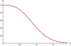
(a) $R_{2}(\beta)$

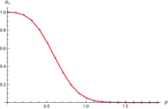
(b) $R_{3}(\beta)$

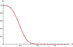
(c) $R_{4}(\beta)$

Figure 1: Plot of $R_{n}(\beta)$ for 1(a) $n=2$, 1(b) $n=3$, and 1(c) $n=4$. Note that the horizontal axis is $\beta^{\prime}=\beta/N^{2/3}$. The red curve is the plot for $N=60$, while the blue dots represent the value of $R_{n}(\beta)$ for $N=100$.

For $n=2$, the decay of $R_{2}(\beta)$ means that in the low temperature region $T<T_{\text{RSB}}$ the connected part $\langle Z(\beta)^{2}\rangle_{c}$ becomes dominant, and around the transition temperature $T\sim T_{\text{RSB}}$ it takes place the exchange of dominance between the connected part $\langle Z(\beta)^{2}\rangle_{c}$ and the disconnected part $\langle Z(\beta)\rangle^{2}$. However, for $n\geq 3$ what is happening around $T\sim T_{\text{RSB}}$ is more involved since $\langle Z(\beta)^{n}\rangle$ has many terms (11) when written in terms of the combination of connected correlators. We will study the detailed structure for $n\geq 3$ in section 3.3.

3.2 Analytic estimate of the transition temperature

In this subsection, we will estimate the transition temperature using the large $N$ result of $\langle Z(\beta)^{n}\rangle_{c}$ in (26). From the asymptotic behavior of the modified Bessel function

$$I_{\nu}(z)\sim\frac{e^{z}}{\sqrt{2\pi z}},\qquad(z\gg 1),$$ (32)

one can see that in the regime $\beta\gg 1$, $\langle Z(\beta)^{n}\rangle_{c}$ in (26) behaves as

$$\langle Z(\beta)^{n}\rangle_{c}\sim\left(\frac{N}{\beta^{3/2}}\right)^{2-n}e^{2n\beta}.$$ (33)

As discussed in Drukker:2000rr , the combination $\beta^{3/2}/N$ appearing in (33) has a natural interpretation as the effective genus counting parameter

$$g_{\text{eff}}=\frac{\beta^{3/2}}{N}.$$ (34)

Indeed, the large $N$ expansion of the exact finite $N$ result (15), (17) and (18) beyond the leading order (26) are organized as the genus expansion with the effective string coupling in (34) Drukker:2000rr . In terms of this effective string coupling $g_{\text{eff}}$, (33) is written as

$$\langle Z(\beta)^{n}\rangle_{c}\sim g_{\text{eff}}^{-\chi}e^{-n\beta E_{0}}$$ (35)

where $\chi$ is defined in (28) and $E_{0}=-2$ (20). (35) should be compared with the disconnected part

$$\langle Z(\beta)\rangle^{n}\sim\Bigl{(}g_{\text{eff}}^{-1}e^{-\beta E_{0}}\Bigr{)}^{n}=g_{\text{eff}}^{-n}e^{-n\beta E_{0}}.$$ (36)

The connected part (35) and the disconnected part (36) become comparable when the effective string coupling becomes of order $1$

$$g_{\text{eff}}\sim 1.$$ (37)

From (34), this condition explains the $N$-dependence of the transition temperature $\beta_{\text{RSB}}$ in (31).

The scaling (33) for $n=1$ is easily understood from the behavior of the eigenvalue density near the ground state $E\sim E_{0}$. In the low temperature regime $\beta\gg 1$ the dominant contribution to the integral

$$\langle Z(\beta)\rangle=N\int_{E_{0}}^{-E_{0}}dE\rho(E)e^{-\beta E}$$ (38)

comes from the edge of the spectrum near the ground state $E=E_{0}$. Introducing the excitation energy $\mathcal{E}$ from the ground state,

$$\mathcal{E}=E-E_{0},$$ (39)

the eigenvalue density (19) near the ground state $\mathcal{E}\approx 0$ behaves as

$$\rho(E)\sim\sqrt{\mathcal{E}}.$$ (40)

Then (38) is approximated as

$$\langle Z(\beta)\rangle\approx Ne^{-\beta E_{0}}\int d\mathcal{E}\sqrt{\mathcal{E}}e^{-\beta\mathcal{E}}\approx\frac{N}{\beta^{3/2}}e^{-\beta E_{0}},$$ (41)

which reproduces the scaling behavior in (33) for $n=1$. For $n\geq 2$, we could not find a simple scaling argument to derive (33) from the integral representation of $\langle Z(\beta)^{n}\rangle_{c}$ in (25). It would be interesting to understand the behavior (33) directly from (25).

3.2.1 Comparison with the spectral form factor

The spectral form factor (SFF), defined by $\langle Z(\mathrm{i}t)Z(-\mathrm{i}t)\rangle$, is widely studied as a useful diagnostic of quantum chaos jost . In SFF, the exchange of dominance between the connected and the disconnected parts also occurs at the so-called dip time $t_{\text{dip}}$, which can be estimated as follows Cotler:2016fpe . The disconnected part of SFF behaves as

$$\langle Z(\mathrm{i}t)\rangle\langle Z(-\mathrm{i}t)\rangle\sim\left(\frac{N}{t^{3/2}}\right)^{2},$$ (42)

which describes the early time decay of SFF, the so-called “slope.” The origin of the factor $1/t^{3/2}$ in (42) is essentially the same as the calculation in (41). On the other hand, the connected part grows linearly in time, which is known as the “ramp”:

$$\langle Z(\mathrm{i}t)Z(-\mathrm{i}t)\rangle_{c}\sim t.$$ (43)

Equating (42) and (43) we find the time scale of “dip”

$$t_{\text{dip}}\sim N^{1/2}.$$ (44)

The $N$-dependence of $t_{\text{dip}}$ is different from that of the transition temperature $\beta_{\text{RSB}}$ in (31). This is not a contradiction since $\langle Z(\beta)^{2}\rangle$ and the SFF are sensitive to the different aspects of the two-point correlation $\rho^{(2)}(E_{1},E_{2})$ of energy eigenvalues:

$$\langle Z(\beta)^{2}\rangle =\int dE_{1}dE_{2}\,e^{-\beta(E_{1}+E_{2})}\det\Bigl{[}K(E_{i},E_{j})\Bigr{]}_{i,j=1,2},$$ (45)

$$\langle Z(\mathrm{i}t)Z(-\mathrm{i}t)\rangle =\int dE_{1}dE_{2}\,e^{\mathrm{i}t(E_{1}-E_{2})}\det\Bigl{[}K(E_{i},E_{j})\Bigr{]}_{i,j=1,2}.$$

Namely, $\langle Z(\beta)^{2}\rangle$ is the Laplace transform of $\rho^{(2)}$ with respect to the total energy, while SFF is the Fourier transform of $\rho^{(2)}$ with respect to the energy difference.

3.3 Landscape of free energy

The behavior of $\langle Z(\beta)^{n}\rangle_{c}$ in (33) can be easily generalized to arbitrary term $\mathcal{Z}_{Y}(\beta)$ in the expansion (11)

$$\mathcal{Z}_{Y}(\beta)\sim e^{-n\beta E_{0}}\prod_{j=1}^{n}g_{\text{eff}}^{(j-2)k_{j}}.$$ (46)

When $g_{\text{eff}}\sim 1$, not only the totally connected and disconnected terms with $Y=[n]$ and $Y=[1^{n}]$, but all terms in the expansion (11) become comparable.

As we did in section 3.1, we can numerically study the behavior of $\mathcal{Z}_{Y}(\beta)$ using the exact result in section 2. Let us define the free energy of $\mathcal{Z}_{Y}(\beta)$ relative to the disconnected part

$$F_{Y}(\beta)=\log\mathcal{Z}_{Y}(\beta)-\log\langle Z(\beta)\rangle^{n}.$$ (47)

In Figure 2, we plot $F_{Y}(\beta)$ for various $Y$’s with $|Y|=3$ and $|Y|=4$ for $N=60$. We have checked numerically that the plot for $N=100$ is almost identical to the case of $N=60$ in Figure 2 in the regime $\beta^{\prime}\lesssim 1.5$. As one can see from Figure 2, all $F_{Y}(\beta)$ become almost degenerate around the transition point $\beta^{\prime}\sim 1$. For $|Y|=4$ in Figure 2(b), the contribution of $Y=[2^{2}]$ is relatively small compared to the other partitions, but $F_{[2^{2}]}$ is still of order $\mathcal{O}(N^{0})$ and it is not suppressed by a negative power of $N$.

Near the transition around $T=T_{\text{RSB}}$, all terms $\mathcal{Z}_{Y}(\beta)$ in the expansion (11) contribute with almost equal weight. This transition is not a true phase transition in the sense of Ehrenfest classification: it does not involve any discontinuity in the derivative of free energy. This is in contrast to the confinement/deconfinement transition in 4d $\mathcal{N}=4$ SYM and its dual Hawking-Page transition Witten:1998zw ; Hawking:1982dh , which is very likely a first order phase transition Aharony:2005bq ; Aharony:2003sx . In that case the free energy changes from $\mathcal{O}(N^{0})$ to $\mathcal{O}(N^{2})$ at the transition, but in our case there is no such large change of free energy: the free energy stays the same order below and above the transition. In fact, the exponential factor $e^{-n\beta E_{0}}$ of $\mathcal{Z}_{Y}$ in (46) is common for all $Y$. Moreover, the number of terms (or the number of partitions $p(n)$) in the expansion (11) grows rapidly as $n$ increases

$$p(n)\sim\exp\Biggl{(}4\pi\sqrt{\frac{n}{24}}\Biggr{)},\qquad(n\gg 1).$$ (48)

Thus, each term in the expansion (46) can be thought of as a local minimum of free energy landscape labeled by a Young diagram $Y$, and the number of local minima becomes very large (48) even for relatively small $n$ (e.g. $p(10)=42,~{}p(25)=1958$).

(a) $|Y|=3$

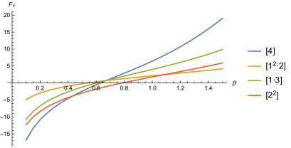
(b) $|Y|=4$

Figure 2: Plot of $F_{Y}(\beta)$ for 2(a) $|Y|=3$ and 2(b) $|Y|=4$ with $N=60$. Note that the horizontal axis is $\beta^{\prime}=\beta/N^{2/3}$.

When the temperature is below the RSB transition $T<T_{\text{RSB}}$, the totally connected contribution $Y=[n]$ becomes dominant. One can see this explicitly for $n=3,4$ in Figure 2: the blue curve labeled by $Y=[n]$ becomes the largest contribution in the low temperature regime $\beta^{\prime}\gtrsim 1$. Thus we confirmed numerically the behavior claimed in (5).

3.4 Low temperature regime

In the previous subsection 3.3 we have seen that the totally connected part $\langle Z(\beta)^{n}\rangle_{c}$ becomes dominant in the low temperature regime $T<T_{\text{RSB}}$. We find that in this regime $\langle Z(\beta)^{n}\rangle_{c}$ is further approximated by the first term in (17) and (18)

$$\langle Z(\beta)^{n}\rangle_{c}\approx\operatorname{Tr}A(n\beta)=\langle Z(n\beta)\rangle,\quad(T<T_{\text{RSB}}).$$ (49)

To see this, let us consider the ratio $r_{n}(\beta)$ between the both sides of (49)

$$r_{n}(\beta)=\frac{\langle Z(\beta)^{n}\rangle_{c}}{\langle Z(n\beta)\rangle}.$$ (50)

In Figure 3, we plot $r_{n}(\beta)$ for $n=2,3,4$ as a function of $\beta^{\prime}=\beta/N^{2/3}$ for $N=60$ (red curve) and $N=100$ (blue dots). As we can see from Figure 3, $r_{n}(\beta)$ approaches $1$ as $\beta^{\prime}$ increases, which confirms the claim in (49). Finally, combining (49) and (5), in the low temperature regime we find

$$\langle Z(\beta)^{n}\rangle\approx\langle Z(\beta)^{n}\rangle_{c}\approx\langle Z(n\beta)\rangle,\qquad(T<T_{\text{RSB}}).$$ (51)

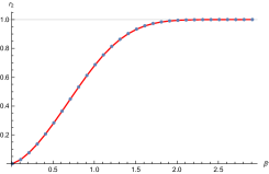
(a) $r_{2}(\beta)$

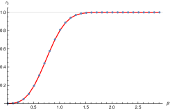
(b) $r_{3}(\beta)$

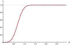
(c) $r_{4}(\beta)$

Figure 3: Plot of $r_{n}(\beta)$ for 3(a) $n=2$, 3(b) $n=3$, and 3(c) $n=4$. Note that the horizontal axis is $\beta^{\prime}=\beta/N^{2/3}$. The red curve is the plot for $N=60$, while the blue dots represent the value of $r_{n}(\beta)$ for $N=100$.

4 Possible implications for multiply-coupled SYK models

In this section, we will discuss possible implications of our findings in the GUE random matrix model for multiply-coupled SYK models and their dual JT gravity.

The SYK model exhibits a chaotic behavior which is diagnosed by the SFF Cotler:2016fpe as well as the out-of-time ordered correlators (OTOCs) kitaev ; Maldacena:2016hyu ; Kitaev:2017awl . The Lyapunov exponent extracted from the OTOC of SYK model saturates the chaos bound bound which is consistent with the holographically dual black hole interpretation.

The level statistics of energy eigenvalues of the SYK model is well approximated by the random matrix models Garcia-Garcia:2016mno ; Cotler:2016fpe , which is also a characteristic feature of the quantum chaos. At low energy, the SYK model is described by the Schwarzian theory whose density of states is given by Garcia-Garcia:2017pzl ; Stanford:2017thb

$$\rho_{\text{Sch}}(\mathcal{E})=\sinh(2\pi\sqrt{\mathcal{E}}).$$ (52)

Although this is different from the simple semi-circle law in (19), $\rho_{\text{Sch}}(\mathcal{E})$ exhibits the same square-root behavior $\rho(\mathcal{E})\sim\sqrt{\mathcal{E}}$ (40) near the edge of the spectrum $\mathcal{E}=0$.

The above discussion suggests that the RSB transition observed in the GUE random matrix model in the previous section 3 also appears in the multiply-coupled SYK models, where the expectation value of $\langle Z(\beta)^{n}\rangle$ is taken by the disorder average over the random coupling in the Hamiltonian of SYK model. Recall that the scaling of the effective string coupling $g_{\text{eff}}$ in (34) is sensitive only to the behavior of eigenvalue density near the edge of the spectrum. Thus the behavior of $g_{\text{eff}}$ is expected to be the same for both the GUE random matrix model and the Schwarzian theory, and the transition occurs when $g_{\text{eff}}\sim 1$.

However, the RSB and the role of replica non-diagonal saddle point in the SYK model are still controversial Gur-Ari:2018okm ; Wang:2018ijz ; Saad:2018bqo ; Arefeva:2018vfp ; It is argued in Gur-Ari:2018okm that RSB does not occur in the SYK model. In Wang:2018ijz ; Saad:2018bqo ; Arefeva:2018vfp the replica non-diagonal saddle points are found by numerical analysis but it is argued that such saddle points are always sub-dominant compared to the diagonal one. In a recent paper SSS , it is argued that a non-perturbative completion of Schwarzian theory and its dual JT gravity is given by a certain double-scaled matrix model, and it is suggested that the replica non-diagonal saddle point does play an essential role.

Interestingly, it is shown in Qi that by turning on a mass term connecting the fermions living on different replicas, the partition function of coupled SYM models exhibits a first order phase transition, which is very similar to the transition we observed for $\langle Z(\beta)^{2}\rangle$ in the GUE random matrix model (see also Kim:2019upg for the symmetry breaking in coupled SYK models).

In the rest of this section, we will have in mind a certain soft breaking of replica symmetry as in Qi , and see what kind of dual gravity picture is expected based on the observation in the previous section 3. Our argument is merely a heuristic one and we have not performed an actual calculation of the multiply-coupled SYK models with $n\geq 3$ replicas generalizing Qi . It would be very interesting to study such multiply-coupled SYK models.

Based on the fact that the level statistics of the SYK model is described by a random matrix model, we expect that the phase structure of the GUE random matrix model we observed in the previous section captures the essential part of the low energy dynamics of multiply-coupled SYK models.

4.1 Wormhole networks

The bulk gravity picture of $n=2$ coupled SYK models in Qi is that the two terms in the expansion of $\langle Z(\beta)^{2}\rangle$ in (9) correspond to the two geometries with different topology: the first term $\langle Z(\beta)\rangle^{2}$ corresponds to the two disconnected disks associated with the two Euclidean black holes, while the second term $\langle Z(\beta)^{2}\rangle_{c}$ corresponds to the Euclidean wormhole connecting the two boundaries with the topology of annulus. This is depicted schematically as:

$$\begin{aligned} \langle Z(\beta)^{2}\rangle&=\langle Z(\beta)\rangle^{2}\quad+\quad\langle Z(\beta)^{2}\rangle_{c}\\ &=\leavevmode\hbox to33.41pt{\vbox to17.47pt{\text{[drawing]}}}\hskip 14.22636pt+\hskip 14.22636pt\leavevmode\hbox to33.41pt{\vbox to17.47pt{\text{[drawing]}}}\quad.\end{aligned}$$ (53)

This picture for $n=2$ replicas suggests that the holographic dual geometry of the connected correlator is literally connected by an Euclidean wormhole, in the same spirit as the ER=EPR conjecture Maldacena:2013xja . Assuming this interpretation, we can draw a cartoon of spacetime geometry for all terms $\mathcal{Z}_{Y}(\beta)$ in the expansion (11). For $n=3$ we have three terms $Y=[1^{3}],[1\cdot 2],[3]$ in the expansion (9), where the corresponding spacetime geometries look like

$$\mathcal{Z}_{[1^{3}]}(\beta)=\langle Z(\beta)\rangle^{3}=\quad\leavevmode\hbox to35.75pt{\vbox to32.04pt{\text{[drawing]}}}\quad,$$ (54)

$$\mathcal{Z}_{[1\cdot 2]}(\beta)=3\langle Z(\beta)\rangle\langle Z(\beta)^{2}\rangle_{c}=\quad\leavevmode\hbox to35.75pt{\vbox to32.04pt{\text{[drawing]}}}\quad+\quad\leavevmode\hbox to35.75pt{\vbox to32.04pt{\text{[drawing]}}}\quad+\quad\leavevmode\hbox to35.75pt{\vbox to32.04pt{\text{[drawing]}}}\quad,$$ (55)

and

$$\mathcal{Z}_{[3]}(\beta)=\langle Z(\beta)^{3}\rangle_{c}=\quad\leavevmode\hbox to35.75pt{\vbox to32.04pt{\text{[drawing]}}}\quad.$$ (56)

Note that the coefficient $3$ in $\mathcal{Z}_{[1\cdot 2]}(\beta)=3\langle Z(\beta)\rangle\langle Z(\beta)^{2}\rangle_{c}$ has a natural interpretation as the number of ways to connect two boundaries by a wormhole out of three boundaries, as shown in (55). One can also check that the coefficient appearing in the expansion of $\langle Z(\beta)^{4}\rangle$ in (9) has a similar interpretation.

For general $n$, from the result of random matrix model in (5), we can draw the following dual spacetime picture: at high temperature $T>T_{\text{RSB}}$ the bulk geometry is $n$ disconnected disks representing $n$ disconnected Euclidean black holes, while at low temperature $T<T_{\text{RSB}}$ the corresponding bulk geometry is an $n$-pronged wormhole connecting the $n$ boundaries (see (56) for the example of three-pronged wormhole). Around the RSB transition temperature $T\sim T_{\text{RSB}}$, we speculate that the dual gravity side does not correspond to a classical geometry, but it is described by a superposition of random wormhole networks. It would be very interesting to understand the implication of this RSB transition in the bulk gravity theory.

4.2 Thermofield $n$-tuple and ground state

In the previous section 3.4, we observed that $\langle Z(\beta)^{n}\rangle$ is reduced to $\langle Z(\beta)^{n}\rangle_{c}\approx\langle Z(n\beta)\rangle$ in the low temperature regime (51). Let us consider a possible interpretation of this behavior. We first notice that our starting point $Z(\beta)^{n}$ is written as a trace over the $n$-th power of the Hilbert space $\mathcal{H}$ of a single system

$$Z(\beta)^{n}=\operatorname{Tr}_{\mathcal{H}^{\otimes n}}\underbrace{e^{-\beta H}\otimes\cdots\otimes e^{-\beta H}}_{n}~{}.$$ (57)

Since $Z(\beta)^{n}$ is defined as a trace in $\mathcal{H}^{\otimes n}$, it is natural to express its low temperature limit $\langle Z(n\beta)\rangle$ in (51) as a quantity involving $\mathcal{H}^{\otimes n}$. However, this seems impossible since $Z(n\beta)=\operatorname{Tr}_{\mathcal{H}}e^{-n\beta H}$ is a trace on the single Hilbert space $\mathcal{H}$. This tension is resolved by assuming that the low temperature state in $\mathcal{H}^{\otimes n}$ is highly entangled. We propose that $\langle Z(n\beta)\rangle$ should be written as

$$\langle Z(n\beta)\rangle=\langle\text{TF}_{n}|\text{TF}_{n}\rangle,$$ (58)

where $|\text{TF}_{n}\rangle$ denotes the “thermofield $n$-tuple state”

$$|\text{TF}_{n}\rangle=\sum_{i}e^{-\frac{n\beta}{2}E_{i}}\underbrace{|i\rangle\otimes\cdots\otimes|i\rangle}_{n}~{}~{}\in\mathcal{H}^{\otimes n}.$$ (59)

This is a generalization of the thermofield double state $|\text{TFD}\rangle$ for $n=2$

$$|\text{TFD}\rangle=|\text{TF}_{2}\rangle.$$ (60)

In the low temperature limit, the partition function is approximated by the expectation value in the ground state. From (51) and (58), we expect that the ground state $|\Psi_{\text{gnd}}\rangle$ of multiply-coupled system is approximated by the thermofield $n$-tuple state

$$|\Psi_{\text{gnd}}\rangle\approx|\text{TF}_{n}\rangle.$$ (61)

This property is indeed observed for $n=2$ in Qi .

Our relations (51) and (58) are also consistent with the picture of spacetime geometry built by entanglement VanRaamsdonk:2010pw and the ER=EPR conjecture Maldacena:2013xja . In fact, the relation between the thermofield double state $|\text{TFD}\rangle$ and the wormhole picture of $\langle Z(\beta)^{2}\rangle_{c}$ depicted in (53) is the motivation for the proposal in VanRaamsdonk:2010pw ; Maldacena:2013xja . Then it is natural to generalize this picture to the case of multiple boundaries. For instance, the thermofield triple state $|\text{TF}_{3}\rangle$ corresponds to the three-pronged wormhole depicted in (56). We emphasize that only the totally connected part is dominant in the low temperature limit, and hence the ground state $|\Psi_{\text{gnd}}\rangle\approx|\text{TF}_{n}\rangle$ would be dual to an $n$-pronged wormhole. In the spirit of VanRaamsdonk:2010pw ; Maldacena:2013xja , this $n$-pronged wormhole can be thought of as a geometric manifestation of the entanglement in the state (59).

- (1) D. Sherrington and S. Kirkpatrick, “Solvable Model of a Spin-Glass,” Phys. Rev. Lett. 35, 1792 (1975).
- (2) G. Parisi, “Infinite Number of Order Parameters for Spin-Glasses,” Phys. Rev. Lett. 43, 1754 (1979).
- (3) G. Parisi, “A sequence of approximated solutions to the S-K model for spin glasses,” J. Phys. A 13, L115 (1980).
- (4) F. Denef, “TASI lectures on complex structures,” TASI 2010, arXiv:1104.0254 [hep-th].
- (5) A. Kamenev and M. Mezard, “Wigner-Dyson Statistics from the Replica Method,” J. Phys. A 32, 4373-4388 (1999), [cond-mat/9901110].
- (6) B. Derrida, “Random-energy model: An exactly solvable model of disordered systems,” Phys. Rev. B 24, 2613 (1981).
- (7) P. H. Ginsparg and G. W. Moore, “Lectures on 2-D gravity and 2-D string theory,” [hep-th/9304011].
- (8) A. Kitaev, “A simple model of quantum holography (part 1 and 2),” Talks at KITP on April 7, 2015 and May 27, 2015.
- (9) J. Maldacena and D. Stanford, “Remarks on the Sachdev-Ye-Kitaev model,” Phys. Rev. D 94, no. 10, 106002 (2016), [arXiv:1604.07818 [hep-th]].
- (10) R. Jackiw, “Lower Dimensional Gravity,” Nucl. Phys. B 252, 343 (1985).
- (11) C. Teitelboim, “Gravitation and Hamiltonian Structure in Two Space-Time Dimensions,” Phys. Lett. 126B, 41 (1983).
- (12) A. Almheiri and J. Polchinski, “Models of AdS2 backreaction and holography,” JHEP 1511, 014 (2015), [arXiv:1402.6334 [hep-th]].
- (13) A. del Campo, J. Molina-Vilaplana and J. Sonner, “Scrambling the spectral form factor: unitarity constraints and exact results,” Phys. Rev. D 95, no. 12, 126008 (2017), [arXiv:1702.04350 [hep-th]].
- (14) K. Okuyama, “Spectral form factor and semi-circle law in the time direction,” JHEP 1902, 161 (2019), [arXiv:1811.09988 [hep-th]].
- (15) K. Okuyama, “Connected correlator of 1/2 BPS Wilson loops in SYM,” JHEP 1810, 037 (2018), [arXiv:1808.10161 [hep-th]].
- (16) M. L. Mehta, Random Matrices, Academic Press (2004).
- (17) J. K. Erickson, G. W. Semenoff and K. Zarembo, “Wilson loops in N=4 supersymmetric Yang-Mills theory,” Nucl. Phys. B 582, 155 (2000), [hep-th/0003055].
- (18) G. Akemann and P. H. Damgaard, “Wilson loops in =4 supersymmetric Yang-Mills theory from random matrix theory,” Phys. Lett. B 513, 179 (2001), Erratum: [Phys. Lett. B 524, 400 (2002)], [hep-th/0101225].
- (19) S. Giombi, V. Pestun and R. Ricci, “Notes on supersymmetric Wilson loops on a two-sphere,” JHEP 1007, 088 (2010), [arXiv:0905.0665 [hep-th]].
- (20) N. Drukker and D. J. Gross, “An Exact prediction of N=4 SUSYM theory for string theory,” J. Math. Phys. 42, 2896 (2001), [hep-th/0010274].
- (21) L. Leviandier, M. Lombardi, R. Jost and J. P. Pique, “Fourier Transform: A Tool to Measure Statistical Level Properties in Very Complex Spectra,” Phys. Rev. Lett. 56, 2449 (1986).
- (22) A. M. García-García and J. J. M. Verbaarschot, “Spectral and thermodynamic properties of the Sachdev-Ye-Kitaev model,” Phys. Rev. D 94, no. 12, 126010 (2016), [arXiv:1610.03816 [hep-th]].
- (23) J. S. Cotler, G. Gur-Ari, M. Hanada, J. Polchinski, P. Saad, S. H. Shenker, D. Stanford, A. Streicher and M. Tezuka, “Black Holes and Random Matrices,” JHEP 1705, 118 (2017), Erratum: [JHEP 1809, 002 (2018)], [arXiv:1611.04650 [hep-th]].
- (24) E. Witten, “Anti-de Sitter space, thermal phase transition, and confinement in gauge theories,” Adv. Theor. Math. Phys. 2, 505 (1998), [hep-th/9803131].
- (25) S. W. Hawking and D. N. Page, “Thermodynamics of Black Holes in anti-De Sitter Space,” Commun. Math. Phys. 87, 577 (1983).
- (26) O. Aharony, J. Marsano, S. Minwalla, K. Papadodimas and M. Van Raamsdonk, “A First order deconfinement transition in large N Yang-Mills theory on a small ,” Phys. Rev. D 71, 125018 (2005), [hep-th/0502149].
- (27) O. Aharony, J. Marsano, S. Minwalla, K. Papadodimas and M. Van Raamsdonk, “The Hagedorn - deconfinement phase transition in weakly coupled large N gauge theories,” Adv. Theor. Math. Phys. 8, 603 (2004), [hep-th/0310285].
- (28) A. Kitaev and S. J. Suh, “The soft mode in the Sachdev-Ye-Kitaev model and its gravity dual,” JHEP 1805, 183 (2018), [arXiv:1711.08467 [hep-th]].
- (29) J. Maldacena, S. H. Shenker and D. Stanford, “A bound on chaos,” JHEP 1608, 106 (2016), [arXiv:1503.01409 [hep-th]].
- (30) A. M. García-García and J. J. M. Verbaarschot, “Analytical Spectral Density of the Sachdev-Ye-Kitaev Model at finite N,” Phys. Rev. D 96, no. 6, 066012 (2017), [arXiv:1701.06593 [hep-th]].
- (31) D. Stanford and E. Witten, “Fermionic Localization of the Schwarzian Theory,” JHEP 1710, 008 (2017), [arXiv:1703.04612 [hep-th]].
- (32) G. Gur-Ari, R. Mahajan and A. Vaezi, “Does the SYK model have a spin glass phase?,” JHEP 1811, 070 (2018), [arXiv:1806.10145 [hep-th]].
- (33) I. Aref’eva, M. Khramtsov, M. Tikhanovskaya and I. Volovich, “Replica-nondiagonal solutions in the SYK model,” arXiv:1811.04831 [hep-th].
- (34) H. Wang, D. Bagrets, A. L. Chudnovskiy and A. Kamenev, “On the replica structure of Sachdev-Ye-Kitaev model,” arXiv:1812.02666 [hep-th].
- (35) P. Saad, S. H. Shenker and D. Stanford, “A semiclassical ramp in SYK and in gravity,” arXiv:1806.06840 [hep-th].
- (36) I. Aref’eva and I. Volovich, “Spontaneous symmetry breaking in fermionic random matrix model,” arXiv:1902.09970 [hep-th].
- (37) P. Saad, S. H. Shenker and D. Stanford, “JT gravity as a matrix integral,” arXiv:1903.11115 [hep-th].
- (38) J. Maldacena and X. L. Qi, “Eternal traversable wormhole,” arXiv:1804.00491 [hep-th].
- (39) J. Kim, I. R. Klebanov, G. Tarnopolsky and W. Zhao, “Symmetry Breaking in Coupled SYK or Tensor Models,” arXiv:1902.02287 [hep-th].
- (40) J. Maldacena and L. Susskind, “Cool horizons for entangled black holes,” Fortsch. Phys. 61, 781 (2013), [arXiv:1306.0533 [hep-th]].
- (41) M. Van Raamsdonk, “Building up spacetime with quantum entanglement,” Gen. Rel. Grav. 42, 2323 (2010), [Int. J. Mod. Phys. D 19, 2429 (2010)], [arXiv:1005.3035 [hep-th]].
- (42) R. P. Deane et al., “A close-pair binary in a distant triple supermassive black hole system,” Nature 511, 57-60 (2014).