New analytical tools for HDG in elasticity, with applications to elastodynamics
Abstract.
We present some new analytical tools for the error analysis of hybridizable discontinuous Galerkin (HDG) method for linear elasticity. These tools allow us to analyze more variants of HDG method using the projection-based approach, which renders the error analysis simple and concise. The key result is a tailored projection for the Lehrenfeld-Schöberl type HDG (HDG+ for simplicity) methods. By using the projection we recover the error estimates of HDG+ for steady-state and time-harmonic elasticity in a simpler analysis. We also present a semi-discrete (in space) HDG+ method for transient elastic waves and prove it is uniformly-in-time optimal convergent by using the projection-based error analysis. Numerical experiments supporting our analysis are presented at the end.
Key words and phrases:
discontinuous Galerkin method, hybridization, optimal convergence, elastic waves2010 Mathematics Subject Classification:
65N30, 65M60, 74B051. Introduction
The paper is devoted to present some new techniques for the a priori error analysis of a new class of hybridizable discontinuous Galerkin methods. The methods in this class use a special type of stabilization function that was first introduced by Lehrenfeld and Schöberl in [16]. We will call them HDG+ methods for simplicity. Instead of attempting to reach for maximal generality, we will focus on linear elasticity on tetrahedral meshes.
We begin by reviewing some existing works. The first HDG method for linear elasticity was proposed in [23]. The method enforces the symmetry of the stress strongly and uses order polynomial spaces for all variables. It was then proved in [13] that the method is optimal for displacement but only suboptimal for stress (order of ); they also showed the order is sharp on triangular meshes in the numerical experiments. To recover optimal convergence (based on which the superconvergence by post-processing is possible), there are mainly three approaches. The first approach relaxes the strong symmetry condition to weak symmetry [11]. In general, mixed finite element methods based on weak symmetric stress formulations are relatively easier to implement but use more degrees of freedom and therefore can be more costly to compute. The second and the third approaches are all based on strong symmetric stress formulations, where the conservation of angular momentum is automatically preserved. The second approach [4] uses -decomposition [5] to enrich the approximation space for stress by adding some basis functions. The approach recovers optimal convergence and also provides an associated tailor projection as an useful tool for error analysis. However, the added basis can be rational functions instead of polynomials and therefore can lead to some difficulties in implementation.
The focus of this paper is the third approach, which is to use HDG+ method for linear elasticity. The method was originally proposed in [16] for diffusion problems, then applied to steady-state linear elasticity in [19]. It uses only polynomial basis functions, achieves one order higher convergence rate for the displacement without post-processing, and its computational complexity is the same to the standard HDG method (order for both stress and displacement) for their global systems. However, the existing error analysis of HDG+ methods are all based on using orthogonal projections [15, 18, 19, 20, 21], which make the analysis slightly more complicated (it requires a bootstrapping argument to prove convergence of all variables, as opposed to consecutive energy and duality proofs), and detached from the existing projection-based error analysis of HDG methods [3, 6, 7, 8, 9, 10, 11, 14], where specifically constructed projections are used to make the analysis simple and concise. This motivates us to find a new kind of projection for HDG+ for elasticity. The goal of the projection is twofold: first of all, it takes care of all the off-diagonal terms in the matrix form of the equations (except for a block which is considered as a single diagonal term), and allows us to do a simple energy estimate for some of the variables; second, it facilitates a duality argument where the adjoint equation is fed with the missing error terms to estimate, by using the adjoint projection (consisting of a simple change of sign in the stabilization parameter ). This has been done in [12] for diffusion problems. A novelty of this paper is the fact that we complement the projection with an error term that does not affect the error bounds or the simplicity of their proofs. We have attached this error term to the projection to make the arguments simpler.
In summary, we have devised a projection for the HDG+ methods for linear elasticity. The projection enables us to: (1) recycle existing projection-based error analysis techniques for the analysis of HDG+ methods; (2) make the error analyis simple and concise; (3) build connections between -decompositions [4, 5] and HDG+ methods. To be more specific, we present a semi-discrete HDG+ method for transient elastic waves that has a uniform-in-time optimal convergence. We show that the proof for optimal convergence can be easily obtained by using the new projection and some existing techniques in traditional HDG methods for evolutionary equations [6]. Moreover, we recover the error estimates for steady-state elasticity [19] and frequency domain elastodynamics [15] by using the projection-based analysis, and we show that the analysis can be simplified in both cases. Since the construction of the HDG+ projection involves first constructing a projection associated to an -decomposition, it also shed some light upon the connections between these two kinds of methods.
To provide a more intuitive view, we put the main procedures of constructing the projection in the flow chart Figure 1.
The associated boundary remainder term related to the projection behaves like interpolation error and it depends only on the local projection. As we will see later in the applications, the boundary remainder together with the stabilization parameter play a key role in the optimal convergence of the HDG+ methods, allowing us more flexibility, since now we only need to find a projection such that its associated boundary remainder is small enough to guarantee optimal convergence, instead of enforcing it to vanish, which is the case of the standard projection.
The rest of the paper is organized as follows. In Section 2, we present the main theorem about the projection and its properties. In Section 3, we show the procedures for constructing the projection on the reference element. In Section 4, we develop a systematic approach of changes of variables to obtain the projection on the physical element. In Section 5 and 6, we recover the error estimates in steady-state elasticity [19] and elasto-dynamics [15] using projection-based analysis. In Section 7, we present a semi-discrete HDG method for transient elastic waves and prove it is optimally convergent, uniformly in the time variable. Finally, we give some numerical experiments to support our analysis.
2. The projection
Since the main tool and one of the principal novelties of this article is the new HDG projection for elasticity, we first introduce its main properties in Theorem 2.1. The reader just interested in the applications can skip the sections devoted to its construction and analysis (Section 3 and 4) and jump directly to how it is used (Section 5, 6 and 7). To speed up the introduction of the projection we give a quick notation list to be used throughout the article.
-
•
For a domain , the respective inner products of and will be denoted
where in the latter the colon denotes the Frobenius product of matrices and is the space of symmetric matrices. The norm of both spaces will be denoted .
-
•
For a Lipschitz domain , the inner product in will be denoted
and the associated norm will be denoted .
-
•
The Sobolev seminorm in and will be denoted .
-
•
The symmetric gradient operator (linearized strain) is given by
and the divergence operator will be applied to symmetric-matrix-valued functions by acting on their rows, outputting a column vector-valued function.
-
•
When is a Lipschitz domain, we will consider the space
and the normal traction operator defined by Betti’s formula
Here is the trace operator, is the dual space of , and the angled bracket denotes their duality product that extends the inner product.
For discretization we will consider a sequence of tetrahedral meshes and the following notation:
-
•
is a tetrahedron, of diameter and inradius at most for a fixed shape-regularity constant .
-
•
is the set of faces of .
-
•
is the space of -valued polynomial functions of degree up to , where .
-
•
is the space of piecewise polynomial functions on the boundary of , with as above.
-
•
is the orthogonal projection onto the image space, with as above.
-
•
is the orthogonal projection onto the image space. This operator will often be applied on the trace of a function in on .
-
•
is a so-called stabilization function satisfying
(2.1) for fixed positive constants and , independent of (i.e., of the particular mesh).
-
•
The wiggled inequality sign hides a constant that is independent of , while means .
Theorem 2.1.
For , there exists a family of projections and associated boundary remainder operators
depending on , where is a constant positive definite matrix on each face of , and if and , the following conditions hold:
| (2.2a) | ||||||
| (2.2b) | ||||||
| (2.2c) | ||||||
Moreover, if satisfies (2.1) and with , then we have the estimates:
| (2.3) |
The constant depends only on the polynomial degree , the constants and in (2.1) and the shape-regularity constant . Finally, the ‘adjoint’ projection can be defined as
| (2.4) |
This projection satisfies the properties (2.2) with the same , if we substitute by .
3. The projection in the reference element
3.1. Preparatory work on the reference element
In this section we will work on the reference tetrahedron . The trace for vector-valued functions on the reference element will be denoted , and the normal traction operator on the reference element will be denoted . We will use shortened notation for the following spaces:
| (3.1a) | |||||
| (3.1b) | |||||
A new space will be defined once we have introduced some tools for it. Note that these constructions can be done directly on any tetrahedron [4].
The first of these constructions is a lifting of the traction operator. It will act on the space
where is the six-dimensional space of infinitesimal rigid motions
Note that the trace space of is also six-dimensional, i.e., if vanishes on the boundary of , then . We thus define the operator by
| (3.2a) | ||||
| (3.2b) | ||||
or equivalently
| (3.3a) | ||||
| (3.3b) | ||||
The definition (3.2) is correct since it involves the solution of a coercive variational problem on a quotient space, due to Korn’s Second Inequality. From (3.3) it is clear that
| (3.4) |
We next consider the spaces
and
Theorem 3.1.
The following properties hold:
-
(a)
for all ,
-
(b)
is an isomorphism between and , and its inverse is ,
-
(c)
,
-
(d)
with orthogonal sum.
Proof.
Properties (a) and (b) are easy consequences of (3.4). By (a), and, therefore, if , then (the latter two sets are orthogonal to each other by definition of ), but then (b) proves that , which proves (c). Finally, if and , then
which shows that the sum is orthogonal. Since is the orthogonal complement of the latter set, (d) is proved. ∎
The Cockburn-Fu discrete pair for elasticity [4] is given by the spaces
(the sum is direct because of Theorem 3.1) and . In their context of -decompositions for elasticity, the following result is a key one, that we will need to work with our extended pair .
Theorem 3.2.
The following properties hold:
-
(a)
,
-
(b)
,
-
(c)
,
-
(d)
where the orthogonal complement is taken in , while is taken in ,
-
(e)
, with orthogonal sum,
-
(f)
The map is an isomorphism.
Proof.
Property (a) follows by definition and (b) is a simple consequence of Theorem 3.1(a). To show (c), note simply that , while all other elements are polynomials of degree less than or equal to .
To prove (d) to (f), it will be convenient to identify the set
| (3.5) |
which appeared in the definition of (3.1).
By Theorem 3.1(d) and (3.5), we have
| (3.6) |
Using the definitions of we have
| (3.7) |
where in the last equality we have applied that is onto (this is easy to prove), its kernel is , and the kernel of is . The equalities (3.6) and (3.7) prove (d).
Due to parts (a) and (b) of this theorem, we have
which proves that the sum of and is orthogonal. Since is injective (this result is known; see, for instance, [22] and [12]), the property (e) will follow from having proved that is injective.
We first prove the following technical result: if satisfies and , then , i.e., the component in vanishes. To do that, take and note that Theorem 3.1(a) shows that if , then . Since
by Theorem 3.1(d), it follows that , which proves that by Theorem 3.1(b).
The proof of injectivity of is then simple. If satisfies , then by part (a)
and, taking (by part (b)), we prove that . Therefore, and hence . This completes the proof of (e) and (f). ∎
For the rest of this section we fix the stabilization parameter such that
| (3.8) |
3.2. A projection on an extended space
Given , we look for
| (3.9a) | |||||
| satisfying | |||||
| (3.9b) | |||||
| (3.9c) | |||||
| (3.9d) | |||||
| (3.9e) | |||||
where is the orthogonal complement of in . Note that (3.9e) is equivalent to
and, since and , equations (3.9c) and (3.9d) imply that we can substitute (3.9e) by the condition
| (3.10) |
which contains redundant restrictions already imposed in the other equations. Note also that the projection can be eliminated in (3.9d) but not in (3.9e) or in (3.10), and that the bilinear form
is symmetric, bounded, and positive semi-definite in . We next prove that is actually a well-defined projection onto .
Proposition 3.3.
The process of defining the projection in (3.9) is equivalent to a square invertible linear system.
Proof.
Note first that by Theorem 3.2(d)
which proves that (3.9) is equivalent to a linear system with as many equations as unknowns. We thus only need to prove uniqueness of solution.
A homogeneous solution of (3.9) is a pair satisfying (recall how (3.10) is a consequence of (3.9))
| (3.11a) | |||||
| (3.11b) | |||||
| (3.11c) | |||||
| (3.11d) | |||||
We now take (with the complement in ; also see (3.11a)) in (3.11d), recalling that (cf. Theorem 3.2(b)) and obtain
This argument uses that is piecewise constant, so that multiplication by is an endomorphism in . Since is positive definite on each face, this proves that .
Looking at the proof of Proposition 3.3, it is clear that we could have also defined the projection for any such that is negative definite on each face.
Proposition 3.4 (Stability).
For any and , there exists such that if , then
| (3.12) |
whenever satisfies
| (3.13) |
Proof.
Numbering the faces of and the entries of a symmetric matrix with indices from one to six, we can identify . We can thus make the identification
where is an open set. We can also identify
where is compact. To be more specific, we can write the identification as follows:
where satisfies that is supported on the -th face () and its -th entry () in is equal to and the rest of the entries are all equal to .
Consider now the continuous trial and test spaces
and their discrete counterparts
We can define bilinear forms
as follows:
We can see that are all bounded -independent (but dependent on through the operator ) bilinear forms. Then equations (3.9) can be rephrased in the following form: given , find such that
| (3.14) |
Equations (3.14) are uniquely solvable for every (this is a restatement of Proposition 3.3) and define a bounded linear operator The function , from to the space of bounded linear operators from to , is rational and therefore bounded on the compact set . We can thus bound
| (3.15) |
where is any norm we choose in . If we select the norm
A simple argument shows that algebraic condition (3.13) is equivalent to asking that the spectrum of is contained in for all and also to the inequality
| (3.16) |
3.3. The projection and the remainder
Let now be the orthogonal projection onto . For we define
| (3.17a) | |||
| where | |||
| (3.17b) | |||
Since , it follows that for all and therefore
| (3.18) |
In particular, is a projection onto . Note that we do not give a set of equations to define , which is given as the application of followed by an orthogonal projection applied to the first component of the output. However, the following equations relate the projection and the associated remainder .
Proposition 3.5.
Let satisfy (3.8), then and satisfy
| (3.19a) | ||||||
| (3.19b) | ||||||
| (3.19c) | ||||||
Proof.
Following the definition (3.17), we introduce the intermediate projection so that and .
Proposition 3.6 (Estimate in the reference element).
Proof.
Let . Note that (this is obvious from the equations that define , namely (3.9)) and therefore
By Proposition 3.4, we have
for some constant depending only on , and . Since is bounded, there exists a constant such that
Taking now and , and applying (3.18) to the pair , we have
and
Note that is the projection onto . Therefore, there exists a constant such that
Finally, notice that . The result follows now by a compactness argument (Bramble-Hilbert lemma). ∎
4. The projection in the physical elements
4.1. Pull-backs and push-forwards
In this section we derive a systematic approach to changes of variables for vector- and matrix-valued functions from a general shape-regular tetrahedron to the reference element. The language mimics that of [22] (or [12]). Let be a tetrahedron and be an invertible affine map from the reference element to . We will denote and . We also consider the piecewise constant function such that for all integrable ,
The trace and normal trace operators on will be denoted and . Given
we define
where . The following properties are easy to prove.
Proposition 4.1 (Change of variables in integrals).
We have the following identities
| (4.1a) | ||||||
| (4.1b) | ||||||
| (4.1c) | ||||||
The next group of results about changes of variables involve the interaction of integrals with differential operators or trace operators.
Proposition 4.2 (Change of variables in bilinear forms).
We have the following indentities:
| (4.2a) | |||||||
| (4.2b) | |||||||
| (4.2c) | |||||||
| (4.2d) | |||||||
| (4.2e) | |||||||
| (4.2f) | |||||||
Here and
| (4.3) |
Proof.
Using the definitions, it is easy to prove that
| (4.4) |
Then (4.2a), (4.2e), and (4.2f) are easy consequences of Proposition 4.1. Let now and . Using implicit summation for repeated indices, we have for each
and therefore . This and (4.1a) prove (4.2b). Note next that, using identities we have already proved and Proposition 4.1, we have
| (4.5a) | ||||
| (4.5b) | ||||
and (4.2c) is thus proved. Since is dense in , (4.2d) follows from (4.2c). ∎
The final result of this section contains all scaling inequalities. Shape-regularity can be rephrased as the asymptotic equivalences (recall that we are in three dimensions)
| (4.6) |
Therefore
| (4.7) |
For the hat transformations, we have the following scaling rules, which can be easily proved using (4.6), (4.7), and the chain rule.
Proposition 4.3 (Scaling equivalences).
With hidden constants depending on shape-regularity and on , we have
| (4.8a) | ||||||
| (4.8b) | ||||||
| (4.8c) | ||||||
4.2. The projection and the remainder on
Consider the spaces
The projection and the remainder are defined by a pull-back process: given , we define
| (4.9a) | ||||
| by the relations | ||||
| (4.9b) | ||||
| (4.9c) | ||||
We now prove Theorem 2.1. We start by proving a technical lemma, continue showing that equations (2.2) hold (we present this as Proposition 4.5), and finish by proving the estimates (2.3).
Lemma 4.4.
Proof.
Proposition 4.5.
Assume that satisfies
If and , then the following equations hold:
| (4.11a) | ||||||
| (4.11b) | ||||||
| (4.11c) | ||||||
Proof.
Assume now that is of order , as expressed in (2.1). By (4.6) and Proposition 4.3 we can write (take for )
| (4.12) |
where and are constants related to shape-regularity of . We are now ready to apply Proposition 3.6 with , and (compare (4.12) with (3.16)). Using the definition of the projection (4.9), Proposition 4.3 for the scaling properties, and Proposition 3.6 for the estimates, we have
and (2.3) is thus proved.
5. Steady-state elasticity
5.1. Method and convergence estimates
From now on, we shift our attention from the construction of the projection to its applications. We begin by introducing more notation for the rest of the paper. Let be a Lipschitz polyhedral domain in . We denote the compliance tensor by , where is the space of linear maps from to itself. We assume for some positive constant , and is uniformly symmetric and positive almost everywhere on , i.e., there exists such that for almost all ,
Let be a family of conforming tetrahedral partitions of , which we assume to be shape-regular. Namely, there exists a fixed constant , such that for all , where denotes the inradius of . We denote as the mesh size and set the following discrete spaces:
The related discrete inner products are denoted as
Finally, we use the following notation for the discrete and the weighted discrete norms:
where or , and or . Here is the stabilization function which we assume to satisfy (2.1) on every element .
In this section, we give a projection-based error analysis to the HDG+ method introduced in [19]. We will show that the analysis can be simplified by using Theorem 2.1. To begin with, we review the steady-state linear elasticity equations:
| (5.1a) | ||||||
| (5.1b) | ||||||
| (5.1c) | ||||||
where and . The HDG+ method for (5.1) is: find such that
| (5.2a) | ||||||
| (5.2b) | ||||||
| (5.2c) | ||||||
| (5.2d) | ||||||
Since we will use a duality argument to estimate the convergence of , here we write down the adjoint equations for (5.1):
| (5.3a) | ||||||
| (5.3b) | ||||||
| (5.3c) | ||||||
with input data , and we assume the additional elliptic regularity estimate
| (5.4) |
where is a constant depending only on and . The following convergence theorem will be proved in Subsection 5.2.
Theorem 5.1.
For and , we have
If (5.4) holds, then we also have
Here, depends only on the polynomial degree and the shape-regularity of , while depends also on and .
Note that in [19, Theorem 2.1] the meshes are assumed to be quasi-uniform, whereas here we only require to be shape-regular.
5.2. Proof of Theorem 5.1
To begin with, we use the element-by-element projection defined in (4.9) (we will only use Theorem 2.1, not the definition) on the solution :
and define the error terms and the approximation terms:
We aim to control the terms () by the terms () and .
Proposition 5.2 (Energy estimate).
The following energy identity holds
| (5.5) |
Consequently,
| (5.6) |
Proof.
The proof here will be similar to the proof of [7, Lemma 3.1 & 3.2]. By Theorem 2.1, we first obtain a set of projection equations satisfied by , and . We then subtract (5.2) from the projection equations and obtain the following error equations:
| (5.7a) | ||||
| (5.7b) | ||||
| (5.7c) | ||||
| (5.7d) | ||||
| (5.8) |
Now taking in (5.7a), in (5.7b), and then adding (5.7a), (5.7b) and (5.8), we obtain the energy identity (5.5), from which the estimate (5.6) follows easily. ∎
Proposition 5.3 (Estimate by duality).
Proof.
The proof here will be similar to the proof of [7, Lemma 4.1 & Theorem 4.1]. Consider the adjoint equations (5.3). We take as the input data and apply the projection on with as the stabilization function. Namely,
By Theorem 2.1, , and satisfy
We now test the above equations with , and , then test the error equations (5.7) with , and . By comparing the two sets of equations, we obtain
After rearranging terms, we have
By Theorem 2.1 (with ) we have
By (2.5) we have
Finally, (2.1) implies
We next use (5.4) to control the term and use Proposition 5.2 to control the terms and . The proof is thus completed. ∎
6. Frequency-domain elastodynamics
6.1. Method and convergence estimates
In this section we give new proofs of error estimates to the second HDG+ method studied in [15] by using projection based analysis for the following time-harmonic linear elasticity problem
| (6.1a) | ||||||
| (6.1b) | ||||||
| (6.1c) | ||||||
where , , and denotes the density function. We assume that the wave number and is not a Dirichlet eigenvalue so that (6.1) is well-posed. Note that because of the different proof techniques, the dependence on the wave numbers of the error estimates will be different and not easy to compare. The emphasis here will be the simplified error analysis thanks to the introduction of the projection.
The HDG+ method for (6.1) is: find such that
| (6.2a) | ||||
| (6.2b) | ||||
| (6.2c) | ||||
| (6.2d) | ||||
for all , and . Here, the spaces , and are the same as those defined in Section 5.1 except now the functions contained in these spaces take complex values.
For , we assume that the solution to the adjoint equations for (6.1)
| (6.3a) | ||||||
| (6.3b) | ||||||
| (6.3c) | ||||||
satisfy
| (6.4) |
where we make the dependence on explicit for the constant . For the rest of this section, the wiggles sign will hide constants independent of and . We aim to prove the following theorem.
Theorem 6.1.
6.2. Proof of Theorem 6.1
Since the solution in (6.1) can take complex values, applying directly Theorem 2.1 is not feasible. However, this can be easily fixed by defining a new complex projection based on the original one: for , we define
| (6.5) |
It is easy to show that this complex projection also satisfies (2.2) and (2.3) (the only difference is that now the test functions in (2.2) can take complex values).
Similar to the beginning of Section 5.2, we first define the projections , the remainder term , the error , , , and approximation terms , .
Proposition 6.2 (Gårding-type identity).
The following energy identity holds
Consequently,
| (6.6) |
Proof.
By similar ideas used in the proof of Proposition 5.2, we obtain the following error equations:
| (6.7a) | ||||
| (6.7b) | ||||
| (6.7c) | ||||
| (6.7d) | ||||
for all , and . Taking , and , then adding the equations, we have the energy identity.
Denoting , and applying the Cauchy-Schwarz inequality on the identity, we have
The estimate (6.6) now follows by using Young’s inequality. ∎
Proposition 6.3 (Estimate by bootstrapping).
Suppose and (6.4) holds. If is small enough, then
Proof.
Consider the adjoint equations (6.3) and take . Following similar ideas in the proof of Proposition 5.3, we first apply the projection on with stabilization function to obtain the projection equations (about ). We next test the projection equations with , and , test the error equations (6.7) with , and , and compare the two sets of equations. Then we obtain (define and for convenience)
After rearranging terms, we have
| (6.8) |
By Theorem 2.1 (with ), we have
and also
By (2.5) we have . Now we use (6.4) in (6.8) to obtain
Next we use (6.6) and bound
Therefore, when is small enough, we have
The first inequality is thus proved. The second inequality can be proved by combining (6.6) and the above inequality. ∎
7. Transient elastodynamics
7.1. The semi-discrete HDG+ method
In this section, we present a semi-discrete (in space) HDG+ method for transient elastic waves and prove it is uniformly-in-time optimal convergent. The equations we consider are
| (7.1a) | ||||||
| (7.1b) | ||||||
| (7.1c) | ||||||
| (7.1d) | ||||||
| (7.1e) | ||||||
where and . For the initial conditions, we assume .
The HDG+ method for (7.1) looks for
such that for all
| (7.2a) | ||||
| (7.2b) | ||||
| (7.2c) | ||||
| (7.2d) | ||||
for all , and . For the initial conditions of the method, we use ideas from [6]. The initial velocity is defined by using the projection in Theorem 2.1
| (7.3) |
and the initial displacement is defined to be the solution of the HDG+ discretization of the steady-state system
| (7.4a) | ||||||
| (7.4b) | ||||||
| (7.4c) | ||||||
Namely, we find such that
| (7.5a) | ||||
| (7.5b) | ||||
| (7.5c) | ||||
| (7.5d) | ||||
for all . For notational convenience, we define the following space-time norms
where can be replaced by , , , , , , or . The parameter takes values in , and when , we consider the supreme norm in time instead of integration. Now we define the projections and the remainder terms for all :
The related error and approximation terms (for all ) are denoted
For the rest of this section, the wiggles sign will hide constants independent of and . The main results in this section are Theorems 7.1 and 7.2.
Theorem 7.1.
For , the following estimates hold
For the next theorem, we need to assume that the elliptic regularity condition
| (7.6) |
holds for any such that the right hand side of the above inequality is finite. Note that (7.6) is the same as (5.4). We rephrase it here to have it in the form we will use it.
Theorem 7.2.
We next give the proofs for the above two theorems in the following two subsections respectively.
7.2. Energy estimates
In this subsection, we give a proof to Theorem 7.1. We first present two lemmas, which give the error equations when and the error equations when , respectively.
Lemma 7.3.
For all , the following error equations
| (7.7a) | ||||
| (7.7b) | ||||
| (7.7c) | ||||
| (7.7d) | ||||
| (7.7e) | ||||
| (7.7f) | ||||
hold for all .
Lemma 7.4.
The following error equations
| (7.8a) | ||||
| (7.8b) | ||||
| (7.8c) | ||||
| (7.8d) | ||||
hold for all .
The next proposition gives estimates to the error terms when .
Proposition 7.5.
The following estimates hold:
| (7.9) | ||||
| (7.10) | ||||
| (7.11) |
Proof.
Taking , and in the error equations (7.8) and adding the equations, we have
The first estimate (7.9) then follows from the latter identity.
Note that the boundary remainder operator defined in Theorem 2.1 is linear, thus commuting with the time derivative
This commutativity holds for the projection as well for similar reasons.
Proposition 7.6.
For , we have
| (7.12) | ||||
| (7.13) |
Proof.
Taking the first order derivative of (7.7a) and testing it with , then choosing in (7.7b) and in (7.7c), and finally taking the first order derivative of (7.7d) then adding the equations, we obtain (7.12).
Taking the second order derivative of (7.7a) and testing it with , then taking the first order derivative of (7.7b) and testing it with , taking the first order derivative of (7.7c) and testing it with , and finally taking the second order derivative of (7.7d) and adding the equations, we obtain (7.13). ∎
The final ingredient we need is a Grönwall type inequality.
Lemma 7.7.
Suppose are continuous and positive functions defined on and is a constant. If
then
Proof.
Consider the interval and let maximize in the interval. Then we have
∎
7.3. Duality argument
In this subsection, we give a proof to Theorem 7.2 by using the duality argument. To begin with, we consider the adjoint equations of (7.1):
| (7.14a) | ||||||
| (7.14b) | ||||||
| (7.14c) | ||||||
| (7.14d) | ||||||
| (7.14e) | ||||||
For a time-dependent function , we write
The following proposition allows us to control the solution of (7.14) in certain energy norms. Similar results can be found in [10].
Proposition 7.8.
Proof.
Now we define the dual projections and boundary remainder terms for the adjoint problem (7.14) (for all )
We also define the corresponding approximation terms
Proposition 7.9.
The following identity holds
where
Proof.
The next proposition gives an estimate for the term in Proposition 7.9.
Proposition 7.10.
If (7.6) holds, then
Proof.
In the coming arguments, for the sake of shortening some estimates, we will prove bounds in terms of the quantity
| (7.18) |
which we have shown in Proposition 7.8 that, assuming (7.6), we have the estimate
| (7.19) |
Note that
| (7.20) |
For the second term of (7.20), we have
We next estimate the remaining term in (7.20). Since for all , we have
where, is the -weighted projection onto . Testing the second error equation (7.7b) with we have
Now we use integration by part and obtain
Note that
Combining the above with the convergence properties about and (see Theorem 2.1) we have
Now back to the estimate of , we have
where we used the fact that for any . Finally, we use (7.19) to bound and the proof is completed. ∎
Now we are ready to prove Theorem 7.2.
Proof of Theorem 7.2.
Consider Proposition 7.9. We will give estimates for the terms for .
For , by (7.15) we have
Note that is the solution of the HDG+ scheme (7.5). By Theorem 5.1 in Section 5.1, we have
Therefore
For , we have
where we used the convergence properties about (by Theorem 2.1) and then equation (7.16) to bound (see (7.18) for the definition).
Using similar ideas, for we have
and for , we have
For , we simply use (7.15) and obtain
Now we use Proposition 7.10 to estimate , and finally obtain
Combing the above estimates with Proposition 7.5 and Theorem 7.1, the proof is completed.
∎
8. Numerical experiments
In this section, we present some numerical experiments to support our error estimates in Section 7. Note that there are experiments for the steady-state and time-harmonic cases in [19] and [15] respectively.
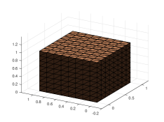
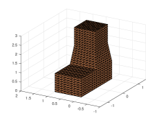
Convergence test. The experiments in this part are carried out on a cubic domain and a non-convex polyhedral domain (we will refer to it as the chimney; see Figure 2), the time interval is with , and we aim to estimate the relative errors
We consider a non-homogeneous isotropic material
with Lamé parameters
and the mass density is constant . As exact solution we take , where
and the temporal part is . The input data and are chosen so that (7.1) is satisfied. Note that we have chosen the exact solution that has vanishing initial conditions. This simplifies the calculations of and (they are automatically by (7.3) and (7.5)). When does not have vanishing initial conditions, the calculation of involves projecting to a space enriched by the -decomposition spaces (the Cockburn-Fu filling), which we have not found an easy way to implement. Finding easier ways of calculating for non-vanishing initial conditions will constitute our future works.
For the numerical schemes, we use the HDG+ method (7.2) for space discretization and Trapezoidal Rule Convolution Quadrature (TRCQ) (see [1, 17]) for time integration. This is equivalent to using Trapezoidal Rule time-stepping in the semidiscrete system. The time interval is equally divided and each timestep is of length . Since the error from the TRCQ is , we choose so that the error from the time discretization does not pollute the order of convergence of the space discretization.
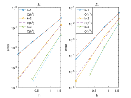
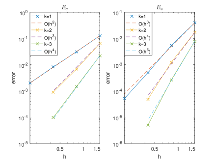
From Figure 3 or Table 1, we observe that the orders of convergence for and are and respectively, agreeing the estimates in Theorem 7.1 and Theorem 7.2.
| Cube | Chimney | ||||||||
| Error | Order | Error | Order | Error | Order | Error | Order | ||
| 1.6329 | 2.82E-1 | - | 4.32E-2 | - | 1.27E-1 | - | 3.93E-2 | - | |
| 1 | 0.8164 | 7.06E-2 | 2.00 | 6.16E-3 | 2.81 | 3.12E-2 | 2.02 | 5.36E-3 | 2.87 |
| 0.4082 | 1.93E-2 | 1.87 | 5.44E-4 | 3.50 | 8.16E-3 | 1.93 | 4.92E-4 | 3.44 | |
| 0.2041 | 4.79E-3 | 2.01 | 5.65E-5 | 3.27 | 1.99E-3 | 2.03 | 5.09E-5 | 3.28 | |
| 1.6329 | 1.30E-1 | - | 1.84E-2 | - | 6.44E-2 | - | 1.68E-2 | - | |
| 2 | 0.8164 | 1.72E-2 | 2.92 | 1.52E-3 | 3.59 | 6.83E-3 | 3.24 | 1.23E-3 | 3.78 |
| 0.4082 | 2.31E-3 | 2.89 | 5.92E-5 | 4.68 | 8.96E-4 | 2.93 | 4.74E-5 | 4.70 | |
| 0.2041 | 2.86E-4 | 3.02 | 2.52E-6 | 4.55 | - | - | - | - | |
| 1.6329 | 4.36E-2 | - | 9.50E-3 | - | 2.18E-2 | - | 7.74E-3 | - | |
| 3 | 0.8164 | 3.90E-3 | 3.48 | 3.35E-4 | 4.83 | 1.47E-3 | 3.89 | 2.59E-4 | 4.90 |
| 0.4082 | 2.56E-4 | 3.93 | 6.34E-6 | 5.72 | 9.54E-5 | 3.94 | 4.88E-6 | 5.73 | |
Locking test. Note that the HDG+ method was shown to be free from volumetric locking for steady state system in [19]. We here conduct some locking experiments for elastic waves. Most of the experiment settings will be the same as the convergence test. Let us just mention the differences. We shall conduct two experiments (denoted by A and B) on the cubic domain where the Lamé parameters are chosen as for test A and for test B. Their corresponding Poisson’s ratios can be easily calculated: for test A and for test B. For the exact solutions, the temporal part is unchanged while the spacial part is changed to
This choice of the exact solution is a simple 3D adaptation of those used in [2, 19] for locking experiments in 2D. We collect the history of convergence for and in Table 2.
| Error | Order | Error | Order | Error | Order | Error | Order | ||
| 1.63e+00 | 8.21e-01 | - | 2.29e+00 | - | 8.25e-01 | - | 2.29e+00 | - | |
| 1 | 8.16e-01 | 4.66e-01 | 0.82 | 4.47e-01 | 2.36 | 4.69e-01 | 0.82 | 4.46e-01 | 2.36 |
| 4.08e-01 | 1.78e-01 | 1.39 | 5.78e-02 | 2.95 | 1.79e-01 | 1.39 | 5.75e-02 | 2.95 | |
| 2.04e-01 | 4.52e-02 | 1.98 | 7.43e-03 | 2.96 | 4.54e-02 | 1.98 | 7.41e-03 | 2.96 | |
| 1.63e+00 | 5.19e-01 | - | 1.36e+00 | - | 5.20e-01 | - | 1.36e+00 | - | |
| 2 | 8.16e-01 | 1.98e-01 | 1.39 | 1.24e-01 | 3.45 | 2.00e-01 | 1.38 | 1.24e-01 | 3.45 |
| 4.08e-01 | 3.70e-02 | 2.42 | 7.61e-03 | 4.03 | 3.73e-02 | 2.42 | 7.58e-03 | 4.03 | |
| 2.04e-01 | 4.79e-03 | 2.95 | 4.33e-04 | 4.14 | 4.82e-03 | 2.95 | 4.31e-04 | 4.14 | |
From Table 2, we observe no degeneration of the convergence rates for and as the Poisson’s ratio approaches the incompressible limit . This supports that the HDG+ method is volumetric locking free for elastic waves.
9. Extensions and conclusion
For the sake of conciseness, we have limited the discussion to the setting of elastic problems on simplicial meshes. However, the tools we introduce here can be extended to construct HDG projections in a much wider setting. We next discuss three possible extensions.
-
(A)
Elasticity on polyhedral meshes. The HDG+ projection for elasticity can be extended to a projection on polyhedral elements. One way to achieve this is to construct the projection directly on the physical element, instead of first constructing the projection on the reference element and then using a push-forward operator (this is what we did in this paper). This alternative approach is feasible since the -decomposition can be applied on general polyhedral elements (see [5, 4]).
-
(B)
HDG+ for elliptic diffusion. The HDG+ projection can be constructed for steady-state diffusion. We have explored this in [12] for simplicial meshes. For general polyhedral meshes, the projection can be obtained by following a similar procedure as demonstrated in Figure 1. It can be summarized in three steps: (1) Enrich the approximation space for the flux so that the -decomposition is achieved; (2) Define an extended projection by enforcing the weak-commutativity property on the homogeneous polynomial space of order (similar to (3.9e)); (3) Define a composite projection and collect the remainder term on the boundary of the element.
-
(C)
Standard HDG for elasticity. We can also construct a projection for the standard HDG method for elasticity (where polynomial spaces of order are used for both the stress and the displacement). This is achieved by defining the composite projection and the boundary reminder before constructing the extended projection. To be more specific, suppose
is the -decomposition associated projection. We then define
This completes the definition of the projection (and the associate boundary remainder) for the standard HDG method for elasticity. The rest of the error analysis follows the exact same procedure we have discussed in this paper. For instance, for the steady-state problem, we obtain the same energy estimate (5.6), namely,
In this case, the term has an convergence rate because . We thus recover the existing suboptimal estimates obtained in [13] in a unified way by using the same arguments. The only difference here is a simple change of the projection.
To conclude, we have proposed some new mathematical tools for the error analysis of HDG methods. The two most important ones are: (1) the extended projection constructed by enforcing the weak commutativity on a higher order polynomial space (see (3.9e)); (2) the boundary remainder reflecting the discrepancy between the normal traces of the -decomposition associate projection and a composite projection (see (3.17a)). These tools allow us to flexibly devise projections for more variants of HDG methods. We have demonstrated this by constructing the projection for the Lehrenfeld-Schöberl HDG (HDG+) method for elasticity. By using the projection, we are able to recover the existing error estimates in a more concise analysis for the steady-state and the time-harmonic elastic problems. For elastic waves, we have successfully used the projection to devise a semi-discrete HDG+ scheme (the initial velocity of the semi-discrete scheme is defined by using the HDG+ projection) and prove its uniformly-in-time optimal convergence. Improving the generality of the tools will constitute the future works.
References
- [1] Lehel Banjai. Multistep and multistage convolution quadrature for the wave equation: algorithms and experiments. SIAM J. Sci. Comput., 32(5):2964–2994, 2010.
- [2] Michel Bercovier and Eli Livne. A CST quadrilateral element for incompressible materials and nearly incompressible materials. Calcolo, 16(1):5–19, 1979.
- [3] Brandon Chabaud and Bernardo Cockburn. Uniform-in-time superconvergence of HDG methods for the heat equation. Math. Comp., 81(277):107–129, 2012.
- [4] Bernardo Cockburn and Guosheng Fu. Devising superconvergent HDG methods with symmetric approximate stresses for linear elasticity by -decompositions. IMA J. Numer. Anal., 38(2):566–604, 2018.
- [5] Bernardo Cockburn, Guosheng Fu, and Francisco Javier Sayas. Superconvergence by -decompositions. Part I: General theory for HDG methods for diffusion. Math. Comp., 86(306):1609–1641, 2017.
- [6] Bernardo Cockburn, Zhixing Fu, Allan Hungria, Liangyue Ji, Manuel A. Sánchez, and Francisco-Javier Sayas. Stormer-Numerov HDG methods for acoustic waves. J. Sci. Comput., 75(2):597–624, 2018.
- [7] Bernardo Cockburn, Jayadeep Gopalakrishnan, and Francisco-Javier Sayas. A projection-based error analysis of HDG methods. Math. Comp., 79(271):1351–1367, 2010.
- [8] Bernardo Cockburn and Kassem Mustapha. A hybridizable discontinuous Galerkin method for fractional diffusion problems. Numer. Math., 130(2):293–314, 2015.
- [9] Bernardo Cockburn, Weifeng Qiu, and Ke Shi. Conditions for superconvergence of HDG methods for second-order elliptic problems. Math. Comp., 81(279):1327–1353, 2012.
- [10] Bernardo Cockburn and Vincent Quenneville-Bélair. Uniform-in-time superconvergence of the HDG methods for the acoustic wave equation. Math. Comp., 83(285):65–85, 2014.
- [11] Bernardo Cockburn and Ke Shi. Superconvergent HDG methods for linear elasticity with weakly symmetric stresses. IMA J. Numer. Anal., 33(3):747–770, 2013.
- [12] Shukai Du and Francisco-Javier Sayas. An invitation to the theory of the Hybridizable Discontinuous Galerkin Method. SpringerBriefs in Mathematics. 2019.
- [13] Guosheng Fu, Bernardo Cockburn, and Henryk K. Stolarski. Analysis of an HDG method for linear elasticity. Internat. J. Numer. Methods Engrg., 102(3-4):551–575, 2015.
- [14] Roland Griesmaier and Peter Monk. Error analysis for a hybridizable discontinuous Galerkin method for the Helmholtz equation. J. Sci. Comput., 49(3):291–310, 2011.
- [15] Allan Hungria, Daniele Prada, and Francisco-Javier Sayas. HDG methods for elastodynamics. Comput. Math. Appl., 74(11):2671–2690, 2017.
- [16] Christoph Lehrenfeld. Hybrid discontinuous Galerkin methods for solving incompressible flow problems. Rheinisch-Westfalischen Technischen Hochschule Aachen, 2010.
- [17] Christian Lubich. Convolution quadrature and discretized operational calculus. I. Numer. Math., 52(2):129–145, 1988.
- [18] Issei Oikawa. A hybridized discontinuous Galerkin method with reduced stabilization. J. Sci. Comput., 65(1):327–340, 2015.
- [19] Weifeng Qiu, Jiguang Shen, and Ke Shi. An HDG method for linear elasticity with strong symmetric stresses. Math. Comp., 87(309):69–93, 2018.
- [20] Weifeng Qiu and Ke Shi. An HDG method for convection diffusion equation. J. Sci. Comput., 66(1):346–357, 2016.
- [21] Weifeng Qiu and Ke Shi. A superconvergent HDG method for the incompressible Navier-Stokes equations on general polyhedral meshes. IMA J. Numer. Anal., 36(4):1943–1967, 2016.
- [22] Francisco-Javier Sayas. From Raviart-Thomas to HDG. arXiv:1307.2491, 2013.
- [23] See-Chew Soon, Bernardo Cockburn, and Henryk K. Stolarski. A hybridizable discontinuous Galerkin method for linear elasticity. Internat. J. Numer. Methods Engrg., 80(8):1058–1092, 2009.