Models and Simulations for the Photometric LSST Astronomical
Time Series Classification Challenge ()

Abstract

We describe the simulated data sample for the “Photometric LSST Astronomical Time Series Classification Challenge” (), a publicly available challenge to classify transient and variable events that will be observed by the Large Synoptic Survey Telescope (LSST), a new facility expected to start in the early 2020s. The challenge was hosted by Kaggle, ran from 2018 September 28 to 2018 December 17, and included 1,094 teams competing for prizes. Here we provide details of the 18 transient and variable source models, which were not revealed until after the challenge, and release the model libraries at https://doi.org/10.5281/zenodo.2612896. We describe the LSST Operations Simulator used to predict realistic observing conditions, and we describe the publicly available SNANA simulation code used to transform the models into observed fluxes and uncertainties in the LSST passbands ($ugrizy$). Although  has finished, the publicly available models and simulation tools are being used within the astronomy community to further improve classification, and to study contamination in photometrically identified samples of type Ia supernova used to measure properties of dark energy. Our simulation framework will continue serving as a platform to improve the  models, and to develop new models.

1. Introduction

The study of sources with variable brightness in the night sky has captured human imagination for millennia, and this fascination continues today in the era of large telescopes. There are two classes of sources whose brightness changes on time scales less than a year. The first class is called “transients,” which brighten and fade over a well-defined time period, and are never seen again. The second class is called “variables,” which brighten and fade repeatedly. We can categorize transients and variables based on their brightness and a time scale, such as duration of the event (e.g., supernova) or time between peak brightness (e.g., RR Lyrae). With modern telescopes and computers, our ability to categorize has improved dramatically through the use of additional features such as colors (brightness ratio between two wavelength bands), shape of brightness-versus-time (light curve), and host-galaxy environment. In addition to improving how these sources are characterized, our theoretical understanding has also improved, such as explaining mechanisms for stellar explosions, for the variability associated with supermassive black holes (SMBHs), and for stellar physics.

The study of one particular class of transients, known as type Ia supernovae (SNe Ia), led to the discovery of cosmic acceleration (Riess et al., 1998; Perlmutter et al., 1999), which could be the result of a mysterious repulsive fluid called dark energy. This discovery motivated astronomical surveys to collect larger SN Ia samples to improve measurements of cosmic acceleration, and these surveys have included many other types of transients as well.

Optimizing a search for transients and variables is difficult because of two conflicting goals: (1) to repeatedly search the sky over a large area and (2) to allocate significant exposure time over each small sky patch at each repeat observation. For a given instrument, increasing the sky area or number of passbands reduces the exposure time and vice versa. A recently commissioned project called Zwicky Transient Factory (ZTF; Bellm et al. 2019) searches nearly 1/10 of the entire sky every hour to a depth of 20.5 mag ($R$ band). This search takes place at the Palomar Observatory using a new camera with a 47 square-degree field of view (${\sim}170\times$ moon area) for each exposure. Another project under construction, called the “Large Synoptic Survey Telescope” (LSST; LSST Science Collaboration et al. 2009; Ivezić et al. 2008, is scheduled to start in the early 2020s and will observe half the night sky every week to a depth of 24th magnitude. While ZTF observations repeat much more often than LSST, LSST will be sensitive to sources that are 25 times fainter than ZTF can find, and LSST will observe in six different filters ($ugrizy$), compared with two for ZTF. LSST expects to find millions of transient and variable sources every night, and processing this incredible volume data is a major challenge.

There are two distinct issues related to this data processing challenge. The first is to identify a subset of interesting transients sources quickly, before they fade, so that other instruments can make more precise spectroscopic observations while the source is still bright enough (e.g., Howell et al., 2005; Zheng et al., 2008; Ishida et al., 2019). The second issue, and the focus of this challenge, is to classify all events using the six filters and their entire light curve. While high-resolution spectroscopy is much more reliable for classifying events, the necessary spectroscopic observation time greatly exceeds current and planned resources. LSST is therefore obligated to classify transient and variable events with the compressed filter data, and with the aid of a small “spectroscopic training set.”

To motivate development of classification methods from a broad range of disciplines, we began optimizing a full light-curve analysis (second issue above) with a “Photometric LSST Astronomical Time Series Classification Challenge” (). On 2017 May 1, the  team issued a call for members of the astronomy community to develop and deliver models of transients and variables. This request resulted in a contribution of 18 models used in , 14 of which are based on enough observations to be represented in the training set. The remaining four classes have not been convincingly observed, or have never been observed but are predicted to exist; these four classes were combined into a single (15th) class for the challenge.

While the planned LSST survey duration is 10 years, we restricted the  data set to 3 years to limit data volume and computational resources. Using the 18 models, their expected rates, and 3 years of LSST observations, more than 100 million transient and variable sources were generated to cover the southern sky and explore distances reaching out billions of light years. Most of these generated sources are too distant and faint to be detected with LSST, but 3.5 million of them satisfied the detection criteria (§6.3). The resulting set of 3.5 million $ugrizy$ light curves includes 453 million observations, and were provided in the  data set. We also modeled spectroscopic classification on prescaled subsets to provide a training set of ${\sim}8000$ labeled events. Each model in the training set was defined by an integer tag instead of a descriptive string. Random tag numbers (e.g., 90 for SNIa) were used to avoid detectable patterns such as sequential numbers for the SN types.

The  challenge was formally announced 2018 September 28 through a competition-hosting platform called Kaggle. The challenge ended 2018 December 17 with 1,094  teams, and 22,895 classification entries. Classifications were evaluated using a weighted log-loss metric (Malz et al., 2018), and background astronomy information for the general public was provided in PLAsTiCC Team (2018). Classification results will be described in R.Hložek et al (2019, in preparation). The unblinded challenge data are available in PLAsTiCC Team (2019), and the model libraries are in PLAsTiCC Modelers (2019).

To transform these models into realistic light-curve observations, we used the simulation code from the publicly available SuperNova ANAlysis package, SNANA (Kessler et al., 2009b). This simulation program has been under development for more than a decade, and has been used primarily to simulate SNIa distance-bias corrections in cosmology analyses focused on measuring properties of dark energy (Kessler et al., 2009a; Betoule et al., 2014; Scolnic et al., 2018b; DES Collaboration et al., 2019). The LSST Operations Simulator, hereafter referred to as “OpSim” (Delgado et al., 2014; Delgado & Reuter, 2016; Reuter et al., 2016), was used to model variations in depth and seeing based on detailed modeling of weather and instrument performance. The SNANA simulation is designed to work for arbitrary surveys, which means that the models developed for  can be applied to other surveys.

There are a few particularly challenging aspects of . First is the wide distribution of class sizes, spanning from ${\sim}10^{2}$ for the Kilonova class to ${\sim}10^{6}$ for a few supernova types. Another difficulty is the training set determined from estimates of future spectroscopic resources; the training set is small (0.2% of the test set), biased toward brighter events, and not a representative subsample of the full test set. Finally, many of the light curves are truncated (e.g., 2nd panel of Fig. 1 in PLAsTiCC Team 2018) because any given sky location is not visible (at night) from the LSST site for several months of the year.

Another goal for  is to develop simulation tools for studies far beyond this initial challenge. As indicated above, there is a need to develop early epoch classification based on a handful of observations so that spectroscopic observations can be scheduled on interesting subsets. Another important use of simulations is to optimize the LSST observing strategy, which defines the time between visits in each filter band for each region of the sky. To measure volumetric rates, simulations are crucial for characterizing the efficiency and contamination for each class of events. Finally, for the cosmology analysis using photometrically identified SNe Ia, models of core-collapse (CC) SNe and other transients are needed to model contamination.

To prevent the astronomy community from acquiring information beyond what is provided on the Kaggle platform, only a small number of astronomers were allowed to review the models prior to the challenge, and each model developer agreed to keep their contribution anonymous until the end of the challenge. We therefore caution that some of the model assumptions and choices are approximations, but we are confident that the model quality is more than adequate for our challenge goals. While we prepare for LSST operations, we anticipate that some of these models will be improved, and that new models will be developed.

The outline of this paper is as follows. We begin with an overview of LSST in §2. In §3 and §4 we reveal details about the transient and variable source models used in . In §5 we describe our model of photometric redshifts of host galaxies, which were included in the  data set. In §6 we describe how the SNANA simulation uses these models to produce realistic light curves in the LSST passbands. Discussion and conclusions are in §7.

2. Overview of LSST

The era of wide-area CCD astronomy began in the late 1990s with the 2.5 m Sloan Digital Sky Survey (York et al., 2000), which imaged 8,000 deg² in five passbands ($ugriz$). Many wide-area surveys followed with increasing area and/or depth, and some examples include the Canada-France-Hawaii Telescope Legacy Survey (CFHTLS), Palomar Transient Factory (PTF), All-Sky Automated Supernova Survey (ASASSN), Panoramic Survey Telescope and Rapid Response System (Pan-STARRS1), and Dark Energy Survey (DES).

LSST (LSST Science Collaboration et al., 2009; Ivezić et al., 2008) will be a revolutionary step in large surveys with an 8.4 m primary mirror, a nearly 10 deg² field of view (size of 35 moons), and a 3.2 Giga-pixel camera. Over 10 years, LSST will make a slow-motion movie of half the sky, visiting each location roughly twice per week in at least one of the six passbands, $ugrizy$. Each night LSST will produce 15 Terabytes of imaging data, and up to ${\sim}10^{7}$ transient detections for the community to sift through and find interesting candidates to analyze and to target for spectroscopic observations. Additional key numbers for LSST can be found online.

The current version of the LSST observing strategy includes five distinct components, two of which are simulated for . The primary component is called Wide-Fast-Deep (WFD), which covers almost half the sky. The second component is a specialized mini survey called Deep-Drilling-Fields (DDF), a set of 5 telescope pointings covering almost 50 deg². Compared with WFD, the DDF observations are ${\times}20$ more frequent with the same exposure time. For , all observations within the same night are coadded as a simplification, and therefore compared with WFD, the DDF nightly visits are ${\sim}2.5$ more frequent and ${\sim}1.5$ mag deeper. The remaining three mini surveys were not considered useful for transient science and were therefore not included in : Southern Celestial Pole (SCP), Galactic Plane (GP), and Northern Ecliptic Spur (NES).

Next, we describe four broad categories of science goals for LSST. While all science goals are used to determine the observing strategy, only the first two goals are part of .

Nature of Dark Matter and Dark Energy: LSST will probe dark matter and dark energy properties with unprecedented precision by mapping billions of galaxies as a function of cosmic time and spatial clustering. Large numbers of Type Ia supernovae, which are included in , will be used as cosmic distance indicators to measure dark energy properties with improved precision.

Transients & Variables: As described above, LSST will revolutionize time-domain astronomy with millions of new detections every night. This science goal is the driving motivation for .

Solar System Objects: LSST will find millions of moving objects, and gain new insights into planet formation and evolution of our solar system. These moving objects include asteroids and comets (which are not part of ), and those passing relatively close to Earth are commonly referred to as near-Earth objects (NEOs). LSST has the potential to find most of the potentially hazardous asteroids (PHAs) larger than 140 meters.

Milky Way Structure & Formation: LSST will measure colors and brightness for billions of stars within our own Milky Way galaxy, covering a volume that is ${\sim}1000$ larger than in previous surveys. This data set will be used to probe Milky Way structure, study its history of satellite galaxy mergers over cosmic time, and search for faint dwarf galaxies that store dense volumes of dark matter.

3. Overview of Models

A summary of the models used in  is shown in Table 1. The first 9 models are extragalactic, based on events occurring in distant galaxies, and they have non-zero redshifts in Table 1. Fig. 1 shows an example model light curve for each passband and each extragalactic model in the training set. The next 5 models are Galactic, corresponding to events occurring within our own Galaxy, and they have zero redshift in Table 1. Fig. 2 shows an example model light curve for each passband and each Galactic model in the training set. The remaining 5 unknown models (model num${>}990$) are based on theoretical expectations, or there are too few observations to construct a reliable training set. Fig. 3 shows an example model light curve for each passband and each unknown model in the test set.

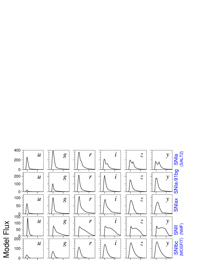
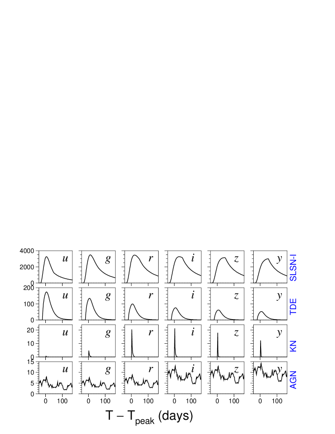
Figure 1.— Each row shows model light curves in the $ugrizy$ passbands for the extragalactic models (Table 1) shown on the right. The time reference $T_{\rm peak}$ corresponds to the peak bolometric flux. For each model, the vertical flux axis is the same for each passband; the flux axis is different for each model. The transient model fluxes are computed for redshift $z=0.02$ ($\mu=34.70$) and AB zero point of 22; thus for ${\rm Flux}=100$, the AB magnitude is $m=22-2.5\log_{10}(100)=17$. For the AGN model (bottom), $z=0.12$ and a random 200 day time-window is shown.

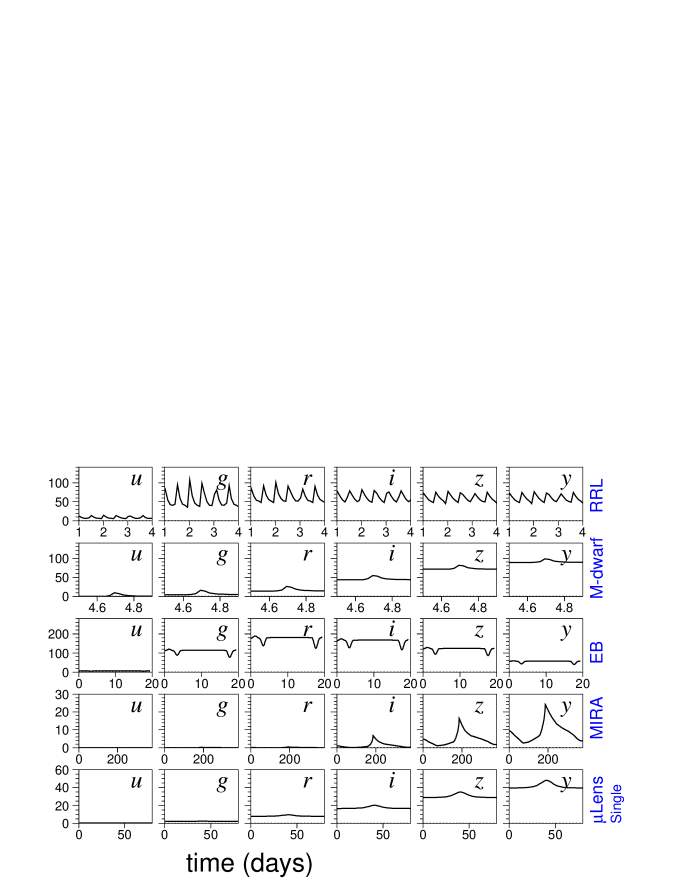
Figure 2.— Each row shows model light curves in the $ugrizy$ passbands for the Galactic models (Table 1) shown on the right. The time axis is different for each model. For each model, the vertical flux axis is the same for each passband; the flux axis is different for each model. The flux zero point is given in Fig. 1 caption.

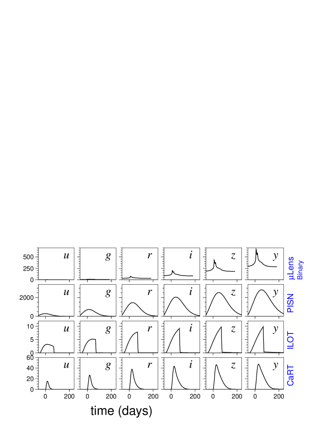
Figure 3.— For models not included in the training set (class ${>}990$ in Table 1), each row shows light curves in the $ugrizy$ passbands for the model shown on the right. For each model, the vertical flux axis is the same for each passband; the flux axis is different for each model. For transient models (lower 3), the redshift, distance, and flux zero point are given in Fig. 1 caption.

There are a total of 14 models in the training set, and $18$ models in the test set. A 19th model ($\mu$Lens-String) was simulated, but was not included in the test set because it brightens for no more than a few minutes and it never satisfies the 2-detection trigger requirement (§6.3).

Table 1 Summary of transient and variable models for .

Model Class	Model		$N_{\rm event}$	$N_{\rm event}$	$N_{\rm event}$	Redshift
Num: Name	Description	Contributor(s)	Gen	Train	Test	Range
90: SNIa	WD detonation, Type Ia SN	RK	16,353,270	2,313	1,659,831	$<1.6$
67: SNIa-91bg	Peculiar type Ia: 91bg	SG,LG	1,329,510	208	40,193	$<0.9$
52: SNIax	Peculiar SNIax	SJ,MD	8,660,920	183	63,664	$<1.3$
42: SNII	Core collapse, Type II SN	SG,LG:RK,JRP:VAV	59,198,660	1,193	1,000,150	$<2.0$
62: SNIbc	Core collapse, Type Ibc SN	VAV:RK,JRP	22,599,840	484	175,094	$<1.3$
95: SLSN-I	Super-lum. SN (magnetar)	VAV	90,640	175	35,782	$<3.4$
15: TDE	Tidal disruption event	VAV	58,550	495	13,555	$<2.6$
64: KN	Kilonova (NS-NS merger)	DK,GN	43,150	100	131	$<0.3$
88: AGN	Active galactic nuclei	SD	175,500	370	101,424	$<3.4$
92: RRL	RR Lyrae	SD	200,200	239	197,155	0
65: M-dwarf	M-dwarf stellar flare	SD	800,800	981	93,494	0
16: EB	Eclipsing binary stars	AP	220,200	924	96,572	0
53: Mira	Pulsating variable stars	RH	1,490	30	1,453	0
6: $\mu$Lens-Single	$\mu$-lens from single lens	RD,AA:EB,GN	2,820	151	1,303	0
991: $\mu$Lens-Binary	$\mu$-lens from binary lens	RD,AA	1,010	0	533	0
992: ILOT	Intermed. Lum. Optical Trans.	VAV	4,521,970	0	1,702	$<0.4$
993: CaRT	Calcium-rich Transient	VAV	2,834,500	0	9,680	$<0.9$
994: PISN	Pair-instability SN	VAV	5,650	0	1,172	$<1.9$
995: $\mu$Lens-String	$\mu$-lens from cosmic strings	DC	30,020	0	0	0
TOTAL	Sum of all models		117,128,700	7,846	3,492,888	—

In addition to modeling light curves, we also modeled the rates. For extragalactic models, our goal was to model physically motivated volumetric rates vs. redshift, $R_{V}(z)$, to generate realistic sample sizes. We achieved this goal for all but the AGN model. For Galactic models we did not receive rate models, and realistic rates would likely have resulted in a data sample too large for a public challenge. We therefore selected arbitrary rates so that Galactic models would comprise ${\sim}10$% of the  sample.

3.1. Extragalactic Models

Most of the extragalactic models are exploding stars called supernovae (‘SN’ in the name), and the peak brightness varies by almost 2 orders of magnitude. The kilonova (KN) model is an explosive event from two colliding neutron stars, and thought to be a primary source of elements heavier than iron. The remaining two extragalactic models are based on interactions with a SMBH at the center of a galaxy: tidal disruption events (TDE) from stars being shredded due to their proximity to a SMBH, and active galactic nuclei (AGN) driven by gas falling into a SMBH.

Fig. 1 illustrates some model features, but beware that there can be significant feature variations within each model class. The SNIa models (SNIa, SNIa-91bg, SNIax) are brightest in the $g$ and $r$ bands, while SNII is brightest in the $u$-band, but only for a short time. SNIbc is faint in the bluer bands ($u,g$), and SLSN-I is bright in all bands, about an order of magnitude brighter than the other SNe. TDE are brightest in the blue bands, and KN are very short-lived. AGN is the only recurring extragalactic model, and can show activity over arbitrary time scales.

Each extragalactic model is defined as a spectral energy distribution (SED) at discrete rest-frame time intervals, and as a function of several parameters characterizing the model. The volumetric rate (per year per cubic Mpc) is described as an analytical function of redshift ($R_{V}(z)$), and is based on measurements, theory, or a combination of both. A summary of rate models is given in Table 2. For rates proportional to star formation with a $z$-dependence from Madau & Dickinson (2014, hereafter MD14), $R_{V}(0)$ is specified in §4. The other rate models include $R_{V}(0)$. Extragalactic events are assumed to be isotropically distributed over the sky, and therefore the DDF and WFD sky area, combined with $R_{V}(z)$, are used to determine the number of generated events.

Table 2 Summary of Extragalactic Rate Models for .

Model
Name	$R(0)$	$R(1)/R(0)\tablenotemark{b}$	$z$-dependence
SNIa	25	2.8	D08 and H18
SNIa-91bg	3	2.8	D08
SNIax	6	5.6	MD14
SNII	45	4.9	S15
SNIbc	19	4.9	S15
SLSN-I	0.02	5.6	MD14
TDE	1	0.15	K16
KN	6	1.0	flat
ILOT	3.9	4.9	S15
CaRT	2.3	5.6	MD14
PISN	0.002	5.4	Pan et al. (2012)

We do not provide rate uncertainties because they are not explicitly used in the simulation. For each model, however, we provide an estimate for the number of observed events used to construct the model, and thus statistical rate uncertainty can be estimated. For science applications, note that there is an implicit uncertainty on the number of simulated events: $\sigma_{N}/N=\sigma_{R_{V}}/R_{V}$.

Next we illustrate some global properties of extragalactic models. Fig. 4 shows the rest-frame luminosity function in the $g$ and $z$ bands; note that SNIa are bright and have a narrow magnitude distribution, making them excellent standard candles for measuring cosmic distances. The brightest models are superluminous supernova (SLSN-I) and pair-instability supernova (PISN), both exceeding $-22$ mag. Fig. 5 shows peak magnitude ($i$-band) vs. FWHM width of the light curve. The duration varies from a few days (KN) to ${\sim}$year (SLSN-I,PISN). There is significant interest in searching unpopulated regions of the mag-versus-width plane.

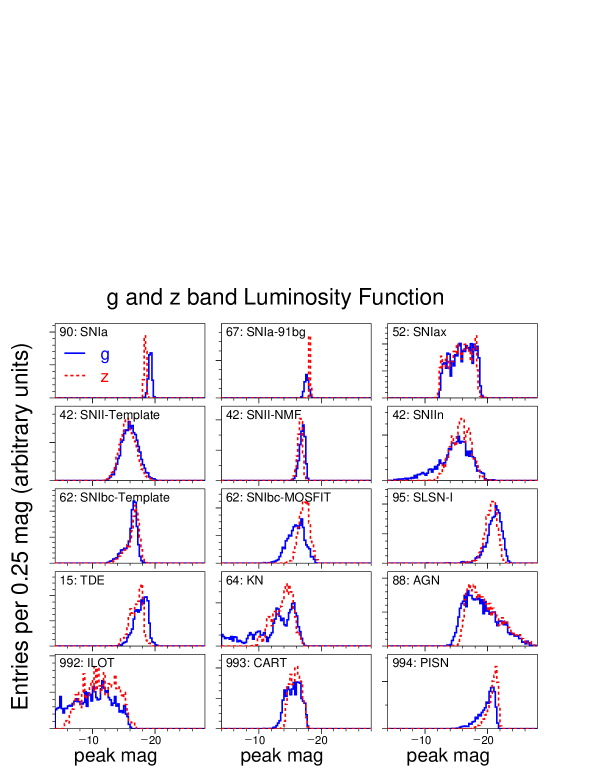
Figure 4.— Peak $g$ and $z$ band magnitude distributions in rest-frame (luminosity function) for extragalactic models. Each panel shows a different set of 4000 model light curves. Models appearing twice show independent implementations.

Fig. 6 shows the redshift distribution for generated events using the rate model, and for the subset satisfying the 2-detection trigger (§6.3) and included in the challenge (red shade). Each distribution depends on the rate model and the luminosity function in each passband. An apparent paradox is the significant difference between the SLSN-I and PISN redshift distributions (after trigger), even though they both have similar peak brightness in the rest-frame (see SLSN-I in Fig. 1, and PISN in Fig. 3). While the SLSN-I model is bright in all LSST passbands, the PISN model is bright only in the redder bands, and thus at high redshift the brightest wavelength region is outside the wavelength sensitivity of LSST.

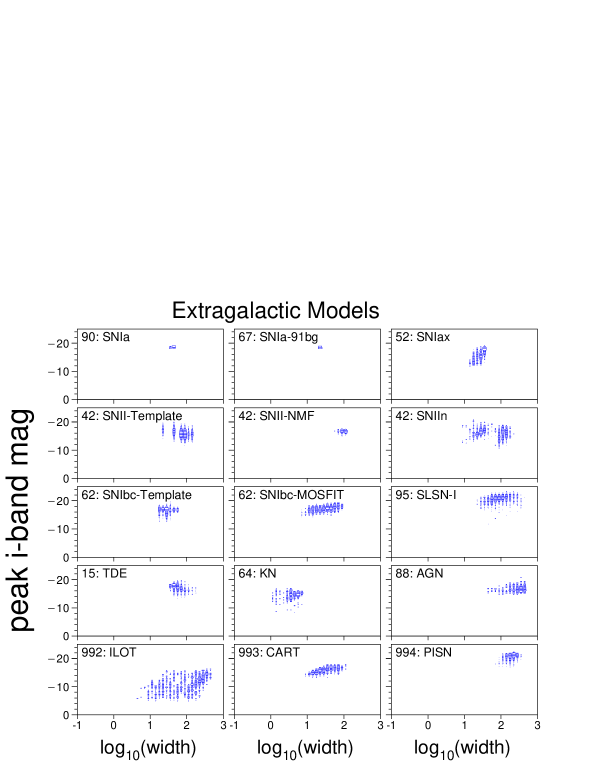
Figure 5.— For extragalacticmodels, two-dimensional histograms of peak $i$-band magnitude (rest-frame) vs. $\log_{10}({\rm width})$, where width is the FWHM (days), or time duration where the flux is greater than half the peak flux. Each panel shows a different set of 4000 model light curves. Models appearing twice show independent implementations. Within each panel, the box sizes are proportional to number of events in the two-dimensional bin.

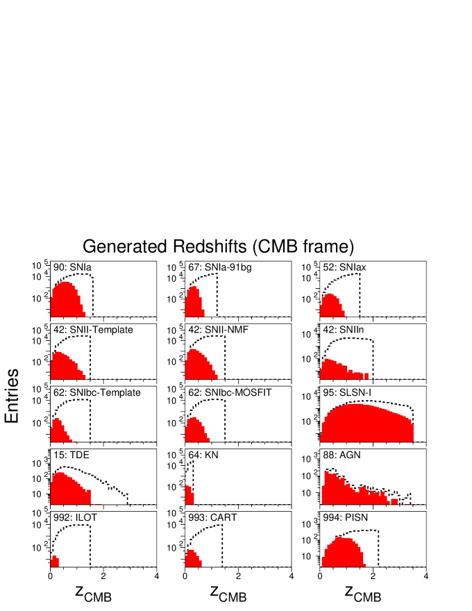
Figure 6.— For extragalactic models, CMB-frame redshifts for all generated events (dashed histogram) and for events passing 2-detection trigger (red shaded). Each panel shows a different model; models appearing twice show independent implementations.

3.2. Galactic Models

Three of the Galactic models in Fig. 2 are recurring (RRL, EB, Mira), with time time scales of $\sim$day (RRL) to a year (Mira). The two nonrecurring models are M-dwarf flares, with time scales less than a day, and $\mu$Lens-Single with time scales from days to years. In addition to recurring and nonrecurring subclasses, there are two distinct mechanisms of variability. The first mechanism is intrinsic, where the stellar brightness varies without interacting with other objects: these intrinsically variable models are RRL, Mira, and M-dwarf. The second mechanism involves an effect between two objects: eclipsing binary (EB) from a pair of stars blocking each other’s light, and microlensing ($\mu$Lens-Single) from a background star that is magnified by a foreground star.

For Galactic models there is no need to store the SEDs, and they are instead defined as a 4-year time sequence of true magnitudes in the $ugrizy$ filter bands. The rate model has two components. The first component is the dependence on Galactic latitude, $b$. For all Galactic models except M-dwarf, we use the profile in Fig. 7a which is based on a fit to stellar data from the Gaia data release 2 (Gaia Collaboration et al., 2018). Fig. 7b shows a smoother profile used for the M-dwarf model. We do not account for Galactic structures such as the Large Magellanic Cloud. The second rate component is the absolute number of generated events, but since we did not obtain Galactic rate models (except for Mira), arbitrary rate values were used. The Galactic rates described in §4 are cited for WFD; the number generated in DDF is 0.083% of the WFD number, where this DDF/WFD ratio was determined from the profile in Fig. 7a.

Figure 7.— $dN/d\cos(b)$ profiles used for Galactic models: (a) based on Gaia data, and (b) smoother profile for M-dwarf model.

A flat distribution corresponds to isotropy.

3.3. Unknown Models

For models not included in the training set (Fig. 3 and class ${>}990$ in Table 1), one is a Galactic model where a background star is lensed by a binary star system ($\mu$Lens-Binary). The remaining three models are extragalactic  supernova explosions. ILOT and CaRT have been observed with low statistics. PISN events have never been observed, and they are predicted to be extremely bright, red, and rare; a high-redshift survey enables the best prospects for discovery.

4. Models-I: Transients and Variables

The subsections below describe each model as follows. First, we give a general overview describing the physical mechanism of the process (e.g., thermonuclear explosion for SNIa), and spectroscopic features which are typically used to classify these objects for training sets. Next, we give implementation details geared for experts, with specific references to methods, data samples, and software packages. Finally, the rate model is given: volumetric rate vs. redshift for extragalactic models, and Galactic latitude dependence for Galactic models. As described in the subsections below, some of the extragalactic models are based on publicly available data from the Sloan Digital Sky Survey (Sako et al., 2018, hereafter SDSS), the Carnegie Supernova Project (Krisciunas et al., 2017, hereafter CSP), and the Supernova Legacy Survey (González-Gaitán et al., 2015, hereafter SNLS).

Ideally, each model would be characterized by observations that have been corrected for survey selection effects in order to model the true underlying populations. However, only the SNIa model accounts for survey selection, and thus the other model populations are less accurate. In addition, several models are based on very low statistics (e.g., 1 observed kilonova event), and thus the true diversity is not fully realized in .

4.1. Type Ia Supernova (SNIa)

4.1.1 Overview of SNIa

A SNIa event is thought to be the thermonuclear explosion of a carbon-oxygen white dwarf (WD) star, the dense exposed core of a former low-mass star. WDs are typically stable, supported by electron degeneracy pressure, but can explode under certain conditions when they are in binary systems. Leading models for the progenitor systems of SNIa (Maoz et al., 2014) include (1) a WD plus a main-sequence or giant companion star, from which the WD accretes material, or (2) the merger of two WDs in a close binary system. In addition to the nature of the companion star in the first progenitor model, other aspects of this process remain uncertain, including the composition of the accreted material, the mass at which the WD explodes (expected to be near the Chandrasekhar limit of 1.4 $M_{\sun}$), and the explosion mechanism (Woosley & Weaver, 1986; Livne & Arnett, 1995; Plewa et al., 2004; Shen et al., 2018).

The thermonuclear fusion of carbon and oxygen results in the formation of iron-group elements (like iron, cobalt, and nickel) and intermediate-mass elements (like magnesium, silicon, sulfur, and calcium). This fusion releases a tremendous amount of energy, ${\sim}10^{51}$ erg in a few seconds, blowing apart the entire WD.

The explosion energy goes into the kinetic energy of the explosion debris (called the ejecta), which flies away at tremendous speeds ($\sim$10,000 km/s) and rapidly cools. Such rapidly cooling debris would not emit much light, except for the fact that some of the newly created elements are radioactive. The radioactive decay of the isotopes ⁵⁶Ni (half-life of 6.1 days) and ⁵⁶Co (half-life of 77 days) deposits energy into the ejecta over a longer time scale. Shortly after the explosion when the material is very dense, this heat energy cannot quickly diffuse out and thus remains trapped until the ejecta expands and rarefies. This heat-trapping leads to visible light emission that rises to a peak luminosity approximately three weeks after the explosion and fades thereafter over the next few months. The SNIa peak luminosity is about 10 billion times brighter than our Sun, and therefore using optical telescopes these events can be viewed from billions of light years away.

The type I classification refers to spectra which have no hydrogen lines. The type Ia classification is associated with the presence of silicon, and in particular, the strong Si II $\lambda$6355 absorption feature. For high-redshift SNIa where the Si II feature is too red for typical spectrographs, there are several bluer features (Ca II, Fe II, Fe III) that are commonly used for identification.

SNIa are probably most well known as “standardizable” candles used to study the expansion history of the universe. Observationally we find that each event has a similar luminosity, and small variations in luminosity are correlated with other observable properties such as the timescale of the light curve (Rust, 1974; Phillips, 1993) and the color of the supernova (Riess et al., 1996; Tripp, 1998). Using SNIa to probe cosmic distances, accelerating cosmic expansion was discovered 20 years ago by Riess et al. (1998) and Perlmutter et al. (1999).

4.1.2 Technical Details for SNIa

We used the SALT-II light-curve model from Guy et al. (2010), and the training parameters determined from nearly 500 well-measured light curves in the “Joint Lightcurve Analysis” (JLA; Betoule et al. 2014). These training parameters describe a time-dependent SED, the SED-dependence on light-curve width, and a color law. The SED model is extended into the ultraviolet (UV) and near infrared (NIR) as described in Pierel et al. (2018), and we use the extended wavelength model from WFIRST simulations (Hounsell et al., 2018). We extrapolated the SED model beyond rest-frame phase $+50$ days using exponential fits to the late-time flux data of SN 2003hv (Leloudas et al., 2009) and SN 2012fr (Contreras et al., 2018).

Each rest-frame SED model depends on a randomly chosen color ($c$) and stretch ($x_{1}$) from the populations in Scolnic & Kessler (2016). The amplitude parameter ($x_{0}$) is computed from $c$, $x_{1}$, and the distance modulus. Intrinsic scatter is implemented with the “G10” SED variation model described in Kessler et al. (2013).

Rate Model:

The volumetric rate versus redshift, $R(z)$, is based on measurements:

$$R(z) = 2.5\times 10^{-5}(1+z)^{1.5}~{}{{\rm yr}^{-1}{\rm Mpc}^{-3}}~{}~{}(z<1)$$ (1)

$$R(z) = 9.7\times 10^{-5}(1+z)^{-0.5}~{}{{\rm yr}^{-1}{\rm Mpc}^{-3}}~{}~{}(z>1)~{}.$$ (2)

For redshifts $z<1$, the rate is from Dilday et al. (2008). For $z>1$ we follow Hounsell et al. (2018). The anonymous journal reviewer noticed a mistake: $R(z=1)$ has a 3% discontinuity.

4.2. Peculiar SNIa subtype (SNIa-91bg)

4.2.1 Overview of SNIa-91bg

The faintest end of the thermonuclear SNIa population is composed of SN1991bg-like objects (e.g. Filippenko et al., 1992). This subgroup is characterized by the following properties: (1) under-luminous, with rest-frame $B$ band magnitude $m_{B}\gtrsim-18$, (2) somewhat red with $B-V\gtrsim 0.3$, (3) fast lived with light-curve width less than 70% of the average SNIa width, (4) lack of a secondary maximum in the infrared bands, (5) light-curve width does not correlate with peak magnitude (Phillips, 1993), and (6) Ti II lines in their spectra.

This subclass comprises 15-20% of the SNIa class (Li et al., 2011; Graur et al., 2017), and they occur mostly in old environments (e.g. González-Gaitán et al., 2011). Although highly debated, recent theoretical studies suggest that their explosion mechanism is the prolongation of normal SNIa with less ⁵⁶Ni powering the light-curve, and lower temperature that leads to an earlier recombination of ionized elements (Hoeflich et al., 2017; Shen et al., 2018; Polin et al., 2019). In contrast to normal SNIa, SNIa-91bg do not follow the stretch-brightness relation (Phillips, 1993) and are therefore not typically used to measure cosmological distances.

4.2.2 Technical Details for SNIa-91bg

To model 91bg-like type Ia supernovae, we start with the SED template series based on Nugent et al. (2002). The near-UV regions are extended using synthetic spectra from Hachinger et al. (2009), which are warped to match light-curves of four subluminous SNe Ia (SN2005ke, SN2006mr, SN2007on, SN2010cr) measured with Swift (Brown et al., 2009). This extended SED template series is used with the SiFTO  light curve fitting model (Conley et al., 2008), which provides best-fit parameters for stretch ($s_{\rm 91bg}$) and color ($\mathcal{C}_{\rm 91bg}$). We fit a sample of spectroscopically-confirmed 91bg-like objects at low redshift from González-Gaitán et al. (2014).

These fitted parameters are used to determine the ranges for stretch (7 bins, $0.65\leq s_{\rm 91bg}\leq 1.25$) and color (5 bins, $0\leq\mathcal{C}_{\rm 91bg}\leq 1$), resulting in a set of 35 SED template series. Each SED template series spans 1000-12000 Å  (10 Å bins), and $-13$ to $+100$ days (1 day bins). The stretch and color are drawn from Gaussian distributions with means of $0.975$ and $0.557$, respectively, and $\sigma$ values of 0.096 and 0.175, respectively. $s_{\rm 91bg}$ and $\mathcal{C}_{\rm 91bg}$ are generated with a reduced correlation of $-0.656$.

While preparing this manuscript we noticed a modeling mistake. Only a single stretch value was used instead of a continuous range, and therefore the variation among the 35 SEDs corresponds to only 5 SEDs. This mistake does not result in leakage, but would result in data-simulation discrepancies if real data were available.

Rate Model: Since SNIa-91bg are found in more passive (and massive) galaxies compared with SNIa (§5.3 of González-Gaitán et al. 2011), we expect the SNIa-91bg rate to have a smaller dependence on the host-galaxy star formation rate. For simplicity, however, we model the SNIa-91bg volumetric rate to be 12% of the SNIa rate:

$$R(z)=3\times 10^{-6}(1+z)^{1.5}~{}{\rm yr}^{-1}{\rm Mpc}^{-3}\$$ (3)

4.3. Peculiar SN (SNIax)

4.3.1 Overview of SNIax

Transient surveys have uncovered a wide range of diversity in supernovae, and LSST will continue this revolution, discovering many thousands of “peculiar” exploding stars. Objects that had been spectroscopic outliers to known classes will become distinct classes. With this in mind we chose to broaden the range of supernovae in  with the aim of photometrically identifying peculiar objects, and also to examine how much confusion they cause for identifying the “standard” supernova types (e.g., SN Ia, Ib/c, II).

The largest class of peculiar white dwarf (thermonuclear) supernovae are Type Iax supernovae, denoted “SNIax” (Foley et al., 2013; Jha, 2017), which are based on the prototype SN 2002cx (Li et al., 2003). SNIax show some similarities to normal SNIa, but in general SNIax have lower luminosity, lower ejecta velocity (measured from spectra), and more variation in these parameters and in their overall photometric behavior compared to normal SNIa. The brightest SNIax could be a contaminant in SNIa samples used to measure cosmological parameters.

4.3.2 Technical Details for SNIax

To generate light curves that mimic the diverse class of SNIax, we began with an SED time-series model generated from spectroscopic and photometric observations of a single well-measured event: SN 2005hk. We used the Open Supernova Catalog (Guillochon et al., 2017, OSC) to collect from various sources near-UV to near-IR photometry (Stanishev et al., 2007; Holtzman et al., 2008; Sahu et al., 2008; Brown et al., 2014; Friedman et al., 2015; Sako et al., 2018; Krisciunas et al., 2017) and optical spectroscopy (Chornock et al., 2006; Phillips et al., 2007; Matheson et al., 2008; Silverman et al., 2012; Blondin et al., 2012).

Three spectra of SN 2011ay (Foley et al., 2013) were added to the collection to fill the phase gap of SN 2005hk spectra between 0 and 10 days after the time of peak brightness. All spectra were warped so that synthetic photometry matches the observed photometry, and the warped SEDs are interpolated in phase and wavelength space to create the full SED time series. Our SN 2005hk SED model is publicly available.

We inferred a luminosity function for SNIax based on the observed sample of $\sim 50$ events presented in Table 1 of Jha (2017). There are strong selection effects for these objects as they span a wide range of absolute magnitude, but we find that a linear luminosity function between $-18\leq M_{V}\leq-13$ with Gaussian roll-offs ($\sigma=$ 0.5 and 0.4 mag at the bright and faint ends, respectively) is adequate to match the observed distribution for a limiting apparent discovery magnitude of $m_{V}=20.3$.

Given an absolute magnitude ($M_{V}$), we estimate a rise time ($t_{\rm rise}$) and decline rate ($\Delta m_{15}$) in the $B$ and $R$ bands using correlations based on Stritzinger et al. (2015) and Magee et al. (2016), as shown in Fig. 2 of Jha (2017). We define distributions for each of four light-curve parameters ($M_{V}$, $t_{\rm rise}$, $\Delta m_{15}(B)$, $\Delta m_{15}(R)$) that capture their correlations and observed scatter. To create a SNIax SED time series, we draw a random sample from these light-curve parameter distributions and “warp” our SN 2005hk SED so that the photometric light curve properties correspond to the four selected parameters. The code for this process is publicly available.

Rate Model: The volumetric SNIax rate was set to $6{\times}10^{-6}\ {\rm yr}^{-1}{\rm Mpc}^{-3}$ at $z=0$ (Foley et al., 2013; Miller et al., 2017), corresponding to 24% of the normal SNIa rate. The redshift evolution of the SNIax rate was chosen to follow the star-formation rate (Madau & Dickinson, 2014) because SNIax environments and host galaxies suggest a young progenitor population (Foley et al., 2009; Valenti et al., 2009; Perets et al., 2010; Lyman et al., 2013, 2018). For event generation, each of the 1,001 SED time series was given equal weight.

4.4. Type II Supernova (SNII)

4.4.1 Overview of SNII

Type II supernovae (SNII) are explosions of massive stars typically with main-sequence masses in the range $8\lesssim M\lesssim 18~{}M_{\sun}$ (Smartt et al., 2009). The explosion results when the core of the star has fused to form the element iron, from which no further nuclear energy can be extracted. The cessation of fusion energy release in the stellar core removes the thermal pressure required to support the star against its own gravity. Without this pressure, the core rapidly (in milliseconds) collapses in a “core collapse” (CC) event, to form either a neutron star or a black hole. Most of the gravitational energy released in the CC goes into enormous emission of neutrinos that mostly escape into space; this neutrino burst was observed more than 30 years ago when about a dozen CC neutrinos were detected from SN 1987A (Hirata et al., 1987). The surrounding material of the star rebounds off the inner core, and a small fraction (${\sim}$1%) of the gravitational energy released in the CC is transferred to this surrounding material, causing it to unbind from the core and be expelled into space. Some of this kinetic energy is thermalized as heat causing the supernova to shine. The optical brightness of CC supernovae can be significantly fainter than SNIa, even though the total energy release is about one hundred times more.

If the dying star has retained a significant amount of hydrogen in its outer layer at the time of explosion, that hydrogen can be seen in the spectrum and we classify this as a SNII. The amount of hydrogen and the density structure of the outer layers affects the supernova light curve in a continuous range from long-lasting brightness plateaus (type IIP) to more linearly declining (type IIL) light curves. Type IIn supernovae are a subtype ($<10$%) that have narrow lines of hydrogen emission in spectra, implying dense pre-existing circumstellar material (CSM) prior to the explosion. These IIn events are thought to be powered by the interaction of hydrogen-rich CSM surrounding the star and the supernova ejecta, converting more of the kinetic energy of the explosion debris into light.

Since SNII are much more abundant than SNIa, (§4.1), there are efforts to standardize the SNII brightness and use them to measure cosmic distances to redshifts $z{\sim}0.5$ (Hamuy & Pinto, 2002; de Jaeger et al., 2015).

4.4.2 Technical Details for SNII

This class includes type II SNe and corresponds to 70% of the CC rate, while the SNIbc class (§4.5) accounts for the remaining 30%. SNII are generated and combined from three distinct models: two models of type II SNe with equal rate, and a 3rd IIn model with a much smaller rate. Approximately 100 well-measured light curves were used to develop these models, and each of these models is described below.

SNII-Templates: We use a time series of SEDs that has been warped such that synthetic photometry matches observed light curves from SDSS and CSP. Each warped SED time series is called a template, and the original templates are from a decade-old classification challenge (Kessler et al., 2010). For , the warping beyond 8000 Å has been updated as described in Pierel et al. (2018). There are 20 templates after discarding those resulting in artifacts in the $z$ and $Y$ band light curves. To match the mean and rms peak brightness in Li et al. (2011), a magnitude offset (1.5 mag) and Gaussian scatter (1.05 mag) are applied.

SNII-NMF: We include a newer model of SNII with an empirical SED that is a linear combination of three ‘eigenvector’ components. To build the model we apply a dimensionality reduction technique known as Non-negative matrix factorization (NMF) to a large sample of SNII multi-band light-curves. This sample includes events used to search for progenitors (Anderson et al., 2014), a compilation of several surveys (Galbany et al., 2016), the SDSS (Sako et al., 2018) and the SNLS (González-Gaitán et al., 2015). The NMF input is a large matrix of observed photometry (SN $\times$ fluxes) and the three resulting light-curve eigenvectors that represent the data are always positive (as opposed to Principal Component Analysis, where eigenvectors may be negative).

Next, we take a large sample of SNII spectra and calculate a single weighted-average SNII spectral time series. These spectra are warped so that their synthetic photometry matches each of the three multi-band light-curve eigenvectors obtained previously. The output of this procedure is a three-component SED basis from which any given SED time series, $S(\lambda,t)$, can be obtained as

$$S(\lambda,t)=a_{1}S_{1}(\lambda,t)+a_{2}S_{2}(\lambda,t)+a_{3}S_{3}(\lambda,t)$$ (4)

where $S_{1,2,3}(\lambda,t)$ are the three warped SED eigenvectors and $a_{1,2,3}$ are the projections, i.e. the factors that multiply the eigenvectors for each SN. The empirical ranges of projections for these eigenvectors are $0.0<a_{1}<0.5$ in 0.1 steps, $0.0<a_{2}<0.07$ in 0.01 steps and $0.0<a_{3}<0.07$ in 0.01 steps. The number of templates in this 3D space is $6{\times}8{\times}8=384$. For each simulated SNII event, $a_{1,2,3}$ are drawn from correlated Gaussian distributions measured from the data: $\sigma_{1,2,3}=0.0854,0.020,0.025$, and reduced correlations $\rho_{1,2,3}=0.241,0.052,-0.74$. Since the $a_{1,2,3}$ values are randomly selected from a continuous distribution, linear 3D interpolation is used to ensure a continuous distribution of SEDs.

While the SNII-Templates include magnitude scatter to match observations, the SNII-NMF scatter was not checked prior to the challenge. This mistake resulted in a luminosity function that is too narrow (Fig. 4).

SNIIn-MOSFiT: We use the MOSFiT software package (Appendix A) to simulate the csm model using the parameter range described in Villar et al. (2017) for Type IIn SNe. In this model, the transient is powered by the forward and reverse shocks which convert their kinetic energy into radiation (Wanderman & Piran, 2015). A number of parameters affect the SEDs, including the CSM density, the CSM mass, the ejecta mass and the ejecta velocity. We assume that the photosphere is stationary and within the CSM. We generate a set of 839 SED time series by sampling physical parameters as described in Villar et al. (2017). We use rejection sampling to match the luminosity function found in Richardson et al. (2014), and require rest-frame $M_{r}<-10$ mag. The faint tail in the $g$-band luminosity function (Fig. 4) is an artifact of the model.

Rate Model: The total CC volumetric rate versus redshift is given by Fig. 6 (green line) in Strolger et al. (2015). The Type II fraction of the total CC rate is 70% (Smartt et al., 2009), and is consistent with the 75% estimate in Li et al. (2011). The rate is split equally among the 20 SNII-Template SED time series, and the SNII-NMF model. The IIn fraction is 6%, and equal weight was given to each of the 839 SED time series.

4.5. Stripped Envelope Core Collapse Supernova (SNIbc)

4.5.1 Overview of SNIbc

Supernovae types Ib and Ic, also known as ‘stripped envelope SNe,’ are a distinct class of core collapse SNe characterized by spectra which lack hydrogen features, and the Ic subclass spectra lack helium. These spectral characteristics imply a progenitor star that has been stripped of its hydrogen and helium envelope before the explosion. While massive stars are the likely progenitor, there is evidence of binary system progenitors (Eldridge & Maund, 2016; Folatelli et al., 2016; Van Dyk, 2017). This transient is likely powered by the radioactive decay of ⁵⁶Ni formed in the supernova ejecta.

SNIbc photometric light curves are similar to those from SNIa (§4.1), but they are fainter and redder (Galbany et al., 2017). In an effort to use photometrically identified SNe Ia to measure cosmic distances and cosmological parameters (Jones et al., 2017), SNIbc events are an expected source of contamination because the brightest SNIbc events overlap the SNIa luminosity function (Fig. 4), and the SNIbc and SNIa colors are similar.

4.5.2 Technical Details for SNIbc

Type Ibc SNe are generated and combined from two distinct models: templates and MOSFiT parameterization. A few dozen well-measured light curves were used to develop these models, and each of these models is described below.

SNIbc-Templates: This is the same procedure as for SNII-Templates in §4.4.2, except the observed SNII light curves are replaced with SNIbc events. There are 13 SED time-series templates (7 Ib plus 6 Ic) after discarding those resulting in artifacts in the $z$ and $y$ band light curves.

SNIbc-MOSFiT: We use the MOSFiT default model (Appendix A), using the SNIbc parameter ranges and distributions described in Villar et al. (2017). We use rejection sampling to match the luminosity function found in Richardson et al. (2014). For event generation, each of the 699 SED time series was given equal weight.

Rate Model: We are not aware of studies that explicitly measure the SNIbc volumetric rate as a function of redshift, but measurements of the CC rate at high redshift often assume constant Ibc/CC fractions when calculating their detection efficiencies. However, for both single and binary star progenitors, the relative Ibc/CC fraction is expected to decline with metallicity. This effect is observed in low-redshift populations when examining the fraction of hydrogen-poor SNe Ibc as a function of host galaxy mass or metallicity. Graur et al. (2017) find a ratio of hydrogen-poor to hydrogen-rich CC SNe that decreases by a factor of $\sim 3.5$ between $8.8<12+\log(\mathrm{O/H})_{\mathrm{T04}}<9.3$. Since we do not model host galaxies, we do not model a metallicity-dependent rate.

The total CC volumetric rate versus redshift is given by Fig. 6 (green line) in Strolger et al. (2015). The Type Ibc rate is 30% of the total CC rate (Smartt et al., 2009), and is split equally among the two SNIbc submodels (Templates and MOSFiT). To generate events with each submodel, equal weight was given to each of the 13 Template SED time series, and also to each of the 699 MOSFiT SED time series.

4.6. Type I Superluminous Supernova (SLSN-I)

4.6.1 Overview of SLSN-I

SLSN-I events are among the brightest optical transients, with peak absolute brightness $\lesssim-21$ mag. Their spectra are blue and lack hydrogen, and their light curves last several months (Chomiuk et al., 2011; Quimby et al., 2011). They tend to be found in metal-poor dwarf host galaxies (Lunnan et al., 2014; Angus et al., 2016), and a significant fraction are well described by a central engine known as a “magnetar:” a neutron star with a strong magnetic field ($B\gtrsim 10^{13}$ G). These rare transients (${\sim}0.1$% of SNIa rate) are a relatively new discovery (Quimby et al., 2011), largely due to the rise in wide-field surveys. Since these events can be up to 50 times brighter than SNIa (§4.1), there are efforts to standardize their brightness and use them to measure cosmic distances to redshifts $z{\sim}3$ (Scovacricchi et al., 2016).

4.6.2 Technical Details for SLSN-I

Based on a few dozen well-measured light curves, we model the central engine as a newly born magnetar, which transfers rotational energy into the surrounding environment as it spins down from dipole radiation. The magnetar’s strength depends on the initial spin period, the mass of the newly born neutron star, and the magnetic field of the system. Recent work (e.g., Nicholl et al. 2017; Villar et al. 2018) has shown that the magnetar model can largely reproduce the diversity of UV through NIR light curves. However, our model neglects pre-peak bumps seen in a number of events (e.g., Nicholl et al. 2015; Smith et al. 2016; Angus et al. 2019). The power source and basic properties of these bumps is currently unknown.

We use the MOSFiT slsn model (Appendix A), which assumes a magnetar engine and blackbody SED with a linear cutoff for $\lambda<3000$ Å (see Fig. 1 in Nicholl et al. 2017). To generate light curves consistent with current observations, we fit a set of 58 well-observed Type I SLSNe to our magnetar model (Nicholl et al., 2017; Villar et al., 2018). In short, we use the fitted physical parameters (e.g., ejecta mass, velocity, magnetic field, initial magnetar spin period, etc.) to generate a multivariate Gaussian which represents the distribution of physical parameters for the underlying progenitor population. We draw sets of physical parameters from this multivariate Gaussian to produce a set of SLSN-I light curves. The visible kink in the light curve (Fig. 1) is due to a temperature floor in the model. Some of the models result in a peak luminosity fainter than $-21$ mag (Fig. 4), and we mistakenly included these faint events.

During the Kaggle competition, a recent analysis of 21 SLSN-I light curves from DES (Angus et al., 2019) suggests that the magnetar model is not sufficient to describe all of these events. To describe the full SLSN-I population, other models may be needed such as interactions with circumstellar material (e.g., Chevalier & Irwin 2011; Chatzopoulos et al. 2013, 2016).

Rate Model: SLSN-I events are observed to occur at a rate of approximately $10^{-8}$ to $10^{-7}~{}{\rm yr}^{-1}{\rm Mpc}^{-3}$ (Quimby et al., 2013; McCrum et al., 2015; Prajs et al., 2017). Spectroscopically confirmed SLSNe have been discovered as far as redshift $z=1.998$ (Smith et al., 2018), and the evolution of their rate with redshift is consistent with the cosmic star-formation history (Prajs et al., 2017). We therefore model the redshift-dependent rate using the star formation history from Madau & Dickinson (2014), with $R(0)=2{\times}10^{-8}~{}{\rm yr}^{-1}{\rm Mpc}^{-3}$. For event generation, each of the 960 SED time series was given equal weight.

4.7. Tidal Disruption Events (TDE)

4.7.1 Overview of TDE

A TDE occurs when a star passes near a SMBH, and the strong tidal fields tidally disrupt the star. Roughly half of the stellar mass is pulled into the SMBH, and the relativistic speed of the in-falling material powers a transient light curve (Rees, 1988). The observed TDE properties depend on the SMBH mass, the stellar properties, and the local interstellar medium (Mockler et al., 2019). The expected SMBH mass range is $10^{6}$-$10^{7}M_{\sun}$; larger masses have a Schwarzschild radius too large to disrupt a star, and instead would swallow the entire star without leaving a visible signal.

The observed characteristics of a TDE are based on the following theoretical expectations: (1) they have a hot, blue continuum, (2) they occur near the center of galaxies, and (3) some have the predicted $t^{-5/3}$ power law for the bolometric light curve (Evans & Kochanek, 1989). While the light-curve luminosity is expected to peak at UV and X-ray wavelengths, a dusty environment near the black hole can result in absorption of UV photons and re-radiation in the NIR (Jiang et al., 2016).

4.7.2 Technical Details for TDE

We use MOSFiT (Appendix A) to simulate the tde model, which assumes that the luminosity traces the fallback rate of the stellar material onto the black hole. To generate light curves consistent with current observations, we fit a set of 11 well-observed TDEs to our model. We use these fitted physical parameters (e.g., the stellar mass, black hole mass, impact parameters, etc.) to generate a multivariate Gaussian, accounting for observational volume associated with each event. We draw sets of physical parameters from this multivariate Gaussian to produce a set of TDE light curves. With this small sample of observed events, the distribution uncertainties are large.

Rate Model: The volumetric rate at redshift $z=0$ is from van Velzen (2018), and the rate vs. redshift is from Kochanek (2016):

$$R(z)=(1.0{\times}10^{-6})\times 10^{-(5z/6)}~{}{\rm yr}^{-1}{\rm Mpc}^{-3}$$ (5)

For event generation, each of the 745 SED time series was given equal weight.

4.8. Kilonova (KN)

4.8.1 Overview of KN

A Kilonova (KN) event is from the merger of a compact binary system containing at least one neutron star: a black hole and a neutron star (BH-NS), or binary neutron star (BNS) system. The two objects collide at roughly half the speed of light, releasing enormous energy in the ejecta and in gravitational waves (GWs). A neutron star is slightly heavier than the sun, and is packed into a small volume with a radius of ${\sim}10$ km; a tea spoon of this dense neutron material has a mass of 10 million tons.

There has long been evidence that the production of heavy elements (beyond iron) in stars and supernovae is not sufficient to account for the observed abundance. To explain this paradox, the existence of KN events has been predicted for decades (Lattimer & Schramm, 1974) to be the primary origin of heavy elements (e.g., gold, platinum), which are formed from rapid neutron capture (r-process) nucleosynthesis. As the neutron star material is expelled from the merger, the material undergoes the r-process to produce heavy neutron-rich elements. The radioactive decay of these elements heats the material, causing it to shine a thousand times brighter than a nova (hence the term ‘kilo-novae’), yet a KN event is still much fainter than SNIa events. KN events are rare, fade rapidly, and are optically faint, making them difficult to find.

After decades of searching for these elusive KNe, the LIGO-Virgo Collaboration (LVC) discovered a BNS signal from a gravitational wave on 2017 August 17 (Abbott et al., 2017c, d); this landmark event is known as GW170817. Two seconds after the LVC detection, a short gamma-ray burst (GRB) signal from the same sky area was detected in space by the Fermi Gamma-ray Burst Monitor (Abbott et al., 2017b). Later that night (${\sim}11$ hr later), several teams independently discovered the optical counterpart using ground-based telescopes; see Fig. 2 of Abbott et al. (2017d), and Coulter et al. (2017); Valenti et al. (2017); Tanvir et al. (2017); Lipunov et al. (2017); Soares-Santos et al. (2017); Arcavi et al. (2017). Over the next few months, dozens of instruments were used to observe this event over a wide range of wavelengths, from radio to gamma rays.

Since the host galaxy for GW170817 was identified and has a well-measured redshift, the combination of GW distance from LVC and spectroscopic redshift was used to measure the Hubble constant ($H_{0}$) with a precision of ${\sim}$15% (Abbott et al., 2017a). The future prospects are excellent for discovering many more KN events, and using them to precisely measure $H_{0}$ (Chen et al., 2018). This is of particular interest in the cosmology community because current precise measurements of $H_{0}$ using a local ladder (Riess et al., 2016) and cosmic microwave background (Planck Collaboration et al., 2018) differ by ${\sim}8$%, or more than 3 standard deviations. This discrepancy has led to a large amount of speculation about the presence of unknown physics in the early universe, and unknown systematic errors in these experiments (Freedman, 2017).

Other science interests related to KNe include element abundances, the neutron star equation of state, and formation mechanisms for compact binaries. For GW170817, the 2 second time difference between the GW and GRB detection shows that the graviton and photon speed are the same to within 1 part in $10^{-15}$; this constraint results in stringent limits on modified theories of gravity (Baker et al., 2017).

4.8.2 Technical Details for KN

Using a single SED time-series model to describe GW170817, Scolnic et al. (2018a) simulated KN rates in past, present, and future surveys, including LSST. We expect more diversity than this single event, so for  we included the set of SED time-series models of BNS mergers from Kasen et al. (2017). These models depend on three parameters: ejecta mass, ejecta velocity, and lanthanide fraction. Increasing ejecta mass results in brighter events, increasing ejecta velocity results in shorter-lived light curves, and increasing the lanthanide fraction results in redder events. We do not have parameterized distributions for these parameters, and therefore each SED was selected with uniform probability. The rest-frame peak magnitude range is $-17$ to $-9$ ($i$ band), compared with $-15.5$ mag for GW170817.

Rate Model: A volumetric KN rate of $1{\times}10^{-6}{\rm yr}^{-1}{\rm Mpc}^{-3}$ is estimated in Scolnic et al. (2018a) based on a compilation of rates in Abbott et al. (2016). For , we increased this rate by a factor of 6 for two reasons: to provide a sufficient training set (${\sim}100$), and to reduce the Kaggle score change from correctly identifying each KN. Near the end of the Kaggle competition, LVC provided rate estimates in The LIGO Scientific Collaboration & the Virgo Collaboration (2018), where the 90% confidence upper limit for BNS mergers is $3.8{\times}10^{-6}~{}{\rm yr}^{-1}{\rm Mpc}^{-3}$, or roughly 60% of the rate used to simulate . For event generation, each of the 329 SED time series was given equal weight.

4.9. Active Galactic Nuclei (AGN)

4.9.1 Overview of AGN

An Active Galactic Nucleus (AGN) refers to the central region of a galaxy that is much brighter than average, and AGN are among the brightest extragalactic sources. It is hypothesized that AGN activity is a phase in the evolution of most galaxies, and is caused by a large influx of gas onto a SMBH in the center of the galaxy. The gas influx could be from galaxy mergers (Sanders et al., 1988; Barnes & Hernquist, 1991; Hopkins et al., 2006), or recycled stellar material. The associated accretion disk results in the emission of electromagnetic radiation from radio to X-ray wavelengths.

AGN exhibit stochastic, aperiodic variability with ${\sim}10$% variations on timescales of weeks to years. This characteristic variability has been used, along with other features, to identify AGN in previous time-domain surveys.

Here we give a few examples of how AGN are used to study astrophysics. The energy outflows from AGN can heat gas in the interstellar medium, which can reduce or stop star formation; thus AGN feedback is an important component in understanding galaxy evolution (Silk & Rees, 1998). Next, a technique called reverberation mapping (Blandford & McKee, 1982; Shen et al., 2015) has been developed to measure the mass of the central SMBH. The ultimate goal is to measure these masses as a function of redshift and AGN environments, and to learn about black hole formation over cosmic time. Finally, there have been attempts to standardize the AGN brightness (Watson et al., 2011; La Franca et al., 2014; Risaliti & Lusso, 2017) to measure the cosmic expansion history at very high redshifts.

4.9.2 Technical Details for AGN

The LSST Project CatSim framework (Connolly et al., 2010, 2014) provides a simulated volume of galaxies by applying a semi-analytic model of galaxy formation (De Lucia et al., 2006) to the Millennium $N$-body simulation (Springel et al., 2005). This provides us with a population of galaxies on a $4.5\times 4.5$ deg² patch of sky. The entire sky is simulated by tiling this patch over the entire celestial sphere. The semi-analytic model determines which galaxies contain AGN. In its quiescent phase, each AGN is represented by the composite AGN SED derived from SDSS observations in Vanden Berk et al. (2001). As described in MacLeod et al. (2010), SED variability is added in the form of a damped random walk in $\Delta m_{b}$, where $m_{b}$ is the magnitude of the AGN in the requested band $b$.

Each AGN is assigned: (i) a characteristic timescale corresponding to $\tau$ in Eq. 1 of MacLeod et al. (2010), (ii) a unique integer to seed a random number generator, and (iii) six structure function values (one for each LSST band) corresponding to the $\text{SF}_{\infty}$ parameter in Eq. 3 of MacLeod et al. (2010). For each simulated AGN observation, a damped random walk with $\text{SF}_{\infty}=1$ is started well before the start time of the survey, and is propagated forward to the requested observation time. The result of this random walk is multiplied by the structure function of the requested LSST band to determine $\Delta m_{b}$. Note that only a single damped random walk is simulated for each AGN. Any variation in color of the AGN is solely due to the different structure function values assigned to each LSST band, corresponding to different amplitudes in the random walk through $\Delta m_{b}$.

The Python code implementing this model is publicly available.

Rate Model: AGN were generated with an isotropic distribution on the sky. A arbitrary total of 175,500 events were generated. For event generation, each of the 5490 model light curves was given equal weight.

4.10. RR Lyrae (RRL)

4.10.1 Overview of RRL

RRL are periodic variable stars from the horizontal branch that formed more than 10 billion years ago. Their pulsations result in brightness variations on ${\sim}1$ day time scales, and their well known period-luminosity-metallicity (P-L-Z) relation makes them excellent distance indicators (Catelan & Smith, 2015). RRL are also used to probe star clusters, streams, and satellite galaxies within the Milky Way. While RRL are useful probes within the Milky Way, their low luminosity limits their use as extragalactic distance indicators.

4.10.2 Technical Details for RRL

The LSST Project CatSim framework (Connolly et al., 2010, 2014) provides a simulated distribution of Milky Way stars based on color-space distributions drawn from SDSS using the GalFast model of Jurić et al. (2008). RRL variability is added to each star by using color-space matching to assign a template light curve from Sesar et al. (2010). Light curves for  were selected with quiescent $r$-band magnitudes between $16.0<r<26.0$. The model light curves are publicly available.

Rate Model: RRL were generated with the Galactic latitude distribution in Fig. 7a. An arbitrary total of 200,200 events were generated. For event generation, each of the 49,130 model light curves was given equal weight.

4.11. M-dwarf stellar flare (M-dwarf)

4.11.1 Overview of M-dwarf

Stellar flares on cool dwarf stars are anticipated to be a major source of transients in the LSST data stream. Because flaring activity is stochastic, potentially very energetic (Kowalski et al., 2009), and most common on low temperature stars that may not be detected in the quiescent phase (West et al., 2011; Walkowicz et al., 2011), stellar flares are expected to be discovered as transients rather than as extensions of known variable light curves.

Based on detailed observations of well-known flare stars (Hawley et al., 2014) and the analysis of light curves from survey data (Kowalski et al., 2009; Walkowicz et al., 2011), typical flares can range in duration from a few minutes to several tens of minutes, and the amplitude can vary from ${\sim}0.01$-0.1 mag, with some extreme flares producing up to 5 mag in brightness variability.

4.11.2 Technical Details for M-dwarf

We begin with a realistic distribution of cool dwarf stars on the sky, each with a unique light curve representing a stochastic population of stellar flares. This distribution is from the SDSS-based GalFast model (Jurić et al., 2008), as served through the LSST Project’s CatSim framework (Connolly et al., 2010, 2014). We include all simulated stars redder than $r-i=0.62$ as candidate flaring dwarfs.

We simulate individual stellar flares using the empirical model of Davenport et al. (2014), which parameterizes flares in terms of their amplitude and duration. Light curves for individual stars are generated by assigning a realistic random sample of flares along the duration of the simulated light curve. This sample of flares is taken from Hilton (2011) and Hilton et al. (2011), who provide distributions of flare energies for five different classes: (1) early type active, (2) early type inactive, (3) mid type active, (4) mid type inactive, and (5) late type (see Eq. 4.2 and Table 4.3 of Hilton 2011). Here “early” corresponds to spectral types M0-M2, “mid” corresponds to spectral types M3-M5, and “late” corresponds to a star cooler than M5.

For each light curve, we randomly select flare times from a uniform distribution so that the number of flares over the duration of the light curve matches the cumulative rate of flares per hour at the minimum energy reported in Table 4.3 of Hilton (2011). For each flare time, we randomly assign a flare energy according to

$$E=E_{\rm min}\times(1.0-X)^{\left(1.0/\beta\right)}~{},$$ (6)

where $X$ is a random number between 0 and 1, and $E_{\rm min}$ and $\beta$ are set to values in Table 4.3 of Hilton (2011). This prescription assures that the energy distribution of flares matches that given by Table 4.3 and Eq. 4.2 of Hilton (2011). To avoid modeling the poorly sampled energy tail, a flare drawn with an energy exceeding $10^{34}$ erg is clipped to exactly $10^{34}$ erg.

Next, we determine the flare’s amplitude and duration. By studying the distributions of flares on the known flare star GJ 1243, Hawley et al. (2014) provide a relationship between flare energy, duration, and amplitude (see their Figure 10). Assuming these relationships hold for all stellar flares, we take the energy distributions from Hilton (2011) and convert them into flare durations by randomly drawing from Gaussians whose mean and variance as a function of flare energy is heuristically fit to the distribution in the middle panel of Figure 10 from Hawley et al. (2014). We motivate this assumption using Fig. 16 of Chang et al. (2015), which shows no significant evolution in the relationship between flare duration and energy as a function of flare magnitude in the population of flares observed in M37. Once the energy and the duration have been specified, the amplitude is numerically solved by assuming that the flare profile has the shape specified by Davenport et al. (2014). To determine a flare’s colors, we model each flare as a 9000 K blackbody according to Hawley et al. (2003).

To assign spectral types to our simulated stars, we convert Table 2 of West et al. (2011) into a probability density, $P({\rm type},r-i,i-z)$, which depends on spectral type and stellar colors $r-i$ and $i-z$. Each star is assigned to the spectral type such that $P({\rm type},r-i,i-z)$ is maximized. Finally, we assign an “active” or “inactive” status by comparing the star’s position above the simulated galactic plane with Fig. 5 of West et al. (2008), which presents the fraction of stars that are magnetically active as a function of distance above the galactic plane and drawing from the appropriate distribution. Magnetic activity is not necessarily the same as flaring activity (the nomenclature of Hilton et al. 2011; Hilton 2011). We therefore use the bottom panel of Figure 12 of Hilton et al. (2010), which shows both the total distribution of flare active and magnetically active stars as a function of distances from the galactic plane, to derive a ratio between the scale height of flare active and magnetically active stars in the galaxy. We use this ratio to correct the distribution of active stars from West et al. (2008).

The Python code used to generate this model is publicly available.

Rate Model: M-dwarf events were generated with the Galactic latitude distribution in Fig. 7b. An arbitrary total of 800,800 events were generated. For event generation, each of the 1,846 model light curves was given equal weight. While each template light curve was generated more than 400 times, the efficiency is only ${\sim}10$% because of the short light curve duration, and thus the the re-use factor in the data set is ${\sim}50$.

4.12. Eclipsing Binary Stars (EB)

4.12.1 Overview of EB

Eclipsing binary stars (EBs) are systems where the orbital plane is aligned with our line of sight, resulting in eclipses as the stars orbit their common center of mass. These systems are relatively ubiquitous: the census of Kepler targets revealed a $\sim$1–2% occurrence rate across the sky (Prša et al., 2011; Kirk et al., 2016), with the rates increasing towards the galactic plane.

Eclipsing binary light curves are generally easy to recognize. Provided a sufficiently high signal-to-noise ratio, eclipses provide readily distinguishable signatures in light curves: V-shaped or U-shaped flux dips during eclipses, along with the out-of-eclipse variability owing to tidal and rotational distortion of the stars known as ellipsoidal variations. The real power of EBs becomes evident when both components contribute a comparable amount of light; we see both components in the spectra of EBs and we call such systems double-lined spectroscopic binaries or SB2. Coupled with photometric data, SB2 systems provide us with masses and radii of individual components from first principles: Newtonian dynamics and geometry. SB2 systems comprise ${\sim}25$% of all EBs, and the state-of-the-art precision of masses and radii is ${\sim}1$%. EBs are therefore indispensable astrophysical laboratories for measuring stars, and for providing calibration opportunities across stellar and galactic astrophysics (Torres et al., 2010). They also serve as reliable distance gauges within our Galaxy and beyond (Guinan et al., 1998).

4.12.2 Technical Details for EB

We used Galaxia (Sharma et al., 2011), a stellar population model based on the Besançon model of the Galaxy (Robin et al., 2003), to generate a synthetic model of single stars in our Galaxy to the depth of $r=24.5$.

We paired coeval stars into binary systems according to the observed distributions in multiplicity rates, orbital period, mass ratio, and eccentricity (Raghavan et al., 2010; Duchêne & Kraus, 2013; Kirk et al., 2016; Moe & Di Stefano, 2017). Other orbital properties, namely inclination, argument of periastron and semi-major axis, were either computed or drawn from expected theoretical distributions. All other physical properties (temperatures, individual masses and radii, distance, etc.) were inherited from the stellar components drawn from the Galaxia sample. The generated systems were tested for stability and unphysical or unstable systems were removed from the sample. The process is described in more detail in Wells et al. (2017) and M.Wells & A.Prša (2019, in preparation). The light curves were calculated using PHOEBE (Prša et al., 2016), an eclipsing binary modeling suite that supports LSST passbands.

Rate Model: The Galactic latitude dependence is from Fig. 7a. The overall number of generated events was arbitrarily chosen to be 220,000. For event generation, each of the 500 model light curves was given equal weight.

4.13. Pulsating Variables Stars (Mira)

4.13.1 Overview of Mira

Mira-type variables are ${\sim}1M_{\sun}$ stars in the late stages of evolution, which undergo stellar pulsation. These cool red giants with radius typically 200 times that of the sun are also very bright, often with luminosities that are 2000 times brighter than the sun. Mira variables are difficult to model given the complex balance of pulsation, shocks, and radiation pressure in the star.

Named after the most famous example of such a star, $o$Ceti, Mira variables are observed to be either oxygen-rich or carbon-rich. The chemical composition of the star affects its luminosity changes due to material being dredged up from the stellar interior; however the exact fundamental properties of Mira variables, like their mass-loss rate or metallicity, are hard to measure from their spectra. They vary on periods of $P\sim 330$ days, however their maximum brightness varies each cycle and therefore without a clear period-luminosity relationship these stars are not good distance indicators.

4.13.2 Technical Details for Mira

We model Mira variable SEDs through the Cool Opacity-sampling Dynamic EXtended (CODEX) atmospheric model series for M-type (oxygen-rich) Mira variables (Ireland et al., 2008, 2011). The models include self-excited pulsation with specific approximations for convective energy transport (see Keller & Wood, 2006, for details) and employ an opacity sampling method for radiative transfer in local thermodynamic equilibrium. Although these models were originally developed to explain interferometric observations of Mira variables at mid-infrared and radio wavelengths, they are still useful to produce SEDs across the optical wavelengths covered by the LSST passbands.

A large number of reference light curves were constructed from five SED template realizations of the underlying Mira CODEX models for $o$Ceti (‘compact’, ’extended’) and from RCas. These model outputs are available online. These SED fluxes were interpolated between the modeled time intervals. The model time ranges were clipped to ensure that only integer periods of the oscillations were included. For each realization, the pulsation period of the variable was randomly selected from a Gaussian distribution with a mean of $\langle P\rangle=330$ days and $\sigma=0.1\langle P\rangle$.

The light curves were generated by producing synthetic photometry from the model SED using the LSST passbands and the AB system. The distribution of $i$ band magnitudes was chosen to reflect the distribution from the Optical Gravitational Lensing Experiment (OGLE, described below) and the magnitudes in the other bands were determined from relationships in the CODEX-generated SED fluxes.

Rate Model: The Galactic latitude dependence is from Fig. 7a. The overall number of generated events is 1,490, and was computed from OGLE (OGLE, Soszyński et al., 2009) General Catalog of Variable Stars. The full OGLE sample of long-period variables includes 1667 Mira stars along with the photometric and astrometric properties of these stars. We restrict the sample to have declination $\delta<10$ deg, $i$ band magnitude $i>15$, and Galactic extinction $E(B-V)<3$. For event generation, each of the 3,000 model light curves was given equal weight.

4.14. Microlensing from a Single Lens ($\mu$Lens-Single)

4.14.1 Overview of $\mu$Lens-Single

As a special case of gravitational lensing, microlensing occurs when a foreground star (the lens) crosses the line of sight of a more distant star (the source). General relativity predicts that several images of the source are created. These images are separated by a few angular Einstein ring radii $\theta_{E}$:

$$\theta_{E}=\sqrt{{{4GM_{l}}\over{c^{2}}}(D_{l}^{-1}-D_{s}^{-1})}$$ (7)

where $G$ is the gravitational constant, $c$ is the speed of light in vacuum, $M_{l}$ is the mass of the lens, and $D_{l}$ and $D_{s}$ are distances to the lens and source, respectively (Paczynski, 1986). In the case of microlensing, the mass of the lens is small ($\sim$few solar masses) and $\theta_{E}$ is order of milli-arcseconds, leading to indistinguishable images, even with the highest resolution instrument to date. The images are also magnified, creating a brightening of the source. The total magnification factor versus time, defined as $A(t)$, is the fundamental observable predicted by Refsdal (1964). In the simplest case of a single source and a single lens (both point sources), one can derive from general relativity (see for example Paczynski 1986):

$$A(t)={{u(t)^{2}+2}\over{u(t)\sqrt{u(t)^{2}+4}}}$$ (8)

where the impact parameter $u(t)$ is the angular distance of the source from the lens, divided by $\theta_{E}$. The dependence on time ($t$) is due to the relative angular motion ($\mu_{\rm rel}$) between the source and the lens. Often, the impact parameter is described with three fundamental parameters:

$$u(t)^{2}=u_{o}^{2}+{{(t-t_{o})^{2}}\over{t_{E}^{2}}}$$ (9)

where $u_{o}$ is the minimum impact parameter at the time of maximum magnification, $t_{o}$, and $t_{E}=\theta_{E}/\mu_{\rm rel}$ is the Einstein ring crossing time.

The real observable from image analysis is the variation of the total flux on the line of sight:

$$f_{\lambda}(t)=f_{s,\lambda}A(t)+f_{b,\lambda}$$ (10)

where $f_{s,\lambda}$ is the source flux at wavelength $\lambda$, and $f_{b,\lambda}$ is the blend flux along the line of sight not related to the lensing events. The blend flux is often from other stars along the line of sight, particularly for dense fields near the Galactic center, but can also come from the lens itself. If the flux from the lens is measured, the properties of the lens (i.e. the distance and the total mass) are much better constrained from observations (e.g., Beaulieu 2018). A more complete review on microlensing is given in Mao (2012) and Tsapras (2018).

4.14.2 Technical Details for $\mu$Lens-Single

Two independent methods were used to generate $\mu$Lens-Single events: PyLIMA and GenLens. PyLIMA used the Gaia catalog to select source stars, and did not include blending. GenLens used a simulated LSST star catalog to generate a source star, and also selected a second unlensed star. Light from the second star altered the lensing light curve through blending. This GenLens model was also used to model binary lenses as described in §4.15.

PyLIMA: This method is based on the first open-source microlensing software tool (Bachelet et al., 2017). We compute $u(t)$ (Eq. 9) by selecting $t_{o}$ from a uniform distribution spanning 2850 days, $u_{o}$ from a uniform distribution in [0,1], and $t_{E}$ from a log-normal distribution (mean$=3.1$, $\sigma=1.0$) that mimics the observed distribution toward the Galactic Bulge (Mróz et al., 2017). We neglect second order effects, such as distortion induced by the rotation of the Earth around the Sun, known as the microlensing parallax (Gould, 2004).

After computing the magnification $A(t)$ from $u(t)$, the source and blend fluxes are needed. As a simplification, we ignore blending from other stars. To obtain a realistic source star magnitude distribution, we first select a random position in the sky from a uniform distribution in right ascension and declination. Next, we query the Gaia DR2 catalog at this position (Gaia Collaboration et al., 2018) and choose a random star (with $T_{\rm eff}>3500$ K). From the luminosity, we derive the mass of the star using $L\sim M^{3.5}$ and its surface gravity using the radius measurement from Gaia. Using the surface gravity and effective temperature, an artificial spectrum of this star is estimated using the models from Kurucz (1993), and implemented with pysynphot. The spectrum is transformed to AB magnitudes in the six LSST passbands using the speclite module. To avoid saturation in the LSST footprint, the star brightness is reduced by 4 mag.

GenLens: This method uses information from known microlensing events, and selects the source and lens from an LSST catalog with $ugrizy$ magnitudes for almost 17 million simulated stars. The most important characteristic of a microlensing event is the Einstein-radius crossing time, $t_{E}$. For point-lens events, $t_{E}$ is the only quantity that can be derived from model fits to the light curve, which contains information about the mass of the lens. We created a $t_{E}$ distribution from 24,000 microlensing event candidates that had been discovered through the combined efforts of several survey teams (Udalski et al., 1992; Alcock et al., 1993; Bond et al., 2001). These observed events are close to the Galactic bulge, and we make an approximation using these events to populate the entire LSST-WFD area. The estimated $t_{E}$ values range from less than a day to more than 500 days.

After choosing a random $t_{E}$ value from the measured distribution, we select the distance of closest approach, $u_{o}=U_{[0,1]}{\times}R_{E}$, where $U_{[0,1]}$ is a random number drawn from a uniform distribution over $[0,1.67]$, and $R_{E}$ is the Einstein radius. In the absence of blending, $u_{o}$ determines the value of the peak magnification. The maximum value $u_{o}=1.67\,R_{E}$ corresponds to the minimum peak magnification, $A_{\rm peak}=1.1$. Blending is included by adding flux from a second (unmagnified) star randomly chosen from the LSST catalog. Because we start with the value of $t_{E}$, we have a relationship between the duration of each time interval in our simulation and the value of the Einstein-radius crossing time. We therefore do not need to separately generate values of the lens mass or of the velocities of source star and lens. We compute the value of the magnification every 15 minutes, and to limit the output library size, we store magnitudes with changes $>0.001$ mag. The light curve duration for each event was $14\,t_{E}.$

Rate Model: $\mu$Lens-Single events were generated with the Galactic latitude distribution in Fig. 7a. A total of 2,820 events were generated (half for each method). The 19,360 light-curve models were selected with a probability proportional to the light-curve duration.

4.15. Microlensing from Binary Lens ($\mu$Lens-Binary)

4.15.1 Overview of $\mu$Lens-Binary

For $\mu$Lens-Single events (§4.14), light curves rise gradually from baseline, are symmetric, and are described by a simple mathematical function. The majority of observed microlensing light curves have the general appearance expected for the $\mu$Lens-Single model. Simulated $\mu$Lens-Binary light curves, however, exhibit great variety, including asymmetries, multiple peaks, plateaus, and quasiperiodic behavior (Mao & Paczynski, 1991; Mao & Di Stefano, 1995; Guo et al., 2015). Caustic crossing light curves exhibit sharp variations in magnification, and this $\mu$Lens-Binary feature has been commonly observed (Udalski et al., 1994). Other $\mu$Lens-Binary light curves, however, have been found in much smaller numbers than expected (Di Stefano, 2000). For example, only a few light curves show evidence of binary rotation, and the rotation in these cases is modest (Dominik, 1998; Afonso et al., 2000).

4.15.2 Technical Details for $\mu$Lens-Binary

Using the same GenLens method as in §4.14.2, the $\mu$Lens-Binary model accounts for blending effects, and also the orbital motion of the binary system. We start by generating $t_{E}$ using the same distribution as for $\mu$Lens-Single events. We choose the value of $u_{o}$ from a uniform distribution with a maximum value of $2\,R_{E}$. The peak magnification of binaries can be high, even for values of $u_{o}$ as large as $2\,R_{E}.$

Because binary lenses are more complex than point lenses, it is necessary to select additional parameters to describe $\mu$Lens-Binary. First is the relative transverse speed of source and lens in the observer’s frame ($v$), selected from a uniform distribution extending from $15$ km s^-1 to $105$ km s^-1. Second is the distance to the source, $D_{S}$, which is fixed at 8 kpc. Third is the distance to the lens, $D_{L}$, which was selected from a uniform distribution between $10$ pc and $D_{S}$. With $t_{E}$, $v$, $D_{S}$, and $D_{L}$, the total mass of the binary lens system can be determined. To eliminate lensing from objects greatly exceeding the largest known black hole masses, we excluded events with $t_{E}>300$ days if $D_{L}<1$ kpc.

Two properties of the binary system determine the characteristics of the lensing light curve. One is the mass ratio, $q=M_{2}/M_{1}$, where $M_{2}<M_{1}$. To model stellar binaries we select $q$ from a uniform distribution in $[0.2,1.0]$. The second property is $\alpha=a/R_{E}$, where $a$ is the separation between the two binary objects, and $R_{E}$ is the Einstein radius. We select $\alpha$ from a uniform distribution in $[0.2,2.0]$. We also select a random orientation of the orbital plane and random direction of orbital motion (prograde or retrograde with equal probability).

Note that binary systems with small values of $\alpha$, large orbital periods, and nearly edge-on configurations can produce light curves very similar to $\mu$Lens-Single light curves. The most dramatic differences between $\mu$Lens-Single and $\mu$Lens-Binary light curves occur when $a$ is comparable to $R_{E}$, and Fig. 8 illustrates this difference for the same source star.

Rate Model: $\mu$Lens-Binary events were generated with the Galactic latitude distribution in Fig. 7a. An arbitrary total of 1,010 events were generated. The 11,860 light-curve models were selected with a probability proportional to the light-curve duration.

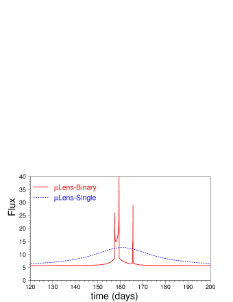
Figure 8.— For a fixed source star, example microlensing light curve ($r$-band) for binary lens (red curve) and single lens (blue dashed curve). The flux-to-mag conversion is given in Fig. 1 caption.

4.16. Intermediate Luminosity Transients (ILOT)

4.16.1 Overview of ILOT

Intermediate Luminosity Transients (ILOTs) have peak optical luminosities between those of supernovae and novae, and display clear signs of interaction between their ejecta and a dense surrounding circumstellar material (CSM). These transients are sometimes associated with the progenitors of Type IIn supernovae.

4.16.2 Technical Details for ILOT

We use the MOSFiT software package to generate the csm model, using the ILOT parameter range from Table 1 in Villar et al. (2017). We model SEDs following Chatzopoulos et al. (2012), and assume that the forward and reverse shocks from the ejecta-CSM interaction convert their kinetic energy into radiation. This model is identical to that used for Type IIn SNe in §4.4.2, however, the explored parameter space (i.e., the ejecta masses and energies) is significantly different, leading to a distinct class of objects. The rapid drop after ${\sim}100$ days (Fig. 3) is an artifact of how MOSFiT models the nebular phase.

Rate Model: For the volumetric rate, we assume the same rate vs. redshift as for Type IIn: 6% of the CC rate from Strolger et al. (2015). For event generation, each of the 385 SED time series was given equal weight.

4.17. Calcium-rich Transients (CaRT)

4.17.1 Overview of CaRT

CaRT events, as their name suggests, appear to be rich in Calcium based on their spectra. These events are a mysterious class with few members. They are somewhat dim compared with more traditional supernovae and occur far from their host galaxies (Lunnan et al., 2017). The rapid light-curve evolution indicates a small ejecta mass (${\lesssim}0.5$ M_⊙).

4.17.2 Technical Details for CaRT

We model CaRT with the MOSFiT default model, powered by the radioactive decay of Nickel. We generate light curves empirically by matching observations from Lunnan et al. (2017) and Milisavljevic et al. (2017), and setting uniform priors in ejecta mass, ejecta velocity, and nickel fraction. Models were kept for $-18<M_{r}<-14$, the approximate luminosity range of observed CaRTs. Since  does not include host galaxies, we do not model the large CaRT distances from their hosts.

Rate Model: Perets et al. (2010) report a relative CaRT rate of $(7\pm 5)$% of the SNIa rate. We simulated a volumetric rate following the star formation rate from Madau & Dickinson (2014), with $R(0)=2.3{\times}10^{-6}~{}{\rm yr}^{-1}{\rm Mpc}^{-3}$, or about 9% of the SNIa rate. For event generation, each of the 225 SED time series was given equal weight. While preparing this manuscript, we learned that a few months before  started, PTF had used a sample of 3 events to report a CaRT rate that is $\times 5$ higher ($2.5\sigma$) than what we used in  (Frohmaier et al., 2018).

4.18. Pair-instability Supernova (PISN)

4.18.1 Overview of PISN

Pair-instability Supernovae (PISN) are thought to arise when low-metallicity Population III stars, with $M_{*}{\sim}140$-$260M_{\odot}$, reach sufficiently high core temperatures that $\gamma$-rays produce electron-positron pairs. This leads to a drop in the internal pressure, resulting in a gravitational collapse which initiates a thermonuclear explosion that obliterates the entire star (Barkat et al., 1967; Kasen et al., 2011). Like some core-collapse supernovae, the optical light curves of PISNe are powered mainly by the radioactivity decay of ⁵⁶Ni; however, PISNe typically have larger ejecta masses, higher kinetic energies, and much brighter luminosities (similar to those of SLSN-I, §4.6).

Observing and identifying PISN light curves is challenging because they are expected to be found at high redshift where the observed light curve can last several years. Evidence for a few PISN events has been reported in Gal-Yam et al. (2009), Cooke et al. (2012), and Kozyreva et al. (2018).

4.18.2 Technical Details for PISN

We use the MOSFiT default model, with the PISN parameter ranges described in Villar et al. (2017).

Rate Model: We use a theoretically motivated function of redshift in Pan et al. (2012) to describe the volumetric rate:

$$R(z) = [1.98+6.38z+6.55z^{2}-4.42z^{3}$$

$$+0.8312z^{4}-0.0508z^{5}]~{}{\rm yr}^{-1}{\rm Gpc}^{-3}\$$

At redshift $z=0$, the PISN rate is ${\sim}10^{4}$ lower than the SNIa rate, and thus PISN detections are expected at higher redshifts. For event generation, each of the 1,000 SED time series was given equal weight.

4.19. Microlensing from Cosmic Strings ($\mu$Lens-String)

4.19.1 Overview of $\mu$Lens-String

Cosmic superstrings are hypothesized to have been formed from the basic constituents of string theory that have been stretched to macroscopic size during the epoch of inflation. For a review of inflation in string theory see Baumann & McAllister (2015), and for a review of superstring properties see Chernoff & Tye (2015). Cosmological evolution of these entities yields a network of long, horizon-crossing segments and sub-horizon loops. For a review of this general scenario see Vilenkin & Shellard (2000). For string tensions that are not ruled out by observations, the loops are the dominant component of interest (Chernoff & Tye, 2018), and are expected to cluster with dark matter when structure forms in the universe (Chernoff, 2009). These loops have a negligible contribution to the galaxy’s total mass, but are potentially detectable as stellar flux variation if a source (star), lens (string) and observer are suitably aligned (Vilenkin, 1981, 1984; Bloomfield & Chernoff, 2014).

A direct search for these fossil superstring remnants of the early universe requires repeated flux measurements of stars (Chernoff & Tye, 2007). String microlensing models predict that the brightness of an unresolved, point-like source (star) is magnified by exactly a factor of 2, which is quite distinct from other microlensing signatures. Microlensing of stellar sources in the galaxy repeats $\sim 10^{3}$ times because the loop center of mass moves at the halo velocity whereas the internal oscillations of the loop are relativistic. These distinctive features (factor of 2 enhancement, repetitions, achromatic) make a search for cosmic superstring loops possible, but the brief duration of the microlensing signal makes the search challenging. A discovery of a string microlensing source could be used to determine the string tension, one of the fundamental theoretical unknowns in this scenario, and provide important information about the multiplicity of string types, another theoretical uncertainty.

4.19.2 Technical Details for $\mu$Lens-String

This  contribution provided sample light curves for microlensed stars drawn from a stellar model of the galaxy for a set of string tensions $\mu$ consistent with known upper limits on that quantity (Chernoff & Tye, 2018). The selected values were $G\mu/c^{2}=10^{-13}$, $10^{-12}$, $10^{-11}$ or $10^{-10}$. These choices yielded a representative set of templates in LSST passbands. No attempt was made to compute the total rate of superstring microlensing from first principles; instead, an arbitrary choice of 30,020 events were generated.

A small number of stellar sources were selected from the Besançon galactic model (Robin et al., 2003) in the direction $(\ell,b)=(323.2,-6.8)$ degrees with fluxes $22<g,i<24$; each source has catalog-derived distance, kinematics, and colors. String loop lenses were randomly drawn from a model of the galactic distribution of loops (Chernoff & Tye, 2018) restricted to the line of sight to the source; each loop had tension, invariant length, orientation, phase of oscillation, loop configuration (4 types of loop trajectories were considered with cusps and/or kinks) and center of mass velocity consistent with halo kinematics. The string and star combinations form a fair sample of geometric alignments of source, lens, and observer. Each alignment gives a deterministic sequence of microlensing events. The duration of each event and the timespan for the repetitions were calculated for each pair. The timescale of a single microlensing event is proportional to string tension, which has a broad range of theoretical uncertainty; this timescale ranges from less than 1 sec to hours. Templates for events with timescale $<3$ sec were omitted from the catalog since the average flux enhancement is limited by the minimum LSST exposure. Likewise, the timescale for the full set of $\sim 10^{3}$ repetitions ranged from months to thousands of years. We used a randomly selected portion of each template light curve, corresponding to the experiment’s duration.

Rate Model: There are no viable rate estimates for this hypothetical source; 30,020 $\mu$Lens-String were generated and none satisfied the 2-detection trigger (§6.3).

5. Models-II: Photometric Redshifts from the Host Galaxy

For extragalactic models, photometric redshifts are based on a library of galaxies characterized by a true redshift ($z_{\rm true}$), photometric redshift ($z_{\rm phot}$), and photo-$z$ uncertainty ($\delta z_{\rm phot}$). Here we describe the creation of this library, and §6.5 describes how this library is used in the simulation. For Galactic models, $z_{\rm phot}=0$ because we do not model random associations with a distant galaxy.

We use a method based on the color-matched nearest neighbors (CMNN) photometric redshift estimator from Graham et al. (2018, hereafter G18), which is comparable to the photo-$z$ estimators presented by Ball et al. (2008) and Sheldon et al. (2012). The CMNN estimator is not intended to provide the best photometric redshifts for LSST data, but was developed as an analysis tool to assess how the LSST survey parameters, and the projected LSST photometric depths, can affect the bulk quality of the photometric redshifts. Examples of other photo-$z$ methods used on existing data are described in Hoyle et al. (2018) and Tanaka et al. (2018). A future generation of photo-$z$ estimators intended for scientific analyses is currently in development (e.g., Speagle et al. 2016; Sadeh et al. 2016; Leistedt & Hogg 2017).

The basic idea for CMNN is to select a training set of galaxies and define a distance metric in a five-dimensional color space. For galaxies that are not in the training set (i.e., the test set), the color space distances to nearest neighbors in the training set are used to determine the photo-$z$ and its uncertainty.

The G18 method is trained on a galaxy training set with known redshifts, and then we construct a test set for . Note that the galaxy training and test sets are different than the  training and test sets in Table 1. For both the training and test sets we use a catalog of simulated galaxies based on the Millennium simulation (Springel et al., 2005), constructed using the lightcone construction techniques described by Merson et al. (2013). As described in G18, this catalog was designed to serve as a realistic representation of future LSST catalogs. The training set of galaxies is essentially the same as that used in G18: $\sim 10^{6}$ galaxies with a photometric depth equivalent to a 10-year survey: $26.1,27.4,27.5,26.8,26.1,24.9$ mag in $ugrizy$. This represents a plausible spectroscopic sample of true redshifts with a realistic redshift distribution (gray line in Fig. 9).

The test set of galaxies that we use as the foundation library for assigning photo-$z$ to the  samples is significantly different from G18: ${\sim}1.7{\times}10^{5}$ galaxies limited to the photometric depth after 3-years of the LSST survey: $25.4,26.7,26.9,26.2,25.4,24.2$ mag in $ugrizy$. Furthermore, although the training set is drawn randomly from the catalog, we have randomly selected a larger number of low-redshift galaxies in the test set (green line in Fig. 9). This enhancement serves as a more appropriate library for the  sample, and it avoids artifacts from having to re-use the same low-$z$ library galaxy multiple times.

CMNN uses a training set of galaxies with known redshifts to estimate a photo-$z$ for each galaxy in a test set (in this case, the library used for ). The simulated galaxy catalog used to generate the library is discussed below. The CMNN estimator first identifies a color-matched subset of training galaxies by calculating the Mahalanobis distance ($D_{M}$) in color space between the test galaxy and all training-set galaxies, and then applies a $D_{M}$ threshold value that defines a good color match. For a given number of colors ($N_{\rm dof})$, the value of this threshold is set by a percent point function (PPF), the percentage of training galaxies that have a good color match. As an example, with ${\rm PPF}=0.68$ and $N_{\rm dof}=5$, applying a threshold of $D_{M}<5.86$ will identify $68\%$ of the training galaxies that have a good color match. Following G18, we use PPF$=0.68$ for and define $N_{\rm CM}$ to be the number of color-matched galaxies.

The CMNN estimator randomly chooses one training-set galaxy from the subset of those with a good color match, weighted by $D_{M}^{-1}$, and uses that training galaxy’s known redshift as the test-set galaxy’s photo-$z$. The photo-$z$ uncertainty ($\delta z_{\rm phot}$) for the test galaxy is the standard deviation in the true redshifts of the color-matched subset of training galaxies. In the rare cases when there are $N_{\rm CM}<10$ color-matched training galaxies in the subset, the $10$ nearest neighbors are used by default. The PPF value corresponding to the $10^{\rm th}$ nearest neighbor’s $D_{M}$ is calculated (${\rm PPF}_{10}$), and $\delta z_{\rm phot}$ is multiplied by a factor of ${\rm PPF}_{10}/0.68$ to account for the degraded quality of the color-matched subset. Compared with G18, this implementation of the CMNN estimator is slightly different to ensure that all galaxies are assigned a photo-$z$ (i.e., no test galaxies fail to obtain a photo-$z$ estimate).

To improve processing speed, we have applied both the color and magnitude preselection criteria to the full training set, as shown in §3.3 of G18. The color cut has little effect, but the magnitude cut effectively works as a “pseudo-prior” by limiting the training set to the 20% of training galaxies with an $i$-band magnitude nearest to the test galaxy’s $i$-band magnitude. This means that all test-set galaxies with $i>25$ use the same $20\%$ of the faintest galaxies. The pseudo-prior may improve accuracy for some photo-$z$ estimates, but it also introduces a small redshift bias.

To illustrate the results of our implementation of the CMNN estimator for generating the  photo-$z$ library, we plot $z_{\rm true}$ vs. $z_{\rm phot}$ for the test set of galaxies in Fig. 10 (for visual clarity we show a random subset of $50,000$ test galaxies). We define the photo-$z$ residual (or error) of a test galaxy to be $\Delta z=(z_{\rm true}-z_{\rm phot})/(1+z_{\rm phot})$, and identify outliers (red points) as test-set galaxies with $|\Delta z|>3\sigma_{\rm IQR}$ or $>0.06$, whichever is larger, where $\sigma_{\rm IQR}$ is the robust standard deviation in $\Delta z$ over the full redshift range (i.e., converted from the width of the interquartile range, IQR). In Fig. 11 we show the estimated photo-$z$ uncertainty ($\delta z_{\rm phot}$) as a function of $z_{\rm phot}$, again with outliers as red points.

Fig. 12 shows performance summaries in bins of $z_{\rm phot}$. The top panel shows the fraction of photo-$z$ outliers; the fraction varies from 0.05 to 0.2 as a function of $z_{\rm phot}$, with an average of 0.158. The middle panel shows the robust $\Delta z$ bias for test galaxies within the interquartile range (IQR; the middle 50%); the bias varies from $-0.005$ to $+0.015$ as a function of $z_{\rm phot}$, with an average $\Delta z$ bias is $0.005$. The bottom panel shows the robust standard deviation of $\Delta z$; it varies from 0.02 to 0.08 as a function of $z_{\rm phot}$, and the average is 0.047.

We note that the clouds of catastrophic outliers ($|z_{\rm true}-z_{\rm phot}|>2$) in Fig. 10 are quite large, which might cause trouble for classifiers using the  photo-$z$. However, Fig. 11 shows that the CMNN estimator produces a photo-$z$ uncertainty ($\delta z_{\rm phot}$) that is large for catastrophic outliers (as it should be).

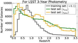
Figure 9.— True (green) and photometric (orange) redshift distributions of the test set of galaxies used for , along with the true redshift distribution of the training set (grey; scaled by $0.1$).

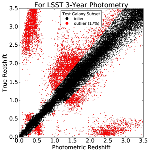
Figure 10.— True vs. photometric redshift for $50,000$ randomly chosen galaxies in the test set. Outliers (defined in the text) are colored red.

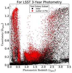
Figure 11.— Estimated photo-$z$ uncertainty ($\delta z_{\rm phot}$) vs. $z_{\rm phot}$ for a subset of test set galaxies. As in Fig. 10, outliers are colored red. For $z_{\rm phot}<0.5$, galaxies with a large uncertainty are mostly catastrophic outliers.

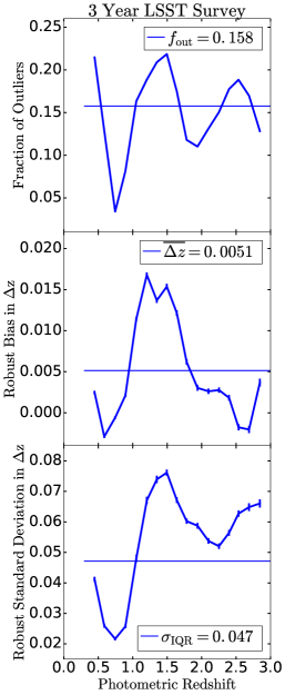
Figure 12.— Photo-$z$ performance measures: outlier fraction (top), bias (middle), and standard deviation (bottom). The average value across all bins is shown as a horizontal line.

6. Simulation

We use the simulation code from SNANA (Kessler et al., 2009b); an updated and detailed description of the simulation code is given in Kessler et al. (2019, hereafter K18). Here we give a brief and less technical description based on the overview shown in Fig. 13.

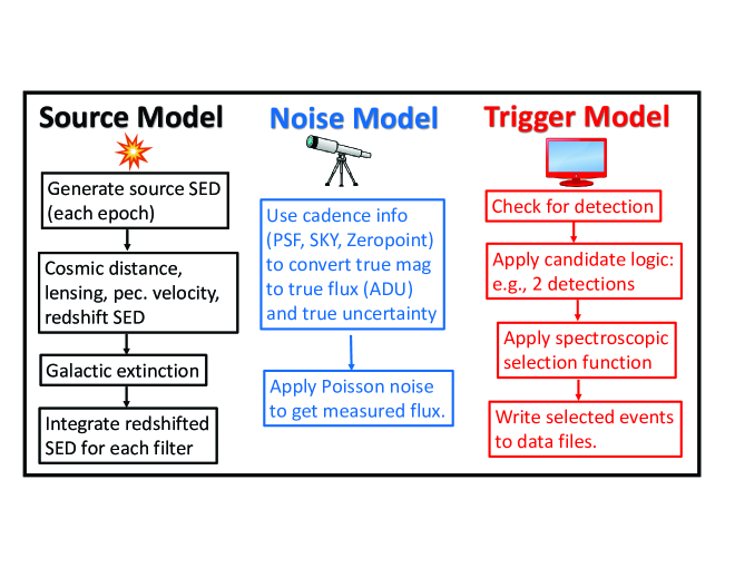
Figure 13.— Flow chart of stages in the SNANA simulation of extragalactic events.

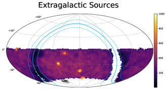
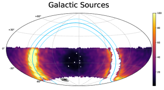
Figure 14.— Sky maps of  events shown in Hammer-Aitoff projection. The maps are generated with HEALPix NSIDE=32 and corresponds to a pixel size of 3.35 deg², or about 1/3 of the the LSST field of view (9.6 deg²). Top panel is for extragalactic sources; the 5 bright spots correspond to the DDFs, and the low-density bands overlap the Galactic plane (indicated with blue lines). Bottom panel is for Galactic sources.

6.1. Source Model

Here we describe the simulation stages under “Source Model” in Fig. 13. These stages correspond to extragalactic models described by rest-frame SEDs (§4). For Galactic models, these stages are replaced by precomputed magnitudes.

6.1.1 Model Enhancements

While the models in §4 are packaged as libraries the first step of the simulation is to provide a few model enhancements to avoid unphysical light-curve artifacts, and to include host-galaxy extinction. The first enhancement for SED-based models is related to the finite time range, typically a few hundred days. To avoid unphysical light-curve truncation, the magnitudes are linearly extrapolated. To reduce pathologies from noisy models at late times, the extrapolation is based on a least-squares fit to the last five days.

The next enhancement is to extrapolate fluxes into the far ultraviolet (UV) region so that $u$ band is defined at all redshifts. The blue edge of the $u$ band is ${\sim}3000$ Å, and thus at a maximum  redshift of $z=3.5$, this band probes the SED down to a wavelength of ${\sim}670$ Å. The SED models typically extend down to 1000 or 2000 Å, and therefore the $u$ band (and sometimes $g$ band) flux is not defined at high redshifts. Using the default SED models, these undefined passband fluxes would have been excluded from the output data files, and these drop-out artifacts could have been used as a feature in classification codes. To avoid UV drop-out artifacts in , and since real data will not have such artifacts, the SED flux at the bluest defined wavelength was linearly extrapolated down to zero flux at $500$ Å. This extrapolation was performed in each time bin for the SED grid. The resulting $u$-band model fluxes are negligible, and thus the reported $u$-band fluxes are dominated by sky noise fluctuations.

Data-driven models are assumed to include the effects of host-galaxy dust, which preferentially absorbs blue light and re-emits in the red, making the source appear redder from outside its host galaxy. The theoretically based models (MOSFiT-generated and KN) do not include dust, and thus for these models, we include extinction from dust described by $A_{V}$, the magnitude dimming at 5500 Å. The dimming at other wavelengths is determined by the same color law used to describe Milky Way reddening (Fitzpatrick, 1999). For all MOSFiT models except TDE, $A_{V}$ is selected from a “Galactic Line of Sight” distribution (Eq. 2 of Wood-Vasey et al. 2007) consisting of a Gaussian core ($\sigma=0.1$ mag) and exponential tail ($\tau=0.4$ mag). TDE  are expected to be near galactic centers, and thus only the exponential component is used. KN are expected to have large kicks, and thus the weight of the exponential component reduced by a factor of two.

The final enhancement is related to the probability of selecting nonrecurring Galactic events from the library of model light curves; this includes $\mu$Lens-Single and $\mu$Lens-Binary models. Events with longer duration are more likely to overlap with the LSST survey time, and we therefore select microlensing light curves with probability proportional to $T_{\rm LSST}+T_{\mu\rm Lens}$, where $T_{\rm LSST}$ is the survey duration (3 years) and $T_{\mu\rm Lens}$ is the duration of the microlensing event. Events with $T_{\mu\rm Lens}\ll T_{\rm LSST}$ have very nearly equal probabilities, while events with $T_{\mu\rm Lens}\gg T_{\rm LSST}$ have selection probability roughly proportional to $T_{\mu\rm Lens}$. For recurring Galactic events, each model light curve is selected with uniform probability.

6.1.2 Extragalactic Source Model and Photon Voyage to Earth

The extragalactic models in §4 describe the SED at a distance of 10 pc from the source. Here we describe the the lower 3 panels under “Source Model’ in Fig. 13: simulation of the photons’ journey through an expanding universe, through the Milky Way to the top of Earth’s atmosphere, and through the LSST passbands.

For distance $D$ within our Galaxy, the apparent brightness of a source follows the well known inverse-square law, $1/D^{2}$. For a source outside our Galaxy, the effect of cosmic distance in an expanding universe is characterized by replacing $D$ with a luminosity distance ($D_{L}$), which depends on cosmological model parameters as defined in Eq. 2 of K18. For , we used the following parameters to compute $D_{L}$: matter density $\Omega_{\rm M}=0.30$, dark energy density $\Omega_{\Lambda}=0.70$, and dark energy equation of state parameter $w=-1$. The apparent magnitude of each extragalactic source includes a distance modulus ($\mu$) defined as $\mu=-2.5\log(10{\rm pc}/D_{L}^{2})$, and therefore the intrinsic brightness for each model is defined at a distance of 10 pc.

As the light travels to earth, there are weak lensing effects in which the gravitational potential from galaxies near the light path trajectory can magnify or demagnify the source. To model this effect, a convergence distribution is determined from a 900 deg² patch of the MICECAT $N$-body simulation (Crocce et al., 2015). The magnification probability distribution is asymmetric and increases with redshift (§5.4 of K18); the root mean square (rms) of the magnification is roughly $0.05$ times the redshift.

Extragalactic sources reside in galaxies, and these galaxies have random “peculiar velocities” with respect to the cosmological redshift. The simulation selects a random velocity from a Gaussian distribution with $\sigma_{v}=300$ km/s (§5.5 of K18), which is equivalent to a redshift error of $\sigma_{z}=0.001$.

As the light enters the Milky Way, it travels through dust similar to the dust from the host galaxy. Instead of using the $A_{V}$ distribution from the host galaxy, we use a map of the color excess, $E(B-V)$, that has been precisely measured at every sky location (Schlegel et al., 1998). The extinction is given by $A_{V}=R_{V}\times E(B-V)$ where $R_{V}=3.1$. The color law from Fitzpatrick (1999) is used to determine the extinction as a function of wavelength. The uncertainty on $E(B-V)$ is $0.16{\times}E(B-V)$.

As the light reaches the top of our atmosphere, the redshifted SED is integrated over the wavelength range for each $ugrizy$ filter, resulting in six true fluxes. The conversion of true flux into measured flux is described below in §6.2.

6.2. Noise Model

Here we describe the simulation stages under “Noise Model” in Fig. 13. These stages are applied identically to both the extragalactic and Galactic models.

6.2.1 Model of Observing Conditions and Cadence

As described in §2, we simulate two components of the survey. The first component is the Wide-Fast-Deep (WFD), covering 17,950 deg² (44% of the entire sky). The second component is the set of Deep-Drilling Fields (DDF), which includes 5 telescope pointings covering 47.6 deg². For events passing the trigger (§6.3), the  sky densities for both the WFD and DDF are shown as HEALPix maps (Górski et al., 2005) in Fig. 14. Note that the extragalactic sources have nearly uniform coverage over the WFD area, while the Galactic events cluster much closer to the Galactic plane.

The sky coverage and sequence of observations are adapted from a baseline cadence published by LSST using the Operations Simulator, hereafter referred to as “OpSim” (Delgado et al., 2014; Delgado & Reuter, 2016; Reuter et al., 2016). OpSim includes a prototype scheduler that queues LSST observations to optimize science programs (§2) while accounting for a high-fidelity model of the telescope, and also accounting for real-time environmental factors such as weather, seeing, clouds, sky brightness, and maintenance downtime. We use OpSim version 3 that was available when the  data set was generated. The following discussion is for the 10-year survey, which was truncated to the first 3 years for the  simulation.

OpSim incorporates observing conditions with a time-dependent model of seeing, cloudiness, a dark sky spectrum, a model to compute the contribution of the moon to the sky brightness (Krisciunas & Schaefer, 1991), and a model of twilight behavior. The seeing model is based on two years of data at Cerro Pachon recorded every 5 minutes. The cloudiness was measured at Cerro Tololo during the same time period, with 0 being completely clear and 1 being completely cloudy. These data are repeated to cover the 10-year duration of LSST, and nearest-neighbor interpolation is used to determine values between measurements. A global open-shutter time constraint is applied to match the 10-year duration of LSST. Exposures of 30 seconds are scheduled when the sun altitude is below $-12$ deg (horizon is at 0 deg), the airmass is below $1.5$, and the distance to the moon (regardless of the phase) is greater than $30$ deg.

At any given time, the choice of science program and sky location is based on a greedy optimization algorithm to maximize the number of visits during a fixed block of time, and to also minimize slew time. The optimization algorithm tracks the fraction of completed visits for each science program in each spatial region, and computes the ideal fraction based on a uniform temporal distribution of visits. Priorities are adjusted to make the observed fractions match more closely to the ideal fractions. In addition, redder bands are given higher priority during twilight, bluer bands are preferred during dark time (no moon), and long temporal gaps are avoided for the transient science program. Finally, dithers up to 1.75 deg (Krughoff, 2016) are added to each WFD visit to cover chip gaps, spatially smooth the coadded depth, and randomize location and orientation dependence to reduce systematic biases in measurements of large scale structure and weak lensing (eg. see Carroll et al. 2014; Awan et al. 2016; LSST Science Collaboration et al. 2017). The final output is a publicly available LSST observation database of telescope pointings that includes sky coordinates, time of observation, bandpass, and quantities characterizing the observational conditions including airmass, point spread function (PSF), sky brightness, and $5\sigma$ depth.

For the public LSST observation database used for , the sky-brightness model was in development and tends to be overly conservative. We therefore applied an improved sky-brightness model from Yoachim et al. (2016), where the largest changes are in the $z$ and $y$ bands during twilight. On average, the resulting observation depths for  are a few tenths of a mag deeper compared to using the public database.

The final step is to translate the OpSim output (Biswas et al., 2019) into an observation library for the SNANA simulation (§6.2), and to truncate the 10-year survey to the first 3 years for . While an average observing season is ${\sim}6$ months, the sharp 3-year cutoff results in some short seasonal fragments in the third year. To reduce classification difficulties from this season-truncation artifact, seasonal fragments less than 30 days were not used.

The OpSim translation results in a 3-year observation history for 50,000 random sky locations within the WFD footprint; for DDF, 133 sky locations are used. The number of sky locations is a compromise between dense sky sampling and library size. The library sky density is ${\sim}2.8$ locations per square-degree, and thus for the 117 million generated events (Table 1), each sky location is re-used an average of ${\sim}2,300$ times. For the 3.5 million events passing the trigger, each sky location is re-used an average of ${\sim}70$ times. After co-adding observations within each night and passband, the average number of nightly passband visits over 3 years is 130 for WFD and 330 for DDF.

6.2.2 Instrumental Flux and Noise

Starting from the top of the atmosphere, the simulation would ideally trace the light through the atmosphere and the LSST instrument. While such simulations have been used for the LSST design (e.g., Tyson et al. 2014; Peterson et al. 2015; Rowe et al. 2015), they are very CPU intensive, especially for the 100 million sources that were generated for . Here we compute the observed flux and uncertainty from an “observation library” (§6.1 of K18), which consists of random sky locations and a list of observations at each location. For each observation the following information is included: modified Julian date (MJD), passband, sky noise, size of PSF, and zero point. The observation library for the SNANA simulation was created by translating the OpSim output described in §6.2.1. For a given true flux at the top of the atmosphere, the observation properties are used to compute the measured flux and uncertainty as described in §6.3 of K18.

In addition to modeling the flux from the source, we also model flux in the reference images, also commonly called template images. The fluxes in the data files are flux differences, $\Delta F$, corresponding to “search$-$reference” fluxes that are expected to be produced from the LSST image-subtraction pipeline (Bosch et al., 2018). For extragalactic transients, we assume that the source brightens after the reference images have been acquired, and therefore the reference flux is exactly equal to the search-image flux without the source. $\Delta F$ is therefore positive when the source is bright, and includes Gaussian sky noise. When the true source flux is zero, $\Delta F$ reduces to a Gaussian distribution centered at zero flux. For the Galactic and AGN models, the reference flux is modeled as an average of 4 snapshots taken over 4 consecutive days prior to the start of LSST operations. The resulting $\Delta F$ is therefore negative or positive.

The observed fluxes are determined in units of photoelectrons (GAIN=1). We simulate the common practice of “forced photometry,” where for each detected object the fluxes are measured at all previous and future observations at the same location. Simulated forced photometry means that for each object satisfying the  trigger (§6.3), all observations are recorded for the entire 3-year duration, regardless of the signal-to-noise ratio (S/N). The calibrated fluxes and uncertainties in the data files are on a common SNANA zero-point of 27.5. The calibrated flux does not correspond to a physical unit, but was arbitrarily chosen during the SDSS-II Supernova analysis (Kessler et al., 2009a), before SNANA existed, so that the calibrated SDSS flux has approximate units of photoelectrons.

Previous analyses have reported anomalous flux scatter from bright host galaxies; for DES, see Figs 9-10 of Kessler et al. (2015) and Fig. 5 of Brout et al. (2019a); for Pan-STARRS-1 (PS1), see Fig. 3 of Jones et al. (2017). For , we ignored these effects.

6.3. Trigger Model

Here we describe the simulation stages under “Trigger Model” in Fig. 13. These stages are applied identically to both the extragalactic and Galactic models.

Monitoring transient activity for every CCD pixel is not practical, and therefore we follow the common practice of using a software trigger to reduce the pixel data into catalog of objects with time-varying brightness. The trigger initiates photometric measurements on all previous and future observations for each object in the catalog. For the  trigger, we use assumptions based on the DES supernova program (DES-SN) described in Kessler et al. (2015, hereafter K15).

In our  simulation, a transient source must satisfy a trigger to be written out to the data files. While LSST plans to identify single-epoch detections for asteroid searches, we impose a transient trigger intended to reject moving objects by requiring 2 detections separated by at least 30 minutes. While asteroids with slow proper motions can still satisfy this trigger, our simulation does not include such objects. A detection is a group of CCD pixels with excess flux compared with a reference image, and a flux profile consistent with the PSF. We do not simulate pixel data, but instead use a DES-SN detection model from K15, which is based on analyzing artificial point sources overlaid on CCD images.

This model describes the detection efficiency as a function of true S/N (Fig. 8 of K15), ${\rm S/N}_{\rm true}$, which is computed from the true source brightness, sky noise, and PSF. The detection efficiency is 50% at ${\rm S/N}_{\rm true}{\sim}5$, and is nearly 100% at ${\rm S/N}_{\rm true}{\sim}10$. In addition to using these efficiency curves, we also required ${\rm S/N}_{\rm true}>3$ to avoid spurious detections on very low-S/N observations.

DES-SN only detected positive fluxes, meaning that the flux was required to be larger than the presurvey template flux. To allow for variables and longer-lived transients in LSST, a  detection is based on the absolute value of S/N, and thus increasing and decreasing fluxes (with respect to template flux) have the same probability of being detected.

6.4. Spectroscopically Confirmed Training Subset

A small subset of triggered events were flagged as spectroscopically identified and used for the training set. We loosely model the training set based on 4MOST, a spectroscopic instrument with 2400 fibers that is currently under construction, and a proposed “Time Domain Spectroscopic Survey” (Swann et al., 2019).

We used the DES characterization of the spectroscopic identification efficiency ($\epsilon_{\rm spec}$) as a function of peak $i$ band magnitude, $m_{i}$. Specifically, we used Fig. 4 of K18 where $\epsilon_{\rm spec}$ falls to 50% at around $m_{i}\simeq 22$ mag, but shifted the curve by 0.2 mag to reflect an assumption that the 4MOST spectrograph will be 0.2 mag deeper than spectrographs used for DES. The anticipated 4MOST improvements include better seeing and fiber efficiency. The expected number of spectroscopic classifications for 4MOST is below $10^{4}$, and thus in addition to the $i$-band dependent $\epsilon_{\rm spec}$, prescale fractions in Table 3 were also applied. A prescale of 0.008, for example, means that that the $\epsilon_{\rm spec}$ curve (Fig. 4 of K18) is multiplied by 0.008. The total number of events in the training set is 7,846, and almost 3/4 of the training set events are in the WFD. The largest classes in the training set are SNIa (30%) and SNII (15%).

Table 3 Prescale Fractions Applied to Spectroscopic Identification Efficiency

Model	Prescale for
Num: Name	DDF	WFD
90: SNIa	0.500	0.003
42: SNII	1.000	0.008
62: SNIbc	1.000	0.008
67: SNIa-91bg	1.000	0.008
52: SNIax	1.000	0.008
64: KN	1.000	1.000
95: SLSN-I	1.000	0.008
15: TDE	1.000	0.200
88: AGN	1.000	0.008
92: RRL	0.300	0.0008
65: M-dwarf	1.000	0.008
16: EB	1.000	0.008
53: Mira	0.500	0.020
6: $\mu$Lens-Single	0.500	0.100

6.5. Photometric Redshift from Host Galaxy

For extragalactic transients, we use the photometric redshift library described in §5, where each galaxy includes a true redshift ($z_{\rm true}$), photometric redshift ($z_{\rm phot}$), and photometric redshift uncertainty ($\delta z_{\rm phot}$). For a true source redshift generated from the rate model, $z_{\rm source}$, the simulation picks a random galaxy from the library satisfying

$$|z_{\rm true}-z_{\rm source}|<0.01+0.05z_{\rm source}~{},$$ (11)

where the tolerance provides a broader distribution of selected galaxies. Defining $z_{\rm phot,ran}$ as the photometric redshift associated with the randomly selected galaxy, the photometric redshift for the source is

$$z_{\rm phot}=z_{\rm phot,ran}+(z_{\rm source}-z_{\rm true})~{},$$ (12)

and $\delta z_{\rm phot}$ is the reported 68% confidence uncertainty. For more details, see §6.2 of K18.

6.6. Spectroscopic Redshifts from Host Galaxy

Using the 4MOST instrument capabilities as a guide, we expect to obtain accurate spectroscopic redshifts ($z_{\rm spec}$) for a small fraction of host galaxies. Figure 15 shows the $z_{\rm spec}$ efficiency vs. redshift for the WFD and DDF, and these efficiency curves were used in the simulation to select a random subset of 140,000 events (4% of sample) with a $z_{\rm spec}$ measurement. Both efficiencies are set to one at very low redshift ($z<0.02$) to avoid photo-$z$ artifacts, and for $z>0.02$ the efficiency drops to connect with the 4MOST-based efficiency. The WFD efficiency drops to 1% around $z\sim 0.5$. The DDF efficiency drops to 1% around $z\sim 1.1$; many repeat DDF visits are stacked, resulting in higher efficiency compared with WFD.

Figure 15.— Efficiency vs. redshift for measuring an accurate spectroscopic redshift from the host galaxy. The DDF spectra are stacked from multiple visits, and thus the DDF efficiency is higher compared to WFD.

6.7. Special Features for

Here we describe a few simulation features that were implemented specifically for . First, all fluxes are corrected for the measured Galactic extinction to prevent professional astronomers from using their domain knowledge to gain an advantage over the Kaggle community. The correction is based on measured $E(B-V)$, which includes random Gaussian scatter about the true value with $\sigma=0.16E(B-V)$. We also require $E(B-V)<3$ to limit the extinction values.

The next issue concerns the default option of reporting fluxes only within a well-defined time window to limit the output data volume. To prevent participants from using the duration of reported fluxes as a classification feature, we report a flux and uncertainty for every LSST observation over the 3 year duration. An approximate light-curve duration, however, can be obtained from a boolean flag that was set for each detection (§6.3).

For LSST, the CCD pixels are expected to saturate for signals above $\sim 10^{5}$ photoelectrons, which corresponds to sources brighter than about $16^{\rm th}$ mag. The  team decided that accounting for saturated observations is an unnecessary distraction for the challenge, and therefore we simulated a saturation level at $12^{\rm th}$ mag, or 4 mag brighter than nominal. In addition, we removed the small number of saturated observations that remained.

Finally, the information released about  did not mention that the publicly available SNANA simulation code was used to generate the data files. Nonetheless, we took the following precautions: removed -related indicators from the SNANA source code and documentation (e.g., name of cluster, names of rare models, etc…), never publicly mentioned the name of the “Midway” computer cluster used to generate the data files, and protected all -related files on the Midway cluster.

6.8. Re-using Model SEDs and Light Curves

For most of the models, the number of generated events greatly exceeds the number of SED time series for extragalactic models, or light curves for Galactic models. As an extreme case, 220,200 events were generated for the EB model, but there are only 500 model light curves to choose from. When an SED time series or light curve is re-used, the simulated light curve is different for several reasons beyond random Poisson noise. For extragalactic events (except AGN), each event has a different redshift, host-galaxy extinction, sky location, and cadence. For Galactic events (and AGN), each event has a different sky location, cadence, initial phase, and reference-image flux.

6.9. Validation

All of the models combined include roughly a million SEDs, and a non-trivial task was to validate the simulated output, and in particular to minimize unphysical artifacts from software bugs and from artifacts in the newly created model libraries.

Our primary tool was visual inspection of simulated light curves, a task shared among a dozen astronomers from the -validation team. Artifacts were either fixed by the model developer, or fixed with upgrades to the SNANA simulation. The other main validation technique was to inspect distributions of sky density, redshift, and luminosity functions. Kaggle performed their own internal tests, and they found an interesting artifact that we could not explain: among the 453 million observations included in the data set, they found about 100 pairs of duplicate fluxes. The duplicates were from different classes, and only occurred when the true flux is zero.

Our final, and perhaps most important validation, is that the SNANA simulation has been previously used in numerous published measurements of cosmological parameters where the simulation accurately predicts distributions observed in the data. Example data-simulation comparisons have been shown for DES (Fig. 7 in Brout et al. 2019b), PS1 (Fig. 4 in Jones et al. 2017 and Fig. 7 in Scolnic et al. 2018b), and SDSS & SNLS (Fig. 1-2 in Kessler et al. 2013).

While preparing this manuscript, we identified 6 mistakes in the simulation: (1) rate discontinuity at $z{=}1$ (§4.1.2), (2) lack of variation in SNIa-91bg model (§4.2.2), (3) luminosity function too narrow for SNII-NMF (§4.4.2), (4) included SLSN-I models fainter than $-21$ mag (§4.6.2), (5) incorrect M-dwarf $b$-dependence in the DDF (footnote 12 in §4), and (6) applied incorrect ${\rm S/N}_{\rm true}>3$ requirement for the trigger (footnote 36 in §6.3). These mistakes were identical in the training and test sets and therefore did not cause leakage, and these mistakes did not compromise our goals for the Kaggle competition. However, such mistakes could have led to subtle data/simulation discrepancies if there had been real data to make such comparisons.

6.10. Light Curves from  Data Set

A few extragalactic $i$-band light curves from the  data set are shown in Fig. 16, spanning a range of 170 days. The first three panels show different supernova classes in the DDF, where the different transient time-scales are visually apparent. The lower 2 panels show SLSN-I and KN light curves in the WFD survey. Although the DDF area is much smaller than WFD, note the vastly superior cadence in the DDF. Negative fluxes are due to small (or zero) source flux combined with Poisson sky fluctuations resulting in smaller sky level in the search image compared with the template used for image subtraction. A few Galactic $i$-band light curves from the  data set (DDF) are shown in Fig. 17, spanning the entire 3 years. Note that the $\mu$Lens-Single model is a transient with finite duration. Large negative fluxes are due to the source flux in the presurvey template image being larger than the flux measured in the search image.

Figure 16.— Example extragalactic light curves in $i$-band. The model name, observing mode (DDF or WFD) and redshift are shown on each panel. The MJD axis is shifted so that zero corresponds to peak bolometric flux. The dotted horizontal line through zero is to guide the eye. Each light curve was selected with redshift $z{\sim}0.2$ to visually compare flux and width. Note that the WFD light curves (lower two panels) have significantly fewer observations compared with the DDF light curves (upper three panels).

Figure 17.— Example Galactic light curves in $i$-band (DDF only). The model name is shown on each panel. The MJD axis is shifted so that zero is the start of LSST observing. The dotted horizontal line through zero is to guide the eye.

6.11.  Data Files

The  data files are described on the Kaggle platform (footnote 2), and here is a brief summary. The metadata for each event include: integer object identifier, sky coordinates (R.A., decl.), host-galaxy photo-$z$ and its uncertainty (§6.5), host-galaxy spectroscopic redshift for a small fraction of events (§6.6), distance modulus computed from the photo-$z$, and Galactic extinction estimate, $E(B-V)$ (§6.1.2). For the training set (§6.4), the model class is also provided. The following information is provided for each observation: integer object identifier, Modified Julian Date (MJD), passband ($ugrizy$), measured flux, flux uncertainty, and boolean flag for detection (§6.3).

7. Discussion & Conclusion

There are two primary products resulting from the  challenge. The first product is a set of 18 models of transients and variables within a unified analysis framework, an enormous leap over previous simulations. These models are publicly available in PLAsTiCC Modelers (2019), and each model is packaged as a separate library so that any simulation code can be applied.

The second product is a new set of classification techniques (R.Hložek et al. 2019, in preparation). The winning method was based on augmenting the training set by degrading well-measured light curves; this increased the training set from 8,000 to 270,000 events. Next, the light curves were smoothed with a Gaussian process method, and 200 features were extracted. Finally, the features were trained with a machine-learning method called “Light Gradient Boosting Machine” (LightGBM). Shortly after the end of the challenge, Kaggle participants shared their methods, codes, and training products. Using different machine-learning methods on the augmented training set, participants obtained classification scores better than the original winning score, an encouraging sign that a combination of methods can significantly improve classification.

To improve classification beyond , improvements are needed for both the models and the simulation. In the spirit of the original community call for models, we invite improvements to existing models, and development of new models that were not part of . A critically needed simulation improvement is to associate extragalactic transients to host-galaxy properties. It is also important to replace DES observing properties, e.g., detection efficiency versus S/N and spectroscopic selection vs. peak $i$-band magnitude, with a characterization of LSST and expected spectroscopic follow-up. Finally, LSST’s difference-imaging pipeline may result in photometric light curves with artifacts that have not been included in . These artifacts include catastrophic outliers, excess noise on bright galaxies, and saturated observations. To test the robustness of classifiers to photometric artifacts, it is important to characterize the LSST difference-imaging pipeline and model this behavior in the SNANA simulation.

The  challenge has provided a unique opportunity to combine efforts from a wide range of astronomical communities, and also from Kaggle’s data challenge community where more than 1000 people participated. The  data set was designed to reflect our best understanding of the universe and the LSST instrumental performance. This effort has resulted in significant improvements in simulation and analysis tools, which will be critical to address the scientific challenges of the LSST era.

8. Acknowledgements

This paper has undergone internal review in the LSST Dark Energy Science Collaboration; we are grateful to internal reviewers Rachel Mandelbaum, Simon Krughoff, and Peter Nugent for their valuable input to this manuscript. We are also grateful to the anonymous referee for a thorough review.

This work was supported in part by the Kavli Institute for Cosmological Physics at the University of Chicago through grant NSF PHY-1125897 and an endowment from the Kavli Foundation and its founder Fred Kavli. R.K. is supported by DOE grant DE-AC02-76CH03000, and NASA grant NNG17PX03C. This work was completed in part with resources provided by the University of Chicago Research Computing Center. This research at Rutgers University (M.D., S.W.J.) is supported by DOE award DE-SC0011636 and NSF award AST-1615455. D.O.J. is supported by a Gordon and Betty Moore Foundation postdoctoral fellowship at the University of California, Santa Cruz. S.G acknowledges the support from the FCT project PTDC/FIS-AST/31546/2017. D.C. acknowledges the John Templeton Foundation New Frontiers Program grant No. 37426 (University of Chicago) and FP050136-B (Cornell University); NSF grant No. 1417132. A.J.C acknowledges support by the U.S. Department of Energy, Office of Science, under Award Number DESC-0011635, and partial support from the Washington Research Foundation and the DIRAC Institute. S.A.R. and J.D.R.P. acknowledge support from the National Aeronautics and Space Administration through a NASA EPSCoR Research Infrastructure Development award administered by the South Carolina Space Grant Consortium.

We thank Kaggle for selecting PLAsTiCC to run under the Research Competition category, providing expertise and guidance throughout the implementation of this project and for funding the main prizes. We also thank the entire data science community responsible for solidifying the tradition of data challenges and, specially, all the Kaggle participants who engaged in .  was funded through LSST Corporation grant award #2017-03 and administered by the University of Toronto.

The DESC acknowledges ongoing support from the Institut National de Physique Nucléaire et de Physique des Particules in France; the Science & Technology Facilities Council in the United Kingdom; and the Department of Energy, the National Science Foundation, and the LSST Corporation in the United States. DESC uses resources of the IN2P3 Computing Center (CC-IN2P3–Lyon/Villeurbanne - France) funded by the Centre National de la Recherche Scientifique; the National Energy Research Scientific Computing Center, a DOE Office of Science User Facility supported by the Office of Science of the U.S. Department of Energy under Contract No. DE-AC02-05CH11231; STFC DiRAC HPC Facilities, funded by UK BIS National E-infrastructure capital grants; and the UK particle physics grid, supported by the GridPP Collaboration. This work was performed in part under DOE Contract DE-AC02-76SF00515.

We thank Carlton Baugh and the The Institute for Computational Cosmology for access to their simulated mock catalogs. This material is based upon work supported in part by the National Science Foundation through Cooperative Agreement 1258333 managed by the Association of Universities for Research in Astronomy (AURA), and the Department of Energy under Contract No. DE-AC0276SF00515 with the SLAC National Accelerator Laboratory. Additional LSST funding comes from private donations, grants to universities, and in-kind support from LSSTC Institutional Members.

Author Contributions are Listed Below

R. Kessler: co-lead project, simulation software, generate  data set, data curation, three models (SNIa, SNII, SNIbc), writing, project administration, and supervision. G. Narayan: KN & microlens models, data curation, validation, Kaggle-participant liaison, editing, project administration, and supervision. A. Avelino: two microlens models and writing. E. Bachelet: single-lens microlensing model and writing. R. Biswas: observation library, editing, project administration, and supervision. D. F. Chernoff: string-microlens model and writing. A. Connolly: host-galaxy photo-$z$ model. M. Dai: SNIax model and validation. S. Daniel: three models (AGN, M-dwarf, RR Lyrae) and writing. R. Di Stefano: two microlens models and writing. M. R. Drout: SNIbc model and writing. L.Galbany: validation, SNIa-91bg & SNII-NMF models, writing, and editing. S.González-Gaitán: SNIa-91bg & SNII-NMF models, writing, and editing. M.L.Graham: host-galaxy photo-$z$ model and writing. R. Hložek: co-lead project, funding acquisition, Mira model, writing, editing, project administration, and supervision. E. E. O. Ishida: Kaggle liaison, validation, editing, project administration, and supervision. J. Guillochon: seven models (IIn, Ibc, SLSN-I, TDE, ILOT, CaRT, PISN). S. W. Jha: SNIax model and editing. D. O. Jones: SN1a-91bg model and editing. K. Mandel: SNIa model. A. O’Grady: Mira Model. C. M. Peters: validation and editing. J. R. Pierel: SNII & SNIbc models. K. A. Ponder: validation and editing. A. Prša: eclipsing binary model and writing. S. Rodney: SNII,SNIbc models. V. A. Villar: seven models (IIn, Ibc, SLSN-I, TDE, ILOT, CaRT, PISN) and writing.

Appendix A Overview of MOSFiT Code

To produce SEDs for transient sources we use MOSFiT: the Modular Open-Source Fitter for Transients, a Python-based package which generates Monte Carlo ensembles of semi-analytical, one-zone SED models (Guillochon et al., 2018). Utilizing a number of potential energy sources (e.g., ⁵⁶Ni decay), MOSFiT can simulate SEDs for a number of astrophysical transients across a broad range of parameters. This is done by segmenting the model into a number of “modular” components: e.g., the input energy source, diffusion, a photosphere, etc. See Fig. 3 of Guillochon et al. 2018 for example kilonovae and superluminous supernovae models.

References

- Abbott et al. (2016) Abbott, B. P., Abbott, R., Abbott, T. D., et al. 2016, ApJ, 832, L21
- Abbott et al. (2017a) —. 2017a, Nature, 551, 85
- Abbott et al. (2017b) —. 2017b, ApJ, 848, L13
- Abbott et al. (2017c) —. 2017c, Phys. Rev. Lett., 119, 161101
- Abbott et al. (2017d) —. 2017d, ApJ, 848, L12
- Afonso et al. (2000) Afonso, C., Alard, C., Albert, J. N., et al. 2000, ApJ, 532, 340
- Alcock et al. (1993) Alcock, C., Akerlof, C. W., Allsman, R. A., et al. 1993, Nature, 365, 621
- Anderson et al. (2014) Anderson, J. P., González-Gaitán, S., Hamuy, M., et al. 2014, ApJ, 786, 67
- Angus et al. (2016) Angus, C. R., Levan, A. J., Perley, D. A., et al. 2016, MNRAS, 458, 84
- Angus et al. (2019) Angus, C. R., Smith, M., Sullivan, M., et al. 2019, MNRAS, 487, 2215
- Arcavi et al. (2017) Arcavi, I., Hosseinzadeh, G., Howell, D. A., et al. 2017, Nature, 551, 64
- Awan et al. (2016) Awan, H., Gawiser, E., Kurczynski, P., et al. 2016, ApJ, 829, 50
- Bachelet et al. (2017) Bachelet, E., Norbury, M., Bozza, V., & Street, R. 2017, AJ, 154, 203
- Baker et al. (2017) Baker, T., Bellini, E., Ferreira, P. G., et al. 2017, Physical Review Letters, 119, 251301
- Ball et al. (2008) Ball, N. M., Brunner, R. J., Myers, A. D., et al. 2008, ApJ, 683, 12
- Barkat et al. (1967) Barkat, Z., Rakavy, G., & Sack, N. 1967, Physical Review Letters, 18, 379
- Barnes & Hernquist (1991) Barnes, J. E. & Hernquist, L. E. 1991, ApJ, 370, L65
- Baumann & McAllister (2015) Baumann, D. & McAllister, L. 2015, Inflation and String Theory, Cambridge Monographs on Mathematical Physics (Cambridge University Press)
- Beaulieu (2018) Beaulieu, J.-P. 2018, Universe, 4, 61
- Bellm et al. (2019) Bellm, E. C., Kulkarni, S. R., Graham, M. J., et al. 2019, PASP, 131, 018002
- Betoule et al. (2014) Betoule, M., Kessler, R., Guy, J., et al. 2014, A&A, 568, A22
- Biswas et al. (2019) Biswas, R., Daniel, S. F., Hložek, R., Kim, A. G., & Yoachim, P. 2019, arXiv e-prints, arXiv:1905.02887
- Blandford & McKee (1982) Blandford, R. D. & McKee, C. F. 1982, ApJ, 255, 419
- Blondin et al. (2012) Blondin, S., Matheson, T., Kirshner, R. P., et al. 2012, AJ, 143, 126
- Bloomfield & Chernoff (2014) Bloomfield, J. K. & Chernoff, D. F. 2014, Phys. Rev., D89, 124003
- Bond et al. (2001) Bond, I. A., Abe, F., Dodd, R. J., et al. 2001, MNRAS, 327, 868
- Bosch et al. (2018) Bosch, J., AlSayyad, Y., Armstrong, R., et al. 2018, arXiv e-prints
- Brout et al. (2019a) Brout, D., Sako, M., Scolnic, D., et al. 2019a, ApJ, 874, 106
- Brout et al. (2019b) Brout, D., Scolnic, D., Kessler, R., et al. 2019b, ApJ, 874, 150
- Brown et al. (2014) Brown, P. J., Breeveld, A. A., Holland, S., Kuin, P., & Pritchard, T. 2014, Ap&SS, 354, 89
- Brown et al. (2009) Brown, P. J., Holland, S. T., Immler, S., et al. 2009, AJ, 137, 4517
- Carroll et al. (2014) Carroll, C. M., Gawiser, E., Kurczynski, P. L., et al. 2014, in Proc. SPIE, Vol. 9149, Observatory Operations: Strategies, Processes, and Systems V, 91490C
- Catelan & Smith (2015) Catelan, M. & Smith, H. A. 2015, Pulsating Stars
- Chang et al. (2015) Chang, S.-W., Byun, Y.-I., & Hartman, J. D. 2015, ApJ, 814, 35
- Chatzopoulos et al. (2012) Chatzopoulos, E., Wheeler, J. C., & Vinko, J. 2012, ApJ, 746, 121
- Chatzopoulos et al. (2013) Chatzopoulos, E., Wheeler, J. C., Vinko, J., Horvath, Z. L., & Nagy, A. 2013, ApJ, 773, 76
- Chatzopoulos et al. (2016) Chatzopoulos, E., Wheeler, J. C., Vinko, J., et al. 2016, ApJ, 828, 94
- Chen et al. (2018) Chen, H.-Y., Fishbach, M., & Holz, D. E. 2018, Nature, 562, 545
- Chernoff (2009) Chernoff, D. F. 2009, ArXiv:0908.4077
- Chernoff & Tye (2007) Chernoff, D. F. & Tye, S. H. H. 2007, ArXiv:0709.1139
- Chernoff & Tye (2015) —. 2015, Int. J. Mod. Phys., D24, 1530010
- Chernoff & Tye (2018) —. 2018, JCAP, 1805, 002
- Chevalier & Irwin (2011) Chevalier, R. A. & Irwin, C. M. 2011, ApJ, 729, L6
- Chomiuk et al. (2011) Chomiuk, L., Chornock, R., Soderberg, A. M., et al. 2011, ApJ, 743, 114
- Chornock et al. (2006) Chornock, R., Filippenko, A. V., Branch, D., et al. 2006, PASP, 118, 722
- Conley et al. (2008) Conley, A., Sullivan, M., Hsiao, E. Y., et al. 2008, ApJ, 681, 482
- Connolly et al. (2014) Connolly, A. J., Angeli, G. Z., Chandrasekharan, S., et al. 2014, in Proc. SPIE, Vol. 9150, Modeling, Systems Engineering, and Project Management for Astronomy VI, 915014
- Connolly et al. (2010) Connolly, A. J., Peterson, J., Jernigan, J. G., et al. 2010, in Proc. SPIE, Vol. 7738, Modeling, Systems Engineering, and Project Management for Astronomy IV, 77381O
- Contreras et al. (2018) Contreras, C., Phillips, M. M., Burns, C. R., et al. 2018, ApJ, 859, 24
- Cooke et al. (2012) Cooke, J., Sullivan, M., Gal-Yam, A., et al. 2012, Nature, 491, 228
- Coulter et al. (2017) Coulter, D. A., Foley, R. J., Kilpatrick, C. D., et al. 2017, Science, 358, 1556
- Crocce et al. (2015) Crocce, M., Castander, F. J., Gaztañaga, E., Fosalba, P., & Carretero, J. 2015, MNRAS, 453, 1513
- Davenport et al. (2014) Davenport, J. R. A., Hawley, S. L., Hebb, L., et al. 2014, ApJ, 797, 122
- de Jaeger et al. (2015) de Jaeger, T., González-Gaitán, S., Anderson, J. P., et al. 2015, ApJ, 815, 121
- De Lucia et al. (2006) De Lucia, G., Springel, V., White, S. D. M., Croton, D., & Kauffmann, G. 2006, MNRAS, 366, 499
- Delgado & Reuter (2016) Delgado, F. & Reuter, M. A. 2016, in Proc. SPIE, Vol. 9910, Observatory Operations: Strategies, Processes, and Systems VI, 991013
- Delgado et al. (2014) Delgado, F., Saha, A., Chandrasekharan, S., et al. 2014, in Proc. SPIE, Vol. 9150, Modeling, Systems Engineering, and Project Management for Astronomy VI, 915015
- DES Collaboration et al. (2019) DES Collaboration et al. 2019, ApJ, 872, L30
- Di Stefano (2000) Di Stefano, R. 2000, ApJ, 541, 587
- Dilday et al. (2008) Dilday, B., Kessler, R., Frieman, J. A., et al. 2008, ApJ, 682, 262
- Dominik (1998) Dominik, M. 1998, A&A, 329, 361
- Duchêne & Kraus (2013) Duchêne, G. & Kraus, A. 2013, Annual Review of Astronomy and Astrophysics, 51, 269
- Eldridge & Maund (2016) Eldridge, J. J. & Maund, J. R. 2016, MNRAS, 461, L117
- Evans & Kochanek (1989) Evans, C. R. & Kochanek, C. S. 1989, ApJ, 346, L13
- Filippenko et al. (1992) Filippenko, A. V., Richmond, M. W., Branch, D., et al. 1992, AJ, 104, 1543
- Fitzpatrick (1999) Fitzpatrick, E. L. 1999, PASP, 111, 63
- Folatelli et al. (2016) Folatelli, G., Van Dyk, S. D., Kuncarayakti, H., et al. 2016, ApJ, 825, L22
- Foley et al. (2013) Foley, R. J., Challis, P. J., Chornock, R., et al. 2013, ApJ, 767, 57
- Foley et al. (2009) Foley, R. J., Chornock, R., Filippenko, A. V., et al. 2009, AJ, 138, 376
- Freedman (2017) Freedman, W. L. 2017, Nature Astronomy, 1, 0121
- Friedman et al. (2015) Friedman, A. S., Wood-Vasey, W. M., Marion, G. H., et al. 2015, ApJS, 220, 9
- Frohmaier et al. (2018) Frohmaier, C., Sullivan, M., Maguire, K., & Nugent, P. 2018, ApJ, 858, 50
- Gaia Collaboration et al. (2018) Gaia Collaboration et al. 2018, A&A, 616, A1
- Gal-Yam et al. (2009) Gal-Yam, A., Mazzali, P., Ofek, E. O., et al. 2009, Nature, 462, 624
- Galbany et al. (2016) Galbany, L., Hamuy, M., Phillips, M. M., et al. 2016, AJ, 151, 33
- Galbany et al. (2017) Galbany, L., Mora, L., González-Gaitán, S., et al. 2017, MNRAS, 468, 628
- González-Gaitán et al. (2014) González-Gaitán, S., Hsiao, E. Y., Pignata, G., et al. 2014, ApJ, 795, 142
- González-Gaitán et al. (2011) González-Gaitán, S., Perrett, K., Sullivan, M., et al. 2011, ApJ, 727, 107
- González-Gaitán et al. (2015) González-Gaitán, S., Tominaga, N., Molina, J., et al. 2015, MNRAS, 451, 2212
- Górski et al. (2005) Górski, K. M., Hivon, E., Banday, A. J., et al. 2005, ApJ, 622, 759
- Gould (2004) Gould, A. 2004, ApJ, 606, 319
- Graham et al. (2018) Graham, M. L., Connolly, A. J., Ivezić, Ž., et al. 2018, AJ, 155, 1
- Graur et al. (2017) Graur, O., Bianco, F. B., Modjaz, M., et al. 2017, ApJ, 837, 121
- Guillochon et al. (2018) Guillochon, J., Nicholl, M., Villar, V. A., et al. 2018, ApJS, 236, 6
- Guillochon et al. (2017) Guillochon, J., Parrent, J., Kelley, L. Z., & Margutti, R. 2017, ApJ, 835, 64
- Guinan et al. (1998) Guinan, E. F., Fitzpatrick, E. L., DeWarf, L. E., et al. 1998, ApJ, 509, L21
- Guo et al. (2015) Guo, X., Esin, A., Di Stefano, R., & Taylor, J. 2015, ApJ, 809, 182
- Guy et al. (2010) Guy, J., Sullivan, M., Conley, A., et al. 2010, A&A, 523, A7
- Hachinger et al. (2009) Hachinger, S., Mazzali, P. A., Taubenberger, S., Pakmor, R., & Hillebrandt, W. 2009, MNRAS, 399, 1238
- Hamuy & Pinto (2002) Hamuy, M. & Pinto, P. A. 2002, ApJ, 566, L63
- Hawley et al. (2003) Hawley, S. L., Allred, J. C., Johns-Krull, C. M., et al. 2003, ApJ, 597, 535
- Hawley et al. (2014) Hawley, S. L., Davenport, J. R. A., Kowalski, A. F., et al. 2014, ApJ, 797, 121
- Hilton (2011) Hilton, E. J. 2011, PhD thesis, University of Washington
- Hilton et al. (2011) Hilton, E. J., Hawley, S. L., Kowalski, A. F., & Holtzman, J. 2011, in Astronomical Society of the Pacific Conference Series, Vol. 448, 16th Cambridge Workshop on Cool Stars, Stellar Systems, and the Sun, ed. C. Johns-Krull, M. K. Browning, & A. A. West, 197
- Hilton et al. (2010) Hilton, E. J., West, A. A., Hawley, S. L., & Kowalski, A. F. 2010, AJ, 140, 1402
- Hirata et al. (1987) Hirata, K., Kajita, T., Koshiba, M., et al. 1987, Phys. Rev. Lett., 58, 1490
- Hoeflich et al. (2017) Hoeflich, P., Hsiao, E. Y., Ashall, C., et al. 2017, ApJ, 846, 58
- Holtzman et al. (2008) Holtzman, J. A., Marriner, J., Kessler, R., et al. 2008, AJ, 136, 2306
- Hopkins et al. (2006) Hopkins, P. F., Hernquist, L., Cox, T. J., et al. 2006, ApJS, 163, 1
- Hounsell et al. (2018) Hounsell, R., Scolnic, D., Foley, R. J., et al. 2018, ApJ, 867, 23
- Howell et al. (2005) Howell, D. A., Sullivan, M., Perrett, K., et al. 2005, ApJ, 634, 1190
- Hoyle et al. (2018) Hoyle, B., Gruen, D., Bernstein, G. M., et al. 2018, MNRAS, 478, 592
- Ireland et al. (2008) Ireland, M. J., Scholz, M., & Wood, P. R. 2008, MNRAS, 391, 1994
- Ireland et al. (2011) —. 2011, MNRAS, 418, 114
- Ishida et al. (2019) Ishida, E. E. O., Beck, R., González-Gaitán, S., et al. 2019, MNRAS, 483, 2
- Ivezić et al. (2008) Ivezić, Ž., Kahn, S. M., Tyson, J. A., et al. 2008, ArXiv e-prints
- Jha (2017) Jha, S. W. Type Iax Supernovae, 375
- Jiang et al. (2016) Jiang, N., Dou, L., Wang, T., et al. 2016, ApJ, 828, L14
- Jones et al. (2017) Jones, D. O., Scolnic, D. M., Riess, A. G., et al. 2017, ApJ, 843, 6
- Jurić et al. (2008) Jurić, M., Ivezić, Ž., Brooks, A., et al. 2008, ApJ, 673, 864
- Kasen et al. (2017) Kasen, D., Metzger, B., Barnes, J., Quataert, E., & Ramirez-Ruiz, E. 2017, Nature, 551, 80
- Kasen et al. (2011) Kasen, D., Woosley, S., & Heger, A. 2011, ApJ, 734, 102
- Keller & Wood (2006) Keller, S. C. & Wood, P. R. 2006, ApJ, 642, 834
- Kessler et al. (2010) Kessler, R., Bassett, B., Belov, P., et al. 2010, PASP, 122, 1415
- Kessler et al. (2009a) Kessler, R., Becker, A. C., Cinabro, D., et al. 2009a, ApJS, 185, 32
- Kessler et al. (2009b) Kessler, R., Bernstein, J. P., Cinabro, D., et al. 2009b, PASP, 121, 1028
- Kessler et al. (2019) Kessler, R., Brout, D., D’Andrea, C. B., et al. 2019, MNRAS, 485, 1171
- Kessler et al. (2013) Kessler, R., Guy, J., Marriner, J., et al. 2013, ApJ, 764, 48
- Kessler et al. (2015) Kessler, R., Marriner, J., Childress, M., et al. 2015, AJ, 150, 172
- Kirk et al. (2016) Kirk, B., Conroy, K., Prša, A., et al. 2016, AJ, 151, 68
- Kochanek (2016) Kochanek, C. S. 2016, MNRAS, 461, 371
- Kowalski et al. (2009) Kowalski, A. F., Hawley, S. L., Hilton, E. J., et al. 2009, AJ, 138, 633
- Kozyreva et al. (2018) Kozyreva, A., Kromer, M., Noebauer, U. M., & Hirschi, R. 2018, MNRAS, 479, 3106
- Krisciunas et al. (2017) Krisciunas, K., Contreras, C., Burns, C. R., et al. 2017, AJ, 154, 211
- Krisciunas & Schaefer (1991) Krisciunas, K. & Schaefer, B. E. 1991, PASP, 103, 1033
- Krughoff (2016) Krughoff, K. 2016, Hexagonal Dithering for LSST, https://zenodo.org/record/55701
- Kurucz (1993) Kurucz, R. 1993, ATLAS9 Stellar Atmosphere Programs and 2 km/s grid. Kurucz CD-ROM No. 13. Cambridge, Mass.: Smithsonian Astrophysical Observatory, 1993., 13
- La Franca et al. (2014) La Franca, F., Bianchi, S., Ponti, G., Branchini, E., & Matt, G. 2014, ApJ, 787, L12
- Lattimer & Schramm (1974) Lattimer, J. M. & Schramm, D. N. 1974, ApJ, 192, L145
- Leistedt & Hogg (2017) Leistedt, B. & Hogg, D. W. 2017, ApJ, 838, 5
- Leloudas et al. (2009) Leloudas, G., Stritzinger, M. D., Sollerman, J., et al. 2009, A&A, 505, 265
- Li et al. (2011) Li, W., Chornock, R., Leaman, J., et al. 2011, MNRAS, 412, 1473
- Li et al. (2003) Li, W., Filippenko, A. V., Chornock, R., et al. 2003, PASP, 115, 453
- Lipunov et al. (2017) Lipunov, V. M., Gorbovskoy, E., Kornilov, V. G., et al. 2017, ApJ, 850, L1
- Livne & Arnett (1995) Livne, E. & Arnett, D. 1995, ApJ, 452, 62
- LSST Science Collaboration et al. (2009) LSST Science Collaboration et al. 2009, arXiv:0912.0201
- LSST Science Collaboration et al. (2017) —. 2017, ArXiv:1708.04058
- Lunnan et al. (2014) Lunnan, R., Chornock, R., Berger, E., et al. 2014, ApJ, 787, 138
- Lunnan et al. (2017) Lunnan, R., Kasliwal, M. M., Cao, Y., et al. 2017, ApJ, 836, 60
- Lyman et al. (2013) Lyman, J. D., James, P. A., Perets, H. B., et al. 2013, MNRAS, 434, 527
- Lyman et al. (2018) Lyman, J. D., Taddia, F., Stritzinger, M. D., et al. 2018, MNRAS, 473, 1359
- MacLeod et al. (2010) MacLeod, C. L., Ivezić, Ž., Kochanek, C. S., et al. 2010, ApJ, 721, 1014
- Madau & Dickinson (2014) Madau, P. & Dickinson, M. 2014, ARA&A, 52, 415
- Magee et al. (2016) Magee, M. R., Kotak, R., Sim, S. A., et al. 2016, A&A, 589, A89
- Malz et al. (2018) Malz, A., Hložek, R., Allam, Jr, T., et al. 2018, ArXiv:1809.11145
- Mao (2012) Mao, S. 2012, Research in Astronomy and Astrophysics, 12, 947
- Mao & Di Stefano (1995) Mao, S. & Di Stefano, R. 1995, ApJ, 440, 22
- Mao & Paczynski (1991) Mao, S. & Paczynski, B. 1991, ApJ, 374, L37
- Maoz et al. (2014) Maoz, D., Mannucci, F., & Nelemans, G. 2014, ARA&A, 52, 107
- Matheson et al. (2008) Matheson, T., Kirshner, R. P., Challis, P., et al. 2008, AJ, 135, 1598
- McCrum et al. (2015) McCrum, M., Smartt, S. J., Rest, A., et al. 2015, MNRAS, 448, 1206
- Merson et al. (2013) Merson, A. I., Baugh, C. M., Helly, J. C., et al. 2013, MNRAS, 429, 556
- Milisavljevic et al. (2017) Milisavljevic, D., Patnaude, D. J., Raymond, J. C., Drout, M. R., Margutti, R., Kamble, A., Chornock, R., Guillochon, J., Sanders, N. E., Parrent, J. T., Lovisari, L., Chilingarian, I. V., Challis, P., Kirshner, R. P., Penny, M. T., Itagaki, K., Eldridge, J. J., & Moriya, T. J. 2017, ApJ, 846, 50
- Miller et al. (2017) Miller, A. A., Kasliwal, M. M., Cao, Y., et al. 2017, ApJ, 848, 59
- Mockler et al. (2019) Mockler, B., Guillochon, J., & Ramirez-Ruiz, E. 2019, ApJ, 872, 151
- Moe & Di Stefano (2017) Moe, M. & Di Stefano, R. 2017, ApJS, 230, 15
- Mróz et al. (2017) Mróz, P., Udalski, A., Skowron, J., et al. 2017, Nature, 548, 183
- Nicholl et al. (2017) Nicholl, M., Guillochon, J., & Berger, E. 2017, ApJ, 850, 55
- Nicholl et al. (2015) Nicholl, M., Smartt, S., Jerkstrand, A., Sim, S., et al. 2015, ApJ, 807, L18
- Nugent et al. (2002) Nugent, P., Kim, A., & Perlmutter, S. 2002, PASP, 114, 803
- Paczynski (1986) Paczynski, B. 1986, ApJ, 304, 1
- Pan et al. (2012) Pan, T., Loeb, A., & Kasen, D. 2012, MNRAS, 423, 2203
- Perets et al. (2010) Perets, H. B., Gal-Yam, A., Mazzali, P. A., et al. 2010, Nature, 465, 322
- Perlmutter et al. (1999) Perlmutter, S., Alfdering, G., Goldhaber, G., et al. 1999, ApJ, 517, 565
- Peterson et al. (2015) Peterson, J. R., Jernigan, J. G., Kahn, S. M., et al. 2015, ApJS, 218, 14
- Phillips (1993) Phillips, M. M. 1993, ApJ, 413, L105
- Phillips et al. (2007) Phillips, M. M., Li, W., Frieman, J. A., et al. 2007, PASP, 119, 360
- Pierel et al. (2018) Pierel, J. D. R., Rodney, S., Avelino, A., et al. 2018, PASP, 130, 114504
- Planck Collaboration et al. (2018) Planck Collaboration et al. 2018, arXiv:1807.06205
- PLAsTiCC Modelers (2019) PLAsTiCC Modelers. 2019, PLAsTiCC Models, https://doi.org/10.5281/zenodo.2612896
- PLAsTiCC Team (2018) PLAsTiCC Team. 2018, ArXiv:1810.00001
- PLAsTiCC Team (2019) —. 2019, Unblinded Data from PLAsTiCC, https://doi.org/10.5281/zenodo.2535747
- Plewa et al. (2004) Plewa, T., Calder, A. C., & Lamb, D. Q. 2004, ApJ, 612, L37
- Polin et al. (2019) Polin, A., Nugent, P., & Kasen, D. 2019, ApJ, 873, 84
- Prajs et al. (2017) Prajs, S., Sullivan, M., Smith, M., et al. 2017, MNRAS, 464, 3568
- Prša et al. (2011) Prša, A., Batalha, N., Slawson, R. W., et al. 2011, AJ, 141, 83
- Prša et al. (2016) Prša, A., Conroy, K. E., Horvat, M., et al. 2016, ApJS, 227, 29
- Quimby et al. (2011) Quimby, R., Kulkarni, S., Kasliwal, M., et al. 2011, Nature, 474, 487
- Quimby et al. (2013) Quimby, R. M., Yuan, F., Akerlof, C., & Wheeler, J. C. 2013, MNRAS, 431, 912
- Raghavan et al. (2010) Raghavan, D., McAlister, H. A., Henry, T. J., et al. 2010, ApJS, 190, 1
- Rees (1988) Rees, M. J. 1988, Nature, 333, 523
- Refsdal (1964) Refsdal, S. 1964, MNRAS, 128, 295
- Reuter et al. (2016) Reuter, M. A., Cook, K. H., Delgado, F., Petry, C. E., & Ridgway, S. T. 2016, in Proc. SPIE, Vol. 9911, Modeling, Systems Engineering, and Project Management for Astronomy VI, 991125
- Richardson et al. (2014) Richardson, D., Jenkins III, R. L., Wright, J., & Maddox, L. 2014, The Astronomical Journal, 147, 118
- Riess et al. (1998) Riess, A. G., Filippenko, A. V., Challis, P., et al. 1998, AJ, 116, 1009
- Riess et al. (2016) Riess, A. G., Macri, L. M., Hoffmann, S. L., et al. 2016, ApJ, 826, 56
- Riess et al. (1996) Riess, A. G., Press, W. H., & Kirshner, R. P. 1996, ApJ, 473, 88
- Risaliti & Lusso (2017) Risaliti, G. & Lusso, E. 2017, Astronomische Nachrichten, 338, 329
- Robin et al. (2003) Robin, A. C., Reylé, C., Derrière, S., & Picaud, S. 2003, Astronomy & Astrophysics, 409, 523
- Rowe et al. (2015) Rowe, B. T. P., Jarvis, M., Mandelbaum, R., et al. 2015, Astronomy and Computing, 10, 121
- Rust (1974) Rust, B. W. 1974, PhD thesis, Oak Ridge National Lab., TN.
- Sadeh et al. (2016) Sadeh, I., Abdalla, F. B., & Lahav, O. 2016, PASP, 128, 104502
- Sahu et al. (2008) Sahu, D. K., Tanaka, M., Anupama, G. C., et al. 2008, ApJ, 680, 580
- Sako et al. (2018) Sako, M., Bassett, B., Becker, A. C., et al. 2018, PASP, 130, 064002
- Sanders et al. (1988) Sanders, D. B., Soifer, B. T., Elias, J. H., et al. 1988, ApJ, 325, 74
- Schlegel et al. (1998) Schlegel, D. J., Finkbeiner, D. P., & Davis, M. 1998, ApJ, 500, 525
- Scolnic & Kessler (2016) Scolnic, D. & Kessler, R. 2016, ApJ, 822, L35
- Scolnic et al. (2018a) Scolnic, D., Kessler, R., Brout, D., et al. 2018a, ApJ, 852, L3
- Scolnic et al. (2018b) Scolnic, D. M., Jones, D. O., Rest, A., et al. 2018b, ApJ, 859, 101
- Scovacricchi et al. (2016) Scovacricchi, D., Nichol, R. C., Bacon, D., Sullivan, M., & Prajs, S. 2016, MNRAS, 456, 1700
- Sesar et al. (2010) Sesar, B., Ivezić, Ž., Grammer, S. H., et al. 2010, ApJ, 708, 717
- Sharma et al. (2011) Sharma, S., Bland-Hawthorn, J., Johnston, K. V., & Binney, J. 2011, ApJ, 730, 3
- Sheldon et al. (2012) Sheldon, E. S., Cunha, C. E., Mandelbaum, R., Brinkmann, J., & Weaver, B. A. 2012, ApJS, 201, 32
- Shen et al. (2018) Shen, K. J., Kasen, D., Miles, B. J., & Townsley, D. M. 2018, ApJ, 854, 52
- Shen et al. (2015) Shen, Y., Brandt, W. N., Dawson, K. S., et al. 2015, ApJS, 216, 4
- Silk & Rees (1998) Silk, J. & Rees, M. J. 1998, A&A, 331, L1
- Silverman et al. (2012) Silverman, J. M., Foley, R. J., Filippenko, A. V., et al. 2012, MNRAS, 425, 1789
- Smartt et al. (2009) Smartt, S. J., Eldridge, J. J., Crockett, R. M., & Maund, J. R. 2009, MNRAS, 395, 1409
- Smith et al. (2016) Smith, M., Sullivan, M., D’Andrea, C., et al. 2016, ApJ, 818, L8
- Smith et al. (2018) Smith, M., Sullivan, M., Nichol, R. C., et al. 2018, ApJ, 854, 37
- Soares-Santos et al. (2017) Soares-Santos, M., Holz, D. E., Annis, J., et al. 2017, ApJ, 848, L16
- Soszyński et al. (2009) Soszyński, I., Udalski, A., Szymański, M. K., et al. 2009, Acta Astronomica, 59, 239
- Speagle et al. (2016) Speagle, J. S., Capak, P. L., Eisenstein, D. J., Masters, D. C., & Steinhardt, C. L. 2016, MNRAS, 461, 3432
- Springel et al. (2005) Springel, V., White, S. D. M., Jenkins, A., et al. 2005, Nature, 435, 629
- Stanishev et al. (2007) Stanishev, V., Taubenberger, S., Blanc, G., et al. 2007, in American Institute of Physics Conference Series, Vol. 924, The Multicolored Landscape of Compact Objects and Their Explosive Origins, ed. T. di Salvo, G. L. Israel, L. Piersant, L. Burderi, G. Matt, A. Tornambe, & M. T. Menna, 336–341
- Stritzinger et al. (2015) Stritzinger, M. D., Valenti, S., Hoeflich, P., et al. 2015, A&A, 573, A2
- Strolger et al. (2015) Strolger, L.-G., Dahlen, T., Rodney, S. A., et al. 2015, ApJ, 813, 93
- Swann et al. (2019) Swann, E., Sullivan, M., Carrick, J., et al. 2019, The Messenger, 175, 58
- Tanaka et al. (2018) Tanaka, M., Coupon, J., Hsieh, B.-C., et al. 2018, Publications of the Astronomical Society of Japan, 70, S9
- Tanvir et al. (2017) Tanvir, N. R., Levan, A. J., González-Fernández, C., et al. 2017, ApJ, 848, L27
- The LIGO Scientific Collaboration & the Virgo Collaboration (2018) The LIGO Scientific Collaboration & the Virgo Collaboration. 2018, arXiv:1811.12907
- Torres et al. (2010) Torres, G., Andersen, J., & Giménez, A. 2010, Astronomy and Astrophysics Review, 18, 67
- Tripp (1998) Tripp, R. 1998, A&A, 331, 815
- Tsapras (2018) Tsapras, Y. 2018, Geosciences, 8, 365
- Tyson et al. (2014) Tyson, J. A., Sasian, J., Gilmore, K., et al. 2014, in Proc. SPIE, Vol. 9154, High Energy, Optical, and Infrared Detectors for Astronomy VI, 915415
- Udalski et al. (1992) Udalski, A., Szymanski, M., Kaluzny, J., Kubiak, M., & Mateo, M. 1992, Acta Astronomica, 42, 253
- Udalski et al. (1994) Udalski, A., Szymanski, M., Mao, S., et al. 1994, ApJ, 436, L103
- Valenti et al. (2009) Valenti, S., Pastorello, A., Cappellaro, E., et al. 2009, Nature, 459, 674
- Valenti et al. (2017) Valenti, S., Sand, D. J., Yang, S., et al. 2017, ApJ, 848, L24
- Van Dyk (2017) Van Dyk, S. D. 2017, Philosophical Transactions of the Royal Society of London Series A, 375, 20160277
- van Velzen (2018) van Velzen, S. 2018, ApJ, 852, 72
- Vanden Berk et al. (2001) Vanden Berk, D. E., Richards, G. T., Bauer, A., et al. 2001, AJ, 122, 549
- Vilenkin (1981) Vilenkin, A. 1981, Phys. Rev., D23, 852
- Vilenkin (1984) —. 1984, Astrophys. J., 282, L51
- Vilenkin & Shellard (2000) Vilenkin, A. & Shellard, E. P. S. 2000, Cosmic Strings and Other Topological Defects, 578
- Villar et al. (2017) Villar, V. A., Berger, E., Metzger, B. D., & Guillochon, J. 2017, ApJ, 849, 70
- Villar et al. (2018) Villar, V. A., Nicholl, M., & Berger, E. 2018, ApJ, 869, 166
- Walkowicz et al. (2011) Walkowicz, L. M., Basri, G., Batalha, N., et al. 2011, AJ, 141, 50
- Wanderman & Piran (2015) Wanderman, D. & Piran, T. 2015, MNRAS, 448, 3026
- Watson et al. (2011) Watson, D., Denney, K. D., Vestergaard, M., & Davis, T. M. 2011, ApJ, 740, L49
- Wells et al. (2017) Wells, M., Prša, A., Jones, L., & Yoachim, P. 2017, PASP, 129, 065003
- West et al. (2008) West, A. A., Hawley, S. L., Bochanski, J. J., et al. 2008, AJ, 135, 785
- West et al. (2011) West, A. A., Morgan, D. P., Bochanski, J. J., et al. 2011, AJ, 141, 97
- Wood-Vasey et al. (2007) Wood-Vasey, W. M., Miknaitis, G., Stubbs, C. W., et al. 2007, ApJ, 666, 694
- Woosley & Weaver (1986) Woosley, S. E. & Weaver, T. A. 1986, ARA&A, 24, 205
- Yoachim et al. (2016) Yoachim, P., Coughlin, M., Angeli, G. Z., et al. 2016, in Society of Photo-Optical Instrumentation Engineers (SPIE) Conference Series, Vol. 9910, Observatory Operations: Strategies, Processes, and Systems VI, 99101A
- York et al. (2000) York, D. G., Adelman, J., Anderson, Jr., J. E., et al. 2000, AJ, 120, 1579
- Zheng et al. (2008) Zheng, C., Romani, R. W., Sako, M., et al. 2008, AJ, 135, 1766