Note on a solution to domain wall problem with the
Lazarides-Shafi mechanism in axion dark matter models

Abstract

Axion is a promising candidate of dark matter. After the Peccei-Quinn symmetry breaking, axion strings are formed and attached by domain walls when the temperature of the universe becomes comparable to the QCD scale. Such objects can cause cosmological disasters if they are long-lived. As a solution for it, the Lazarides-Shafi mechanism is often discussed through introduction of a new non-Abelian (gauge) symmetry. We study this mechanism in detail and show configuration of strings and walls. Even if Abelian axion strings with a domain wall number greater than one are formed in the early universe, each of them is split into multiple Alice axion strings due to a repulsive force between the Alice strings even without domain wall. When domain walls are formed as the universe cools down, a single Alice string can be attached by a single wall because a vacuum is connected by a non-Abelian rotation without changing energy. Even if an Abelian axion string attached by domain walls are created due to the Kibble Zurek mechanism at the chiral phase transition, such strings are also similarly split into multiple Alice strings attached by walls in the presence of the domain wall tension. Such walls do not form stable networks since they collapse by the tension of the walls, emitting axions.

I Introduction

The standard model successfully explains various phenomena in experiments. However there exist several unsolved problems. One of the problems is the strong CP problem. We may have a CP violating term in QCD:

$$\mathcal{L}=\theta\frac{g_{s}^{2}}{32\pi^{2}}G^{a\mu\nu}\tilde{G}^{a}_{\mu\nu},$$ (1)

where $\theta$ is a constant parameter, $g_{s}$ is the strong coupling constant, $G^{a}_{\mu\nu}$ is the gluon field strength, and $\tilde{G}^{a}_{\mu\nu}$ is its dual. Measurements of the neutron electric dipole moment gives a constraint that $|\theta|\lesssim 10^{-10}$ Baker:2006ts , while a naive expectation is that $|\theta|={\cal O}(1)$. Without any mechanisms, this would require a fine-tuning. The problem can be naturally solved if one introduces the Peccei-Quinn (PQ) mechanism with a global $U(1)$ symmetry denoted by $U(1)_{\rm PQ}$ Peccei:1977hh ; Peccei:1977ur ; Weinberg:1977ma . After the spontaneous $U(1)_{\rm PQ}$ breaking, a pseudo Nambu-Goldstone boson called the QCD axion appears. When the $U(1)_{\rm PQ}$ symmetry is explicitly broken by QCD instanton effect via chiral anomaly between $U(1)_{\rm PQ}$ and QCD, the axion vacuum is at a CP-conserving minimum of the potential and the axion solves the strong CP problem. The axion decay constant $f_{a}$ is of order the $U(1)_{\rm PQ}$ symmetry breaking scale, and the so-called axion window is given by

$$10^{9}\leavevmode\nobreak\ {\rm GeV}\lesssim f_{a}\lesssim 10^{12}\leavevmode\nobreak\ {\rm GeV}.$$ (2)

The lower bound comes from the SN 1987A neutrino burst duration Raffelt:2006cw . The upper bound comes from the dark matter abundance by the misalignment mechanism without a tuning of the initial misalignment, in which the coherent oscillation of the axion around the vacuum accounts for the abundance Preskill:1982cy ; Abbott:1982af ; Dine:1982ah . See e.g. Refs. Kim:2008hd ; Kawasaki:2013ae for reviews.

Physics of axion is related to the history of the universe. Below temperature of $1$ GeV, QCD instantons breaks the $U(1)_{\rm PQ}$ to $\mathbb{Z}_{N_{\rm DW}}$ symmetry, where $N_{\rm DW}$ is an integer called the domain wall number, then there appear $N_{\rm DW}$ vacua. Along with the PQ symmetry breaking, domain walls attached to strings are formed Kibble:1982dd ; Vilenkin:1982ks ; Everett:1982nm ; Zeldovich:1974uw ; Preskill:1992ck once one of the vacua is chosen. The cosmological scenario depends on when the breakdown of the PQ symmetry takes place. If the PQ symmetry is broken before or during inflation, strings and walls are inflated away because the axion field value becomes homogeneous over the scale of Hubble horizon after inflation. They cannot affect on cosmological observations, however, there exist a stringent constraint on isocurvature perturbation produced by the axion during the inflation Akrami:2018odb . If the PQ symmetry is broken after inflation, such a constraint does not exist, but walls and strings may survive until late time and can affect on evolution of the universe. We will focus on the latter case in this paper.

A stability of walls attached to strings is known to depend on $N_{\rm DW}$, which is related to a topological charge. For $N_{\rm DW}=1$, the domain wall attached to a string collapses owing to its tension, emitting axions. On top of the misalignment, axions produced by their decays accounts for a fraction of the dark matter abundance Kawasaki:2014sqa ; Klaer:2017ond . For $N_{\rm DW}>1$, the domain walls attached to a string constitute complex networks, which are called string-domain wall networks. The walls in the network pull each other with their tensions and they do not shrink to a point, thus networks can be long-lived. They eventually dominate the energy density of the universe beyond those of radiation and matter, and conflict with the standard cosmology. This is called a domain wall problem Zeldovich:1974uw .

For a solution to the domain wall problem, several ideas have been proposed so far Vilenkin:1981zs ; Lazarides:1982tw ; Kawasaki:2015lpf ; Sato:2018nqy . Among them, we will focus on an axion model associated with a continuous non-Abelian gauge symmetry proposed by Lazarides-Shafi Lazarides:1982tw . One might think that a topologically stable domain wall is formed when $\mathbb{Z}_{N_{\rm DW}}$ symmetry is spontaneously broken by choosing the vacuum. However, when the non-Abelian symmetry are also spontaneously broken at the same time and a combination of $\mathbb{Z}_{N_{\rm DW}}$ and the broken non-Abelian rotation can make the vacuum invariant, the vacua are also continuously connected also by the non-Abelian group without changing energy. This is because the non-Abelian rotation is equivalent to a travel in the space of would-be NG modes. Then, a topological property of such a domain wall for any $N_{\rm DW}$ becomes trivial like in a case with $N_{\rm DW}=1$. Hence domain wall problem is solved. This is called the Lazarides-Shafi mechanism.

However, behaviors of strings and walls in the mechanism has not been much discussed in literatures, while the authors of Ref. Sato:2018nqy discussed the decay of Abelian axion strings to Alice axion strings to solve the domain wall problem based on the mechanism. In this model, we may have $N_{\rm DW}=2$ and a single Axion string is attached by two domain walls, seemingly having a domain wall problem. The Alice string produced by the decay plays a crucial role to realize a situation similar to the $N_{\rm DW}=1$ case, in which one Alice string is attached by one domain wall. Hence the network is unstable in the presence of the domain wall tension. (See Refs. Abrikosov:1956sx ; Nielsen:1973cs for Abelian string and also Refs. Hindmarsh:1994re ; Vilenkin:2000jqa for reviews of cosmic strings.)

Alice strings have a peculiar property that when the electric charge of a charged particle encircles around an Alice string, it changes its sign Schwarz:1982ec ; Kiskis:1978ed . Other peculiar propeties such as a topological obstruction, a non-local charge called the Chesire charge, and non-Abelian statistics, have been studied in the literature Alford:1990mk ; Alford:1990ur ; Alford:1992yx ; Preskill:1990bm ; Bucher:1993jj ; Bucher:1992bd ; Lo:1993hp ; Striet:2000bf . While a typical Alice string is present in an $SO(3)$ gauge theory with scalar fields in the fiveplet representation (a traceless symmetric tensor), recently it has been found that a $U(1)\times SO(3)$ gauge theory with complex triplet scalar fields also admits an Alice string, which is a Bogomol’nyi-Prasad-Sommerfield state Bogomolny:1975de ; Prasad:1975kr and is stable, thereby possible to be embedded into supersymmetric theories Chatterjee:2017jsi ; Chatterjee:2017hya . A global analog was known in the context of Bose-Einstein condensates in condensed matter physics Leonhardt:2000km ; Ruostekoski:2003qx ; Kobayashi:2011xb ; Kawaguchi:2012ii . The Alice axion string proposed in Ref. Sato:2018nqy is the case that only the $U(1)$ part is global identified with axion, while the $SU(2)$ part is a gauge symmetry.

In this paper, we show why the domain wall problem is solved physically in more detail, focusing on dynamics of domain walls and two types of axion strings. It is found that even if Abelian axion strings are formed in the early universe, the string decays into multiple Alice axion strings owing to a repulsive force between the Alice strings. When domain walls are formed at the chiral phase transition as the universe cools down, a single Alice axion string is attached by a single wall because a vacuum is connected by a non-Abelian rotation without changing energy. Such walls do not form stable networks since they collapse owing to the tension of the walls, emitting axions similarly to the $N_{\rm DW}=1$ case. Also, at the chiral phase transition, two types of domain walls may be created by the Kibble-Zurek mechanism Kibble:1976sj ; Zurek:1985qw , and can be glued along an Abelian axion string. The Abelian axion string is pulled by these domain walls and is splitted into multiple Alice axion strings, each of which is attached by one domain wall. In either of these cases, the domain wall problem can be solved.

The rest of this paper is organized as follows. In Sec. II, we briefly review the QCD axion and domain wall problem. In Sec. III, we introduce an axion model with heavy quarks and a new gauge symmetry for solving the domain wall problem. In Sec. IV, properties of strings and domain walls are studied. In Sec. V, we study domain walls attached to strings. Sec. VI is devoted to discussion and conclusions.

II Review of the QCD axion and domain wall problem

In this section, we review the QCD axion based on the Kim-Shifman-Vainstein-Zakharov (KSVZ) model Kim:1979if ; Shifman:1979if and domain wall problem for simplicity. (The Dine-Fischler-Srednicki-Zhitnitsky (DFSZ) model Dine:1981rt ; Zhitnitsky:1980tq can be also discussed in a similar way.) Let us consider a coupling

$$\mathcal{L}=y\bar{Q}^{i}\Phi Q^{i}+{\rm h.c.}\leavevmode\nobreak\ \leavevmode\nobreak\ \leavevmode\nobreak\ (i=1,2,\cdots,N_{\rm DW}).$$ (3)

Here, $(\bar{Q},\leavevmode\nobreak\ Q)$ are $N_{\rm DW}$ pairs of extra heavy quark in the $SU(3)_{c}$ gauge symmetry, and $\Phi$ is a complex scalar singlet under the Standard Model gauge symmetry. This coupling is invariant under the global $U(1)_{\rm PQ}$ symmetry:

$$\bar{Q}\to e^{-i\theta}\bar{Q}\leavevmode\nobreak\ ,\leavevmode\nobreak\ \leavevmode\nobreak\ Q\to Q\leavevmode\nobreak\ ,\leavevmode\nobreak\ \leavevmode\nobreak\ \Phi\to e^{i\theta}\Phi\leavevmode\nobreak\ .$$ (4)

Here $\theta$ is a transformation parameter. Suppose that after inflation $\Phi$ develops vacuum expectation value (VEV) $\eta$ and the $U(1)_{\rm PQ}$ is spontaneously broken down. Thus the scalar field is parametrized as

$$\Phi=\sqrt{2}\left(\eta+\frac{\sigma}{2}\right)\exp\left(i\frac{a}{2\eta}\right).$$ (5)

Here $\sigma$ is supposed to be stabilized and we neglect it throughout this paper, $a$ is the QCD axion. Note that a $U(1)_{\rm PQ}$ rotation of $a\to a+2\pi\cdot(2\eta)$ is a symmetry. All pairs of extra quarks obtain heavy mass $\sqrt{2}y\eta\times e^{i\frac{a}{2\eta}}$. After integrating out extra quarks with the rotation of $\bar{Q}Q\to e^{-i\frac{a}{2\eta}}\bar{Q}Q$, we obtain

$$\mathcal{L}=\frac{a}{f_{a}}\frac{g_{s}^{2}}{32\pi^{2}}G^{a\mu\nu}\tilde{G}^{a}_{\mu\nu},\leavevmode\nobreak\ \leavevmode\nobreak\ \leavevmode\nobreak\ {\rm where}\leavevmode\nobreak\ f_{a}\equiv\frac{2\eta}{N_{\rm DW}}$$ (6)

via the chiral anomaly between $U(1)_{\rm PQ}$ and $SU(3)_{c}$. Thus $\langle a\rangle=0$ means the CP-conserving vacuum. After the chiral symmetry breaking in QCD, gluons and light quarks are integrated out, and the axion potential can be written as

$$V(a)\simeq m_{\pi}^{2}f_{\pi}^{2}\left(1-\cos\left(\frac{a}{f_{a}}\right)\right)\sim\cos\left(N_{\rm DW}\frac{a}{2\eta}\right).$$ (7)

Here, $m_{\pi}$ is the pion mass and $f_{\pi}$ is the pion decay constant. As desired, $\langle a\rangle=0$ is obtained in the vacuum and the strong CP problem is then solved. The axion mass is given by

$$m_{a}\simeq\frac{m_{\pi}f_{\pi}}{f_{a}}\simeq 6\times 10^{-4}{\rm eV}\bigg{(}\frac{10^{10}{\rm GeV}}{f_{a}}\bigg{)}.$$ (8)

Note that $a\to a+2\pi f_{a}$ is the ${\mathbb{Z}}_{N_{\rm DW}}$ symmetry against the above potential, in addition to the original larger symmetry of $a\to a+2\pi N_{\rm DW}f_{a}$. Thus, there exist $N_{\rm DW}$ vacua. Once one of the vacua is chosen, ${\mathbb{Z}}_{N_{\rm DW}}$ symmetry is spontaneously broken and topologically stable domain walls (attached to Abelian strings) appear between vacua for $N_{\rm DW}>1$. When one classically travels from a vacuum to the next one in the axion field space, it is necessary to climb the potential energy. The walls pull each other with their tensions and they do not shrink to a point, thus can be long-lived. The presence of stable domain walls conflict with the standard cosmology, because they eventually dominate the energy density of the universe beyond those of radiation and matter. It is verified in simulations that domain walls survive until late time for $N_{\rm DW}>1$, while they decay for $N_{\rm DW}=1$ or in the presence of bias potential for $N_{\rm DW}>1$ Kawasaki:2014sqa ; Klaer:2017ond . For $N_{\rm DW}=1$, the axion dark matter abundance produced by decays of walls and strings is estimated as

$$\Omega_{a}h^{2}\sim 10^{-2}\bigg{(}\frac{f_{a}}{10^{10}{\rm GeV}}\bigg{)}^{1.19}.$$ (9)

III The model with a non-Abelian gauge symmetry

Following the Ref. Sato:2018nqy , we explain the model to implement the Lazarides-Shafi mechanism in the KSVZ case. We shall start with the hidden $SU(2)_{H}$ gauge theory on top of the global $U(1)_{\rm PQ}$ symmetry. The Lagrangian is given as

$$\mathcal{L}=-\frac{1}{2}\hbox{\rm Tr}F_{\mu\nu}F^{\mu\nu}+\hbox{\rm Tr}|D_{\mu}\Phi|^{2}-V(\Phi)+(y\bar{Q}\Phi Q+{\rm h.c.})$$ (10)

where $F_{\mu\nu}$ is the $SU(2)_{H}$ gauge field strength, $\Phi$ is a complex adjoint scalar field and $(\bar{Q},Q)$ are extra quarks charged also under both $SU(2)_{H}$ and $U(1)_{\rm PQ}$. Their charge assignment against $(SU(3)_{c},SU(2)_{H},U(1)_{\rm PQ})$ is as follows: $\Phi:(1,3,1),\leavevmode\nobreak\ \bar{Q}:(\bar{3},\bar{2},-1)$ and $Q:(3,2,0)$. $SU(2)_{H}$ adjoint fields can be expanded with the $SU(2)$ generators $\tau^{a}=\frac{1}{2}\sigma^{a}$ as $\Phi=\phi^{a}\tau^{a}$ and $A_{\mu}=A_{\mu}^{a}\tau^{a}$, and the covariant derivative is defined as $D_{\mu}\Phi=\partial_{\mu}\Phi-ig[A_{\mu},\Phi]$. Here $g$ is the $SU(2)_{H}$ gauge coupling. The potential for $\Phi$ is given as

$$V(\Phi)=\frac{\lambda_{1}}{2}\left(\hbox{\rm Tr}(\Phi^{\dagger}\Phi)-2\eta^{2}\right)^{2}+\frac{\lambda_{2}}{2}\hbox{\rm Tr}\big{(}[\Phi,\Phi^{\dagger}]^{2}\big{)}.$$ (11)

This is an usual potential for complex adjoint scalar field that breaks $U(1)_{\rm PQ}\times SU(2)_{H}$ spontaneously. Later we will consider an explicit violation term for $U(1)_{\rm PQ}$, which is relevant to axion mass and domain wall construction. The ground state is given by the solution of the equations

$$\hbox{\rm Tr}\Phi^{\dagger}\Phi=2\eta^{2},\qquad[\Phi,\Phi^{\dagger}]=0.$$ (12)

The vacuum solution we may generally choose as

$$\langle\Phi\rangle=2\eta\tau^{1}=\eta\sigma^{1}.$$ (13)

The VEV breaks $U(1)_{\rm PQ}$ and $SU(2)_{H}$, then there exists the unbroken $U(1)_{H}$ gauge symmetry with a generator of $\tau^{1}$. This vacuum is invariant under $O(2)$ rather than $SO(2)$. The elements are given as

$$H=\{(1,e^{i\alpha\tau^{1}}),(-1,i(c_{1}\sigma^{2}+c_{2}\sigma^{3})e^{i\alpha\tau^{1}})\}.$$ (14)

Here $\alpha,\leavevmode\nobreak\ c_{1,2}$ are parameters and the conditon of $c_{1}^{2}+c_{2}^{2}=1$ is satisfied. The first entry of each element of $H$ is $U(1)_{\rm PQ}$ and the second entry is the element of $U(1)\subset SU(2)_{H}$ group, which can act as adjoint representation on $\langle\Phi\rangle$. The first element is usual element of $U(1)_{H}\subset O(2)$ connected to identity element $(1,1)$. However, the second element is a non-trivial $\mathbb{Z}_{2}$. Note that $e^{i\pi Q_{\rm PQ}}=-1$ for $Q_{\rm PQ}=1$, where $Q_{\rm PQ}$ is the PQ charge of the $\Phi$, and $e^{i\pi\tau^{a}}=i\sigma^{a}$ for $a=2,3$: The first entry is $\pi$ rotation of $U(1)_{\rm PQ}$ and the part of second entry $i(c_{1}\sigma^{2}+c_{2}\sigma^{3})$ gives $\pi$ rotation of broken $SU(2)_{H}$ around an axis orthogonal to $\tau^{1}$. So the second element of $H$ is referred to the disconnected elements of $O(2)$.

More specifically we may describe the symmetry breaking procedure as

$$G=U(1)_{\rm PQ}\times\frac{SU(2)_{H}}{\mathbb{Z}_{2}}\simeq U(1)_{\rm PQ}\times SO(3)_{H}\longrightarrow H=\mathbb{Z}_{2}\ltimes U(1)_{H}\simeq O(2),$$ (15)

where $\ltimes$ denotes the semi-direct product because the $\mathbb{Z}_{2}$ caused by $\pi$ rotation in the above discussion does not commute with the unbroken $U(1)_{H}$ generated by $\tau^{1}$. The vacuum manifold is found to be

$$\frac{G}{H}=\frac{U(1)_{\rm PQ}\times SO(3)}{O(2)}=\frac{S^{1}\times S^{2}}{\mathbb{Z}_{2}}.$$ (16)

The fundamental group is $\pi_{1}(G/H)=\mathbb{Z}$, and this shows the existence of strings. It is noted that $\Phi$ has six degrees of freedom. In this vacuum, two of three NG modes associated with the broken $SU(2)_{H}$ are eaten by the gauge fields $A^{2}$ and $A^{3}$, which get massive. The rest (pseudo) NG mode relevant to $U(1)_{\rm PQ}$ is the QCD axion denoted by $a$. The remaining three modes of $\Phi$ also become massive in the vacuum Sato:2018nqy .

By integrating out extra heavy quarks with a mass matrix of

$$\Phi=2\eta\,e^{ia/2\eta}\tau^{1},$$ (17)

we have

$$\mathcal{L}=N_{\rm DW}\frac{a}{2\eta}\frac{g_{s}^{2}}{32\pi^{2}}G^{a\mu\nu}\tilde{G}^{a}_{\mu\nu}+N_{\rm DW}^{\prime}\frac{a}{2\eta}\frac{g^{2}}{32\pi^{2}}F^{{}^{\prime}\mu\nu}\tilde{F}^{\prime}_{\mu\nu}.$$ (18)

Here, $N_{\rm DW}=2$ and $N_{\rm DW}^{\prime}=3$, and $F^{{}^{\prime}\mu\nu}$ is the unbroken $U(1)_{H}$ gauge field strength. After the chiral symmetry breaking in QCD, the axion potential can be written as

$$V(a)\simeq m_{\pi}^{2}f_{\pi}^{2}\left(1-\cos\left(N_{\rm DW}\frac{a}{2\eta}\right)\right)\equiv m_{a}^{2}f_{a}^{2}\left(1-\cos\left(\frac{a}{f_{a}}\right)\right).$$ (19)

Here, $m_{a}\simeq m_{\pi}f_{\pi}/f_{a}$ and $f_{a}=\frac{2\eta}{N_{\rm DW}}$. To study domain wall later, we parametrize this potential with $\Phi$ as

$$V_{\rm DW}(\Phi)=\mu({\rm Det}\Phi+{\rm Det}\Phi^{\dagger})+{\rm const.}$$ (20)

Here $\mu$ is assumed to be of ${\cal O}(m_{a}^{2}/N_{\rm DW}^{2})$ constant. A constant term is added to make the vacuum energy positive definite. This form is motivated by the fact that axion and walls do not appear for $\Phi=0$. (See also Hiramatsu:2012sc .) $V_{\rm DW}(\Phi)$ will be added to $V(\Phi)$ of Eq. (11) in the following sections about domain walls. Since $N_{\rm DW}=2$ vacua are connected by $\mathbb{Z}_{2}$ embedded both in the $U(1)_{\rm PQ}$ and the broken $SU(2)_{H}$, which acts as $\langle\Phi\rangle\to-\langle\Phi\rangle$, the domain wall problem is solved as seen later. For a general $N_{\rm DW}$, a model with an $SU(N_{\rm DW})_{H}$ (gauge) symmetry is viable to implement the Lazarides-Shafi mechanism, because ${\mathbb{Z}}_{N_{\rm DW}}$ of the center in $SU(N_{\rm DW})_{H}$ connects $N_{\rm DW}$ vacua.

Now, we have also monopole since $\pi_{2}(G/H)=\mathbb{Z}$. It can be also a candidate of dark matter with mass of $10^{10}$ GeV which is supposed to be created by the first order phase transition of the $SU(2)_{H}$ at a high temperature around $3\times 10^{9}$ GeV Sato:2018nqy . The monopole can become a dyon with an electric $U(1)_{H}$ charge via the Witten effect Witten:1979ey when the axion cannot cancel the CP phase in the hidden sector $\theta$-term. Then the monopole may have mini electric charge via kinetic mixing between the photon and hidden photon in the $U(1)_{H}$. We assume that the mini charge is sufficiently small to evade experimental bounds DelNobile:2015bqo ; Akerib:2016vxi . The monopole will not give further effects to solution to the domain wall problem in the KSVZ case. For $N_{\rm DW}>2$ with $SU(2)_{H}$, however, the Witten effect to the axion mass in the early universe Fischler:1983sc can give a significant effect to solve domain wall problem in the presence of monopoles Kawasaki:2015lpf ; Sato:2018nqy .

IV Construction of strings

Since the fundamental group of the vacuum manifold is an integer so we may expect topological string solutions. In this section we discuss two kinds of string solutions. One is an Abelian axion string originating from $U(1)_{\rm PQ}$ symmetry breaking and this kind of strings can be thought of an usual global Abelian strings. Another is a non-trivial Alice axion strings which contain non-Abelian magnetic flux. This string can be classified by the elements of the unbroken group $H=O(2)$. In the following, we discuss the splitting of one Abelian axion string into two Alice axion strings. We show full numerical results of the splitting and will set $V_{\rm DW}(\Phi)=0$ in this section.

IV.1 Abelian axion strings

Here we would like to discuss the fully Abelian axion string which results from the $U(1)_{\rm PQ}$ breaking. The axisymmetric ansatz for this string is given by

$$\Phi=2\eta f(r)e^{im\theta}\tau^{1},\qquad A_{\mu}=0$$ (21)

where $m$ is winding number, $r$ and $\theta$ are radial coordinate and azimuthal angle respectively. The boundary condition is given by $f(0)=0,\leavevmode\nobreak\ f(\rho)=1$, where $\rho$ is the system size in the radial direction. The profile function $f(r)$ can be calculated from the axisymmetric equations of motion with this boundary condition. After inserting the above ansatz for $m=1$, we easily find the static Hamiltonian for $\Phi$ with Eq. (10). Two dimensional integral of the Hamiltonian density is given by

$$\mathcal{H}^{(2)}=\int d^{2}x2\eta^{2}\left\{f^{\prime}(r)^{2}+\left(\frac{f(r)}{r}\right)^{2}+\lambda_{1}\eta^{2}(f(r)^{2}-1)^{2}\right\}.$$ (22)

Here prime denotes the derivative with respect to $r$. Note that because the above Hamiltonian is written in a static case we have $\mathcal{H}^{(2)}=-L$, where $L=\int d^{2}x{\cal L}$ is two dimensional integral of the Lagrangian Eq. (10) with the ansatz. With the radial coordinate, one dimensional Euler-Lagrange equation of the profile function reads

$$-\frac{1}{r}\frac{d}{dr}r\frac{df(r)}{dr}+\frac{1}{r^{2}}f(r)+2\lambda_{1}\eta^{2}(f(r)^{2}-1)f(r)=0.$$ (23)

The numerical result is shown in Fig. 1, while the analytical solution of the above equation is not known.

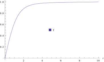
Figure 1: Radial dependence of the profile function of $f(r)$ for $m=1,\leavevmode\nobreak\ \eta=2$ and $\lambda_{1}=0.2$.

The tension (energy per unit length) of these strings is found from the above $\mathcal{H}^{(2)}$. Approximate value of the tension far from the string core is easy to compute if we insert the ansatz at a large distance into the Hamiltonian:

$$T_{\rm PQ}=\mathcal{H}^{(2)}\simeq\int d^{2}x\hbox{\rm Tr}|\partial_{i}\Phi|^{2}\sim 2\pi\times 2\eta^{2}\times m^{2}\log\rho.$$ (24)

We may notice that energy is logarithmically divergent and energy depends on the square of winding number $m^{2}$. The energy stored inside of the core is estimated as of order $\eta^{2}$, to which the scalar potential contributes, and can be neglected at a large distance. It is always energetically favorable to decay higher winding number string into lower winding strings. Since an Alice axion strings have $m=1/2$ as seen later, so an Abelian axion string with $m=1$ decays into two Alice axion strings.

IV.2 Alice axion strings

The Alice axion string is a kind of topological string which changes the sign of electric charge of a probe particle with an original gauge symmetry after one encirclement around the string. In our case, the generator of the unbroken $U(1)_{H}$ changes its sign with the $SU(2)_{H}$ after one rotation. This is because a particle charged under the $U(1)_{H}$ is affected by the broken $SU(2)_{H}$ flux inside the Alice string. To understand this better, let us first consider the field value rotating around an Alice axion string, which depends on the azimuthal angle at a large distance $\rho$,

$$\Phi(\rho,\theta) \sim\eta e^{i\frac{\theta}{2}}\left(\begin{array}[]{ccc}0&e^{i\frac{\theta}{2}}\\ e^{-i\frac{\theta}{2}}&0\end{array}\right)\equiv e^{i\frac{\theta}{2}}\Omega(\theta)\Phi(\rho,0)\Omega^{-1}(\theta),$$ (27)

$$A_{i} \sim-\frac{1}{2g}\frac{\epsilon_{ij}x^{j}}{\rho^{2}}\tau^{3}\leavevmode\nobreak\ (i,j=1,2),\leavevmode\nobreak\ A_{0}=A_{3}=0.$$ (28)

Here, $x^{2}+y^{2}=r^{2},\leavevmode\nobreak\$ $\Phi(\rho,0)=2\eta\tau^{1}=\langle\Phi\rangle$ and the holonomy $\Omega(\theta)$ rotating the $\Phi(\rho,0)$ by $\theta$ can be defined by the broken $SU(2)_{H}$ gauge field:

$$\Omega(\theta)=Pe^{ig\int_{0}^{\theta}{\bf A\cdot dl}}=e^{i\frac{\theta}{2}\tau^{3}}\in SU(2)_{H},$$ (29)

where we used $\partial_{i}\theta=-{\epsilon_{ij}x^{j}}/{r^{2}}$. It is easy to compute the (non-Abelian) flux in the broken $SU(2)_{H}$ trapped inside the string:

$${\rm Flux}=\oint{\bf A\cdot dl}=\frac{\pi}{g}\tau^{3}$$ (30)

Ths $SU(2)$ holonomy can also be $\Omega(\theta)=e^{i\frac{\theta}{2}\tau^{2}}$ or more generally $\Omega(\theta)=e^{i\frac{\theta}{2}\hat{n}}$ with $\hat{n}=\sin\alpha\tau^{2}+\cos\alpha\tau^{3}=e^{i\alpha\tau^{1}}\tau^{3}e^{-i\alpha\tau^{1}}$. Correspondingly, the flux is along $\hat{n}$. The presence of $\alpha$ can be understood as follows. The unbroken symmetry $U(1)_{H}$ of the vacuum is generated by $\tau_{1}$. However, this $U(1)_{H}$ acts on the Alice string solution with a parameter $\alpha$. Namely, the Alice string configuration spontaneously breaks $U(1)_{H}$ symmetry of the vacuum, implying the appearance of a Nambu-Goldstone mode in the vicinity of the Alice string. Therefore, $\alpha$ parametrizes a continuous family of the Alice string solution of the same energy, and is a $U(1)$ modulus of the Alice string Chatterjee:2017hya .

While $\langle\Phi\rangle$ in Eq. (13) is invariant under the $U(1)_{H}$ with $\tau^{1}$, $\Phi(\rho,\theta)$ in Eq. (27) is not invariant under such unbroken elements in Eq. (14) because the unbroken transformation for $\Phi(\rho,\theta)$ becomes angle dependent. The $U(1)_{H}$ generator must be changed by the holonomies with the gauge field when it goes around the Alice string as

$$Q_{\theta}=\Omega(\theta)Q_{0}\Omega(\theta)^{-1}.$$ (31)

Here $Q_{0}\propto\tau^{1},$ thus transformations with $Q_{\theta}$ make $\Phi(\rho,\theta)$ invariant as $e^{i\beta Q_{\theta}}\Phi(\rho,\theta)e^{-i\beta Q_{\theta}}=\Phi(\rho,\theta)$, where $\beta$ is a transformation parameter. After encircling a full loop around the Alice string, we find that $\Omega(2\pi)=e^{i\pi\tau^{3}}\in\mathbb{Z}_{2}\subset H$, hence the unbroken generator becomes

$$Q_{2\pi}=-Q_{0}.$$ (32)

This is nothing but the most characteristic property of the Alice string; the charge of a charged particle flips its sign when it encircles around an Alice string.

To find a solution of the Alice axion string, we shall consider an axisymmetric ansatz as

$$\Phi(r,\theta)=\eta\left(\begin{array}[]{ccc}0&f_{1}(r)e^{i\theta}\\ f_{2}(r)&0\end{array}\right),\qquad A_{i}=-\frac{1}{2g}\frac{\epsilon_{ij}x^{j}}{r^{2}}a(r)\tau^{3}\leavevmode\nobreak\ (i,j=1,2),\leavevmode\nobreak\ A_{0}=A_{3}=0.$$ (35)

where $f_{1,2}(r)$ and $a(r)$ are profile functions of the scalar fields and gauge field with the boundary condition that $f_{1}(0)=f_{2}(0)=0,\leavevmode\nobreak\ f_{1}(\rho)=f_{2}(\rho)=1,\leavevmode\nobreak\ a(0)=0,\leavevmode\nobreak\ a(\rho)=1$. After inserting the above ansatz, two dimensional integration of the static Hamiltonian density can be expressed as

$$\mathcal{H}^{(2)} = \int d^{2}x\left[\frac{1}{2}\hbox{\rm Tr}F_{ij}^{2}++\hbox{\rm Tr}|D_{i}\Phi|^{2}+V(\Phi)\right]$$ (36)

$$= 2\pi\int rdr\bigg{[}\eta^{2}\bigg{\{}f_{1}^{\prime 2}+f_{2}^{\prime 2}+\frac{f_{1}^{2}}{r^{2}}\left(1-\frac{a}{2}\right)^{2}+\frac{f_{2}^{2}}{r^{2}}\frac{a^{2}}{4}+\frac{\eta^{2}\lambda_{1}}{2}(f_{1}^{2}+f_{2}^{2}-2)^{2}+\eta^{2}\lambda_{2}(f_{1}^{2}-f_{2}^{2})^{2}\bigg{\}}+\frac{1}{8g^{2}}\frac{a^{\prime 2}}{r^{2}}\bigg{]}.$$ (37)

As in the Abelian string case, the equations of motion of the profile functions read

$$-\frac{1}{r}\frac{d}{dr}\left(r\frac{d}{dr}f_{1}(r)\right)+\frac{1}{r^{2}}\left(1-\frac{a}{2}\right)^{2}f_{1}(r)+\lambda_{1}\eta^{2}(f_{1}(r)^{2}+f_{2}(r)^{2}-2)f_{1}(r)+2\eta^{2}\lambda_{2}(f_{1}^{2}-f_{2}^{2})f_{1}(r)=0,$$ (38)

$$-\frac{1}{r}\frac{d}{dr}\left(r\frac{d}{dr}f_{2}(r)\right)+\frac{1}{r^{2}}\frac{a^{2}}{4}f_{2}(r)+\lambda_{1}\eta^{2}(f_{1}(r)^{2}+f_{2}(r)^{2}-2)f_{2}(r)-2\eta^{2}\lambda_{2}(f_{1}^{2}-f_{2}^{2})f_{2}(r)=0,$$ (39)

$$-r\frac{d}{dr}\left(\frac{1}{r}\frac{d}{dr}a(r)\right)+4g^{2}\eta^{2}f_{1}(r)^{2}\left(1-\frac{a}{2}\right)+2g^{2}\eta^{2}f_{2}(r)^{2}a(r)=0.$$ (40)

The profile functions are solved numerically for several values of $\lambda_{1}$ and $\lambda_{2}$, and plotted in Fig. 2. It is noted that in the equation of motion for $f_{2}$ the potential contribution can vanish if $\lambda_{1}=2\lambda_{2}$ is taken.

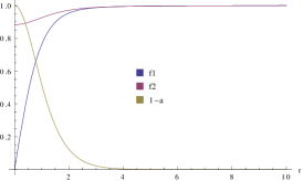
(a)  

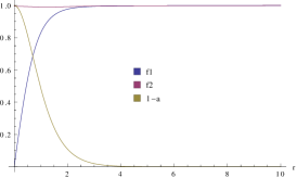
(b)  

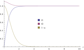
(c)  

Figure 2: Radial dependence of the profile functions of $f_{1}(r),\leavevmode\nobreak\ f_{2}(r)$ and $a(r)$ for $g=0.5$ and $\eta=2$. The remaining parameters are chosen as: (a) $\lambda_{1}=0.2$ and $\lambda_{2}=0.2$ ($\frac{\lambda_{1}}{\lambda_{2}}=1<2$), (b) $\lambda_{1}=0.4$ and $\lambda_{2}=0.2$ ($\frac{\lambda_{1}}{\lambda_{2}}=2$), and (c) $\lambda_{1}=0.6$ and $\lambda_{2}=0.2$ ($\frac{\lambda_{1}}{\lambda_{2}}=3>2$. This is used also in the Sec. V.

The tension far from the string core can be approximately computed with the ansatz at a large distance $\rho$ in Eq. (27):

$$T_{\rm Alice}=\mathcal{H}^{(2)}\simeq\int d^{2}x\hbox{\rm Tr}|\mathcal{D}_{i}\Phi|^{2}\simeq\frac{\pi}{2}\times 2\eta^{2}\log\rho.$$ (41)

It should be noted that the energy of Alice axion string is also logarithmically divergent and the same as that of the Abelian axion string with $m=1/2$ in Eq. (24). Here there would be contribution from $SU(2)$ magnetic field $\frac{1}{2}\hbox{\rm Tr}F_{ij}^{2}$, however that we have neglected due to the logarithmic divergence of the leading term and the energy stored inside the core of the Alice string is estimated as of order $\eta^{2}$, to which fluxes and the scalar potential contribute. As mentioned in the previous subsection, an Abelian axion string (with $m=1$) can decay into two Alice axion strings (with $m=1/2$), since the energy of the Abelian strings gets lower by the decay: $1^{2}>(1/2)^{2}+(1/2)^{2}=1/2$ in the $m=1$ string tension unit, whereas the winding number is conserved. The remaining $1/2$ energy is thought to be converted to axions at the decay, and they will contribute to a fraction of the final abundance of the axion.

IV.3 The decay of an Abelian axion string to two Alice axion strings

In this subsection, we try to understand the decay of the Abelian axion string to the Alice axion strings. As seen above, the tension for the Abelian string is different from the Alice strings by a factor 4. So the Abelian string (with $m=1$) is always energetically favorable to decay into two Alice strings (with $m=1/2$) with the conserved winding number. These two Alice axion strings produced by the decay must have opposite flux direction, since the parent Abelian axion string contains no flux and a field configuration at a large distance does not change through the decay. The configuration of $\Phi$ at an angle $\theta$ and a large distance $\rho$, which is far from the string core, can be in general written by

$$\Phi(\rho,\theta) = h_{0}h\langle\Phi\rangle h^{\dagger},\quad\Omega=\{(h_{0},h)|\leavevmode\nobreak\ h_{0}\in U(1)_{\rm PQ},\leavevmode\nobreak\ h=Pe^{ig\int^{\theta}_{0}{\bf A\cdot dl}}\in SU(2)_{H}\},$$ (42)

$$\Phi(\rho,2\pi) = \Phi(\rho,0)=\langle\Phi\rangle=2\eta\tau^{1},$$ (43)

where $\Omega=\Omega(\theta)$ is a path dependent rotation matrix with two entries around the strings in the axisymmetric case. For an Abelian string, the gauge field is vanishing, whereas for an Alice string with the positive flux the gauge field is given by the ansatz in the previous subsection. For a full loop we have $\Omega(2\pi)=(h_{0}(2\pi),\leavevmode\nobreak\ h(2\pi))\in H$ of $O(2)$, where $h(2\pi)=Pe^{ig\oint{\bf A\cdot dl}}$. For a rotation around the Abelian axion strings by $\theta$, $\Omega^{0}(\theta)=(e^{i\theta},\leavevmode\nobreak\ 1)$ and $\Omega^{0}(2\pi)=(1,1)\in H$, where zero denotes for one rotation around the Abelian axion string. For a rotation by $\theta$ around a single axisymmetric Alice axion string with a positive flux, $\Omega^{+}(\theta)=(e^{i\frac{\theta}{2}},e^{i\frac{\theta}{2}\tau^{3}})$ and $\Omega^{+}(2\pi)=\{-1,i\sigma^{3}\}\in H$. This is similar to $\Omega^{-}$ for the Alice string with a negative flux: $\Omega^{-}(\theta)=(e^{i\frac{\theta}{2}},e^{-i\frac{\theta}{2}\tau^{3}})$ and $\Omega^{-}(2\pi)=\{-1,-i\sigma^{3}\}\in H$.

Now let us understand what happens at the decay of the Abelian axion string to two Alice axion strings. Just at the time when a single Abelian axion string is split into two Alice strings, the boundary condition remains unchanged because it is understood with $\Omega$. To show it, we draw a loop $C$ around the Abelian axion string before splitting. In this case, the $\Omega$ is given by $\Omega^{0}(C)=(1,1)$. Just after the splitting, we divide the loop in two parts as $C=C_{1}+C_{2}$ and we close the loops by connecting the points $a$ and $b$ by the path $R$ as shown in the Fig. 3 In this case we have

$$\Omega^{-}(C_{1}+R) = (h_{0}(C_{1}+R)=e^{i\pi},\leavevmode\nobreak\ h(C_{1}+R)=Pe^{ig\oint_{C_{1}+R}{\bf A\cdot dl}})$$ (44)

$$\Omega^{+}(C_{2}-R) = (h_{0}(C_{2}-R)=e^{i\pi},\leavevmode\nobreak\ h(C_{2}-R)=Pe^{ig\oint_{C_{2}-R}{\bf A\cdot dl}}).$$ (45)

So we find

$$\Omega^{0}(C)=\Omega^{+}(C_{2}-R)\Omega^{-}(C_{1}+R)=(1,Pe^{ig\oint_{C}{\bf A\cdot dl}}=1).$$ (46)

This shows that field configurations at a large distances do not change, while the splitting takes place.

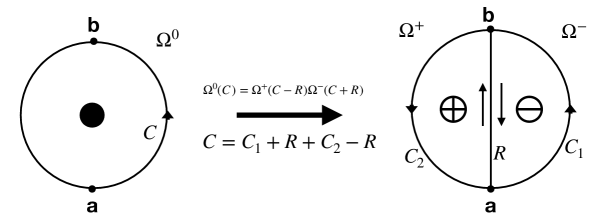
Figure 3: Loops around the strings. Left: A loop $C$ around the Abelian axion string. Right: A loop $C$ is decomposed to $C_{1}+R$ and $C_{2}-R$, where the former is a loop around the Alice axion string with the negative flux and the latter is a loop around the Alice string with the positive flux.

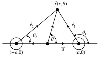
Figure 4: A configuration of two Alice axion strings. One Alice string with the negative flux is at $(a,0)$ in the $x$-$y$ plane, whereas another with the positive flux is at $(-a,0)$. $|\vec{r}_{1,2}|$ are the distance vectors from the two Alice strings from the point ${\vec{r}}=(r,\theta)$, and $\theta_{1,2}$ are the angles around them.

To estimate the force between two Alice axion strings, we take a large distance approximation, following Ref. Nakano:2007dr for the same problem in the context of non-Abelian strings in dense QCD Eto:2013hoa . Suppose that there exist two heavy Alice strings, which do not move, on the $x$-axis in the $x-y$ plane at a large distance of $2a$ apart as shown in Fig. 4. So the fields are approximately written as

$$\Phi\sim e^{i(\theta_{1}+\theta_{2})}Pe^{ig\int_{0}^{\theta}{\bf{\bf A\cdot dl}}}\langle\Phi\rangle Pe^{-ig\int_{0}^{\theta}{\bf A\cdot dl}},\leavevmode\nobreak\ A_{i}(x,y)\sim A_{i}^{(+)}(x,y)+A_{i}^{(-)}(x,y)\leavevmode\nobreak\ (i=1,2),\leavevmode\nobreak\ A_{0}=A_{3}=0,$$ (47)

where $A_{i}^{(+)}$ ($A_{i}^{(-)}$) is the gauge fields relevant to the positive flux (negative flux) inside the Alice string in the absence of another string with the negative flux (positive flux). So the energy at large distances can be approximately written by

$$\mathcal{E}\simeq\int d^{2}x\hbox{\rm Tr}|\mathcal{D}_{i}\Phi|^{2}\simeq 2\eta^{2}\int d^{2}x\left[\partial_{i}(\theta_{1}+\theta_{2})\right]^{2}+\cdots$$ (48)

Here we neglected small contribution from the gauge field. It is found also that $\int d^{2}x\left[(\partial_{i}\theta_{1})^{2}+(\partial_{i}\theta_{2})^{2}\right]\simeq 2\times T_{\rm Alice}$. So the interaction energy can be expressed as

$$\mathcal{E}_{int} \simeq 4\eta^{2}\int d^{2}x\partial_{i}\theta_{1}\partial_{i}\theta_{2}+\cdots$$ (49)

$$=4\eta^{2}\cdot 2\pi\int drr\left[\frac{r^{2}-a^{2}}{r^{4}+a^{4}-2r^{2}a^{2}\cos 2\theta}\right]$$

$$\simeq 4\pi\eta^{2}\log\left(\frac{\rho^{2}+a^{2}}{a^{2}}\right).$$

Here we used $\partial_{i}\theta=-\epsilon_{ij}x^{j}/r^{2}$ and this is similar to $\theta_{1,2}$. The force between two Alice axion strings is found to be repulsive:

$$\text{Force}=-\frac{1}{2}\frac{\partial\mathcal{E}_{int}}{\partial a}\simeq+\frac{4\pi\eta^{2}}{a}\leavevmode\nobreak\ \leavevmode\nobreak\ \leavevmode\nobreak\ {\rm for}\leavevmode\nobreak\ \rho\rightarrow\infty.$$ (50)

This repulsive force is mediated by the light QCD axion at a large distance apart. This is analogous to a Coulomb force between particles with the same charge in two spatial dimension. Hence, the distance between two Alice axion strings would increase with time and it is confirmed from numerical calculation. However, note that our simulation is done in a relaxation method but not in a real time dynamics.

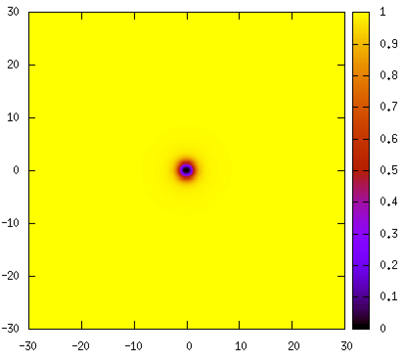
(a)  

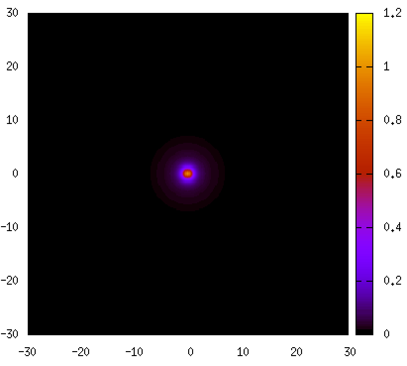
(b)  

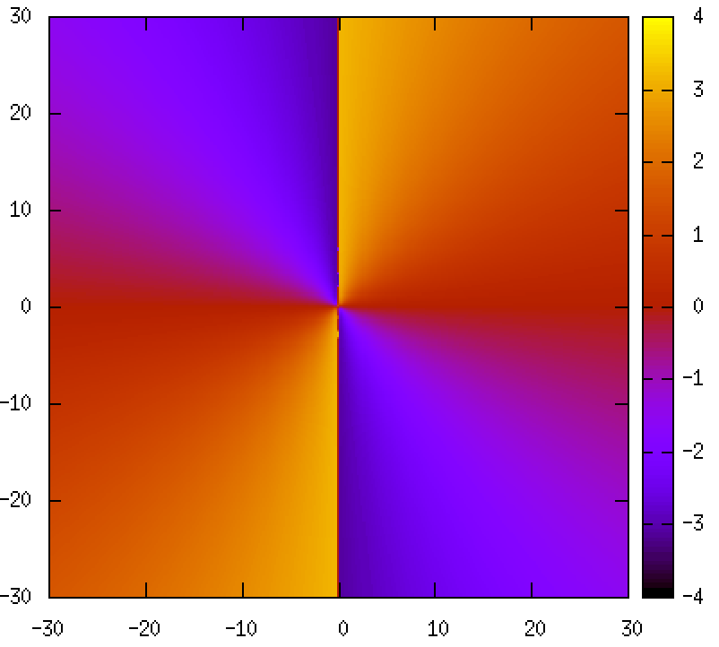
(c)  

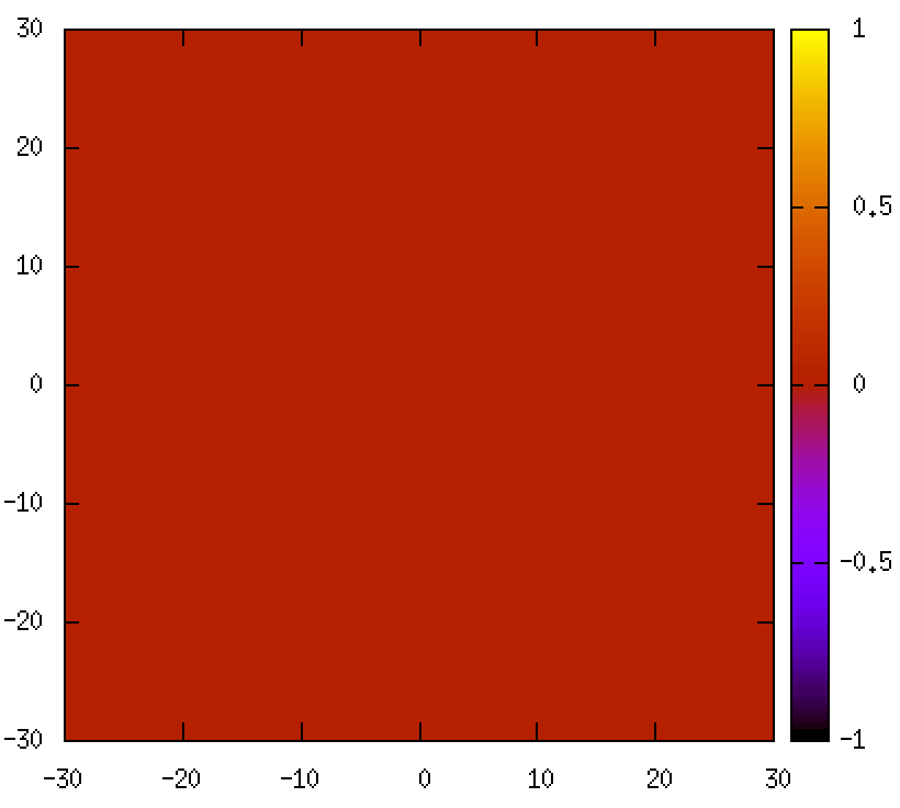
(d)  

Figure 5: Figures of an Abelian axion string before the splitting for $g=1,\leavevmode\nobreak\ \eta=0.5,\leavevmode\nobreak\ \lambda_{1}=2.0$ and $\lambda_{2}=0.25$. They show $2\hbox{\rm Tr}(({\Phi}^{2})^{\dagger}\Phi^{2})$, the static energy, the phase $\Im\log\hbox{\rm Tr}\Phi^{2}(x,y)$ and non-Abelian magnetic field $F_{12}^{3}(x,y)$ (with a gauge fixing) from left to right. It is easy to check there is a phase jump by $2\pi$ around each string solution.

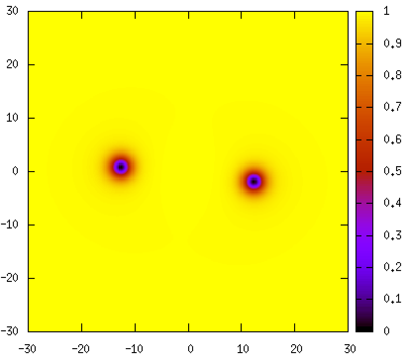
(a)  

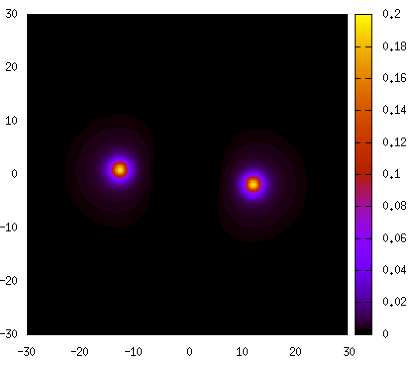
(b)  

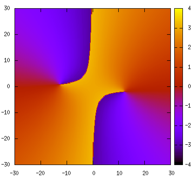
(c)  

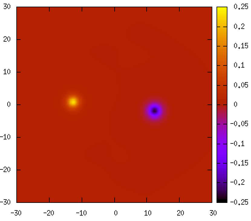
(d)  

Figure 6: Similar figures of two Alice axion strings after the decay from the parent Abelian axion string.

For numerical solutions, we used $500\times 500$ lattice with lattice spacing $0.2$. We relaxed the system in $1000000$ time steps with each time step $\Delta t=10^{-3}$. The other parameters are taken as $g=1,\leavevmode\nobreak\ \eta=0.5,\leavevmode\nobreak\ \lambda_{1}=2.0$ and $\lambda_{2}=0.25$.

V Domain wall-string composite

So far we discussed two types of axion strings and decay of a Abelian axion string to two Alice axion strings. In this section, we study configuration of domain walls attached to the Abelian axion string or to the Alice string. The former situation involving the Abelian strings may be realized at the chiral phase transition through the Kibble-Zurek mechanism Kibble:1976sj ; Zurek:1985qw : At the chiral phase transition, two kinds of domain walls may be created elsewhere. If these domain walls collide, they can be glued along an Abelian axion string. The latter situation involving the Alice strings will always take place in our case. To find the domain walls attached to an Abelian axion string, we start with $\mu\neq 0$ in the potential of Eq. (20). The static Hamiltonian density (in $A_{0}=0$ gauge) is given by

$$\mathcal{H} = \frac{1}{2}\hbox{\rm Tr}F_{ij}^{2}++\hbox{\rm Tr}|D_{i}\Phi|^{2}+\frac{\lambda_{1}}{2}\left(\hbox{\rm Tr}\Phi^{\dagger}\Phi-2\eta^{2}\right)^{2}+\frac{\lambda_{2}}{2}\hbox{\rm Tr}\big{(}[\Phi,\Phi^{\dagger}]^{2}\big{)}$$ (51)

$$+\mu\left({\rm Det}\Phi+{\rm Det}\Phi^{\dagger}\right)+{\rm const.}$$

We shall first discuss vacua in the presence of Abelian axion strings and the Alice axion strings and focus a parameter region, in which $2\eta^{2}\lambda_{1}>\mu$ is satisfied, for $V_{\rm DW}$ not to affect $\langle\Phi\rangle$ significantly. This is natural for axion domain wall since $\mu$ is expected to be of order $m_{a}^{2}$.

V.1 Abelian axion string-domain wall composite

First let us consider an Abelian axion strings. Below we show that a single Abelian axion string is attatched by two domain walls. To understand a situation in the presence of the walls attached to the Abelian axion string, we shall consider an approximate ansatz of the string at a large distance as

$$\Phi\sim 2\eta e^{i\alpha}\tau^{1},\leavevmode\nobreak\ \leavevmode\nobreak\ \leavevmode\nobreak\ A_{\mu}=0.$$ (52)

Substituting the above ansatz into Eq. (51), we find

$$\mathcal{H}\sim 2\eta^{2}\left[\left(\partial_{i}\alpha\right)^{2}+\mu\left(1-\cos 2\alpha\right)\right].$$ (53)

The potential in the above Hamiltonian is nothing but the potential of Eq. (19) wth $\alpha=a/2\eta$. As noted already, $\alpha$ sweeps full circle ($0\leq\alpha\leq 2\pi$) around the axion string, however, the potential shows that system have two vacua at $\alpha=0$ or $\pi$ and this would create two domain walls attached to the Abelian axion string: $N_{\rm DW}=2$. $\alpha$ would be almost zero or $\pi$ everywhere however changes at the place where domain walls are created. In other words, there are two different domain walls: One is connecting the vacuum at $\alpha=0$ and that at $\alpha=\pi$. Another is doing the vacuum at $\alpha=\pi$ and that at $\alpha=2\pi\equiv 0$. We call them DW1 and DW2 respectively. The whole configuration can be regarded as a junction of these two domain walls (DW1 and DW2), whose junction line is nothing but an Abelian axion string. Fig. 7 shows a full numerical simulation of such a configuration, obtained by the relaxation method. We used larger lattice of $700\times 700$ points with lattice spacing $0.2$. We have taken $g=1,\leavevmode\nobreak\ \mu=1.4,\leavevmode\nobreak\ \eta=0.5,\leavevmode\nobreak\ \lambda_{1}=2.0$ and $\lambda_{2}=0.25$ for our computation of domain wall-string composites. Here, we put a large friction around a string to prevent this configuration to decay, as described below.

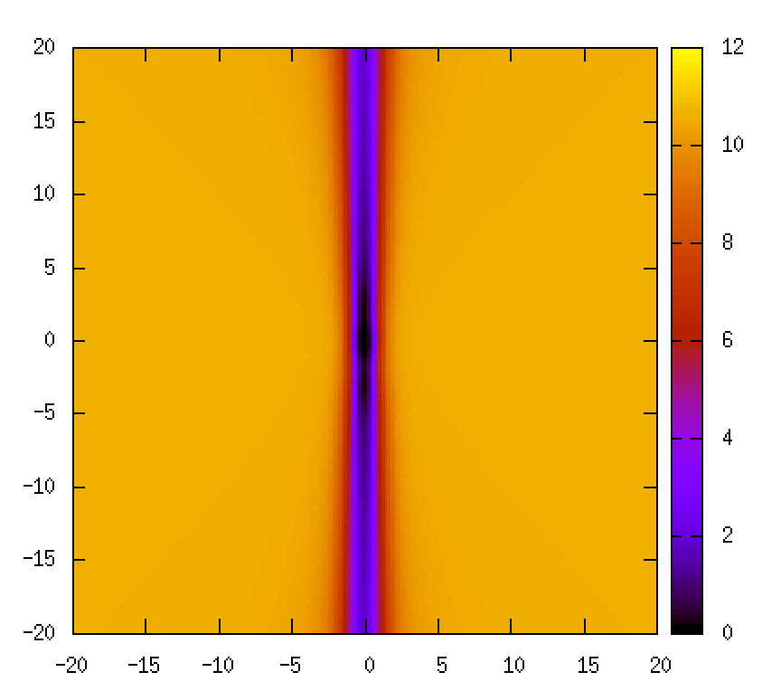
(a)  

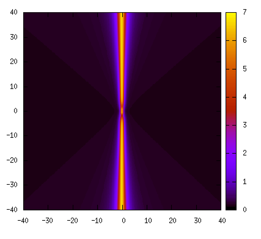
(b)  

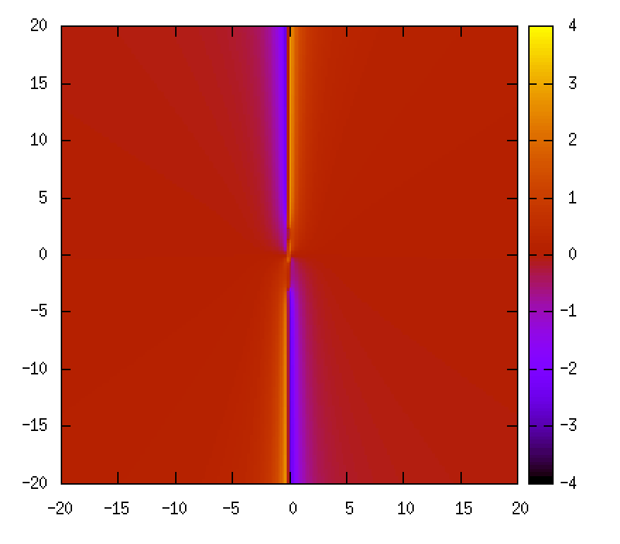
(c)  

Figure 7: Figures of two domain walls attached to one Abelian axion string before the decay for $\mu=1.4,\leavevmode\nobreak\ g=1,\leavevmode\nobreak\ \eta=0.5,\leavevmode\nobreak\ \lambda_{1}=2.0$ and $\lambda_{2}=0.25$. The string exists at the center in each figures. They show: (a) $2\hbox{\rm Tr}(({\Phi}^{2})^{\dagger}\Phi^{2})$, (b) the energy density, and (c) the phase $2\alpha$. It is noted that the $\alpha$ changes by $\pi$ at crossing the domain wall.

V.2 Alice axion string-domain wall composite

In this subsection we discuss the formation of domain walls in the presence of two Alice strings produced via the decay of the parent Abelian axion string. To understand behavior of the walls, we similarly start with field configurations at a large distance as

$$\Phi\sim\eta\left(\begin{array}[]{ccc}0&e^{i\alpha}\\ 1&0\\ \end{array}\right),\qquad A_{i}\sim-\frac{1}{2g}\frac{\epsilon_{ij}x^{j}}{r^{2}}\tau^{3}\leavevmode\nobreak\ (i,j=1,2),\leavevmode\nobreak\ A_{0}=A_{3}=0.$$ (56)

With this ansatz, the static Hamiltonian density in Eq. (51) reads

$$\mathcal{H}\sim\eta^{2}\left[\frac{1}{2}(\partial_{i}\alpha)^{2}+2\mu\left(1-\cos\alpha\right)\right].$$ (57)

Here we may check the difference from Eq. (53). In this case, the vacuum is still at $\alpha=0$ (or $2\pi$) whereas the field range is given by $0\leq\alpha\leq 2\pi$. As a result, there will exist only one domain wall attached to one Alice axion string. This is a similar to the vacuum with $N_{\rm DW}=1$. The model is also identical to the sine-Gordon model in two dimension and a domain wall solution along the $x$-axis interpolating between the two vacua can be written as $\alpha=4\tan^{-1}e^{\pm\sqrt{2\mu}x}$.

For $\mu\neq 0$ in computation, when an Abelian axion string attached by two domain walls is initially created and decays into two Alice axion strings, each domain walls remains attached to Alice strings as shown in the Fig. 8. For numerical calculations, the relaxation method is used and the same parameters are chosen as before.

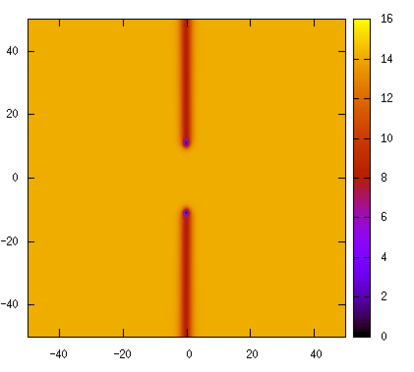
(a)  

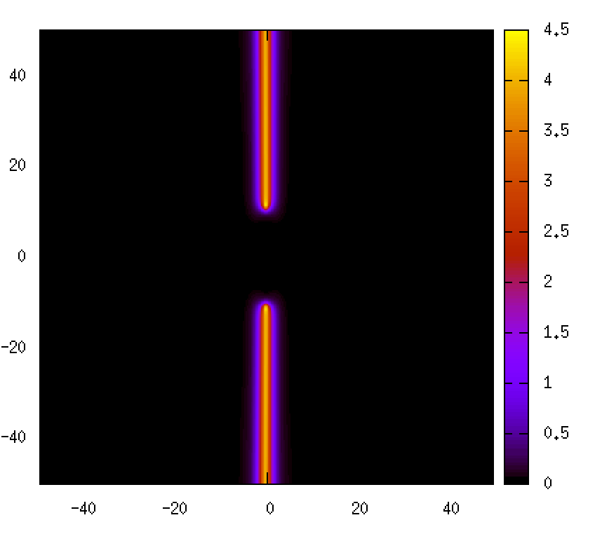
(b)  

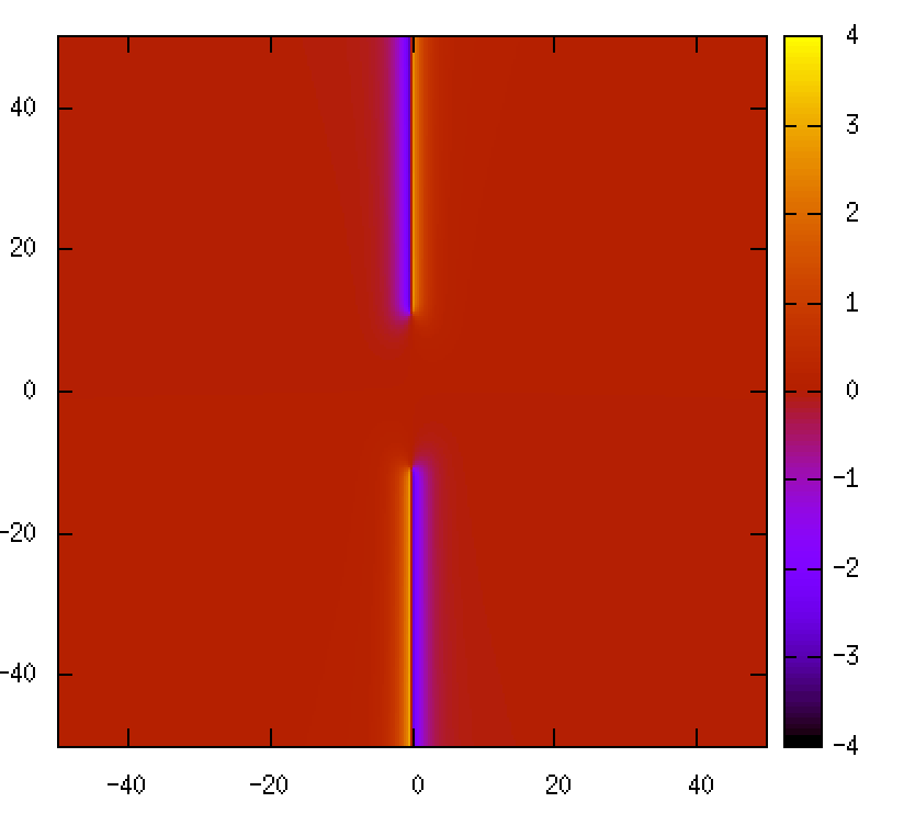
(c)  

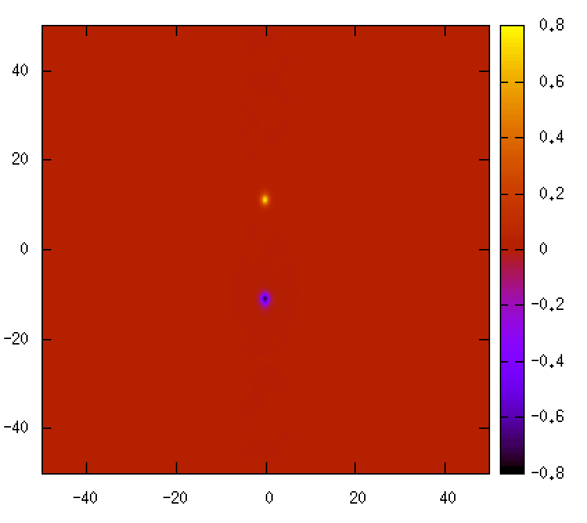
(d)  

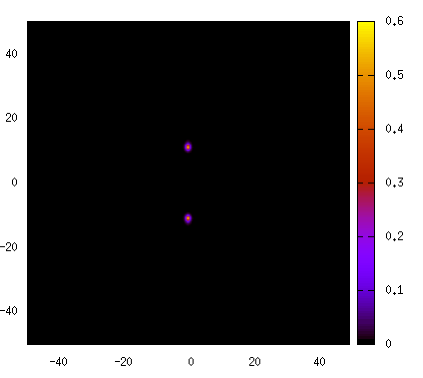
(e)  

Figure 8: Figures of two domain walls attached to two each Alice axion strings after the decay of the parent Abelian axion string for $\mu=1.4\leavevmode\nobreak\ g=1\leavevmode\nobreak\ \eta=0.5,\leavevmode\nobreak\ \lambda_{1}=2.0$ and $\lambda_{2}=0.25$. They show: (a) $2\hbox{\rm Tr}(({\Phi}^{2})^{\dagger}\Phi^{2})$, (b) energy density, (c) the phase $\alpha$, (d) non-Abelian magnetic field $F_{12}^{3}(x,y)$, (e) the magnitude of the magnetic fields $\sum_{\alpha}{F^{\alpha}}^{2}_{12}$. It is noted that $\alpha$ changes by $2\pi$ at crossing the domain wall.

There exist two kinds of the Alice axion strings when one focuses on Eq. (27). One has the non-Abelian flux parallel to the orientation defined by the $U(1)_{\rm PQ}$: $e^{i\theta/2}\Omega=e^{i\theta/2}e^{i\theta\tau^{3}/2}$, where $e^{i\theta/2}\in U(1)_{\rm PQ}$. Another has the flux opposite to the orientation: $e^{i\theta/2}\Omega=e^{i\theta/2}e^{-i\theta\tau^{3}/2}$ (with a modulus parameter of $\pi$). We call these strings Alice1 and Alice2 respectively. To flip the sign simultaneously by $\theta\to-\theta$ gives the same configuration because this is to see the same string in different ways: the string seen from a positive $z$ coordinate or from a negative $z$ coordinate. So, Alice2 with $e^{i\theta/2}e^{-i\theta\tau^{3}/2}$ is physically equivalent to that with $e^{-i\theta/2}e^{i\theta\tau^{3}/2}$. Factors of $e^{\pm i\theta/2}$ in $U(1)_{\rm PQ}$ (with the same $\Omega=e^{i\theta\tau^{3}/2}$) imply the way to approach domain walls in the axion space. After one rotation around the Alice1 with $0\leq\theta/2\leq\pi$, one meets DW1. Further, with $\Omega(2\pi)=e^{i\pi\tau^{3}}\in{\mathbb{Z}}_{2}\subset H$, the vacuum is smoothly connected. At the chiral phase transition, like in $N_{\rm DW}=1$ case, a single Alice1 is attached by a single DW1, whereas a single Alice2 is attached by a single DW2. See Fig. 9.

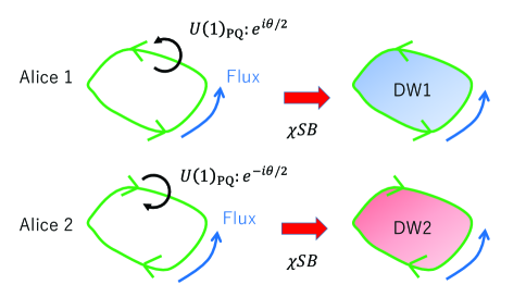
Figure 9: A schematic figure for Alice strings attached by domain walls. There exist also two kinds of Alice string depending on the orientation and the flux. At the chiral phase transition, DW1 is attached to Alice1 whereas DW2 is attached to Alice2.

In the actual cosmological history, once an Abelian string is created after the PQ symmetry breaking, it will quickly decay into two Alice strings in the presence of the repulsive force between them. Then domain walls, which are created after the chiral symmetry breaking, attach to Alice strings, and they shrink to a point owing to the wall tension like in the $N_{\rm DW}=1$ case. Even if an Abelian sting attached by two domain walls is created at the chiral phase transition by the Kibble-Zurek mechanism, the Abelian string can be split into two Alice strings in the presence of the wall tension. Then, one Alice string is attached by one wall and each of the walls similarly shrinks to a point by the tension. See Fig. 10.

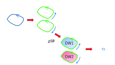
(a)  

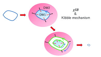
(b)  

Figure 10: Schematic figures for decay of Abelian axion string into two Alice strings attached by domain walls. (a) An Abelian axion string can quickly decay into two Alice strings in the early universe. (b) Even if an Abelian string survives at the chiral phase transition, it can be split into two Alice strings attached by domain walls in the presence of domain wall tension. In both cases, each of the walls shrinks to a point by the tension finally.

VI Conclusion and discussions

Axion is an attractive candidate of dark matter, while stable networks composed by stable strings and walls may be created after the breakdown of $U(1)_{\rm PQ}$ and ${\mathbb{Z}}_{N_{\rm DW}}$ embedded in $U(1)_{\rm PQ}$. They can cause cosmological disasters since the energy density of them can finally dominate the that of the universe. The Lazarides-Shafi mechanism is one of solutions to the domain wall problem. We have studied this mechanism in detail based on a recently proposed model Sato:2018nqy , showing dynamics of axion strings and walls. Even if Abelian axion strings are formed in the early universe, each of them is split into multiple Alice axion strings due to a repulsive force between the Alice strings even without domain wall. When domain walls are formed as the universe cools down, a single Alice string is attached by a single wall because a vacuum is connected by a non-Abelian rotation without changing energy. Such walls do not form stable networks since they collapse by the tension of the walls, emitting axions. Even if domain walls attached to the Abelian axion strings is created by the Kibble-Zurek mechanism at the chiral phase transition, the Abelian string can be split into Alice strings and one domain wall is attached to one Alice axion strings. Such walls can shrink to a point owing to the wall tension like in $N_{\rm DW}=1$ case.

Several discussions are addressed here. The model of Ref. Sato:2018nqy was also proposed as a model for a monopole dark matter. A monopole in the conventional Alice theory ($SO(3)$ gauge theory with scalar fields of the fiveplet) admitting Alice strings was studied in Refs. Shankar:1976un ; Bais:2002ae ; Striet:2003na ; Benson:2004ue . In particular, a monopole is not spherical and decays into a twisted Alice ring depending on choice of parameters Bais:2002ae ; Striet:2003na . It would be interesting to study if the same would happen in our case. In fact, it is known that a global analog (global monopole) shows this property Ruostekoski:2003qx . A dyon with an electric $U(1)_{H}$ charge may be realized as a vorton, namely a persistent electric current flows along a ring. Dyons can be dark matter if their (mini) electric charge, which may be obtained via a kinetic mixing between $U(1)_{H}$ and electromagnetism, is below experimental bounds. It is also worth to point out that the conventional monopole charge of $\pi_{2}$ is not well defined in the presence of an Alice string, because a monopole becomes an anti-monopole when it encircles around an Alice string, as a dual of electric charge encircling around the Alice string. Instead of using the usual homotopy group $\pi_{2}$, a monopole charge must be defined in terms of the Abe homotopy Kobayashi:2011xb .

There can exist infinitely long (Abelian) strings produced after the PQ breaking. In such cases, the scaling solution is found to be violated by a logarithmic growth of the string scaling parameter in time Gorghetto:2018myk ; Kawasaki:2018bzv . It might be hard for wide walls attached to long strings to shrink to a point, hence simulations for them may also be altered. When two Abelian cosmic strings collide, they reconnect each other, which is important process for cosmic strings to reduce their number. Alice strings have $U(1)$ moduli corresponding to fluxes, and so it is unclear if they can reconnect. As this regards, two non-Abelian strings with non-Abelian fluxes were shown to always reconnect Eto:2006db , and so it would be true for Alice strings. Further, a nature of reconnection among Alice strings may be different from that among Abelian strings due to a force existing among Alice strings, so the number of long Alice strings could differ from that of long Abelian string. The number of long Alice strings would be significant to a solution to the domain wall problem. In any cases, the axion abundance needs to be correctly estimated and may be modified from Eq. (9). Thus, an allowed region for the axion decay constant may be altered. If there is no allowed region, the PQ symmetry breaking might be required to take place before or during inflation, and constraint on insocurvature may be important then.

In future observations, gravitational waves produced by the decay of strings and walls may be detected, depending on axion model Saikawa:2017hiv ; Higaki:2016jjh . That can be an important signal to verify the presence of axion dark matter produced by the topological objects.

If topological objects appear in dark matter models, it is necessary to study the nature of the objects in detail, for precise estimation of dark matter.

References

- (1) C. A. Baker et al., “An Improved experimental limit on the electric dipole moment of the neutron,” Phys. Rev. Lett. 97, 131801 (2006) [hep-ex/0602020].
- (2) R. D. Peccei and H. R. Quinn, “CP Conservation in the Presence of Instantons,” Phys. Rev. Lett. 38, 1440 (1977).
- (3) R. D. Peccei and H. R. Quinn, “Constraints Imposed by CP Conservation in the Presence of Instantons,” Phys. Rev. D 16, 1791 (1977).
- (4) S. Weinberg, “A New Light Boson?,” Phys. Rev. Lett. 40, 223 (1978).
- (5) G. G. Raffelt, “Astrophysical axion bounds,” Lect. Notes Phys. 741, 51 (2008) [hep-ph/0611350].
- (6) J. Preskill, M. B. Wise and F. Wilczek, “Cosmology of the Invisible Axion,” Phys. Lett. B 120, 127 (1983). [Phys. Lett. 120B, 127 (1983)].
- (7) L. F. Abbott and P. Sikivie, “A Cosmological Bound on the Invisible Axion,” Phys. Lett. B 120, 133 (1983). [Phys. Lett. 120B, 133 (1983)].
- (8) M. Dine and W. Fischler, “The Not So Harmless Axion,” Phys. Lett. B 120, 137 (1983) [Phys. Lett. 120B, 137 (1983)].
- (9) J. E. Kim and G. Carosi, “Axions and the Strong CP Problem,” Rev. Mod. Phys. 82, 557 (2010) [arXiv:0807.3125 [hep-ph]]; references therein.
- (10) M. Kawasaki and K. Nakayama, “Axions: Theory and Cosmological Role,” Ann. Rev. Nucl. Part. Sci. 63, 69 (2013) [arXiv:1301.1123 [hep-ph]]; references therein.
- (11) T. W. B. Kibble, G. Lazarides and Q. Shafi, “Walls Bounded by Strings,” Phys. Rev. D 26, 435 (1982).
- (12) A. Vilenkin and A. E. Everett, “Cosmic Strings and Domain Walls in Models with Goldstone and PseudoGoldstone Bosons,” Phys. Rev. Lett. 48, 1867 (1982).
- (13) A. E. Everett and A. Vilenkin, “Left-right Symmetric Theories and Vacuum Domain Walls and Strings,” Nucl. Phys. B 207, 43 (1982).
- (14) Y. B. Zeldovich, I. Y. Kobzarev and L. B. Okun, “Cosmological Consequences of the Spontaneous Breakdown of Discrete Symmetry,” Zh. Eksp. Teor. Fiz. 67, 3 (1974) [Sov. Phys. JETP 40, 1 (1974)].
- (15) J. Preskill and A. Vilenkin, “Decay of metastable topological defects,” Phys. Rev. D 47, 2324 (1993) [hep-ph/9209210].
- (16) Y. Akrami et al. [Planck Collaboration], “Planck 2018 results. X. Constraints on inflation,” arXiv:1807.06211 [astro-ph.CO].
- (17) M. Kawasaki, K. Saikawa and T. Sekiguchi, “Axion dark matter from topological defects,” Phys. Rev. D 91, no. 6, 065014 (2015) [arXiv:1412.0789 [hep-ph]].
- (18) V. B. .Klaer and G. D. .Moore, “The dark-matter axion mass,” JCAP 1711, no. 11, 049 (2017) [arXiv:1708.07521 [hep-ph]].
- (19) A. Vilenkin, “Gravitational Field of Vacuum Domain Walls and Strings,” Phys. Rev. D 23, 852 (1981); P. Sikivie, “Of Axions, Domain Walls and the Early Universe,” Phys. Rev. Lett. 48, 1156 (1982); G. B. Gelmini, M. Gleiser and E. W. Kolb, “Cosmology of Biased Discrete Symmetry Breaking,” Phys. Rev. D 39, 1558 (1989).
- (20) G. Lazarides and Q. Shafi, “Axion Models with No Domain Wall Problem,” Phys. Lett. 115B, 21 (1982).
- (21) M. Kawasaki, F. Takahashi and M. Yamada, “Suppressing the QCD Axion Abundance by Hidden Monopoles,” Phys. Lett. B 753, 677 (2016) [arXiv:1511.05030 [hep-ph]].
- (22) R. Sato, F. Takahashi and M. Yamada, “Unified Origin of Axion and Monopole Dark Matter, and Solution to the Domain-wall Problem,” Phys. Rev. D 98, no. 4, 043535 (2018) [arXiv:1805.10533 [hep-ph]].
- (23) M. Kawasaki, M. Yamada and T. T. Yanagida, “Observable dark radiation from a cosmologically safe QCD axion,” Phys. Rev. D 91, no. 12, 125018 (2015) [arXiv:1504.04126 [hep-ph]].
- (24) A. A. Abrikosov, “On the Magnetic properties of superconductors of the second group,” Sov. Phys. JETP 5, 1174 (1957) [Zh. Eksp. Teor. Fiz. 32, 1442 (1957)].
- (25) H. B. Nielsen and P. Olesen, “Vortex Line Models for Dual Strings,” Nucl. Phys. B 61, 45 (1973).
- (26) M. B. Hindmarsh and T. W. B. Kibble, “Cosmic strings,” Rept. Prog. Phys. 58, 477 (1995) [hep-ph/9411342].
- (27) A. Vilenkin and E. P. S. Shellard, “Cosmic Strings and Other Topological Defects,” (Cambridge Monographs on Mathematical Physics), Cambridge University Press (July 31, 2000).
- (28) A. S. Schwarz, “Field Theories With No Local Conservation Of The Electric Charge,” Nucl. Phys. B 208, 141 (1982).
- (29) J. E. Kiskis, “Disconnected Gauge Groups and the Global Violation of Charge Conservation,” Phys. Rev. D 17, 3196 (1978).
- (30) M. G. Alford, K. Benson, S. R. Coleman, J. March-Russell and F. Wilczek, “The Interactions and Excitations of Nonabelian Vortices,” Phys. Rev. Lett. 64 (1990) 1632 [Erratum-ibid. 65 (1990) 668].
- (31) M. G. Alford, K. Benson, S. R. Coleman, J. March-Russell and F. Wilczek, “Zeromodes of nonabelian vortices,” Nucl. Phys. B 349 (1991) 414.
- (32) M. G. Alford, K. M. Lee, J. March-Russell and J. Preskill, “Quantum field theory of nonAbelian strings and vortices,” Nucl. Phys. B 384 (1992) 251.
- (33) J. Preskill and L. M. Krauss, “Local Discrete Symmetry and Quantum Mechanical Hair,” Nucl. Phys. B 341, 50 (1990).
- (34) M. Bucher and A. Goldhaber, “SO(10) Cosmic strings and SU(3)-color Cheshire charge,” Phys. Rev. D 49 (1994) 4167 [hep-ph/9310262].
- (35) M. Bucher, H. K. Lo and J. Preskill, “Topological approach to Alice electrodynamics,” Nucl. Phys. B 386, 3 (1992) [hep-th/9112039].
- (36) H. K. Lo and J. Preskill, “NonAbelian vortices and nonAbelian statistics,” Phys. Rev. D 48 (1993) 4821 [hep-th/9306006].
- (37) J. Striet and F. A. Bais, “Simple models with Alice fluxes,” Phys. Lett. B 497, 172 (2000) [hep-th/0010236].
- (38) E. B. Bogomolny, “Stability of Classical Solutions,” Sov. J. Nucl. Phys. 24, 449 (1976) [Yad. Fiz. 24, 861 (1976)].
- (39) M. K. Prasad and C. M. Sommerfield, “An Exact Classical Solution for the ’t Hooft Monopole and the Julia-Zee Dyon,” Phys. Rev. Lett. 35, 760 (1975).
- (40) C. Chatterjee and M. Nitta, “BPS Alice strings,” JHEP 1709, 046 (2017) [arXiv:1703.08971 [hep-th]].
- (41) C. Chatterjee and M. Nitta, “The effective action of a BPS Alice string,” Eur. Phys. J. C 77, no. 11, 809 (2017) [arXiv:1706.10212 [hep-th]].
- (42) U. Leonhardt and G. E. Volovik, “How to create Alice string (half quantum vortex) in a vector Bose-Einstein condensate,” Pisma Zh. Eksp. Teor. Fiz. 72, 66 (2000) [JETP Lett. 72, 46 (2000)] [cond-mat/0003428].
- (43) J. Ruostekoski and J. R. Anglin, “Monopole core instability and Alice rings in spinor Bose-Einstein condensates,” Phys. Rev. Lett. 91, 190402 (2003) Erratum: [Phys. Rev. Lett. 97, 069902 (2006)] [cond-mat/0307651].
- (44) S. Kobayashi, M. Kobayashi, Y. Kawaguchi, M. Nitta and M. Ueda, “Abe homotopy classification of topological excitations under the topological influence of vortices,” Nucl. Phys. B 856, 577 (2012) [arXiv:1110.1478 [math-ph]].
- (45) Y. Kawaguchi and M. Ueda, “Spinor Bose-Einstein condensates,” Phys. Rept. 520, 253 (2012).
- (46) T. W. B. Kibble, “Topology of Cosmic Domains and Strings,” J. Phys. A 9, 1387 (1976).
- (47) W. H. Zurek, “Cosmological Experiments in Superfluid Helium?,” Nature 317, 505 (1985).
- (48) J. E. Kim, “Weak Interaction Singlet and Strong CP Invariance,” Phys. Rev. Lett. 43, 103 (1979).
- (49) M. A. Shifman, A. I. Vainshtein and V. I. Zakharov, “Can Confinement Ensure Natural CP Invariance of Strong Interactions?,” Nucl. Phys. B 166, 493 (1980).
- (50) M. Dine, W. Fischler and M. Srednicki, “A Simple Solution to the Strong CP Problem with a Harmless Axion,” Phys. Lett. 104B, 199 (1981).
- (51) A. R. Zhitnitsky, “On Possible Suppression of the Axion Hadron Interactions. (In Russian),” Sov. J. Nucl. Phys. 31, 260 (1980) [Yad. Fiz. 31, 497 (1980)].
- (52) T. Hiramatsu, M. Kawasaki, K. Saikawa and T. Sekiguchi, “Axion cosmology with long-lived domain walls,” JCAP 1301, 001 (2013) [arXiv:1207.3166 [hep-ph]].
- (53) E. Witten, “Dyons of Charge e theta/2 pi,” Phys. Lett. B 86, 283 (1979) [Phys. Lett. 86B, 283 (1979)].
- (54) E. Del Nobile, M. Nardecchia and P. Panci, “Millicharge or Decay: A Critical Take on Minimal Dark Matter,” JCAP 1604, no. 04, 048 (2016) [arXiv:1512.05353 [hep-ph]].
- (55) D. S. Akerib et al. [LUX Collaboration], “Results from a search for dark matter in the complete LUX exposure,” Phys. Rev. Lett. 118, no. 2, 021303 (2017) [arXiv:1608.07648 [astro-ph.CO]].
- (56) W. Fischler and J. Preskill, “Dyon - Axion Dynamics,” Phys. Lett. 125B, 165 (1983).
- (57) Y. Nomura, S. Rajendran and F. Sanches, “Axion Isocurvature and Magnetic Monopoles,” Phys. Rev. Lett. 116, no. 14, 141803 (2016) [arXiv:1511.06347 [hep-ph]].
- (58) M. Kawasaki, F. Takahashi and M. Yamada, “Adiabatic suppression of the axion abundance and isocurvature due to coupling to hidden monopoles,” JHEP 1801, 053 (2018) [arXiv:1708.06047 [hep-ph]].
- (59) E. Nakano, M. Nitta and T. Matsuura, “Non-Abelian strings in high density QCD: Zero modes and interactions,” Phys. Rev. D 78, 045002 (2008) [arXiv:0708.4096 [hep-ph]].
- (60) M. Eto, Y. Hirono, M. Nitta and S. Yasui, “Vortices and Other Topological Solitons in Dense Quark Matter,” PTEP 2014, no. 1, 012D01 (2014) [arXiv:1308.1535 [hep-ph]].
- (61) R. Shankar, “More SO(3) monopoles” Phys. Rev. D 14, 1107 (1976).
- (62) F. A. Bais and J. Striet, “On a core instability of ’t Hooft-Polyakov monopoles,” Phys. Lett. B 540, 319 (2002) [hep-th/0205152].
- (63) J. Striet and F. A. Bais, “More on core instabilities of magnetic monopoles,” JHEP 0306, 022 (2003) [hep-th/0304189].
- (64) K. M. Benson and T. Imbo, “Topologically Alice strings and monopoles,” Phys. Rev. D 70, 025005 (2004) [hep-th/0407001].
- (65) M. Gorghetto, E. Hardy and G. Villadoro, JHEP 1807, 151 (2018) doi:10.1007/JHEP07(2018)151 [arXiv:1806.04677 [hep-ph]].
- (66) M. Kawasaki, T. Sekiguchi, M. Yamaguchi and J. Yokoyama, PTEP 2018, no. 9, 091E01 (2018) doi:10.1093/ptep/pty098 [arXiv:1806.05566 [hep-ph]].
- (67) M. Eto, K. Hashimoto, G. Marmorini, M. Nitta, K. Ohashi and W. Vinci, “Universal Reconnection of Non-Abelian Cosmic Strings,” Phys. Rev. Lett. 98, 091602 (2007) [hep-th/0609214].
- (68) For a recent review see e.g. K. Saikawa, “A review of gravitational waves from cosmic domain walls,” Universe 3, no. 2, 40 (2017) [arXiv:1703.02576 [hep-ph]].
- (69) T. Higaki, K. S. Jeong, N. Kitajima, T. Sekiguchi and F. Takahashi, “Topological Defects and nano-Hz Gravitational Waves in Aligned Axion Models,” JHEP 1608, 044 (2016)