Roberge-Weiss periodicity, canonical sector and modified Polyakov-loop

Abstract

To obtain deeper understanding of QCD properties at finite temperature, we consider the Fourier decomposition of the grand-canonical partition function based on the canonical ensemble method via the imaginary chemical potential. Expectation values are, then, represented by summation over each canonical sector. We point out that the modified Polyakov-loop can play an important role in the canonical ensemble; for example, the Polyakov-loop paradox which is known in the canonical ensemble method can be evaded by considering the quantity. In addition, based on the periodicity issue of the modified Polyakov-loop at finite imaginary chemical potential, we can construct the systematic way to compute the dual quark condensate which has strong unclearness in its foundation in the presence of dynamical quarks so far.

I Introduction

Extensive studies for exploring the phase diagram of quantum chromodynamics (QCD) have been done at finite temperature ($T$) and real chemical potential ($\mu_{\mathrm{R}}$). In the study of QCD, the lattice QCD simulation is a powerful and gauge invariant approach to investigate its non-perturbative nature. Lattice QCD simulation, however, has the well-known sign problem at finite $\mu_{\mathrm{R}}$; see Ref. de Forcrand (2009) as an example. Therefore, several approaches have been proposed so far such as the Taylor expansion method Allton et al. (2005); *Gavai:2008zr, the reweighting method Fodor and Katz (2002a); *Fodor:2001pe; *Fodor:2004nz; *Fodor:2002km, the analytic continuation method de Forcrand and Philipsen (2002); *deForcrand:2003vyj; *DElia:2002tig; *DElia:2004ani; *Chen:2004tb, the canonical ensemble method Hasenfratz and Toussaint (1992); *Alexandru:2005ix; Kratochvila and de Forcrand (2006); *deForcrand:2006ec; *Li:2010qf and so on. However, the application range of these approaches are still limited in the small $\mu_{\mathrm{R}}/T$ region.

In comparison, the imaginary chemical potential ($\mu_{\mathrm{I}}$) region does not have the sign problem and thus we can perform the lattice QCD simulation, exactly. Interestingly, the $\mu_{\mathrm{I}}$ region can play a crucial role to understand QCD properties at finite $\mu_{\mathrm{R}}$ via the analytic continuation method and the canonical ensemble method. Thus, this region is very useful. In addition, it has been recently proposed that the structure of QCD at finite $\mu_{\mathrm{I}}$ may be related with the confinement-deconfinement transition Kashiwa and Ohnishi (2015); *Kashiwa:2016vrl; *Kashiwa:2017yvy based on the analogy of the topological order at $T=0$ Wen (1990); Sato (2008). Because of these reasons, it is interesting and important to know detailed properties of QCD at finite $\mu_{\mathrm{I}}$.

The canonical ensemble method which is strongly related with the imaginary chemical potential region is the interesting and well known method: there is the mathematical reason that the canonical partition functions can be constructed from the grand-canonical partition function with $\mu_{\mathrm{I}}$ via the Fourier transformation and the fugacity expansion Roberge and Weiss (1986). This approach has been applied to the lattice QCD simulation and successfully performed in moderate and high temperature regions. The canonical ensemble method, however, has the Polyakov-loop paradox Kratochvila and de Forcrand (2006). This paradox induces the problem that the Polyakov loop cannot be used as the order parameter/indicator in the canonical ensemble method because the Polyakov-loop becomes always zero at any $T$.

It is easily to understand that the Polyakov-loop paradox is induced from the fact that the Polyakov loop does not have the Roberge-Weiss (RW) periodicity; for example see Fig. 1. In other words, the Polyakov loop is no longer good quantity to characterize the imaginary chemical potential region. Thus, we employ the modified Polyakov-loop in this article; it is known as the RW periodic quantity and can describe the RW transition nature. We show that the Polyakov-loop paradox can be evaded by using the modified Polyakov-loop in this study; we can reproduce the Polyakov loop via the canonical ensemble method. In addition to resolve the Polyakov-loop paradox, we can clarify the foundation of the dual quark condensate Bilgici et al. (2008) from the RW periodicity issue of the modified Polyakov-loop; this quantity has been proposed as the order parameter or the indicator of the deconfinement transition, but it has strong unclearness in its determination so far.

This paper is organized as follows. In the next section, we summarize important properties of QCD at finite imaginary chemical potential. Section III shows the possible QCD effective model which reproduces the QCD properties at finite imaginary chemical potential; we need the model to demonstrate our observation. The Polyakov-loop paradox in the canonical ensemble method is explained in Sec. IV. In Sec. V, we discuss how the Polyakov-loop paradox can be evaded by using the modified Polyakov-loop. We show the theoretical foundation of the dual quark condensate from the RW periodicity of the modified Polyakov-loop in Sec. VI. Section VII is devoted to summary.

II Structure of QCD at finite imaginary chemical potential

The QCD grand-canonical partition function (${\cal Z}_{\mathrm{GC}}$) has following properties at finite $\theta:=\mu_{\mathrm{I}}/T$;

1. The Roberge-Weiss (RW) periodicity

The imaginary chemical potential can be transformed into the quark temporal boundary condition and then the $\mathbb{Z}_{3}$-transformation which induces the $\mathbb{Z}_{3}$ factor to the quark field can be also absorbed into the boundary condition. Consequently, we have

$${\cal Z}_{\mathrm{GC}}(T,\theta)={\cal Z}_{\mathrm{GC}}\Bigl{(}T,\theta+\frac{2\pi k}{N_{\mathrm{C}}}\Bigr{)},$$ (1)

where $N_{\mathrm{c}}$ is the number of color and $k\in\mathbb{N}$. This periodicity of ${\cal Z}_{\mathrm{GC}}$ causes the $2\pi/N_{\mathrm{c}}$ periodicity of several thermodynamic quantities such as the pressure, the entropy and the quark number density. This special $2\pi/N_{\mathrm{c}}$ periodicity is so called the RW periodicity Roberge and Weiss (1986).

2. Existence of $\mathbb{Z}_{N_{\mathrm{c}}}$ images

It is well known that there are $\mathbb{Z}_{N_{\mathrm{c}}}$ images at high $T$. These images are corresponding to minimum of the thermodynamic potential and one of them becomes the global minima in certain range of $\theta$. However, different minima which is the local minima of the thermodynamic potential in the certain range of $\theta$ can become the global minima when the $\theta$ range is changed. The images can be characterized by the phase of the Polyakov loop ($\phi$): For example,

Non-trivial

$\phi=2\pi/3$ for $\theta=[-\pi,-\pi/3]$

Trivial

$\phi=0$ for $\theta=[-\pi/3,\pi/3]$

Non-trivial

$\phi=-2\pi/3$ for $\theta=[\pi/3,\pi]$

are all possible $\mathbb{Z}_{N_{\mathrm{c}}}$ images for $N_{\mathrm{c}}=3$ at sufficiently high $T$. The realistic system exists with the trivial $\mathbb{Z}_{N_{\mathrm{c}}}$ image where $\Phi\in\mathbb{R}$. These images, however, vanished at low $T$ and then only one minimum appears, but the RW periodicity still exists.

3. The RW transition

The origin of the RW periodicity at low and high $T$ are perfectly different. At low $T$, hadronic contributions are quite strong and then the RW periodicity is induced by the baryonic fugacity, $e^{\pm 3i\theta}$, and then there is no singularity along $\theta$ direction. On the other hand, the quark fugacity, $e^{\pm i(gA_{4}/T+\theta)}$, jumps into the game at high $T$ where $g$ is the gauge coupling constant. In this case, the RW periodicity is induced via the $\mathbb{Z}_{3}$ images; i.e. the global minima of the thermodynamic potential switches to another minimum when we across $\theta=(2k-1)\pi/3$ and then the singularities arise in thermodynamic quantities. This singularity induces the phase transition along $\theta$ direction and it is so called the RW transition Roberge and Weiss (1986).

4. RW endpoint

The RW endpoint is the endpoint of the first-order RW transition. Since the singularities appear when the RW transition happen, there should be the endpoint at certain $T$ which is usually denoted by $T_{\mathrm{RW}}$. The order of the endpoint may depend on the number of flavor with physical quark mass; some lattice QCD simulations indicate that the order is first-order and then the RW endpoint is the triple-point in the two- and three-flavor systems de Forcrand and Philipsen (2010); D’Elia and Sanfilippo (2009); Bonati et al. (2011). However, some lattice QCD simulations indicate the second-order RW endpoint even below the physical quark mass in the $2+1$ flavor system Bonati et al. (2016, 2019); Goswami et al. (2018).

Based on these properties, several studies for the confinement-deconfinement transition have been done; the first attempt is Ref. Weiss (1987), some related discussions are show in Refs. Kashiwa and Ohnishi (2015); *Kashiwa:2016vrl; *Kashiwa:2017yvy and this paper. Also, some of them have been used to investigate the correlation between the confinement-deconfinement transition and the chiral phase transition via the state-of-art anomaly matching Kikuchi ; Yonekura (2019); Nishimura and Tanizaki (2019).

III Possible QCD effective model

To demonstrate our observation as shown later, we need the effective model of QCD which reproduces QCD properties at finite $\mu_{\mathrm{I}}$. The Polyakov-loop extended Nambu–Jona-Lasinio (PNJL) model Fukushima (2004) is the famous and promising effective model for this purpose. The PNJL model can approximately describe the deconfinement and chiral phase transitions at the same time by introducing non-perturbative effects through the NJL model and Polyakov-loop effective potential Meisinger et al. (2002); Fukushima (2004); Dumitru et al. (2011); see Ref. Fukushima and Skokov (2017) for details. It should be noted that main results presented in this paper are model independent, qualitatively. We use the effective model to perform the numerical calculations to demonstrate our knowledge.

The Lagrangian density of the two-flavor and three-color PNJL model in the Euclidean space is

$${\cal L} ={\bar{q}}({\ooalign{\hfil/\hfil\crcr$D$}}+m_{0})q$$ (4)

$$-G[({\bar{q}}q)^{2}+({\bar{q}}i\gamma_{5}{\vec{\tau}}q)^{2}]+{\cal V}_{\mathrm{g}}(\Phi,{\bar{\Phi}}),$$ (5)

where $q$ represents the quark field, the covariant derivative is $D_{\nu}=\partial_{\nu}-igA_{\nu}\delta_{\nu 4}$, ${\cal V}_{\mathrm{g}}$ expresses the gluonic contribution and $\Phi$ (${\bar{\Phi}}$) means the Polyakov-loop (its conjugate). The actual form of the effective potential with the mean-field approximation is

$${\cal V}_{\mathrm{PNJL}} ={\cal V}_{\mathrm{f}}+{\cal V}_{\mathrm{g}},$$ (6)

with

$${\cal V}_{\mathrm{f}} =-2N_{\mathrm{f}}\int_{\Lambda}\frac{d^{3}p}{(2\pi)^{3}}\Bigl{[}N_{\mathrm{c}}E_{\bf p}+T\ln\Bigl{(}f^{-}f^{+}\Bigr{)}\Bigr{]}+G\sigma^{2},$$ (7)

where $\Lambda$ is the three-dimensional momentum cutoff. The Fermi-Dirac distribution functions become

$$f^{-} =1+3(\Phi+{\bar{\Phi}}e^{-\beta E_{\bf p}^{-}})e^{-\beta E_{\bf p}^{-}}+e^{-3\beta E_{\bf p}^{-}},~{}~{}~{}~{}$$

$$f^{+} =1+3({\bar{\Phi}}+\Phi e^{-\beta E_{\bf p}^{+}})e^{-\beta E_{\bf p}^{+}}+e^{-3\beta E_{\bf p}^{+}},$$ (8)

where $E^{\mp}_{\bf p}=E_{\bf p}\mp\mu$ and $E_{\bf p}=\sqrt{{\bf p}^{2}+M^{2}}$ with $\mu=(\mu_{\mathrm{R}},\mu_{\mathrm{I}})$ and $M=m_{0}-2G\sigma$. The condensate $\sigma$ is defined as $\sigma\equiv\langle{\bar{q}}q\rangle$. The parameter set used in the NJL part is taken from Ref. Kashiwa et al. (2008).

In this article, we employ the logarithmic Polyakov-loop effective potential Roessner et al. (2007) as the effective model for the gluonic contribution. The functional form is

$$\frac{{\cal V}_{\mathrm{g}}}{T^{4}} =-\frac{1}{2}a(T){\bar{\Phi}}\Phi$$

$$+b(T)\ln\Bigl{[}1-6{\bar{\Phi}}\Phi+4({\bar{\Phi}}^{3}+\Phi^{3})-3({\bar{\Phi}}\Phi)^{2}\Bigr{]},$$ (9)

with

$$a(T) =a_{0}+a_{1}\Bigl{(}\frac{T_{0}}{T}\Bigr{)}+a_{2}\Bigl{(}\frac{T_{0}}{T}\Bigr{)}^{2},$$

$$b(T) =b_{3}\Bigl{(}\frac{T_{0}}{T}\Bigr{)}^{3},$$ (10)

where parameters, $(a_{0},a_{1},a_{2},b_{3})$, are taken from Ref. Roessner et al. (2007). The remaining parameter $T_{0}$ is usually fixed as $270$ MeV which is the critical temperature in the pure gauge limit. In the case of full QCD, $T_{0}$ may be determined to reproduce the pseudo-critical temperature of the deconfinement transition at zero $\mu$. However, we still use $T_{0}=270$ MeV because we are interested in the qualitative behavior in this article. The RW endpoint temperature in the present setting is about $T_{\mathrm{RW}}=254$ MeV. In following discussions, we use the PNJL model with above setting.

IV Canonical ensemble method

In the standard calculation to investigate the QCD phase diagram, we start from the grand-canonical partition function;

$${\cal Z}_{\mathrm{GC}}(T,\mu) =\int[{\cal D}A][{\cal D}{q}][{\cal D}{\bar{q}}]e^{-S_{\mathrm{QCD}}(\mu)},$$ (11)

where $S_{\mathrm{QCD}}$ is the QCD Euclidean action and $A$ means the gluon field. It is well known that we can construct the canonical partition function with fixed real quark number (Q), ${\cal Z}_{\mathrm{C}}(T,Q)$, from the grand-canonical partition function by using $\theta$ Roberge and Weiss (1986); Hasenfratz and Toussaint (1992) as

$${\cal Z}_{\mathrm{C}}(T,Q) =\frac{1}{2\pi}\int_{-\pi}^{\pi}d\theta~{}e^{-iQ\theta}{\cal Z}_{\mathrm{GC}}(T,\theta).$$ (12)

The domain of integration is usually fixed as $\theta=[-\pi,\pi]$. Since the QCD grand-canonical partition function has the RW periodicity, Eq. (12) can be rewritten as

$${\cal Z}_{\mathrm{C}}(T,Q) ={\cal Z}^{Q}_{C}\Bigl{(}T,-\pi,-\frac{\pi}{3}\Bigr{)}+{\cal Z}^{Q}_{C}\Bigl{(}T,-\frac{\pi}{3},\frac{\pi}{3}\Bigr{)}$$

$$+{\cal Z}^{Q}_{C}\Bigl{(}T,\frac{\pi}{3},\pi\Bigr{)},$$ (13)

where

$${\cal Z}^{Q}_{C}(T,a,b) =\frac{1}{2\pi}\int_{a}^{b}d\theta~{}e^{-iQ\theta}{\cal Z}_{\mathrm{GC}}(T,\theta).$$ (14)

Therefore, ${\cal Z}_{\mathrm{C}}(T,Q)$ becomes

$${\cal Z}_{\mathrm{C}} =\Bigl{(}1+e^{i\frac{2\pi Q}{3}}+e^{-i\frac{2\pi Q}{3}}\Bigr{)}{\cal Z}^{Q}_{C}\Bigl{(}T,-\frac{\pi}{3},\frac{\pi}{3}\Bigr{)}$$

$$=\begin{dcases}0\hskip 81.09052ptQ\neq 0~{}\mathrm{mod}~{}3\\ 3{\cal Z}^{Q}_{C}\Bigl{(}T,-\frac{\pi}{3},\frac{\pi}{3}\Bigr{)}\hskip 14.22636ptQ=0~{}\mathrm{mod}~{}3.\\ \end{dcases}$$ (15)

Then, the expectation value of an arbitrary RW periodic operator (${\cal O}$) is given by

$$\langle{\cal O}\rangle_{\mathrm{C}} =\frac{1}{2\pi}\int_{-\pi}^{\pi}d\theta~{}\Bigl{(}\frac{{\mathcal{Z}}_{\mathrm{GC}}}{{\cal Z}_{\mathrm{C}}}\Bigr{)}e^{-iQ\theta}\langle{\cal O}\rangle_{\mathrm{GC}}$$

$$=\begin{dcases}\hskip 8.10913pt\mathrm{undefined~{}or~{}finite}\hskip 22.76228ptQ\neq 0~{}\mathrm{mod}~{}3\\ \hskip 8.5359pt\mathrm{can~{}be~{}nonzero}~{}~{}~{}~{}~{}~{}~{}~{}~{}~{}~{}Q=0~{}\mathrm{mod}~{}3.\\ \end{dcases}$$ (16)

The “undefined” means that we encounter $0/0$ in the calculation, but it can be defined if we remove the factor, $(1+z+z^{2})$ where $z=\exp(2\pi Qi/3)$, by reducing the fractions to a common denominator because the factor appears in both the denominator and the numerator. Below, we follow the latter interpretation; $\langle{\cal O}\rangle_{C}$ with $Q\neq 0~{}\mathrm{mod}~{}3$ are finite. This expression cannot be used for the Polyakov loop because the Polyakov loop is transformed as $e^{2i\pi k/3}\Phi$ under the $\mathbb{Z}_{3}$-transformation. This means that the Polyakov loop does not show the RW periodicity; it can be clearly seen from Fig. 1.

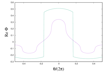
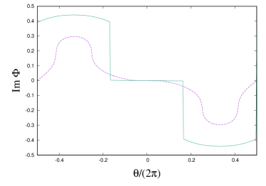
Figure 1: The top and bottom panels show the $\theta$-dependence of the real and imaginary parts of the Polyakov loop, respectively. The dotted and solid lines are results at $T=240$ and $260$ MeV, respectively.

Because of the RW transition, $\mathrm{Re}\,\Phi$ and $\mathrm{Im}\,\Phi$ have the gap at $\theta=(2k-1)\pi/3$ at sufficiently high $T$.

In comparison, the expectation value of the Polyakov loop which is the RW un-periodic operator becomes

$$\langle\Phi\rangle_{\mathrm{C}} =\frac{1}{2\pi}\int_{-\pi}^{\pi}d\theta~{}\Bigl{(}\frac{{\mathcal{Z}}_{\mathrm{GC}}}{{\cal Z}_{\mathrm{C}}}\Bigr{)}e^{-iQ\theta}\langle\Phi\rangle_{\mathrm{GC}}$$

$$=\begin{dcases}\hskip 8.5359pt\mathrm{undefined}~{}~{}~{}~{}~{}Q\neq 0~{}\mathrm{mod}~{}3\\ \hskip 8.5359pt0\hskip 54.06006ptQ=0~{}\mathrm{mod}~{}3.\\ \end{dcases}$$ (17)

Therefore, the Polyakov loop behaves differently comparing with the RW periodic quantities (16). This behavior induces the paradox which is so called the Polyakov-loop paradox; the canonical sectors with the quark number $Q\neq 0~{}\mathrm{mod}~{}3$ become unphysical and thus we must only sum up contributions with $Q=0~{}\mathrm{mod}~{}3$ to avoid the divergence when we calculate $\langle\Phi\rangle$ by using $Z_{\mathrm{C}}$;

$$\langle\Phi\rangle_{\mathrm{GC^{\prime}}} =\sum_{Q=-\infty}^{\infty}e^{Q\mu/T}\Bigl{(}\frac{{\mathcal{Z}}_{\mathrm{C}}}{{\cal Z}_{\mathrm{GC}}}\Bigr{)}\langle\Phi\rangle_{\mathrm{C}}(T,Q)$$

$$\to\sum_{B=-\infty}^{\infty}e^{3B\mu/T}\Bigl{(}\frac{{\mathcal{Z}}_{\mathrm{C}}}{{\cal Z}_{\mathrm{GC}}}\Bigr{)}\langle\Phi\rangle_{\mathrm{C}}(T,3B).$$ (18)

Then, we always obtain

$$\langle\Phi\rangle_{\mathrm{GC^{\prime}}}=0,$$ (19)

from the canonical ensemble method at any $T$. This is so called the Polyakov loop paradox Kratochvila and de Forcrand (2006).

V Roles of Modified Polyakov-loop

To evade the Polyakov-loop paradox, we here consider the modified Polyakov-loop Sakai et al. (2008) defined as

$$\Psi =e^{i\theta}\Phi.$$ (20)

On the RW transition lines at $\theta=(2k-1)\pi/3$, the imaginary part of the quark number density and the modified Polyakov-loop can have the nonzero value. This transition can be understood from the spontaneous shift symmetry ($({\mathbb{Z}_{2})}_{\mathrm{shift}}$) breaking. The $(\mathbb{Z}_{2})_{\mathrm{shift}}$ symmetry at $\theta=(2\pi-1)/\mathrm{N_{c}}$ is the invariance under the transformation associated with the time reversal (${\cal T}$) or the charge conjugation (${\cal C}$) and $\mathbb{Z}_{\mathrm{N_{c}}}$ transformations via the semidirect product Kashiwa et al. (2013); Shimizu and Yonekura (2018); Kikuchi ; Nishimura and Tanizaki (2019);

$$\mathbb{Z}_{2}\rtimes\mathbb{Z}_{\mathrm{N_{c}}}.$$ (21)

The Polyakov loop under the $({\mathbb{Z}_{2})}_{\mathrm{shift}}$ transformation just at $\theta=\lim_{\epsilon\to 0}(\pi/3-\epsilon)$ is

$$\Phi =e^{-i\pi/3}|\Phi|\xrightarrow[~{}~{}\mathbb{Z}_{3}~{}]{}e^{i\pi/3}|\Phi|\xrightarrow[~{}~{}\mathbb{Z}_{2}~{}]{}\Phi~{}~{}\mathrm{for~{}low~{}}T,$$

$$\Phi =|\Phi|\xrightarrow[~{}~{}\mathbb{Z}_{3}~{}]{}e^{-i2\pi/3}|\Phi|\xrightarrow[~{}~{}\mathbb{Z}_{2}~{}]{}\times\hskip 11.38109pt\Phi~{}~{}\hskip 15.649pt\mathrm{for~{}high~{}}T,$$ (22)

but the imaginary part of the modified Polyakov-loop is transformed as

$$\mathrm{Im}~{}\Psi\xrightarrow[({\mathbb{Z}_{2})}_{\mathrm{shift}}]{}\times\hskip 22.76219pt\mathrm{Im}~{}\Psi~{}~{}\hskip 11.38109pt\mathrm{for~{}all~{}}T,$$ (23)

where $A\xrightarrow[~{}~{}{B}~{}~{}]{}\times\hskip 14.22636ptC$ means that $A$ is not transformed to $C$ by using $B$ transformation. Therefore, we can use $\mathrm{Im}\,\Psi$ as the order parameter to detect the spontaneous $({\mathbb{Z}_{2})}_{\mathrm{shift}}$ symmetry breaking. In the case of $SU(2)$, we have the stick symmetry Ishiyama et al. (2010) and then the Polyakov loop can be used to detect it exactly at $\theta=(2k-1)\pi/2$.

The modified Polyakov-loop is known as the RW periodic quantity and thus it can become nonzero value within the canonical ensemble method; we define it as

$$\langle\Psi\rangle_{\mathrm{C}}(Q,T)$$

$$=\frac{1}{2\pi}\int_{-\pi}^{\pi}d\theta~{}\Bigl{(}\frac{{\mathcal{Z}}_{\mathrm{GC}}}{{\cal Z}_{\mathrm{C}}}\Bigr{)}e^{-iQ\theta}\langle\Psi\rangle_{\mathrm{GC}}$$

$$=\begin{dcases}\hskip 8.5359pt\mathrm{finite}\hskip 70.5627ptQ\neq 0~{}\mathrm{mod}~{}3\\ \hskip 8.5359pt\mathrm{can~{}be~{}nonzero}~{}~{}~{}~{}~{}~{}~{}~{}Q=0~{}\mathrm{mod}~{}3.\\ \end{dcases}$$ (24)

The modified Polyakov-loop can reflect the Polyakov-loop dynamics in QCD and thus we can evade the Polyakov-loop paradox by using it; see the next section for more details. Actually, we can rewrite the Polyakov-loop appearing in the partition function into the modified Polyakov-loop because $e^{i\theta}$ which can be interpreted as the fermion boundary condition should be coupled with the temporal component of the link variable and thus all dynamical variables in QCD can be RW periodic; it can be clearly seen in PNJL model in Eq. (16) of Ref. Sakai et al. (2008).

VI Equivalent representation

At $\mu_{\mathrm{R}}=0$, we can simply evaluate the expectation values via the following representation denoted by $\langle\cdots\rangle_{\mathrm{C}}^{\prime}$;

$$\langle{\cal O}\rangle_{\mathrm{C}}^{\prime}(T,Q) \equiv\frac{1}{2\pi}\int_{-\pi}^{\pi}d\theta~{}e^{-iQ\theta}\langle{\cal O}\rangle_{\mathrm{GC}},$$ (25)

because we can reach the expression

$$\sum_{Q=-\infty}^{\infty}\langle{\cal O}\rangle^{\prime}_{\mathrm{C}}=\sum_{Q=-\infty}^{\infty}\Bigl{(}\frac{{\cal Z}_{\mathrm{C}}}{{\cal Z}_{\mathrm{GC}}(\theta=0)}\Bigr{)}\langle{\cal O}\rangle_{\mathrm{C}},$$ (26)

from following procedure: This expression is obtained by using the relation

$$\frac{1}{2\pi}\sum_{Q=-\infty}^{\infty}e^{-iQ\theta} =F(\theta),~{}~{}~{}~{}-\pi\leq\theta\leq\pi,$$ (27)

where $F(\theta)$ is the $2\pi$-periodic delta function

$$F(\theta) =\sum_{k}\delta(\theta+2\pi k),$$ (28)

here the $2\pi$-periodicity of the Matsubara frequency is the origin of the periodicity of $F(\theta)$. Then, the following relation is mathematically true;

$$\langle\Phi\rangle^{\prime}_{\mathrm{C}}(T,Q)$$

$$=\begin{dcases}\hskip 8.5359pt0\hskip 82.51282ptQ+1\neq 0~{}\mathrm{mod}~{}3\\ \hskip 8.5359pt\mathrm{can~{}be~{}nonzero}\hskip 21.33955ptQ+1=0~{}\mathrm{mod}~{}3.\\ \end{dcases}$$ (29)

Since the partition function itself is difficult to treat in the effective model with the mean-field approximation because we should take the thermodynamic limit, Eq. (25) is convenient for our purpose. With Eq. (25), we can qualitatively discuss the canonical ensemble because it shares same properties with $\langle{\cal O}\rangle_{\mathrm{C}}$; for example, the expectation value of the Polyakov-loop in the grand-canonical ensemble has contributions from the sector with $Q~{}\neq 0~{}\mathrm{mod}~{}3$ Kratochvila and de Forcrand (2006).

To go beyond the Polyakov-loop paradox, we consider the Fourier transformation of the modified Polyakov-loop;

$$\langle\Psi\rangle^{\prime}(T,Q) =\frac{1}{2\pi}\int_{-\pi}^{\pi}d\theta~{}e^{-iQ\theta}\langle\Psi\rangle_{\mathrm{GC}}$$

$$=\frac{1}{2\pi}\int_{-\pi}^{\pi}d\theta~{}e^{-i(Q-1)\theta}\langle\Phi\rangle_{\mathrm{GC}}.$$ (30)

The most important point in this article is that we can have $\langle\Psi\rangle=\langle\Phi\rangle$ at $\mu_{\mathrm{R}}=0$ by shifting $(Q-1)$ to $Q^{\prime}$ as

$$\langle\Phi\rangle_{\mathrm{GC}}=\sum_{Q=-\infty}^{\infty}\langle\Phi\rangle^{\prime}(T,Q) =\sum_{Q^{\prime}=-\infty}^{\infty}\langle\Psi\rangle^{\prime}(T,Q)=\langle\Psi\rangle_{\mathrm{GC}},$$ (31)

when $Q$ and $Q^{\prime}$ run from $-\infty$ to $\infty$. This relation means that we can evade the Polyakov-loop paradox by using the modified Polyakov-loop when we calculate the Polyakov-loop with the canonical ensemble because $\Psi$ is the RW periodic quantity. There may be the difference between $\langle\Phi\rangle$ and $\langle\Psi\rangle$ in the finite size system where maximum $|Q|$ and $|Q^{\prime}|$ exist. It should be noted that we cannot exactly discuss $\langle\Phi\rangle_{\mathrm{GC}}$ at $\mu_{\mathrm{R}}\neq 0$ via $\langle\Psi\rangle_{\mathrm{C}}^{\prime}$ because we use Eq. (27) with the fugacity expansion, but it is possible to compute $\langle\Phi\rangle_{\mathrm{GC}}$ via $\langle\Psi\rangle_{\mathrm{C}}$, in principle.

In addition, above fact indicates that we can restrict the domain of integral to $-\pi/3\sim\pi/3$ from $-\pi\sim\pi$ in the Fourier transformation because its domain of integral can be restricted in one period;

$$\Sigma^{(n)}: =\frac{1}{2\pi}\int_{-\pi/3}^{\pi/3}d\theta~{}e^{-in\theta}\langle\sigma\rangle_{\mathrm{GC}},$$ (32)

$$\Psi^{(n)}: =\frac{1}{2\pi}\int_{-\pi/3}^{\pi/3}d\theta~{}e^{-in\theta}\langle\Psi\rangle_{\mathrm{GC}},$$

$$=\frac{1}{2\pi}\int_{-\pi/3}^{\pi/3}d\theta~{}e^{-i(n-1)\theta}\langle\Phi\rangle_{\mathrm{GC}}:=\Phi^{(n-1)},$$ (33)

This expression indicates that the non-trivial $\mathbb{Z}_{3}$-images do not have any clear physical meaning. To check this restriction can work or not, we numerical evaluate the chiral condensate and the Polyakov loop in Fig. 2.

Figure 2: The $T$-dependence of the chiral condensate and the Polyakov loop, receptively. The solid lines are results calculated from the grand-canonical partition function and the symbols are results calculated from Eq. (25) with the fugacity expansion. The chiral condensate is normalized by that at $T=\mu=0$.

The solid lines are results directly calculated from the grand-canonical partition function and the symbols are results calculated from Eq. (33). Since the convergence against $Q$ is rather slow, the symbol and the solid line are slightly different, but it will be matched with each other when we take into account sufficient number of $Q$. Interestingly, we can exactly reproduce the chiral condensate and also the Polyakov loop by using the restriction of the integral range. This indicates that the non-trivial $\mathbb{Z}_{3}$ images are unphysical and then we can remove it from the Fourier transformation. This means that the real chemical potential region which is belonging to the trivial $\mathbb{Z}_{3}$ sector is constructed from the trivial $\mathbb{Z}_{3}$ sector at finite imaginary chemical potential.

The chiral condensate under the restriction of the integral (33) seems to be similar to the dual quark condensate Bilgici et al. (2008) defined as

$$\Sigma^{(n)} =-\int_{-\pi}^{\pi}\frac{d\varphi}{2\pi}~{}e^{-in\varphi}\sigma(\varphi),$$ (34)

where $\varphi$ is the phase of the quark boundary condition and thus $\varphi=\theta+\pi$ because the imaginary chemical potential can be converted to the quark boundary condition Kashiwa et al. (2009). The dual quark condensate with $n\neq 0~{}\mathrm{mod}~{}3$ has been considered as the order parameter or the indicator of the confinement-deconfinement transition. This quantity has been investigated by using the lattice QCD simulation Bilgici et al. (2008, 2010); *Bilgici:2009phd; Bruckmann and Endrodi (2011), the Dyson-Schwinger equations Fischer (2009); *Fischer:2009gk, the PNJL model Kashiwa et al. (2009); Gatto and Ruggieri (2010); Zhang and Miao (2015); *Zhang:2017bem and so on. From the same reason that the canonical partition function with $Q\neq 0~{}\mathrm{mod}~{}3$ becomes zero, we must break the RW periodicity to compute the dual chiral condensate with $n\neq 0~{}\mathrm{mod}~{}3$ when the system contains the dynamical quarks. The ordinary method to break the RW periodicity is that the gauge configuration is fixed at the anti-periodic quark boundary condition and it is used to another value of $\varphi$ Bilgici et al. (2010); Bilgici , but there is no justification of the method so far; we do not need this artificial procedure in the quenched limit. However, when we accept the restriction of the integral as Eqs. (33), the RW periodicity is not the matter and then we can well determine the dual quark condensate; it is nothing but each canonical sector of the chiral condensate calculated from the grand-canonical ensemble with $\mu_{\mathrm{I}}$ via the Fourier transformation. From this viewpoint, we can expect that the Fourier components of the chiral condensate and also the Polyakov loop have some hints to obtain the deeper understanding of the QCD properties, particularly the confinement-deconfinement transition. The actual behavior of the absolute value of the dual quark-condensate and Polyakov-loop components with $n=1$, $2$ and $3$ are shown in Fig. 3.

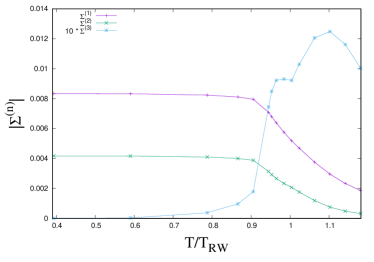
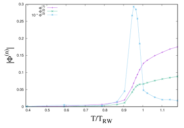
Figure 3: The $T$-dependence of dual quark with $n=1$, $2$ and $3$.

Interestingly, $\Sigma^{(3)}$ behaves as similar with the Polyakov loop unlike the ordinary dual quark condensate. Therefore, we can use $\Sigma^{(3)}$ as the order parameter or the indicator of the confinement-deconfinement transition under the restriction of the integral range. Also, $n=3$ component shows non-monotonic behavior under the restriction; when we approach the RW endpoint temperature, $\Phi^{(3)}$ quickly approaches to small value.

VII Summary

In this article, we have investigated the meaning of the $\mathbb{Z}_{N_{\mathrm{c}}}$ images appearing in QCD at finite temperature ($T$) and imaginary chemical potential ($\mu_{\mathrm{I}}$). Particularly, to answer how the $\mathbb{Z}_{N_{\mathrm{c}}}$ images affect the thermal system, we have considered the canonical ensemble by using the grand-canonical ensemble via the Fourier transformation. In actual discussions, we employ the different representation of the expectation value via the Fourier transformation which is mathematically equivalent with the canonical ensemble method at zero real chemical potential; see Eq. (26).

When we integrate out the grand-canonical partition function, ${\cal Z}_{\mathrm{GC}}(T,\mu_{\mathrm{I}})$, from $\theta=\mu_{\mathrm{I}}/T=-\pi$ to $\pi$ to construct the canonical partition function with fixed quark number ($Q$), only the $Q=0~{}\mathrm{mod}~{}3$ sector contributes to the thermodynamic system. However, the Polyakov-loop paradox appears in this case; the expectation value of the Polyakov loop by using the canonical ensemble becomes infinity or $0$ after removing the unphysical sectors and it is inconsistent with the value calculated from the grand-canonical ensemble. This paradox is coursed from the fact that the Polyakov loop does not have the Roberge-Weiss periodicity which is the special property of QCD grand-canonical partition function at finite $\theta:=\mu_{\mathrm{I}}/T$.

To discuss the Polyakov-loop paradox, we revisit the modified Polyakov-loop. Then, the expectation value of the Polyakov loop ($\Phi$) can be constructed from the modified Polyakov-loop ($\Psi=e^{i\theta}\Phi$) which is the RW periodic quantity. In the case of the RW periodic quantities, only the $Q=0~{}\mathrm{mod}~{}3$ sector contributes the thermodynamic system and then we can prove the relation, $\langle\Psi\rangle_{\mathrm{GC}}=\langle\Phi\rangle_{\mathrm{GC}}$, at least with zero real chemical potential. Thus, there is no Polyakov-loop paradox.

From the RW periodicity issue of the modified Polyakov-loop, we can restrict the integral range from $-\pi\sim\pi$ to $-\pi/3\sim\pi/3$ because of the property of the Fourier transformation. Actually, we can correctly reproduce the chiral condensate and also the Polyakov loop by using this restriction. This result strongly indicates that the non-trivial $\mathbb{Z}_{3}$ images are unphysical and we must remove it from the Fourier transformation when we construct the canonical ensemble. Following the restriction, we can well determine the dual quark condensate; in the ordinary determination, we must break the RW periodicity by hand, but now we do not need such unclear procedure. We have demonstrated the $T$-dependence of each canonical sector of the chiral condensate and the Polyakov loop by using the PNJL model under the restriction of the integral range.

Recently, it is proposed that the structure of QCD at finite $\mu_{\mathrm{I}}$ may be related with the confinement-deconfinement transition Kashiwa and Ohnishi (2015); *Kashiwa:2016vrl; *Kashiwa:2017yvy based on the analogy of the topological order at $T=0$ Wen (1990); Sato (2008) and thus it is interesting to know detailed properties of QCD at finite $\mu_{\mathrm{I}}$. We hope that this analysis shed a light to mysterious property of the confinement-deconfinement transition.