Scattering amplitudes from finite-volume spectral functions

Abstract

A novel proposal is outlined to determine scattering amplitudes from finite-volume spectral functions. The method requires extracting smeared spectral functions from finite-volume Euclidean correlation functions, with a particular complex smearing kernel of width $\epsilon$ which implements the standard $i\epsilon$-prescription. In the $L\rightarrow\infty$ limit these smeared spectral functions are therefore equivalent to Minkowskian correlators with a specific time ordering to which a modified LSZ reduction formalism can be applied. The approach is presented for general $m\rightarrow n$ scattering amplitudes (above arbitrary inelastic thresholds) for a single-species real scalar field, although generalization to arbitrary spins and multiple coupled channels is likely straightforward. Processes mediated by the single insertion of an external current are also considered. Numerical determination of the finite-volume smeared spectral function is discussed briefly and the interplay between the finite volume, Euclidean signature, and time-ordered $i\epsilon$-prescription is illustrated perturbatively in a toy example.

I Introduction

The determination of real-time scattering amplitudes from Euclidean lattice field theory simulations is challenging. It was pointed out long ago by Maiani and Testa Maiani:1990ca that on-shell scattering amplitudes away from threshold cannot be obtained from the asymptotic temporal separation of infinite-volume Euclidean correlation functions. Calculations of finite-volume energies and matrix elements in Monte Carlo simulations, however, employ $n$-point correlation functions in which all time separations are taken asymptotically large. The challenge of extracting on-shell scattering information is partly resolved by Lüscher’s method, in which finite-volume two-hadron energies are related to elastic scattering amplitudes Luscher:1990ux by a determinant equation. This relation is widely used in numerical simulations and has been extended to non-zero total momenta Rummukainen:1995vs ; Kim:2005gf ; Fu:2011xz , coupled two-hadron scattering channels He:2005ey ; Lage:2009zv ; Bernard:2010fp ; Briceno:2012yi ; Hansen:2012tf , asymmetric volumes Feng:2004ua , non-zero spin Gockeler:2012yj ; Briceno:2014oea ; Morningstar:2017spu , and amplitudes with external currents Lellouch:2000pv ; Lin:2001ek ; Meyer:2011um ; Briceno:2012yi ; Hansen:2012tf ; Briceno:2014uqa ; Briceno:2015csa ; Briceno:2015tza ; Baroni:2018iau . The extension of the method to treat three-particle amplitudes is currently under development Briceno:2012rv ; Polejaeva:2012ut ; Hansen:2014eka ; Meissner:2014dea ; Hansen:2015zga ; Briceno:2017tce ; Mai:2017bge ; Hammer:2017uqm ; Hammer:2017kms ; Doring:2018xxx ; Briceno:2018aml ; Romero-Lopez:2018rcb ; Hansen:2019nir ; Blanton:2019igq .

The main limitations of this finite-volume approach are as follows:

• It is limited to energies below three or more particle thresholds. Once the three-particle formalism is fully developed, it will be possible to treat all energies below four-particle thresholds. Such restrictions become increasingly severe for lattice QCD simulations as the light quark masses are lowered to their physical values and below. Application of the three-particle formalism also requires as input the two-to-two amplitude over a continuous range of energies, necessitating a parametrization and extrapolation.

• The determinant equations for two-to-two amplitudes are block diagonalized in finite-volume irreps of the relevant total-momentum little group, mixing infinite-volume partial waves. These relations are infinite dimensional, and are therefore truncated at some partial wave $\ell_{\max}$. The systematic error due to this truncation must be assessed, but is small near threshold due to the angular-momentum barrier. Conversely, higher partial wave amplitudes are sub-leading and thus difficult to determine. Furthermore, this necessary projection onto partial waves and finite-volume irreps prevents the direct calculation of inclusive processes via the optical theorem.

• The determination of individual finite-volume energies and matrix elements becomes cumbersome in large spatial volumes. On one ensemble with $m_{\pi}L=6.1$ from a recent lattice QCD calculation of elastic pion-pion scattering Andersen:2018mau , $43$ energies are determined, while another recent $\rho\pi$ scattering calculation Woss:2018irj (performed at heavy quark masses so the $\rho$ is stable) employs 141 energies across two volumes with $m_{\pi}L=10.3$ and $12.4$. The increasingly dense finite-volume spectrum and the simultaneously decreasing magnitude of the desired finite volume effects makes the large volume limit of this formalism intractable.

• The determinant condition for a single finite-volume energy involves amplitudes from all total spins and open scattering channels, so that particular initial and final states are selected only in special situations. A model parametrization is therefore required to simultaneously extract all relevant amplitudes when fitting the finite-volume energies.

Despite these restrictions, substantial progress has been made in lattice calculations of hadron scattering amplitudes. Calculations of the energy dependence of elastic scattering amplitudes between pseudoscalar mesons have provided valuable determinations of the quark-mass dependence of the low-lying resonances Andersen:2018mau ; Alexandrou:2017mpi ; Bulava:2016mks ; Fu:2016itp ; Guo:2016zos ; Briceno:2016mjc ; Wilson:2015dqa ; Feng:2014gba ; Dudek:2012xn ; Pelissier:2012pi ; Aoki:2011yj ; Lang:2011mn ; Feng:2010es . These results have sufficient statistical precision to begin addressing systematics due to the finite volume and lattice spacing. Meson-baryon and baryon-baryon calculations Andersen:2017una ; Lang:2016hnn ; Lang:2012db ; Detmold:2015qwf ; Berkowitz:2015eaa ; Orginos:2015aya are considerably less developed while pioneering calculations which treat multiple coupled two-particle channels Briceno:2017qmb ; Moir:2016srx ; Dudek:2016cru ; Wilson:2014cna ; Mohler:2013rwa have been performed. Calculations of transition amplitudes involving external currents are presented in Refs. Andersen:2018mau ; Alexandrou:2018jbt ; Briceno:2016kkp ; Feng:2014gba and scattering involving vector bosons is treated in Refs. Romero-Lopez:2018zyy ; Woss:2018irj .

However, the restrictions listed above have so far prevented the quantitative study of scattering amplitudes in many interesting systems. For example, potentially exotic hadrons with hidden heavy-flavor quantum numbers couple significantly to multiple two-hadron decay channels Olsen:2017bmm ; Guo:2017jvc ; Lebed:2016hpi ; Esposito:2016noz ; Chen:2016qju , all of which occur above many inelastic thresholds so that the currently-available finite-volume formalism is inapplicable. A similar problem exists for lattice QCD studies of excited baryon resonances in the $1-3{\rm GeV}$ region, for which polarization observables and higher partial waves are needed phenomenologically Proceedings:2018uig . Even low-lying hadronic resonances such as the $N(1440)$ (Roper), $\rho(770)$, $K^{*}(892)$, and $\Delta(1232)$ are located above $n\geq 3$ hadron thresholds. Although such effects formally must be treated, they are likely less important for resonances with a weak coupling to $n\geq 3$ hadron states.

The wealth of existing experimental data on hadron scattering, ongoing and future experiments, and the ever-increasing physical volume of lattice QCD simulations motivate exploration of alternatives to the finite-volume approach. A first step in this direction is Ref. Hansen:2017mnd which outlines a method to obtain single-hadron inclusive transition rates above arbitrary inelastic thresholds from Euclidean lattice simulations without employing the finite volume. Ref. Hansen:2017mnd advocates using spectral functions obtained in Euclidean time and finite volume, defined as

$$C_{\bm{p}_{1}\bm{p}_{1}}^{L,J}(\tau) =2E(\bm{p}_{1})L^{3}\langle\bm{p}_{1}|\hat{J}\,{\rm e}^{-\hat{H}\tau}\,\hat{J}^{\dagger}|\bm{p}_{1}\rangle_{L}=\int_{0}^{\infty}\frac{dE}{\pi}\,\rho_{\bm{p}_{1}\bm{p}_{1}}^{L,J}(E)\,\mathrm{e}^{-E\tau}\,,\qquad$$ (1)

$$\rho_{\bm{p}_{1}\bm{p}_{1}}^{L,{J}}(E) =2E(\bm{p}_{1})L^{3}\sum_{n}\pi\,\delta(E-E^{L}_{n})\,|\langle\bm{p}_{1}|\hat{J}|n\rangle_{L}|^{2}\,,$$ (2)

where $E(\bm{p}_{2})\equiv\sqrt{\bm{p}_{2}^{2}+m^{2}}$ and $m$ the physical mass. Here the ‘endcap’ state $|\bm{p}_{1}\rangle_{L}$ is a finite-volume one-particle state (with other internal indices suppressed), $\hat{J}$ a local external current mediating the transition (possibly projected onto definite three-momentum), and $\hat{H}$ the Hamiltonian. The sum over $n$ runs over all finite-volume Hamiltonian eigenstates, with corresponding energies given by $\{E_{n}^{L}\}$.

At first glance $\rho_{\bm{p}_{1}\bm{p}_{1}}^{L,J}(E)$, a sum over $\delta$-functions, is qualitatively different from its continuous infinite-volume counterpart. Ref. Hansen:2017mnd suggests bridging this gap via the Backus-Gilbert approach to inverse problems BG1 ; BG2 which yields a smeared spectral function

$$\hat{\rho}_{\bm{p}_{1}\bm{p}_{1}}^{L,J,\epsilon}(E)=\int_{0}^{\infty}\frac{d\omega}{\pi}\,\hat{\delta}_{\epsilon}(E,\omega)\,\rho_{\bm{p}_{1}\bm{p}_{1}}^{L,J}(\omega)\,,\qquad\int_{0}^{\infty}\frac{d\omega}{\pi}\,\hat{\delta}_{\epsilon}(E,\omega)=1\,.$$ (3)

Eq. 3 introduces the smearing kernel $\lim_{\epsilon\rightarrow 0^{+}}\hat{\delta}_{\epsilon}(E,\omega)=\pi\delta(E-\omega)$ with a characteristic width $\epsilon$ that compromises between resolution and numerical stability. The infinite-volume spectral function, from which the total transition rate is easily obtained, is recovered from the ordered double limit $\rho_{\bm{p}_{1}\bm{p}_{1}}^{J}(E)=\lim_{\epsilon\rightarrow 0^{+}}\,\lim_{L\rightarrow\infty}\hat{\rho}_{\bm{p}_{1}\bm{p}_{1}}^{L,J,\epsilon}(E)$. This procedure nicely circumvents the Maiani-Testa no-go theorem Maiani:1990ca by not taking the asymptotic time limit $t\rightarrow\infty$ typical in calculations of finite-volume energies and matrix elements. Although Ref. Hansen:2017mnd provides tests in a toy model, an application to zero-temperature lattice data has not yet been published.

This work describes a generalization of Ref. Hansen:2017mnd in which the Lehmann-Symanzik-Zimmermann (LSZ) reduction formalism is used to determine arbitrary scattering amplitudes from finite-volume spectral functions. Processes mediated by a single local external current are also included in addition to purely hadronic processes without such currents. As a first example, consider the spectral function from Eq. 1 with pion endcaps and $\hat{J}$ set to the temporal component of the axial current at definite momentum $\bm{p}_{2}$. The formalism of Ref. Hansen:2017mnd yields the inclusive rate for the process $\pi(\bm{p}_{1})+A_{0}(\bm{p}_{2})\rightarrow X$ at an arbitrary four-momentum transfer determined by the energy argument $E$.

Since $\hat{A}_{0}(\bm{p}_{2})$ has the quantum numbers of a single pion of momentum $\bm{p}_{2}$, the rate for $\pi(\bm{p}_{1})+A_{0}(\bm{p}_{2})\rightarrow X$ develops a pole when the energy carried by the current coincides with the on-shell value $E=E(\bm{p}_{2})$. The residue at this pole then gives the purely hadronic inclusive rate $\pi(\bm{p}_{1})+\pi(\bm{p}_{2})\rightarrow X$. Taking this approach further, Sec. IV.2 demonstrates that a different choice of smearing kernel can be employed in Eq. 3 (to the same underlying spectral function) to implement the $i\epsilon$-prescription in the analytic continuation to real scattering energies, thereby defining a quantity that coincides with the exclusive scattering amplitude, rather than the inclusive rate, in the ordered double limit.

In contrast to the total rates considered in Ref. Hansen:2017mnd , scattering amplitudes are complex-valued functions with the real and imaginary parts related by unitarity constraints. However, the correlator $C_{\bm{p}_{1}\bm{p}_{1}}^{L,J}(\tau)$ is pure real so that the complexity enters only through the specific definition of the smearing kernel, which takes the form of a complex-valued pole. An important result of this work is that the practitioner can choose the value of $i\epsilon$ in the pole, and that this parameter is distributed through all unitarity cuts to ensure a well-defined $L\to\infty$ limit. In direct analogy to Ref. Hansen:2017mnd , one requires a hierarchy of scales $1/L\ll\epsilon\ll m$ to access the desired amplitudes. However, the perturbative example of Sec. V indicates that known aspects of the $\epsilon$-dependence may lead to a milder extraction problem than in the case of total rates.

A final important distinction compared to Ref. Hansen:2017mnd is that in contrast to a renormalized current, a single-particle interpolation field is not uniquely defined. This is treated in the present approach exactly as in the LSZ formalism, by approaching the pole and dividing out the operator overlap factor. The freedom to choose an interpolating operator may thus be used to give better constraints on the extraction of the amplitude. To this end it is important to note that in the example above the second pion interpolator should not be optimized to maximally overlap a single finite-volume state. In contrast, overlapping multiple states is crucial as it is the sum over these that leads to the estimated scattering amplitude.

Preceding Ref. Hansen:2017mnd , prospects for extracting the hadronic tensor by solving the inverse problem on a Euclidean four-point function are discussed and tested in Refs. Liu:1993cv ; Liu:2016djw ; Liu:2017lpe . In contrast to Ref. Hansen:2017mnd and this article, these earlier publications do not explore the role of smearing nor of finite-volume effects. Another interesting direction is discussed in Ref. Hashimoto:2017wqo , which details an exploratory lattice study of Euclidean four-point functions relevant for semi-leptonic $B$-decays. Ref. Hashimoto:2017wqo advocates avoiding the inverse problem by integrating experimental data against a multi-pole function to extract moments that can be directly compared to lattice data.

It is also worth considering the relation of the present work to Ref. Agadjanov:2016mao , which describes a method for extracting the optical potential from a lattice calculation. The approach of Ref. Agadjanov:2016mao requires reconstructing the finite-volume optical potential, known to contain an infinite tower of poles, by fitting a function of this form, applying an $i\epsilon$-prescription, and finally estimating the limit $L\to\infty$ followed by $\epsilon\to 0$. The ordered double limit is a common feature but this earlier work differs in that it is based on measuring finite-volume energies (with twisted boundary conditions) and inserting the $i\epsilon$ via a fit function.

Finally, Ref. Barata:1990rn considers the extent to which scattering amplitudes can be reconstructed from Euclidean field theories, but from a formal perspective. That work is motivated by conceptual problems that originate in the nonuniqueness of discretization effects together with the role of the continuum limit in defining the analytic continuation to Minkowski signature. These issues are avoided here by expressing the relation through the finite-volume spectral function.

As explained in Sec. II, an arbitrary $m$-to-$n$ particle amplitude requires a (complex) spectral function with $r=m+n-2$ energy arguments, with one fewer argument if no external current is included and one more if either $m$ or $n$ is zero. Proposals for efficiently isolating the scattering amplitude within the spectral function are discussed in Sec. III although no numerical results are presented. For simplicity of notation, the method is illustrated for a single component real scalar field.

A number of different approaches can be used to determine $\hat{\rho}_{\bm{p}_{1}\bm{p}_{1}}^{L,J,\epsilon}(E)$ from $C_{\bm{p}_{1}\bm{p}_{1}}^{L,J}(\tau)$ and this work is agnostic to the method employed. It is however crucial that the resolution function, $\hat{\delta}_{\epsilon}(\omega,E)$, approximates the specific complex pole form. Sec. III includes a brief discussion of the various possibilities, including the use of a variational method to explicitly build up the spectral function by individually extracting the finite-volume energies and matrix elements. Some probable first applications of the general formalism are presented in Sec. IV. Sec. V details a perturbative test elucidating the interplay between real and imaginary time, the finite volume, the smearing kernel, and the $i\epsilon$-prescription. The outlook and conclusions are in Sec. VI together with some brief remarks on the straightforward generalization to multiple species of complex arbitrary spin fields.

II LSZ reduction

This section details the somewhat non-standard application of the LSZ reduction approach used in this work and is therefore restricted to infinite-volume Minkowski correlators. The main result given in Eq. 12 is the relation between a smeared spectral function with a particular smearing kernel and the exclusive $m$-to-$n$ scattering amplitude for the process $\bm{p}_{1}+\cdots+\bm{p}_{m}+J\rightarrow\bm{p}_{m+1}+\cdots+\bm{p}_{m+n}$ which is mediated by the external local current $\hat{J}(x)$. It is assumed that $m$ and $n$ are non-zero for clarity of this general presentation. Zero-to-two transitions are discussed in Sec. IV.1. The expressions for a purely hadronic process with no external current are provided at the end of the section, culminating in the analogous main result in Eq. 16.

For simplicity of notation consider an arbitrary theory with a single real scalar field. The LSZ formalism LSZ holds under several assumptions including the existence of a mass gap, complicating the application to lattice QCD+QED unless the photon is given a non-zero mass. Based on the asymptotic conditions of Haag-Ruelle scattering theory Haag ; Ruelle , there is some generality in the $n$-point functions to which the LSZ reduction is applied. The LSZ procedure is conventionally applied to connected time-ordered Feynman functions

$$\widetilde{G}_{\rm c}^{J}(q_{1},\dots,q_{m+n})=\int\prod_{j=1}^{m+n}\left\{d^{4}x_{j}\,{\rm e}^{-iq_{j}\cdot x_{j}}\right\}\langle 0|T\left\{\hat{\phi}(x_{1})\cdots\hat{\phi}(x_{m+n})\hat{J}(0)\right\}|0\rangle_{\rm c}\,,$$ (4)

where $q_{j}\cdot x_{j}=q_{j}^{0}t_{j}-\bm{q}_{j}\cdot\bm{x}_{j}$, $\hat{\phi}(x)$ is a suitable interpolating operator for a single-component real scalar field, and $\bm{q}_{j}=\pm\bm{p}_{j}$. The integrals defining the Fourier transform are well-defined (once an ultraviolet regularization is put in place) because of the implicit $i\epsilon$-prescription in the Hamiltonian, $\hat{H}\to\hat{H}-i\epsilon$. This same prescription can be encoded in the momentum coordinates via the replacement $q_{j}^{0}\rightarrow q_{j}^{0}\pm i\epsilon$, which is applied in all temporal Fourier transforms. The fully-connected amplitude ${\cal M}_{\rm c}^{J}(p_{m+n}\cdots p_{m+1}|p_{m}\cdots p_{1})$ (where the $\{p_{j}\}$ are on-shell four momenta) is then obtained from the residue of the pole in $\widetilde{G}_{\rm c}^{J}(q_{1},\dots,q_{m+n})$ as $q_{j}^{0}\rightarrow\pm E(\bm{p}_{j})$. The upper (lower) signs for both the energy-momentum coordinates and the $i\epsilon$ are taken for incoming (outgoing) particles, respectively.

Rather than using spectral functions from the time-momentum representation of the $(m+n+1)$-point Feynman functions in Eq. 4, we instead define alternative $(m+n-1)$-point functions in which the integration runs over a single time ordering. The latter are referred to as ‘endcap functions’

$$\widetilde{F}_{\bm{p}_{m+n}\bm{p}_{1}}^{J}(q_{r+1},\dots,q_{2})=\int\prod_{j=2}^{r+1}\left\{d^{4}x_{j}\,{\rm e}^{-iq_{j}\cdot x_{j}}\right\}\,\theta(t_{r+1}-t_{r})\cdots\theta(t_{m+1})\,\\[-5.0pt] \times\theta(-t_{m})\cdots\theta(t_{3}-t_{2})\,\langle\bm{p}_{m+n}|\hat{\phi}(x_{r+1})\cdots\hat{\phi}(x_{m+1})\,\hat{J}(0)\hat{\phi}(x_{m})\cdots\hat{\phi}(x_{2})|\bm{p}_{1}\rangle_{\rm c}\,,$$ (5)

where $|\bm{p}\rangle$ denotes a one-particle state with the usual normalization $\langle\bm{p}^{\prime}|\bm{p}\rangle=2E(\bm{p})(2\pi)^{3}\delta^{3}(\bm{p}^{\prime}-\bm{p})$, and $r=(m+n-2)$ Heaviside step functions are used to enforce a particular time ordering. Note that it would make no difference to include a time ordering operator in the matrix element in this expression. Spectral functions introduced from the time-momentum representations of endcap functions have $r$ arguments, rather than the $r+2$ required for Feynman functions, and thus are presumably more amenable to numerical determination. Furthermore, the selection of a single time ordering requires only a single spectral function whereas one is required for each of the time orderings in Eq. 4. The full Lorentz covariance of the Feynman functions is lost when the endcaps and a single time ordering are employed, but is of course recovered in the scattering amplitude.

Although the analytic structure of the endcap functions in Eq. 5 is different than that of the Feynman functions of Eq. 4, it is demonstrated in App. A that LSZ reduction of $r$ interpolating fields yields the same on-shell pole

$$\widetilde{F}_{\bm{p}_{m+n}\bm{p}_{1}}^{J}(q_{m+n-1},\dots,q_{2})=\prod_{j=2}^{r+1}\left\{\frac{Z^{1/2}(\bm{p}_{j})}{2E(\bm{p}_{j})}\right\}\,{\cal M}_{\rm c}^{J}(p_{m+n}\cdots p_{m+1}|p_{m}\cdots p_{1})\,\\ \times\prod_{j=2}^{m}\left\{\frac{i}{q_{j}^{0}-E(\bm{p}_{j})+i\epsilon}\right\}\prod_{k=m+1}^{r+1}\left\{\frac{i}{-q_{k}^{0}-E(\bm{p}_{k})+i\epsilon}\right\}\,+\cdots\,,$$ (6)

where $Z^{1/2}(\bm{p})=\langle\bm{p}|\hat{\phi}(0)|0\rangle$ and ‘$+\cdots$’ denotes additional contributions which are regular near the pole. The endcap function in Eqs. 5 and 6 can also be expressed as a spectral function

$$\widetilde{F}_{\bm{p}_{m+n}\bm{p}_{1}}^{J}(q_{r+1},\dots,q_{2})=\hat{\rho}_{\bm{p}_{m+n}\bm{p}_{1}}^{J,\epsilon}(q_{r+1},\dots,q_{2})\equiv\int_{0}^{\infty}\!\!\frac{d^{r}\!E}{\pi^{r}}\ \hat{\delta}^{r}_{\epsilon}(q^{0},E)\,\rho_{\bm{p}_{m+n}\bm{p}_{1}}^{J}\!\big{(}(E_{r+1},-\bm{p}_{r+1}),\dots,(E_{2},\bm{p}_{2})\big{)}\,,$$ (7)

where

$$\int_{0}^{\infty}\!\!\frac{d^{r}\!E}{\pi^{r}} \equiv\prod_{j=2}^{r+1}\left\{\int_{0}^{\infty}\frac{dE_{j}}{\pi}\right\}\,,$$ (8)

$$\hat{\delta}^{r}_{\epsilon}(q^{0},E) \equiv\prod_{k=m+1}^{r+1}\left\{\frac{i}{E(\bm{p}_{m+n})-\sum_{l=k}^{r+1}q_{l}^{0}-E_{k}+i\epsilon}\right\}\times\prod_{k=2}^{m}\left\{\frac{i}{\sum_{l=2}^{k}q_{l}^{0}+E(\bm{p}_{1})-E_{k}+i\epsilon}\right\}\,,$$ (9)

$$\begin{split}\rho_{\bm{p}_{m+n}\bm{p}_{1}}^{J}(k_{r+1},\dots,k_{2})&\equiv\sum_{\alpha_{r+1},\dots,\alpha_{2}}\prod_{j=2}^{r+1}\left\{\pi\delta(E_{\alpha_{j}}-k_{j}^{0})\right\}\times\langle\bm{p}_{m+n}|\hat{\varphi}(\bm{k}_{r+1},0)|\alpha_{r+1}\rangle\times\cdots\times\\[-5.0pt] &\hskip 150.0pt\times\langle\alpha_{m+1}|\hat{J}(0)|\alpha_{m}\rangle\times\cdots\times\langle\alpha_{2}|\hat{\varphi}(\bm{k}_{2},0)|\bm{p}_{1}\rangle\,-\cdots\,.\end{split}$$ (10)

Here $\hat{\varphi}(\bm{p},t)=\int d^{3}\bm{x}\,{\rm e}^{i\bm{p}\cdot\bm{x}}\hat{\phi}(\bm{x},t)$, $E_{\alpha}$ is the energy of the state $|\alpha\rangle$, and the ellipsis denotes disconnected contributions which must be subtracted explicitly. The sums of states indexed by $\alpha_{j}$ are shorthand for individual integrals over each of the fixed-particle-number sectors of the Hilbert space of states, formally defined as Hansen:2017mnd

$$\sum_{\alpha}\equiv\sum_{n_{\alpha}}\frac{1}{n_{\alpha}!}\int\prod_{j=1}^{n_{\alpha}}d\Gamma(\bm{k}_{j})\,,$$ (11)

where $d\Gamma(\bm{k})\equiv\frac{d^{3}\bm{k}}{(2\pi)^{3}\,2E(\bm{k})}$ is the usual Lorentz-invariant integration measure. Because these relations are employed at finite $\epsilon$, the particular form of the pole factors introduced above must be maintained throughout and not manipulated using infinitesimal-$\epsilon$ identities.

As already suggested by the notation, the central idea of our proposal is to view the pole factors in Eq. 9 as complex smearing functions akin to $\hat{\delta}_{\epsilon}(E,\omega)$ in Eq. 3. Eq. 7 thus defines the smeared spectral function $\hat{\rho}_{\bm{p}_{m+n}\bm{p}_{1}}^{J,\epsilon}(q_{r+1},\dots,q_{2})$ with characteristic width $\epsilon$. Based on Eq. 6, the desired amplitude is obtained from the limit

$${\cal M}_{\rm c}^{J}(p_{m+n}\cdots p_{m+1}|p_{m}\cdots p_{1})=\prod_{j=2}^{r+1}\frac{2E(\bm{p}_{j})}{Z^{1/2}(\bm{p}_{j})}\,\times\lim_{\epsilon\rightarrow 0^{+}}\,\epsilon^{r}\hat{\rho}_{\bm{p}_{m+n}\bm{p}_{1}}^{J,\epsilon}\big{(}(-E(\bm{p}_{r+1}),-\bm{p}_{r+1}),\dots,(E(\bm{p}_{2}),\bm{p}_{2})\big{)}\,,$$ (12)

where the arguments of the smeared spectral function have been set on shell and the poles in Eq. 6 amputated by the factor $\epsilon^{r}$. Practically, the smeared spectral function at finite $\epsilon$, $\hat{\rho}_{\bm{p}_{m+n}\bm{p}_{1}}^{J,\epsilon}(q_{r+1},\dots,q_{2})$, is obtained from the $L\rightarrow\infty$ limit of finite-volume spectral functions with a particular smearing kernel. The relation in Eq. 12 between amplitudes and smeared spectral functions in the $\epsilon\rightarrow 0^{+}$ limit is a central tenet of the method. The overlap factors $Z(\bm{p})$ are in fact independent of $\bm{p}$ due to Lorentz covariance but their momentum dependence is retained as a notational reminder that arbitrary interpolators may be used for each of the particles. These overlap factors do acquire momentum dependence if calculated in a finite volume or if a spatial smearing wavefunction is introduced.

For completeness, we close by giving the formulae for endcap functions $\widetilde{F}_{\bm{p}_{m+n}\bm{p}_{1}}(q_{r+1},\dots,q_{2})$ that do not contain an external current. The LSZ reduction in Eq. 6 now contains an overall four-momentum conserving $\delta$-function which we omit from the definition of the spectral function

$$\widetilde{F}_{\bm{p}_{m+n}\bm{p}_{1}}(q_{r+1},\dots,q_{2})=(2\pi)^{4}\delta^{4}(p_{m+n}-q_{r+1}-\cdots-q_{2}-p_{1})\,\hat{\rho}^{\epsilon}_{\bm{p}_{m+n}\bm{p}_{1}}(q_{r+1},\dots,q_{m+2},q_{m},\dots,q_{2})\,,$$ (13)

where the smeared spectral function has now has $r-1$ energy-momentum arguments chosen to omit $q_{m+1}$. The smeared and unsmeared spectral functions are given by

$$\begin{split}\hat{\rho}^{\epsilon}_{\bm{p}_{m+n}\bm{p}_{1}}(q_{r+1},\dots,q_{m+2},q_{m},\dots,q_{2})&=\int_{0}^{\infty}\,\frac{d^{r-1}E}{\pi^{r-1}}\hat{\delta}^{r-1}_{\epsilon}(q^{0},E)\\ &\times\rho_{\bm{p}_{m+n}\bm{p}_{1}}\big{(}(E_{r+1},-\bm{p}_{r+1}),\dots,(E_{m+2},\bm{p}_{m+2}),(E_{m},\bm{p}_{m}),\dots,(E_{2},\bm{p}_{2})\big{)}\,,\end{split}$$ (14)

$$\begin{split}\rho_{\bm{p}_{m+n}\bm{p}_{1}}(k_{r+1},\dots,k_{m+2},k_{m+1},\dots,k_{2})&\equiv\sum_{\alpha_{r+1},\dots,\alpha_{m+2},\atop\alpha_{m},\dots,\alpha_{2}}\prod_{j=2,\atop j\neq m+1}^{r+1}\left\{\pi\delta(E_{\alpha_{j}}-k_{j}^{0})\right\}\times\langle\bm{p}_{m+n}|\hat{\varphi}(\bm{k}_{r+1},0)|\alpha_{r+1}\rangle\\[0.0pt] &\hskip 70.0pt\times\cdots\times\langle\alpha_{m+2}|\hat{\phi}(0)|\alpha_{m}\rangle\times\cdots\times\langle\alpha_{2}|\hat{\varphi}(\bm{k}_{2},0)|\bm{p}_{1}\rangle\,-\cdots\,,\end{split}$$ (15)

where the disconnected contributions are again subtracted and the integration measure $\frac{d^{r-1}E}{\pi^{r-1}}$ omits $E_{m+1}$. Similarly, the smearing kernel $\hat{\delta}^{r-1}_{\epsilon}(q^{0},E)$ is defined as in Eq. 9 but with $\prod_{k=m+2}^{r+1}$ in the first factor.

The amplitude is recovered as in Eq. 12

$$i{\cal M}_{\rm c}(p_{m+n}\cdots p_{m+1}|p_{m}\cdots p_{1})=\prod_{j=2}^{r+1}\frac{2E(\bm{p}_{j})}{Z^{1/2}(\bm{p}_{j})}\,\\ \times\lim_{\epsilon\rightarrow 0^{+}}\,\epsilon^{r}\hat{\rho}_{\bm{p}_{m+n}\bm{p}_{1}}^{\epsilon}\big{(}(-E(\bm{p}_{r+1}),-\bm{p}_{r+1}),\dots,(-E(\bm{p}_{m+2}),-\bm{p}_{m+2}),(E(\bm{p}_{m}),\bm{p}_{m}),\dots,(E(\bm{p}_{2}),\bm{p}_{2})\big{)}\,,$$ (16)

with the conventional factor of $i$ included in its definition. Note that although $r-1$ pole factors have been introduced in the smearing kernel, the LSZ reduction necessitates that $r$ such poles must be amputated at the on-shell point. This subtlety is discussed further in Sec. V.

III Calculation of the spectral functions

The smeared spectral function defined in Eq. 7 can be obtained from finite-volume Euclidean lattice simulations. To this end, we employ connected $(m+n+1)$-point and two-point Euclidean correlation functions in the time-momentum representation

$$C^{J,L}_{(m+n+1){\rm pt}}\big{(}(-\bm{p}_{n+m},\tau_{n+m}),\dots,(\bm{p}_{1},\tau_{1})\big{)} ={\langle}0|\hat{\varphi}(-\bm{p}_{n+m},\tau_{n+m})\dots\hat{J}(0)\dots\hat{\varphi}(\bm{p}_{1},\tau_{1})|0\rangle_{{\rm c},L}\,,$$ (17)

$$C^{L}_{2{\rm pt}}(\bm{p},\tau) ={\langle}0|\hat{\varphi}(\bm{p},\tau)\hat{\phi}(0)|0\rangle_{{\rm c},L}\,,$$ (18)

where $\tau_{n+m}>\tau_{n+m-1}>\cdots>\tau_{m+1}>0>\tau_{n}>\cdots>\tau_{1}$, and $\hat{\varphi}(\bm{p},\tau)=\int_{\Omega_{L}}d^{3}\bm{x}\,{\rm e}^{i\bm{p}\cdot\bm{x}}\hat{\phi}(x)$ where $\Omega_{L}$ denotes the periodic three-torus of size $L$. Note that only finite-volume momenta $\bm{p}=2\pi\bm{n}/L$, where $\bm{n}$ is a vector of integers, are possible. These correlation functions are amenable to calculation with lattice simulations, and are used to define Euclidean endcap functions

$$\begin{split}C^{J,L}_{\bm{p}_{n+m}\bm{p}_{1}}\big{(}(-\bm{p}_{r+1},\tau_{r+1}),\dots,(\bm{p}_{2},\tau_{2})\big{)}&=2\sqrt{E(\bm{p}_{n+m})E(\bm{p}_{1})}L^{3}Z^{1/2}(\bm{p}_{n+m})Z^{1/2}(\bm{p}_{1})\,\\ &\hskip 50.0pt\times\lim_{{\tau_{n+m}-\tau_{r+1},\atop{\tau_{2}-\tau_{1}}}\rightarrow\infty}\frac{C^{J,L}_{(m+n+1){\rm pt}}\big{(}(-\bm{p}_{n+m},\tau_{n+m}),\dots,(\bm{p}_{1},\tau_{1})\big{)}}{C^{L}_{2{\rm pt}}(\bm{p}_{m+n},\tau_{m+n}-\tau_{r+1})\,C^{L}_{2{\rm pt}}(\bm{p}_{1},\tau_{2}-\tau_{1})}\,,\end{split}$$ (19)

$$=2\sqrt{E(\bm{p}_{n+m})E(\bm{p}_{1})}L^{3}{\langle}\bm{p}_{m+n}|\hat{\varphi}(-\bm{p}_{r+1},0)\,{\rm e}^{-\hat{H}(\tau_{r+1}-\tau_{r})}\cdots\hat{J}(0)\cdots{\rm e}^{-\hat{H}(\tau_{3}-\tau_{2})}\hat{\varphi}(\bm{p}_{2},0)|\bm{p}_{1}\rangle_{{\rm c},L}\,,$$ (20)

$$=\int_{0}^{\infty}\!\!\frac{d^{r}\!E}{\pi^{r}}{\rm e}^{-E_{r+1}(\tau_{r+1}-\tau_{r})}\cdots{\rm e}^{-E_{2}(\tau_{3}-\tau_{2})}\,\rho^{L,J}_{\bm{p}_{m+n}\bm{p}_{1}}\big{(}(E_{r+1},-\bm{p}_{r+1}),\dots,(E_{2},\bm{p}_{2})\big{)}\,,$$ (21)

where $\hat{H}$ is the finite-volume Hamiltonian and the two outermost fields have been placed on-shell by taking the asymptotic time separation limit. Throughout this work all finite-volume states are normalized to unity. A key observation is that the endcap function in Eq. 5 has a spectral function identical to the one in Eq. 21 in a suitably-defined $L\rightarrow\infty$ limit. Analytic continuation between the Minkowksi and Euclidean endcap functions thus proceeds via the spectral function, which is agnostic toward the metric signature.

The $L\to\infty$ limit is made well-defined by convolution with a resolution function, the specific choice of which determines the extracted quantity. In particular, using the $\hat{\delta}_{\epsilon}^{r}$ defined in the previous section we find

$$\hat{\rho}^{J,\epsilon}_{\bm{p}_{m+n},\bm{p}_{1}}(q_{r+1},\dots,q_{2})=\lim_{L\rightarrow\infty}\hat{\rho}^{L,J,\epsilon}_{\bm{p}_{m+n},\bm{p}_{1}}(q_{r+1},\dots,q_{2}),$$ (22)

where

$$\hat{\rho}_{\bm{p}_{m+n}\bm{p}_{1}}^{L,J,\epsilon}(q_{r+1},\dots,q_{2}) \equiv\int_{0}^{\infty}\!\!\frac{d^{r}\!E}{\pi^{r}}\ \hat{\delta}^{r}_{\epsilon}(q^{0},E)\,\rho_{\bm{p}_{m+n}\bm{p}_{1}}^{L,J}\!\big{(}(E_{r+1},-\bm{p}_{r+1}),\dots,(E_{2},\bm{p}_{2})\big{)}\,,$$ (23)

$$\begin{split}\rho_{\bm{p}_{m+n}\bm{p}_{1}}^{L,J}(k_{r+1},\dots,k_{2})&\equiv 2\sqrt{E(\bm{p}_{m+n})E(\bm{p}_{1})}L^{3}\sum_{n_{r+1},\dots,n_{2}}\prod_{j=2}^{r+1}\left\{\pi\delta(E^{L}_{n_{j}}-k_{j}^{0})\right\}\times\langle\bm{p}_{m+n}|\hat{\varphi}(\bm{k}_{r+1},0)|n_{r+1}\rangle_{L}\times\\ &\hskip 100.0pt\times\cdots\langle n_{m+1}|\hat{J}(0)|n_{m}\rangle_{L}\times\cdots\times\langle n_{2}|\hat{\varphi}(\bm{k}_{2},0)|\bm{p}_{1}\rangle_{L}\,-\cdots\,\end{split}$$ (24)

and the disconnected contributions to $\rho^{L,J}_{\bm{p}_{m+n}\bm{p}_{1}}$ are subtracted explicitly. As $L$ increases, the allowed finite-volume three-momenta will change. However, this difference becomes irrelevant as $L\rightarrow\infty$ due to the increasing density of states. The infinite-volume limit in Eq. 22 formally assumes that nearly equivalent finite-volume momenta are selected at each $L$.

So far we have not discussed algorithms for solving the inverse problem and determining the smeared spectral function $\hat{\rho}^{L,J,\epsilon}_{\bm{p}_{m+n},\bm{p}_{1}}$ from the Euclidean endcap functions $C^{J,L}_{\bm{p}_{n+m}\bm{p}_{1}}$. Much work in this direction has already been performed in both zero- and non-zero temperature lattice QCD, but typically with the aim of achieving a sharply peaked resolution function. Applications of the approach described here will require extensive numerical tests which are deferred to future work. Here we only comment briefly on some possible strategies.

First, the Backus-Gilbert method, discussed in Refs. BG1 ; BG2 , gives a linear, model-independent estimator of a smeared spectral function in which the covariance matrix of the data is used to stabilize the inverse. The algorithm was examined in the context of total hadronic rates in Ref. Hansen:2017mnd where the aim is to achieve a narrow resolution function with unit area, as indicated in Eq. 3. Ref. Hansen:2017mnd stresses that a perfect inverse, in which the resolution function becomes arbitrarily close to a $\delta$-function, is undesirable as it would lead to an extraction dominated by finite-$L$ effects. Instead, for a given box size, an optimal width exists that is larger than $1/L$ but, in the ideal situation, smaller than the scales over which the spectral function varies. In the present case, the desired resolution function is instead a complex pole form that is ultimately incorporated into the LSZ procedure.

In fact, as has been recently stressed in Ref. Hansen:2019idp , the Backus-Gilbert algorithm can be modified such that a target resolution function is viewed as an additional input. In this approach, the inverse is chosen to minimize the distance to the target function, rather than to minimize the width. This perspective is highly compatible with the method advocated here, allowing one to directly target the function $\hat{\rho}^{L,J,\epsilon}_{\bm{p}_{m+n},\bm{p}_{1}}$ with a specified value of $\epsilon$. Of course, any linear inverse method must face inherent limitations for a given input data quality. With this in mind we highlight two key features that might make the inverse problems considered here somewhat easier to treat.

• In contrast to the total rates in Ref. Hansen:2017mnd , the present method allows one to use a large basis of operators in the definition of the spectral function. These will all differ at finite $\epsilon$ but must coincide in the ordered double limit. Performing a constrained extrapolation to a set of spectral functions may better determine the target observable.

• The complex pole smearing function introduces an $\epsilon$-dependence with useful analyticity properties. In particular, amplitudes must have a convergent expansion in this parameter, with radius of convergence limited by the nearest branch point. This is in contrast to gaussian smearing kernels $\hat{\delta}_{\epsilon}(E,\omega)\sim\exp{[-(E-\omega)^{2}/\epsilon^{2}]}$, which exhibit an essential singularity at $\epsilon=0$. To this end note that for total-rate applications, the imaginary part of the complex pole ($\sim\epsilon/[(E-\omega)^{2}+\epsilon^{2}]$) may provide a more useful finite-width $\delta$-function approximation.

These features should allow one to maximally constrain the scattering amplitude without demanding too much resolution in the inverse.

In addition to Backus-Gilbert there are a number of other approaches to this well-known ‘unfolding’ problem due to its ubiquity. For example, the Maximum-Entropy Method (MEM) defines a likelihood function to determine the most probable solution for the available data set. To do so one requires a starting ansatz, referred to as the default model or prior estimate. In any finite-volume application, MEM clearly performs some smearing as the true finite-volume spectral function is a series of Dirac $\delta$-functions. However, in contrast to the Backus-Gilbert approach, the form of the resolution function is less clear.

Finally we emphasize that all finite-volume spectral functions are defined from finite-volume energies and matrix elements. These can, in principle, be accessed individually by employing solutions of Generalized Eigenvalue Problems (GEVP) using a large basis of interpolating operators Michael:1985ne ; Luscher:1990ck ; Blossier:2009kd . In this approach it is important to distinguish between the interpolating fields used to create the individual scattering particles, and the optimized operators used to access the finite-volume states. The latter do not enter the spectral function as they are divided out in determining finite-volume matrix elements, while the former appear as ‘current insertions’ which are put on the single-particle mass shell by selecting the appropriate four-momentum transfer. This exact finite-volume reconstruction is performed by using Eq. 24 in Eq. 23 to obtain

$$\hat{\rho}_{\bm{p}_{m+n}\bm{p}_{1}}^{L,J,\epsilon}(q_{r+1},\dots,q_{2})=2\sqrt{E(\bm{p}_{m+n})E(\bm{p}_{1})}L^{3}\sum_{n_{r+1},\dots,n_{2}}\hat{\delta}_{\epsilon}^{r}(q^{0},E^{L}_{n})\,\langle\bm{p}_{m+n}|\hat{\varphi}(\bm{k}_{r+1},0)|n_{r+1}\rangle_{L}\,\times\\ \times\cdots\times\langle n_{m+1}|\hat{J}(0)|n_{m}\rangle_{L}\times\cdots\times\langle n_{2}|\hat{\varphi}(\bm{k}_{2},0)|\bm{p}_{1}\rangle_{L}\,-\cdots\,,$$ (25)

where the disconnected contributions are subtracted and $\hat{\delta}_{\epsilon}^{r}(q^{0},E^{L}_{n})$ is short-hand for the smearing kernel of Eq. 9 with arguments $\{q^{0}_{r+1},\dots,q_{2}^{0}\}$ and $\{E^{L}_{n_{r+1}},\dots,E^{L}_{n_{2}}\}$. Practical applications of this finite volume reconstruction treat a few terms in the sum over $\{n_{r+1},\dots,n_{2}\}$ and are considered in Sec. IV. Such applications require the finite-volume energies and matrix elements shown in Eq. 24. Since the smearing kernel is peaked for small $\epsilon$, it is likely that only finite-volume states with energies $\{E^{L}_{n_{j}}\}$ near the on-shell point are important.

In addition to various reconstruction methods one can take advantage of known properties of the spectral function to potentially ameliorate the solution of this inverse problem. For example, it is likely that solving real inverse problems is preferable to the complex one in Eq. 22. To this end, the real and imaginary parts of $\hat{\rho}^{J,\epsilon}_{\bm{p}_{m+n},\bm{p}_{1}}(q_{r+1},\dots,q_{2})$ can be determined separately from solutions of four inverse problems. To see this note that the real and imaginary parts of $\hat{\rho}_{\bm{p}_{m+n}\bm{p}_{1}}^{L,J,\epsilon}$ can be trivially divided as follows

$$\text{Re}\,\hat{\rho}_{\bm{p}_{m+n}\bm{p}_{1}}^{L,J,\epsilon}(q_{r+1},\dots,q_{2}) =\int_{0}^{\infty}\!\!\frac{d^{r}\!E}{\pi^{r}}\Big{[}\text{Re}\,\hat{\delta}^{r}_{\epsilon}(q^{0},E)\,\text{Re}\,\rho_{\bm{p}_{m+n}\bm{p}_{1}}^{L,J}\!(\,\cdots)-\text{Im}\,\hat{\delta}^{r}_{\epsilon}(q^{0},E)\,\text{Im}\,\rho_{\bm{p}_{m+n}\bm{p}_{1}}^{L,J}\!(\,\cdots)\Big{]}\,,$$ (26)

$$\text{Im}\,\hat{\rho}_{\bm{p}_{m+n}\bm{p}_{1}}^{L,J,\epsilon}(q_{r+1},\dots,q_{2}) \equiv\int_{0}^{\infty}\!\!\frac{d^{r}\!E}{\pi^{r}}\Big{[}\text{Re}\,\hat{\delta}^{r}_{\epsilon}(q^{0},E)\,\text{Im}\,\rho_{\bm{p}_{m+n}\bm{p}_{1}}^{L,J}\!(\,\cdots)+\text{Im}\,\hat{\delta}^{r}_{\epsilon}(q^{0},E)\,\text{Re}\,\rho_{\bm{p}_{m+n}\bm{p}_{1}}^{L,J}\!(\,\cdots)\Big{]}\,,$$ (27)

where we have suppressed the arguments of the unsmeared spectral functions on the right-hand side. The four convolution integrals on the right-hand side define the solutions to four inverse problems, each defined using only the real or imaginary part of the Euclidean endcap function. This follows since the real and imaginary parts of this endcap function contain only the real and imaginary parts of the unsmeared spectral function, respectively.

Finally, we point out a property of the spectral functions which may further aid their numerical determination. Employing a ‘unitarity cut’ and inserting a complete set of (finite-volume) states gives

$$\hat{\varrho}^{L,J,\epsilon}_{\bm{p}_{m+n},\bm{p}_{1}}(q_{r+1},\dots,q_{2})=\sum_{n_{j}}\delta_{\bm{p}_{\alpha_{j}},\bm{p}_{j-1}+\dots+\bm{p}_{1}}\frac{i\,\hat{\varrho}^{L,J,\epsilon}_{\bm{p}_{m+n},n_{j}}(q_{r+1},\dots,q_{j+1})\,\hat{\varrho}^{L,\epsilon}_{n_{j},\bm{p}_{1}}(q_{j-1},\dots,q_{2})}{\sum_{l=2}^{j}q_{l}^{0}+E(\bm{p}_{1})-E^{L}_{n_{j}}+i\epsilon}\,,$$ (28)

where $j<m$ and $\hat{\varrho}^{L,J,\epsilon}_{\bm{p}_{m+n},n_{j}}$ denotes the spectral function of the full correlator (with $|n_{j}\rangle_{L}$ as the right endcap and the appropriate normalization) including disconnected contributions. Based on this relation, the finite-volume smeared spectral function at low energies (where few states contribute) may be partially or fully reconstructed from finite-volume energies and matrix elements. The unitarity cut and finite-volume reconstruction approaches are similar in spirit to Ref. DellaMorte:2017khn which uses the low-lying spectrum and matrix elements from Ref. Andersen:2018mau to reconstruct the vector-vector correlator.

IV Example applications

A selection of specific applications of the general formalism discussed in Sec. II are presented here. These applications all rely on a multi-particle LSZ reduction, since at least two particles appear in either the initial or final state. This is in contrast to Ref. Hansen:2017mnd , which describes zero-to-$X$ and one-to-$X$ inclusive rates that do not require this approach.

IV.1 Zero-to-two transitions

As a minimal illustration of the LSZ reduction technique, we first consider the zero-to-two exclusive process $J\rightarrow\bm{p}_{1}+\bm{p}_{2}$ mediated by an external current $\hat{J}$. An example of such a process is the timelike pion form factor in which an external electromagnetic current produces two final-state pions. In the elastic region, this quantity may be accessed directly from a two-point function by converting a finite-volume two-pion-like state into an actual asymptotic state Meyer:2011um . The key advantage of the present method is that it holds above arbitrary inelastic thresholds. Since lattice calculations of two- and three-point temporal correlation functions are well established, exclusive zero-to-two transition form factors (such as the timelike pion form factor) are an ideal first application.

For this process one field is reduced into the asymptotic ‘out’ state using the LSZ procedure. The relevant infinite-volume real-time endcap function, to which the LSZ reduction of App. A is applied, is given by

$$\widetilde{F}^{J}_{\bm{p}_{2},0}(q_{1}) =\int d^{4}x_{1}{\rm e}^{-iq_{1}\cdot x_{1}}\theta(t_{1})\langle\bm{p}_{2}|\hat{\phi}(x_{1})\hat{J}(0)|0\rangle_{\rm c}\,,$$ (29)

$$=\frac{Z^{1/2}(\bm{p}_{1})}{2E(\bm{p}_{1})}\,{\cal M}_{\rm c}^{J}(p_{2}p_{1}|0)\frac{i}{-q_{1}^{0}-E(\bm{p}_{1})+i\epsilon}\,+\cdots\,,$$ (30)

$$=\int_{0}^{\infty}\frac{dE_{1}}{\pi}\frac{i}{E(\bm{p}_{2})-q_{1}^{0}-E_{1}+i\epsilon}\,\rho^{J}_{\bm{p}_{2},0}(E_{1},-\bm{p}_{1})\equiv\hat{\rho}^{J,\epsilon}_{\bm{p}_{2},0}(q_{1})\,,$$ (31)

where in Eq. 31 we have expressed the endcap function as a smeared spectral function $\hat{\rho}^{J,\epsilon}_{\bm{p}_{2},0}(q_{1})$. The matrix element in Eq. 29 has no disconnected contributions, so no such subtractions are necessary. The desired amplitude is obtained as in Eq. 12

$${\cal M}_{\rm c}^{J}(p_{2}p_{1}|0)=\frac{2E(\bm{p}_{1})}{Z^{1/2}(\bm{p}_{1})}\lim_{\epsilon\rightarrow 0^{+}}\epsilon\,\hat{\rho}_{\bm{p}_{2},0}^{J,\epsilon}(-E(\bm{p}_{1}),-\bm{p}_{1})\,,$$ (32)

by putting the argument of the smeared spectral function on shell. While ${\cal M}^{J}_{\rm c}(p_{2}p_{1}|0)$ is complex (with a phase given by Watson’s theorem in the elastic region), four real smeared spectral functions may be determined separately as described in Eq. 26. In this procedure, the real and imaginary parts of the smearing kernel at the on-shell point with $q_{1}^{0}=-E(\bm{p}_{1})$ are given by

$$\hat{\delta}_{\epsilon}(-E(\bm{p}_{1}),E_{1}) \equiv\frac{i}{E(\bm{p}_{2})+E(\bm{p}_{1})-E_{1}+i\epsilon}=\frac{\epsilon}{(E(\bm{p}_{2})+E(\bm{p}_{1})-E_{1})^{2}+\epsilon^{2}}+i\frac{E(\bm{p}_{2})+E(\bm{p}_{1})-E_{1}}{(E(\bm{p}_{2})+E(\bm{p}_{1})-E_{1})^{2}+\epsilon^{2}}.$$ (33)

In order to obtain these spectral functions from finite-volume lattice simulations, the required Euclidean endcap function is

$$C_{\bm{p}_{2},0}^{J,L}(-\bm{p}_{1},\tau_{1}) =\sqrt{2E(\bm{p}_{2})L^{3}}\langle\bm{p}_{2}|\hat{\varphi}(-\bm{p}_{1},0){\rm e}^{-\hat{H}\tau_{1}}\hat{J}(0)|0\rangle_{{\rm c},L}\,,$$ (34)

$$=Z^{1/2}(\bm{p}_{2})\lim_{\tau_{2}-\tau_{1}\rightarrow\infty}\frac{C^{J,L}_{3{\rm pt}}\big{(}(-\bm{p}_{2},\tau_{2}),(-\bm{p}_{1},\tau_{1})\big{)}}{C^{L}_{2{\rm pt}}(\bm{p}_{2},\tau_{2}-\tau_{1})}=\int_{0}^{\infty}\frac{dE_{1}}{\pi}{\rm e}^{-E_{1}\tau_{1}}\rho_{\bm{p}_{2},0}^{L,J}(E_{1},-\bm{p}_{1})\,,$$ (35)

where $\tau_{1}>0$ and the three-point functions

$$C^{J,L}_{3{\rm pt}}\big{(}(-\bm{p}_{2},\tau_{2}),(-\bm{p}_{1},\tau_{1})\big{)}=\langle 0|\hat{\varphi}(-\bm{p}_{2},0)\,{\rm e}^{-\hat{H}(\tau_{2}-\tau_{1})}\hat{\varphi}(-\bm{p}_{1},0)\,{\rm e}^{-\hat{H}\tau_{1}}\hat{J}(0)|0\rangle_{{\rm c},L}\,,$$ (36)

are determined from simulations in the usual way together with the two-point correlators defined in Eq. 17. The Euclidean endcap function in Eq. 34 yields the finite-volume smeared spectral function $\hat{\rho}_{\bm{p}_{2},0}^{L,J,\epsilon}(q_{1})$, which approaches $\hat{\rho}_{\bm{p}_{2},0}^{J,\epsilon}(q_{1})$ as $L\rightarrow\infty$. Note that, in contrast to typical lattice calculations of three-point temporal correlation functions, the current insertion is placed at an earlier time than the two interpolators and only a single time separation is taken large.

The finite-volume reconstruction of $\hat{\rho}_{\bm{p}_{2},0}^{L,J,\epsilon}(q_{1})$ using Eq. 25 may also be advantageous. At the on-shell point, the smeared spectral function decomposes into finite-volume energies and matrix elements as

$$\hat{\rho}_{\bm{p}_{2},0}^{L,J,\epsilon}(-E(\bm{p}_{1}),-\bm{p}_{1})=\sum_{n_{1}}\frac{i}{E(\bm{p}_{2})+E(\bm{p}_{1})-E_{n_{1}}^{L}+i\epsilon}\,\sqrt{2E(\bm{p}_{2})L^{3}}\langle\bm{p}_{2}|\hat{\phi}(-\bm{p}_{1},0)|n_{1}\rangle_{L}\,\times\,\langle n_{1}|\hat{J}(0)|0\rangle_{L}\,.$$ (37)

The lowest finite-volume states contributing to the sum over $n_{1}$ resemble two-particle states as well as resonance-like states if present. The formalism for determining the energies and matrix elements of a few such low-lying states in lattice simulations is well developed. As an example, for the isovector time-like pion form factor in lattice QCD the matrix elements in Eq. 37 consist of $\langle\pi\pi|\hat{J}(0)|0\rangle_{L}$, where $\hat{J}$ is the isovector component of the electromagnetic current, and $\langle\pi|\hat{\pi}(\bm{p})|\pi\pi\rangle$, where $\hat{\pi}(\bm{p})$ is a single-pion interpolator. The former matrix elements are exactly those determined in existing lattice QCD calculations of the form factor Feng:2014gba ; Andersen:2018mau , while the latter somewhat resemble the finite-volume matrix elements calculated for the process $\pi+\gamma^{*}\rightarrow\pi\pi$ (where $\gamma^{*}$ denotes a virtual photon) in Refs. Briceno:2016kkp ; Alexandrou:2018jbt but with an arbitrary pion interpolator in place of the electromagnetic current.

IV.2 Exclusive two-to-two amplitudes

As a slightly more complicated example, we next consider $\bm{p}_{1}+\bm{p}_{2}\rightarrow\bm{p}_{3}+\bm{p}_{4}$ without an external current. This process can be also treated below inelastic threshold using Lüscher’s finite-volume approach, but the method outlined here again yields the amplitude above arbitrary inelastic thresholds. The appropriate infinite-volume real-time endcap function is

$$\widetilde{F}_{\bm{p}_{4},\bm{p}_{1}}(q_{3},q_{2}) =\int d^{4}x_{3}d^{4}x_{2}\,{\rm e}^{-iq_{3}\cdot x_{3}}{\rm e}^{-iq_{2}\cdot x_{2}}\,\theta(t_{3}-t_{2})\,\langle\bm{p}_{4}|\hat{\phi}(x_{3})\,\hat{\phi}(x_{2})|\bm{p}_{1}\rangle_{\rm c}\,,$$ (38)

$$=\frac{Z^{1/2}(\bm{p}_{3})}{2E(\bm{p}_{3})}\frac{Z^{1/2}(\bm{p}_{2})}{2E(\bm{p}_{2})}\frac{i^{2}(2\pi)^{4}\delta^{4}(p_{4}-q_{3}-q_{2}-p_{1})}{[-q_{3}^{0}-E(\bm{p}_{3})+i\epsilon][q_{2}^{0}-E(\bm{p}_{2})+i\epsilon]}\,i{\cal M}_{\rm c}(p_{4}p_{3}|p_{2}p_{1})\,+\cdots\,,$$ (39)

$$=(2\pi)^{4}\delta^{4}(p_{4}-q_{3}-q_{2}-p_{1})\,\hat{\rho}^{\epsilon}_{\bm{p}_{4}\bm{p}_{1}}(q_{2})\,,$$ (40)

where the LSZ reduction is applied in Eq. 39 and in Eq. 40 we have introduced the associated smeared spectral function, defined as

$$\hat{\rho}^{\epsilon}_{\bm{p}_{4}\bm{p}_{1}}(q_{2})\equiv\int_{0}^{\infty}\frac{dE_{2}}{\pi}\frac{i}{E(\bm{p}_{1})+q_{2}^{0}-E_{2}+i\epsilon}\rho_{\bm{p}_{4}\bm{p}_{1}}(E_{2},\bm{p}_{2})\,.$$ (41)

Following the now-established pattern, to obtain the finite-volume smeared spectral function from a lattice simulation we require the Euclidean endcap function

$$C_{\bm{p}_{4}\bm{p}_{1}}^{L}(\bm{p}_{2},\tau_{2}) =2\sqrt{E(\bm{p}_{1})E(\bm{p}_{4})}L^{3}\langle\bm{p}_{4}|\hat{\phi}(0)\,{\rm e}^{\hat{H}\tau_{2}}\hat{\varphi}(\bm{p}_{2},0)|\bm{p}_{1}\rangle_{{\rm c},L}\,,$$ (42)

$$=2\sqrt{E(\bm{p}_{1})E(\bm{p}_{4})}L^{3}Z^{1/2}(\bm{p}_{4})Z^{1/2}(\bm{p}_{1})\lim_{{\tau_{4},\atop\tau_{2}-\tau_{1}}\rightarrow\infty}\frac{C^{L}_{4{\rm pt}}\big{(}(-\bm{p}_{4},\tau_{4}),(\bm{p}_{2},\tau_{2}),(\bm{p}_{1},\tau_{1})\big{)}}{C^{L}_{2{\rm pt}}(\bm{p}_{4},\tau_{4})\,C^{L}_{2{\rm pt}}(\bm{p}_{1},\tau_{2}-\tau_{1})}\,,$$ (43)

$$=\int_{0}^{\infty}\frac{dE_{2}}{\pi}\,{\rm e}^{E_{2}\tau_{2}}\,\rho^{L}_{\bm{p}_{4},\bm{p}_{1}}(E_{2},\bm{p}_{2})\,,$$ (44)

where $\tau_{2}<0$, which is obtained from the four-point temporal correlation function

$$C_{4{\rm pt}}^{L}\big{(}(-\bm{p}_{4},\tau_{4}),(\bm{p}_{2},\tau_{2}),(\bm{p}_{1},\tau_{1})\big{)}=\langle 0|\hat{\varphi}(-\bm{p}_{4},0)\,{\rm e}^{-\hat{H}\tau_{4}}\,\hat{\phi}(0)\,{\rm e}^{\hat{H}\tau_{2}}\,\hat{\varphi}(\bm{p}_{2},0)\,{\rm e}^{-\hat{H}(\tau_{2}-\tau_{1})}\,\hat{\varphi}(\bm{p}_{1},0)|0\rangle_{{\rm c},L}\,,$$ (45)

and the two-point correlators defined in Eq. 17. Four-point temporal correlation functions (with two time separations taken large) are not typically calculated in lattice QCD simulations and are also required in Ref. Hansen:2017mnd for one-to-$X$ inclusive rates mediated by an external current.

The amplitude is obtained in the usual way by taking the limit ordered double limit of $L\rightarrow\infty$ followed by $\epsilon\rightarrow 0^{+}$

$$i{\cal M}_{\rm c}(p_{4}p_{3}|p_{2}p_{1}) =\lim_{\epsilon\rightarrow 0^{+}}\lim_{L\rightarrow\infty}\,i{\cal M}^{L,\epsilon}_{\rm c}(p_{4}p_{3}|p_{2}p_{1})\,,$$ (46)

$$i{\cal M}^{L,\epsilon}_{\rm c}(p_{4}p_{3}|p_{2}p_{1}) \equiv\frac{2E(\bm{p}_{3})}{Z^{1/2}(\bm{p}_{3})}\frac{2E(\bm{p}_{2})}{Z^{1/2}(\bm{p}_{2})}\,\epsilon^{2}\,\hat{\rho}^{L,\epsilon}_{\bm{p}_{4}\bm{p}_{1}}(E(\bm{p}_{2}),\bm{p}_{2})\,,$$ (47)

of the smeared spectral function at the on-shell point multiplied by the amputation factor $\epsilon^{2}$. As in Sec. IV.1, the finite-volume spectral function from the last line of Eq. 42 is used to define the finite-volume smeared spectral function $\hat{\rho}_{\bm{p}_{4}\bm{p}_{1}}^{L,\epsilon}(E(\bm{p}_{2}),\bm{p}_{2})$ by convolution with the on-shell smearing kernel from Eq. 33.

Finite-volume reconstruction of the smeared spectral function proceeds in a similar manner as in Sec. IV.1 by expressing it in terms of finite-volume energies and matrix elements

$$\hat{\rho}_{\bm{p}_{4}\bm{p}_{1}}^{L,\epsilon}(E(\bm{p}_{2}),\bm{p}_{2})=2\sqrt{E(\bm{p}_{1})E(\bm{p}_{4})}L^{3}\sum_{n_{1}}\frac{i\,\langle\bm{p}_{4}|\hat{\phi}(0)|n_{1}\rangle_{L}\,\times\,\langle n_{1}|\hat{\varphi}(\bm{p}_{2},0)|\bm{p}_{1}\rangle_{L}}{E(\bm{p}_{1})+E(\bm{p}_{2})-E_{n_{1}}^{L}+i\epsilon}\,-\,\cdots,$$ (48)

where the ellipsis denotes the subtraction of disconnected diagrams. Determination of these finite-volume quantities for a few low-lying states may saturate the sum over $n_{1}$ or perhaps stabilize a reconstruction procedure. For the example of $\pi\pi\rightarrow\pi\pi$, the contribution from each state requires a finite-volume two-pion energy and two matrix elements of the form $\langle\pi|\hat{\pi}|\pi\pi\rangle_{L}$ discussed in Sec. IV.1 for $\gamma^{*}\rightarrow\pi\pi$.

As mentioned above, zero-to-$X$ and one-to-$X$ inclusive rates mediated by an external current can already be treated using Ref. Hansen:2017mnd . However, arbitrary inclusive transition rates can be calculated from our approach using the unitarity cut of Eq 28. As a minimal example, consider the two-to-$X$ inclusive rate $\bm{p}_{1}+\bm{p}_{2}\rightarrow X$ without an external current. An example of such a purely hadronic inclusive rate is furnished by the total proton-proton cross section $pp\rightarrow X$ studied at the LHC by the TOTEM experiment Antchev:2017dia .

In the case of two-to-two scattering, the unitarity cut simplifies to Eq. 48, which becomes the optical theorem in the ordered double limit with $(p_{4},p_{3})=(p_{1},p_{2})$

$$\sum_{\alpha}(2\pi)^{4}\delta^{4}(p_{\alpha}-p_{1}-p_{2})\left|{\cal M}(\alpha|p_{1}p_{2})\right|^{2}=2{\rm Im}\,{\cal M}_{\rm c}(p_{1}p_{2}|p_{1}p_{2})=\frac{8E(\bm{p}_{2})^{2}}{Z(\bm{p}_{2})}\,\lim_{\epsilon\rightarrow 0^{+}}\lim_{L\rightarrow\infty}\,\epsilon^{2}\,{\rm Re}\,\hat{\rho}^{L,\epsilon}_{\bm{p}_{1}\bm{p}_{1}}(E(\bm{p}_{2}),\bm{p}_{2})\,,$$ (49)

where Eq. 47 is used in the last line. The unsmeared spectral function $\rho^{L}_{\bm{p}_{1}\bm{p}_{1}}(E,\bm{p}_{2})$ with identical endcaps is positive definite, requiring only the solution of a single real inverse problem

$${\rm Re}\,\hat{\rho}^{L,\epsilon}_{\bm{p}_{1}\bm{p}_{1}}(E(\bm{p}_{2}),\bm{p}_{2})=\int_{0}^{\infty}\frac{dE_{2}}{\pi}\frac{\epsilon}{(E(\bm{p}_{1})+E(\bm{p}_{2})-E_{2})^{2}+\epsilon^{2}}\rho^{L}_{\bm{p}_{1}\bm{p}_{1}}(E_{2},\bm{p}_{2}),$$ (50)

where we have taken the real part of the amputation factor given in Eq. 33. As already mentioned in the introduction, this result has a strong the connection to the work of Ref. Hansen:2017mnd .

IV.3 Three-to-three amplitudes

As a final example, consider the exclusive three-to-three process $\bm{p}_{1}+\bm{p}_{2}+\bm{p}_{3}\rightarrow\bm{p}_{4}+\bm{p}_{5}+\bm{p}_{6}$ without an external current. This process is practically more complicated than the previous examples but conceptually straightforward. As is demonstrated shortly, it requires the lattice calculation of six-point temporal correlation functions and the determination of a spectral function with three energy arguments. Given such difficulties, three-to-three amplitudes are likely a future application of the formalism. Nonetheless, it is instructive to illustrate the relative theoretical simplicity of our three-to-three formalism compared to the significant complication incurred when treating three-to-three scattering in the finite-volume approach. Three-to-three scattering processes are present in a number of phenomenological applications including the three body decay of the $N(1440)$ Roper resonance, the determination of three-nucleon forces, and study of the $\omega(782)$-resonance.

As above, we begin by expressing the relevant infinite-volume real-time endcap function in terms of the scattering amplitude as well as the smeared spectral function

$$\widetilde{F}_{\bm{p}_{6}\bm{p}_{1}}(q_{5},q_{4},q_{3},q_{2}) =\int\prod_{j=2}^{5}\left\{d^{4}x_{j}\,{\rm e}^{-iq_{j}\cdot x_{j}}\right\}\,\theta(t_{5}-t_{4})\theta(t_{4}-t_{3})\theta(t_{3}-t_{2})\,\langle\bm{p}_{6}|\hat{\phi}(x_{5})\,\hat{\phi}(x_{4})\,\hat{\phi}(x_{3})\,\hat{\phi}(x_{2})|\bm{p}_{1}\rangle_{\rm c}\,,$$ (51)

$$=\prod_{j=2}^{5}\left\{\frac{Z^{1/2}(\bm{p}_{j})}{2E(\bm{p}_{j})}\right\}\frac{i^{4}(2\pi)^{4}\delta^{4}(p_{6}-q_{5}-q_{4}-q_{3}-q_{2}-p_{1})\,i{\cal M}_{\rm c}(p_{6}p_{5}p_{4}|p_{3}p_{2}p_{1})}{[q_{2}^{0}-E(\bm{p}_{2})+i\epsilon][q_{3}^{0}-E(\bm{p}_{3})+i\epsilon][-q_{4}^{0}-E(\bm{p}_{4})+i\epsilon][-q_{5}^{0}-E(\bm{p}_{5})+i\epsilon]}+\cdots\,,$$ (52)

$$=(2\pi)^{4}\delta^{4}(p_{6}-q_{5}-q_{4}-q_{3}-q_{2}-p_{1})\,\hat{\rho}_{\bm{p}_{6}\bm{p}_{1}}^{\epsilon}(q_{5},q_{3},q_{2})\,,$$ (53)

which is now depends on three energy-momentum arguments. In the last line we have introduced

$$\hat{\rho}_{\bm{p}_{6}\bm{p}_{1}}^{\epsilon}(q_{5},q_{3},q_{2})\equiv\int_{0}^{\infty}\!\!\frac{d^{3}E}{\pi^{3}}\,\hat{\delta}^{3}_{\epsilon}(q_{0},E)\,\rho_{\bm{p}_{6}\bm{p}_{1}}\big{(}(E_{5},-\bm{p}_{5}),(E_{3},\bm{p}_{3}),(E_{2},\bm{p}_{2})\big{)}\,,$$ (54)

where

$$\int_{0}^{\infty}\!\!\frac{d^{3}E}{\pi^{3}} \equiv\int_{0}^{\infty}\frac{dE_{5}}{\pi}\,\frac{dE_{3}}{\pi}\,\frac{dE_{2}}{\pi}\,,$$ (55)

$$\hat{\delta}^{3}_{\epsilon}(q_{0},E) \equiv\frac{i}{E(\bm{p}_{6})-q_{5}^{0}-E_{5}+i\epsilon}\frac{i}{E(\bm{p}_{1})+q_{2}^{0}+q_{3}^{0}-E_{3}+i\epsilon}\frac{i}{E(\bm{p}_{1})+q_{2}^{0}-E_{2}+i\epsilon}\,.$$ (56)

The desired spectral function, $\hat{\rho}_{\bm{p}_{6}\bm{p}_{1}}^{\epsilon}$, is obtained from its finite-volume analog, ${\rho}^{L}_{\bm{p}_{6}\bm{p}_{1}}$, which is defined via its relation to the finite-volume Euclidean endcap function. The appropriate endcap function is

$$\begin{split}{C}^{L}_{\bm{p}_{6}\bm{p}_{1}}\big{(}(-\bm{p}_{5},\tau_{5}),(\bm{p}_{3},\tau_{3}),(\bm{p}_{2},\tau_{2})\big{)}&=2\sqrt{E(\bm{p}_{6})E(\bm{p}_{1})}L^{3}\\ &\hskip 40.0pt\times\langle\bm{p}_{6}|\hat{\varphi}(-\bm{p}_{5},0){\rm e}^{-\hat{H}\tau_{5}}\hat{\phi}(0)\,{\rm e}^{\hat{H}\tau_{3}}\hat{\varphi}(\bm{p}_{3},0)\,{\rm e}^{-\hat{H}(\tau_{3}-\tau_{2})}\hat{\varphi}(\bm{p}_{2},0)|\bm{p}_{1}\rangle_{{\rm c},L}\,,\end{split}$$ (57)

$$=2\sqrt{E(\bm{p}_{6})E(\bm{p}_{1})}L^{3}\,Z^{1/2}(\bm{p}_{6})Z^{1/2}(\bm{p}_{1})\lim_{{\tau_{6}-\tau_{5},\atop\tau_{2}-\tau_{1}}\rightarrow\infty}\frac{{C}_{6{\rm pt}}^{L}\big{(}(-\bm{p}_{6},\tau_{6}),\dots,(\bm{p}_{1},\tau_{1})\big{)}}{C^{L}_{2{\rm pt}}(\bm{p}_{6},\tau_{6}-\tau_{5})\,C^{L}_{2{\rm pt}}(\bm{p}_{1},\tau_{2}-\tau_{1})}\,,$$ (58)

$$=\int_{0}^{\infty}\frac{dE_{5}}{\pi}\,\frac{dE_{3}}{\pi}\,\frac{dE_{2}}{\pi}\,{\rm e}^{-E_{5}\tau_{5}}\,{\rm e}^{E_{3}\tau_{3}}\,{\rm e}^{-E_{2}(\tau_{3}-\tau_{2})}\,{\rho}^{L}_{\bm{p}_{6}\bm{p}_{1}}\big{(}(E_{5},-\bm{p}_{5}),(E_{3},\bm{p}_{3}),(E_{2},\bm{p}_{2})\big{)}\,,$$ (59)

where $\tau_{2}<\tau_{3}<0<\tau_{5}$, and the six-point temporal correlation function is

$${C}^{L}_{6{\rm pt}}\big{(}(-\bm{p}_{6},\tau_{6}),\dots,(\bm{p}_{1},\tau_{1})\big{)}=\langle 0|\hat{\varphi}(-\bm{p}_{6},0){\rm e}^{-\hat{H}(\tau_{6}-\tau_{5})}\,\hat{\varphi}(-\bm{p}_{5},0){\rm e}^{-\hat{H}\tau_{5}}\,\times\\ \hat{\phi}(0){\rm e}^{\hat{H}\tau_{3}}\hat{\varphi}(\bm{p}_{3},0){\rm e}^{-\hat{H}(\tau_{3}-\tau_{2})}\,\hat{\varphi}(\bm{p}_{2},0){\rm e}^{-\hat{H}(\tau_{2}-\tau_{1})}\,\hat{\varphi}(\bm{p}_{1},0)|0\rangle_{{\rm c},L}\,.$$ (60)

As with the previous examples, the finite-volume spectral function can also be expressed in terms of finite-volume matrix elements and energies

$$\rho^{L}_{\bm{p}_{6}\bm{p}_{1}}((E_{5},-\bm{p}_{5}),(E_{3},\bm{p}_{3}),(E_{2},\bm{p}_{2}))=2\sqrt{E(\bm{p}_{6})E(\bm{p}_{1})}L^{3}\sum_{n_{5},n_{3},n_{2}}\pi^{3}\,\delta(E_{5}-E^{L}_{n_{5}})\,\delta(E_{3}-E^{L}_{n_{3}})\,\delta(E_{2}-E^{L}_{n_{2}})\,\times\\ \langle\bm{p}_{6}|\hat{\varphi}(-\bm{p}_{5},0)|n_{5}\rangle_{L}\,\langle n_{5}|\hat{\phi}(0)|n_{3}\rangle_{L}\,\langle n_{3}|\hat{\varphi}(\bm{p}_{3},0)|n_{2}\rangle_{L}\,\langle n_{2}|\hat{\varphi}(\bm{p}_{2},0)|\bm{p}_{1}\rangle_{L}\,,$$ (61)

so that the reconstruction procedure will aim to construct the smeared spectral function defined via Eq. 54. The scattering amplitude is then related to the latter by

$$i{\cal M}_{\rm c}(p_{6}p_{5}p_{4}|p_{3}p_{2}p_{1})=\prod_{j=2}^{5}\left\{\frac{2E(\bm{p}_{j})}{Z^{1/2}(\bm{p}_{j})}\right\}\,\lim_{\epsilon\rightarrow 0^{+}}\lim_{L\rightarrow\infty}\epsilon^{4}\,\hat{\rho}^{L,\epsilon}_{\bm{p}_{6}\bm{p}_{1}}((-E(\bm{p}_{5}),-\bm{p}_{5}),(E(\bm{p}_{3}),\bm{p}_{3}),(E(\bm{p}_{2}),\bm{p}_{2}))\,.$$ (62)

The exclusive connected three-to-three amplitude is therefore obtained in manner completely analogous to the other examples, introducing no formal complications. However, considerable practical complications are required, namely the evaluation of connected six-point temporal correlation functions and the solution of a three-dimensional inverse problem to determine the desired smeared spectral function.

The reconstruction of the three-dimensional smeared spectral function in Eq. 61 is likely a difficult problem numerically. However, there are several techniques which may ameliorate this multi-dimesional inverse problem. First, by treating individual terms in the sums over $n_{5},n_{3},n_{2}$ the smeared spectral function may be partially reconstructed by determining the corresponding finite-volume energies and matrix elements. For example, reconstruction of a lattice QCD spectral function relevant for the process $\pi\pi\pi\to\pi\pi\pi$ requires both two- and three-pion energies, and matrix elements of single-pion interpolators between single-, two-, and three-pion states. While the isolation of finite-volume three-hadron states is somewhat beyound the current lattice QCD state-of-the art, it proceeds using establish methods.

The unitarity cut approach of Eq. 28 may also be applied. To this end the smeared spectral function is expressed as

$$\hat{\rho}^{L,\epsilon}_{\bm{p}_{6}\bm{p}_{1}}\big{(}(-E(\bm{p}_{5}),-\bm{p}_{5}),(E(\bm{p}_{3}),\bm{p}_{3}),(E(\bm{p}_{2}),\bm{p}_{2})\big{)}=\sum_{n_{3}}\delta_{\bm{p}_{n_{3}},\bm{p}_{3}+\bm{p}_{2}+\bm{p}_{1}}\frac{i\,\hat{\varrho}^{L,J,\epsilon}_{\bm{p}_{6},n_{3}}(-E(\bm{p}_{5}),-\bm{p}_{5})\,\hat{\varrho}^{L,\epsilon}_{n_{3},\bm{p}_{1}}(E(\bm{p}_{2}),\bm{p}_{2})}{E(\bm{p}_{1})+E(\bm{p}_{2})+E(\bm{p}_{3})-E^{L}_{n_{3}}+i\epsilon}-\cdots\,,$$ (63)

where the cut is performed at the central argument and the ellipsis denotes the explicit subtraction of disconnected terms. The smeared spectral functions with a single argument appearing in the numerator are obtained from disconnected Euclidean endcap functions (without explicit subtractions) which have the arbitrary finite-volume state $|n_{3}\rangle_{L}$ as an endcap.

As a specific example, the smeared spectral function

$$\hat{\varrho}^{L,\epsilon}_{\bm{p}_{6},n_{3}}(-E(\bm{p}_{5}),-\bm{p}_{5}) =\sqrt{2E(\bm{p}_{6})L^{3}}\,\sum_{n_{5}}\frac{i\langle\bm{p}_{6}|\hat{\phi}(-\bm{p}_{5},0)|n_{5}\rangle_{L}\,\langle n_{5}|\hat{\phi}(0)|n_{3}\rangle_{L}}{E(\bm{p}_{6})+E(\bm{p}_{5})-E_{n_{5}}^{L}+i\epsilon}\,,$$ (64)

$$=\int_{0}^{\infty}\frac{dE_{5}}{\pi}\frac{i}{E(\bm{p}_{6})-E(\bm{p}_{5})-E_{5}+i\epsilon}\varrho^{L}_{\bm{p}_{6},n_{3}}(E_{5},-\bm{p}_{5})\,,$$ (65)

is obtained from the Euclidean endcap function

$${C}_{\bm{p}_{6},n_{3}}(-\bm{p}_{5},\tau_{5}) =\sqrt{2E(\bm{p}_{6})L^{3}}\,\langle\bm{p}_{6}|\hat{\phi}(-\bm{p}_{5},\tau_{5})\,\hat{\phi}(0)|n_{3}\rangle_{L}=\int_{0}^{\infty}\frac{dE_{5}}{\pi}{\rm e}^{-E_{5}\tau_{5}}\varrho^{L}_{\bm{p}_{6},n_{3}}(E_{5},-\bm{p}_{5})\,.$$ (66)

In the absence of any resonances-like states, the lowest states contributing to the sum over $n_{3}$ in Eq. 61 are finite-volume three-particle states. For each these states two smeared spectral functions of this kind are required. Since the endcap function in Eq. 66 can be obtained from the same six- and two-point correlation functions as the one from Eq. 57, the unitarity cut approach may aid in the solution of the three-dimensional inverse problem.

V Perturbative test

In this section, the approach outlined in Sec. II is tested perturbatively through next-to-leading order (NLO) in $\lambda\phi^{4}$-theory. This theory is defined by the usual lagrangian density but with Euclidean signature

$$\mathcal{L}(x)=\frac{1}{2}Z\big{(}\partial_{\mu}\phi(x)\big{)}\big{(}\partial_{\mu}\phi(x)\big{)}+\frac{1}{2}Z_{m}m^{2}\phi(x)^{2}+\frac{Z_{\lambda}\lambda}{4!}\phi(x)^{4}\,,$$ (67)

where $Z,Z_{m},Z_{\lambda}$ are adjusted so that $\langle 0|\phi(0)|\bm{p}\rangle=1$, $m$ is the physical pole mass, and the threshold scattering amplitude is given exactly by ${\cal M}_{\rm c}(p_{4}p_{3}|p_{2}p_{1})|_{\rm thresh}=-\lambda$. This perturbative test is performed for the exclusive two-to-two scattering process $\bm{p}_{1}+\bm{p}_{2}\rightarrow\bm{p}_{3}+\bm{p}_{4}$ without an external current, for which the formulae of Sec. IV.2 are employed. The leading-order result is presented in Sec. V.1 and the $\mathcal{O}(\lambda^{2})$-contribution to the imaginary part of the scattering amplitude in Sec. V.2. By calculating the Euclidean-time-dependent correlator and the finite-volume spectral function of Eq. 42 to $\mathcal{O}(\lambda^{2})$, the approach to the desired scattering amplitude in the ordered double limit $\lim_{\epsilon\rightarrow 0^{+}}\lim_{L\rightarrow\infty}$ is also examined in Sec. V.2.

V.1 Leading order

Before proceeding to the $\mathcal{O}(\lambda^{2})$-calculation, the main points are illustrated at leading order. First, our novel application of the LSZ reduction procedure is examined using the endcap function from Eq. 38. To this end employ the LSZ procedure on the well-known leading-order expression for the time-ordered four-point function (with vacuum endcaps) to obtain

$$\langle\bm{p}_{4}|T\left\{\hat{\phi}(0)\hat{\phi}(x_{2})\right\}|\bm{p}_{1}\rangle_{\rm c}=-i\lambda\int d^{4}x\,{\rm e}^{i(p_{4}-p_{1})\cdot x}\int\frac{d^{4}k_{2}}{(2\pi)^{4}}\frac{d^{4}k_{3}}{(2\pi)^{4}}\frac{i^{2}{\rm e}^{-ik_{2}\cdot(x-x_{2})}{\rm e}^{ik_{3}\cdot x}}{[k_{2}^{2}-m^{2}+i\epsilon^{\prime}][k_{3}^{2}-m^{2}+i\epsilon^{\prime}]}+\mathcal{O}(\lambda^{2})\,,$$ (68)

where we have amputated two propagators to project out the two endcap states. The pole prescription entering here is distinct from that introduced with the Fourier transform and is therefore denoted $\epsilon^{\prime}$. The time ordering with $t_{2}>0$ is irrelevant, so we focus on Eq. 68 with $t_{2}<0$ where it coincides with $\theta(-t_{2})\langle\bm{p}_{4}|\hat{\phi}(0)\hat{\phi}(x_{2})|\bm{p}_{1}\rangle_{\rm c}$. Fourier transforming this object from $x_{2}$ to $(q_{2}^{0}+i\epsilon,\bm{p}_{2})$ and applying Eq. 38 yields the desired spectral function

$$\hat{\rho}^{\epsilon}_{\bm{p}_{4}\bm{p}_{1}}(q_{2}) =\frac{-i\lambda}{2E(\bm{p}_{3})}\bigg{[}\frac{1}{2E({\bm{p}_{2}})}\frac{i}{q_{2}^{0}-E(\bm{p}_{2})+i\epsilon}\frac{i}{E(\bm{p}_{4})-E(\bm{p}_{1})-E(\bm{p}_{2})-E(\bm{p}_{3})}$$ (69)

$$\hskip 50.0pt+\frac{i}{[q_{2}^{0}-E({\bm{p}_{2}})+i\epsilon][q_{2}^{0}+E({\bm{p}_{2}})+i\epsilon]}\frac{i}{E(\bm{p}_{1})+q_{2}^{0}-E(\bm{p}_{4})-E(\bm{p}_{3})+i\epsilon}$$ (70)

$$\hskip 50.0pt+\frac{1}{2E({\bm{p}_{2}})}\frac{i}{q_{2}^{0}+E(\bm{p}_{2})+i\epsilon}\frac{i}{E(\bm{p}_{1})-E(\bm{p}_{2})-E(\bm{p}_{4})-E(\bm{p}_{3})}\bigg{]}+\mathcal{O}(\lambda^{2})\,.$$ (71)

While $\epsilon$ is kept finite, $\epsilon^{\prime}$ is taken to zero immediately.

The first term, Eq. 69, arises from integrating $t$ between $0$ and $\infty$. Since $t$ is the time coordinate of the leading-order $\lambda\phi^{4}$ insertion, this term corresponds to the interaction vertex located after the $\hat{\phi}(0)$ insertion. Thus it is not surprising that the corresponding (would-be) on-shell pole is accessed in the amputation procedure appropriate for three-to-one scattering and does not contribute to the two-to-two on-shell pole. The second and third terms, Eqs. 70 and 71, arise from integrating $t$ from $-\infty$ to $0$. This generates contributions to both two-to-two and one-to-three, with the ambiguity arising since $t_{2}$ and $t$ are integrated over the same region. The middle term, Eq. 70, corresponds to the desired two-to-two scattering amplitude and is isolated using the amputation procedure of Sec. IV.2

$$i{\cal M}_{\rm c}(p_{4}p_{3}|p_{2}p_{1})=2E(\bm{p}_{2})\,2E(\bm{p}_{3})\times\lim_{\epsilon\rightarrow 0^{+}}\epsilon^{2}\hat{\rho}^{\epsilon}_{\bm{p}_{4}\bm{p}_{1}}(E(\bm{p}_{2}),\bm{p}_{2})=-i\lambda+{\cal O}(\lambda^{2})\,,$$ (72)

which gives the expected leading-order amplitude.

The approach outlined in this work intends that $\hat{\rho}^{\epsilon}_{\bm{p}_{4}\bm{p}_{1}}(q_{2})$ is calculated as the $L\rightarrow\infty$ limit of the corresponding finite-volume object. Having verified the amputation procedure for the infinite-volume expressions, we now turn to the finite-volume endcap function which yields the finite-volume smeared spectral function $\hat{\rho}^{L,\epsilon}_{\bm{p}_{4}\bm{p}_{1}}(q_{2})$. To compute the relevant Euclidean correlation function one can either consider the full object directly or else treat the finite-volume states that arise in a spectral decomposition. We find the latter approach more instructive as it differs from the infinite-volume analysis above. We thus begin with the result for the finite-volume matrix element

$$\langle\bm{k}_{1}\bm{k}_{2}|\hat{\phi}(0)|\bm{p}\rangle_{L}=\frac{2E(\bm{p})L^{3}[\delta_{\bm{p},\bm{k}_{1}}+\delta_{\bm{p},\bm{k}_{2}}]}{4L^{9/2}\sqrt{E(\bm{k}_{2})E(\bm{k}_{1})E(\bm{p})}}+\frac{1}{4L^{9/2}\sqrt{E(\bm{k}_{2})E(\bm{k}_{1})E(\bm{p})}}\frac{\lambda}{(p-k_{1}-k_{2})^{2}-m^{2}}+\mathcal{O}(\lambda^{2}),$$ (73)

where the allowed momenta are discrete, satisfying $\bm{p}=2\pi\bm{n}/L$, and all states are normalized to unity. This result determines the endcap function by inserting a complete set of states

$$C^{L}_{\bm{p}_{4}\bm{p}_{1}}(\bm{p}_{2},\tau_{2}) =\sqrt{2E(\bm{p}_{1})2E(\bm{p}_{4})}L^{3}\sum_{n}\langle\bm{p}_{4}|\hat{\phi}(0)|n\rangle_{L}\langle n|\hat{\varphi}(\bm{p}_{2},\tau_{2})|\bm{p}_{1}\rangle_{L}-C^{L,\text{disc}}_{\bm{p}_{4}\bm{p}_{1}}(\bm{p}_{2},\tau_{2})\,,$$ (74)

where the subtraction of the disconnected term is indicated explicitly. Pulling out the $x_{2}$-dependence by acting on the neighboring states and employing Eq. 73 gives

$$C^{L}_{\bm{p}_{4}\bm{p}_{1}}(\bm{p}_{2},\tau_{2})=\lambda\frac{1}{2E(\bm{p}_{2})2E(\bm{k}_{3})}\frac{{\rm e}^{\tau_{2}E(\bm{p}_{2})}-{\rm e}^{\tau_{2}[E(\bm{k}_{3})+E(\bm{p}_{4})-E(\bm{p}_{1})]}}{E(\bm{p}_{1})+E(\bm{p}_{2})-E(\bm{k}_{3})-E(\bm{p}_{4})}\\ -\lambda\frac{1}{2E(\bm{p}_{2})2E(\bm{k}_{3})}\bigg{[}\frac{{\rm e}^{\tau_{2}E(\bm{p}_{2})}}{E(\bm{p}_{1})+E(\bm{p}_{2})-E(\bm{p}_{4})+E(\bm{k}_{3})}+\frac{{\rm e}^{\tau_{2}[E(\bm{k}_{3})+E(\bm{p}_{4})-E(\bm{p}_{1})]}}{E(\bm{k}_{3})+E(\bm{p}_{4})-E(\bm{p}_{1})+E(\bm{p}_{2})}\bigg{]}+\mathcal{O}(\lambda^{2})\,.$$ (75)

where the Kronecker-$\delta$’s in Eq. 73 select a single term from the sum over finite-volume two-particle states in Eq. 74. Here we have also introduced the shorthand $\bm{k}_{3}\equiv\bm{p}_{1}+\bm{p}_{2}-\bm{p}_{4}$. Note the resemblance between Eqs. 75 and 69-71. Apart from restricting the momenta to those allowed in the finite volume, there are no finite-volume effects in the endcap function at ${\cal O}(\lambda)$. Recall that $C^{L}_{\bm{p}_{4}\bm{p}_{1}}(\bm{p}_{2},\tau_{2})$ is directly evaluated in a lattice calculation by taking the asymptotic limits of the ratio in Eq. 42.

As expected, Eq. 75 is a smooth function of its momenta $\bm{p}_{1},\bm{p}_{2},\bm{p}_{4}$. If these are tuned such that $E(\bm{p}_{1})+E(\bm{p}_{2})-E(\bm{k}_{3})-E(\bm{p}_{4})=0$ then a cancellation arises between numerator and denominator leading to a term linear in $\tau_{2}$

$$C^{L}_{\bm{p}_{4}\bm{p}_{1}}(\bm{p}_{2},\tau_{2})=\lambda\frac{{\rm e}^{\tau_{2}E(\bm{p}_{2})}}{2E(\bm{p}_{2})2E(\bm{k}_{3})}\bigg{[}\tau_{2}-\frac{1}{2E(\bm{k}_{3})}-\frac{1}{2E(\bm{p}_{2})}\bigg{]}+\mathcal{O}(\lambda^{2})\qquad\text{on-shell\ momenta}\,.$$ (76)

The next step is to employ one of the spectral reconstruction methods discussed in Sec. III to effect the substitution ${\rm e}^{\tau_{2}E}\longrightarrow i/(q_{2}^{0}-E+i\epsilon)$ which converts the Euclidean endcap function to a smeared spectral function. Applying this step to Eq. 75 yields

$$\begin{split}\hat{\rho}^{L,\epsilon}_{\bm{p}_{4}\bm{p}_{1}}(q_{2})&=\frac{\lambda}{2E(\bm{p}_{2})2E(\bm{k}_{3})}\frac{1}{E(\bm{p}_{1})+E(\bm{p}_{2})-E(\bm{k}_{3})-E(\bm{p}_{4})}\\ &\hskip 140.0pt\times\bigg{[}\frac{i}{q_{2}^{0}-E(\bm{p}_{2})+i\epsilon}-\frac{i}{q_{2}^{0}-E(\bm{k}_{3})-E(\bm{p}_{4})+E(\bm{p}_{1})+i\epsilon}\bigg{]}+\cdots\,,\end{split}$$ (77)

$$=\frac{-i\lambda}{2E(\bm{p}_{2})2E(\bm{k}_{3})}\frac{i}{q_{2}^{0}-E(\bm{p}_{2})+i\epsilon}\frac{i}{q_{2}^{0}-E(\bm{k}_{3})-E(\bm{p}_{4})+E(\bm{p}_{1})+i\epsilon}+\cdots\,,$$ (78)

where all terms not proportional to the desired double pole are denoted by the ellipses. Note that the first and second lines are exactly equal, in particular no additional terms have been absorbed into the ellipses. We thus see that the $1/\epsilon^{2}$ behavior is achieved by the difference of exponentials leading to a difference in poles that is identically equal to a double pole. The single complex pole introduced by the smearing kernel therefore yields a product of two poles each regulated by the same $\epsilon$, as expected from the LSZ reduction.

Alternatively the calculation can be performed with the momenta tuned to satisfy exact energy conservation. Then the correlator is that of Eq. 76. Note that any linear mapping which replaces ${\rm e}^{\tau_{2}E}\longrightarrow i/(q_{2}^{0}-E+i\epsilon)$ will also give $\tau_{2}{\rm e}^{\tau_{2}E}\longrightarrow i/(q_{2}^{0}-E+i\epsilon)^{2}$. In this case Eq. 76 is taken to

$$\hat{\rho}^{L,\epsilon}_{\bm{p}_{4}\bm{p}_{1}}(q_{2})=-i\lambda\frac{1}{2E(\bm{p}_{2})2E(\bm{k}_{3})}\frac{i}{q_{2}^{0}-E(\bm{p}_{2})+i\epsilon}\bigg{[}\frac{i}{q_{2}^{0}-E(\bm{p}_{2})+i\epsilon}-\frac{i}{2E(\bm{k}_{3})}-\frac{i}{2E(\bm{p}_{2})}\bigg{]}+\mathcal{O}(\lambda^{2})\,,$$ (79)

which also yields the required result after amputation.

V.2 Next-to-leading order

A limitation of the leading-order illustration presented above is that the $\mathcal{O}(\lambda)$-contribution to $\hat{\rho}^{\epsilon}_{\bm{p}_{4}\bm{p}_{1}}(q_{2})$ does not contain a sum over all finite-volume two-particle states. This sum, which is a crucial aspect of non-perturbative spectral functions, first appears in the NLO calculation presented in this section. To this end, we consider only the imaginary part of the scattering amplitude

$$\text{Im}\,\mathcal{M}_{\rm c}(p_{4}p_{3}|p_{2}p_{1})=\frac{\lambda^{2}\sqrt{s/4-m^{2}}}{16\pi\sqrt{s}}+\mathcal{O}(\lambda^{3})\,,$$ (80)

where $s=E_{\rm cm}^{2}=(E(\bm{p}_{1})+E(\bm{p}_{2}))^{2}-(\bm{p}_{1}+\bm{p}_{2})^{2}$ is the usual Mandelstam variable. This restriction allows us to demonstrate the role of summing over states without computing overly complicated finite-$\epsilon$ expressions.

Calculating the finite-volume endcap function from Eq. 74 to NLO gives

$$C_{\bm{p}_{4}\bm{p}_{1}}(\bm{p}_{2},\tau_{2}) =-\frac{\lambda^{2}}{2}\ \frac{1}{L^{3}}\sum_{\bm{k}^{\prime}}\bigg{[}\mathcal{T}_{a}(\tau_{2},k^{\prime})+\mathcal{T}_{b}(\tau_{2},k^{\prime})+\mathcal{T}_{c}(\tau_{2},k^{\prime})\bigg{]}\,,$$ (81)

where

$$\mathcal{T}_{a}(\tau_{2},k^{\prime}) =-\frac{{\rm e}^{k_{2}^{0}\tau_{2}}}{2E(\bm{p}_{2})[(p_{1}+k_{2}-p_{4})^{2}-m^{2}]}\frac{1}{(2E(\bm{k}^{\prime}))^{2}[k_{2}^{0}+E(\bm{p}_{1})-2E(\bm{k}^{\prime})]}\bigg{|}_{k_{2}^{0}=E(\bm{p}_{2})}\,,$$ (82)

$$\mathcal{T}_{b}(\tau_{2},k^{\prime}) =-\frac{1}{[k_{2}^{2}-m^{2}][(p_{1}+k_{2}-p_{4})^{2}-m^{2}]}\frac{{\rm e}^{k_{2}^{0}\tau_{2}}}{(2E(\bm{k}^{\prime}))^{2}}\bigg{|}_{k_{2}^{0}=2E(\bm{k}^{\prime})-E(\bm{p}_{1})}\,,$$ (83)

$$\mathcal{T}_{c}(\tau_{2},k^{\prime}) =-\frac{{\rm e}^{k_{2}^{0}\tau_{2}}}{2E(\bm{k}_{3})[k_{2}^{2}-m^{2}]}\frac{1}{(2E(\bm{k}^{\prime}))^{2}[k_{2}^{0}+E(\bm{p}_{1})-2E(\bm{k}^{\prime})]}\bigg{|}_{k_{2}^{0}=E(\bm{p}_{1}+\bm{p}_{2}-\bm{p}_{4})+E(\bm{p}_{4})-E(\bm{p}_{1})}\,.$$ (84)

The usual spectral reconstruction procedure is now applied to effect the replacement of decaying exponentials with pole factors. For simplicity, consider the zero total three-momentum frame $\bm{p}_{1}+\bm{p}_{2}=\bm{p}_{3}+\bm{p}_{4}=0$. Furthermore, we immediately set $q_{2}^{0}=E(\bm{p}_{2})$ so that the smeared spectral function becomes

$$\hat{\rho}_{\bm{p}_{4}\bm{p}_{1}}^{L,\epsilon}(E(\bm{p}_{2}),\bm{p}_{2})=\frac{i}{E^{2}_{\rm cm}\epsilon^{2}}\frac{\lambda^{2}}{2}\frac{1}{L^{3}}\sum_{\bm{k}^{\prime}}^{\Lambda}\frac{1}{(2E(\bm{k}^{\prime}))^{2}}\frac{1}{(E_{\rm cm}-2E(\bm{k}^{\prime})+i\epsilon)}\bigg{[}1-\frac{\epsilon^{2}}{4E(\bm{k}^{\prime})^{2}}-\frac{\epsilon(\epsilon+2iE(\bm{k}^{\prime}))}{E_{\rm cm}E(\bm{k}^{\prime})}\bigg{]}\,.$$ (86)

The familiar product of the $\epsilon^{2}$-pole and energy denominators in the first factor is removed by the amputation procedure to yield our estimator for the desired amplitude

$${\rm Im}\,{\cal M}_{\rm c}^{L,\epsilon}(p_{4}p_{3}|p_{2}p_{1})=\frac{\lambda^{2}}{2}\frac{1}{L^{3}}\sum_{\bm{k}^{\prime}}^{\Lambda}\frac{1}{(2E(\bm{k}^{\prime}))^{2}}\,\text{Im}\left\{\frac{1}{(E_{\rm cm}-2E(\bm{k}^{\prime})+i\epsilon)}\bigg{[}1-\frac{\epsilon^{2}}{4E(\bm{k}^{\prime})^{2}}-\frac{\epsilon(\epsilon+2iE(\bm{k}^{\prime}))}{E_{\rm cm}E(\bm{k}^{\prime})}\bigg{]}\right\}\,.$$ (87)

In Eqs. 86 and 87 we have included a cutoff $\Lambda$ on the sum indicating that the latter must be regulated. The divergence here is non-standard, arising from the replacement of the decaying exponential with a pole factor that has a slower large-energy fall-off. In a numerical lattice calculation this manifests as discretization effects, the detailed investigation of which goes beyond the scope of this work.

In the present application, this divergence only arises for nonzero $\epsilon$, and Eq. 87 approaches ${\rm Im}\,{\cal M}_{\rm c}(p_{4}p_{3}|p_{2}p_{1})$ in the appropriate ordered double limit

$$\lim_{\epsilon\rightarrow 0^{+}}\lim_{L\rightarrow\infty}{\rm Im}\,{\cal M}_{\rm c}^{L,\epsilon}(p_{4}p_{3}|p_{2}p_{1}) =\frac{\lambda^{2}}{2}\int\frac{d^{3}\bm{k}^{\prime}}{(2\pi)^{3}}\frac{1}{(2E(\bm{k}^{\prime}))^{2}}\text{Im}\frac{1}{(E_{\rm cm}-2E(\bm{k}^{\prime})+i0^{+})}$$ (88)

$$=\frac{\lambda^{2}\sqrt{E^{2}_{\rm cm}/4-m^{2}}}{16\pi E_{\rm cm}}\,,$$

independently of $\Lambda$ as expected.

This NLO example illustrates all the key features of the LSZ approach. The finite-volume smeared spectral function of Eq. 86 is accessible from Euclidean lattice simulations and manifestly contains a sum over all finite-volume states. However, at finite $\epsilon$ the pole factor in the sum over $\bm{k}^{\prime}$ damps out energies increasingly different from $E_{\rm cm}$ so that those states with $2E(\bm{k}^{\prime})\approx E_{\rm cm}$ are most important. The spectral reconstruction algorithm which replaces the Euclidean decaying exponentials in Eq. 81 with the $i\epsilon$-type smearing kernels of Eq. 86 is crucial. In addition to enabling a well-defined infinite-volume limit, it effectively performs an analytic continuation from Euclidean to Minkowski time and selects the correct time-ordering. While numerically difficult in practice, this step can be performed exactly here. It is also clear that the order of the double limit in Eq. 88 is crucial to recover the correct amplitude.

The estimator in Eq. 87 also provides some first indications of how the ordered double limit in $\epsilon$ and $L$ is approached. The smearing kernel width $\epsilon$ adds a new scale to the usual infrared hierarchy so that $1/L\ll\epsilon\ll m$ is required to enter the asymptotic regime. Exploration of these limits is illustrated in Fig. 1 where the estimator from Eq. 87 is compared with the exact NLO result in Eq. 80. Among the nine different choices for $\epsilon L$ and $\epsilon/m$ shown there, the desired ordered double limit is achieved by first extrapolating to the right in each row and then down the columns. From Fig. 1 the necessity of the limit ordering is also apparent. Increasing the resolution by decreasing $\epsilon/m$ at fixed $mL$ (proceeding down a single column) reveals the contributions from individual finite-volume states. These individual contributions are decreasingly evident as $mL$ is increased at fixed $\epsilon$.

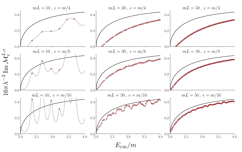
Figure 1: The estimator ${\rm Im}\,{\cal M}_{\rm c}^{L,\epsilon}$ from Eq. 87 (with $\Lambda=30m$) for various values of $mL$ and $\epsilon/m$. The volume increases from left to right and $\epsilon$ decreases from top to bottom. The desired ordered double limit is therefore approached by first extrapolating to the right and then down. Taking the limit in the incorrect order by decreasing $\epsilon/m$ at fixed $mL$ (going down a column) reveals contributions from individual finite-volume states, the values of which are indicated by the points.

Fig. 1 also gives the first indications of values for which the estimator in Eq. 87 is near the desired amplitude, suggesting that $mL\gtrsim 50$ is required for somewhat accurate results. This rather stringent guideline is relaxed significantly if extrapolations of $\epsilon/m\rightarrow 0$ are performed over a range of values at fixed $L$ which maintain $\epsilon L\gtrsim 4$. Such an extrapolation is illustrated in the left panel of Fig. 2, where the estimator from Eq. 87 is an apparently linear function of $\epsilon/m$ over the appropriate range. In the right panel of Fig. 2 we show the result of extrapolations for a wide range of volumes and energies. For a particular value of $L$ and $E_{\text{cm}}=2\sqrt{m^{2}+(2\pi\bm{n}/L)^{2}}$, the extrapolation is performed by comparing linear and quadratic fits in $\epsilon$ over the range $[4/L,\epsilon_{\text{max}}(p,L)]$. Here we have introduced $p^{2}=E_{\text{cm}}^{2}/4-m^{2}$ and have set

$$\epsilon_{\text{max}}(p,L)=\begin{cases}5/L&5/L<p\\ p&5/L\leq p<m\\ m&m\leq p\end{cases}\,.$$ (89)

This choice is motivated by the observation that the convergence is set by the branch point which is a distance $p$ from the desired on-shell pole. Rather than always taking $p$ as the upper limit, the maximum is truncated on either side by additional considerations: (i) the upper range should be well separated from $4/L$ and (ii) the particle mass sets a second scale that should not be exceeded. We stress that this approach is only a first step and a more detailed analysis is required in numerical applications.

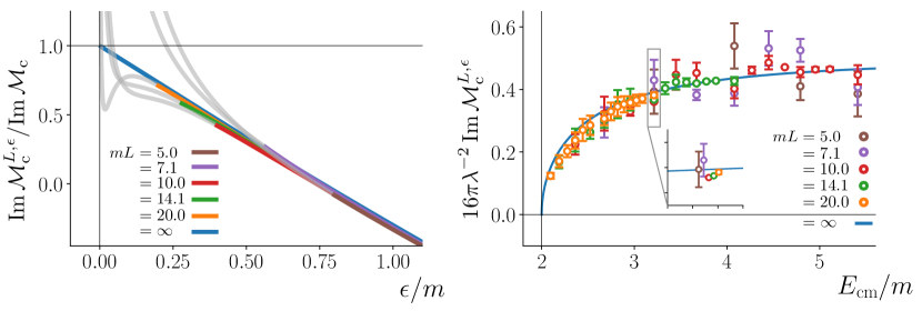
Figure 2: Extrapolations to $\epsilon=0$ at fixed $L$, keeping $\epsilon>4/L$. Left: The estimator from Eq. 87 for a set of volumes increasing in steps of $\sqrt{2}$ so that $E_{\text{cm}}$ is kept constant in physical units by adjusting the mode number $\bm{n}$, which is set to $\bm{n}^{2}=1$ at $mL=5$. The vertical axis is normalized to the correct infinite-volume, zero-$\epsilon$ value. For each $L$ the point $\epsilon=4/L$ is indicated by the transition from colored to gray. As the volume increases larger regions of the curve approach the $mL=\infty$ behavior, which is also shown. Right: Set of extrapolations $\epsilon\to 0$ at fixed $L$, as explained in the text. The inset shows the five points corresponding to the left panel. Here the central values are given by averaging the linear and quadratic fits in $\epsilon$ with a systematic uncertainty taken from their difference.

VI Conclusions and outlook

This work details a novel approach for determining scattering amplitudes from finite-volume Euclidean lattice field theory simulations. It is based on a relationship derived using the LSZ formalism between finite-volume spectral functions and arbitrary real-time infinite-volume scattering amplitudes.

Since the spectral function carries no information about the metric signature, it serves as a natural bridge between Euclidean and Minkowski time. The extraction of complex-valued scattering amplitudes requires the convolution of the spectral function with a particular complex smearing kernel which enforces the correct time ordering by implementing the $i\epsilon$-prescription. The amplitude is then recovered in three steps: (i) The limit $L\to\infty$ is saturated at fixed kernel-width $\epsilon$. (ii) A modified LSZ amputation is performed by multiplying with $\epsilon$ and dividing out operator overlaps. (iii) The limit $\epsilon\to 0^{+}$ is taken on the remaining, amputated object. The somewhat delicate interplay between the ordered double limit $\lim_{\epsilon\rightarrow 0^{+}}\lim_{L\rightarrow\infty}$, the analytic continuation between Euclidean and Minkowski time, the $i\epsilon$-prescription introduced by the smearing kernel, and the LSZ amputation procedure is illustrated for several examples in Sec. IV and perturbatively for two-to-two scattering in Sec. V.

Although the formalism underpinning this approach is conceptually straightforward, its implementation in lattice QCD simulations consists of several practical complications. First, connected higher $n$-point temporal correlation functions that are not typically calculated in lattice QCD are required, although zero-to-two processes such as the timelike pion form factor simply require conventional three-point correlators. In order to specify the momenta of each scatterer, $n-1$ of the hadron interpolators in these higher-order $n$-point functions must be projected onto a definite spatial momentum. The efficient evaluation of each Wick contraction, the number of which proliferates rapidly with $n$, likely presents a challenge. In addition to difficulties in calculating the $n$-point functions, the endcap functions from Eq. 19 are obtained by taking the asymptotic limit of time separations required to isolate the endcap states. The ubiquitous signal-to-noise problems plaguing standard lattice QCD calculations are therefore also relevant here.

Another practical difficulty concerns the determination of smeared spectral functions from Euclidean correlators. This effective replacement of decaying exponentials with $i\epsilon$-prescription pole factors is accomplished by the solution of an inverse problem. One possible strategy is a modification of the Backus-Gilbert approach, along the lines recently presented in Ref. Hansen:2019idp , in which the desired smearing kernel is treated as one of the inputs. Although the solution of such inverse problems is challenging, some potentially helpful prospects are discussed in Sec. III. These include the separate determinations of the real and imaginary parts of the spectral function in Eq. 26, the determination of contributions from individual finite-volume states in Eq. 25, the freedom of operator choice afforded by our amputation procedure, the prospect of using known properties of the $\epsilon$-dependence, and application of the unitarity cut formula of Eq. 28.

The final practical difficulty foreseen for this approach is that it requires larger volumes than those conventionally applied in lattice QCD simulations. While $m_{\pi}L\gtrsim 4$ is generally sufficient to suppress undesirable finite-volume effects in current calculations, the parameter $\epsilon$ introduces another infrared scale into the usual hierarchy. Specifically one must achieve $1/L\ll\epsilon\ll m_{\pi}$. Some indication of suitable values for $\epsilon L$ and $\epsilon/m_{\pi}$ is given in Sec. V, which suggests that $m_{\pi}L\approx 10-20$ may be sufficient.

For clarity, the formalism has been presented here for a single species of real scalar field. The straightforward generalization to complex arbitrary-spin fields with internal degrees of freedom is accomplished by replacing $\hat{\phi}(x)$ with the required interpolator and applying the standard modification to the LSZ formalism. Multiple species are also easily handled. To unambiguously select a desired in- or out-state, each individual field is placed on the mass shell of the desired particle. In contrast to the finite-volume Lüscher approach, additional spins and dynamical coupled scattering channels present no real difficulties here since the LSZ reduction is concerned with single-particle interpolators each of which are placed on shell individually. Particular initial and final states can therefore be unambiguously selected.

Another considerable advantage of this approach compared to Lüscher-type methods is its validity above arbitrary inelastic thresholds. This potentially extends the energy range for lattice QCD calculations of scattering amplitudes to encompass a number of interesting phenomenological applications. In particular, it provides a path by which many excited hadron resonances may be studied rigorously using lattice methods for the first time. Overall the outlook for the methods introduced here depends on the degree to which the practical difficulties discussed above are controlled. It is our view that the simplicity of the LSZ approach to lattice QCD calculations of scattering amplitudes justifies significant investment in overcoming these obstacles.

Acknowledgements: We acknowledge helpful conversations with M. Bruno, M. Della Morte, M. Lüscher, H. Meyer, and N. Tantalo. We also gratefully thank the Galileo Galilei Institute for Theoretical Physics and the Mainz Institute for Theoretical Physics for hospitality and support during completion of this work. Finally, we thank A. Francis and J. Ghiglieri, who, as the organizers of the CERN TH Institute “From Euclidean spectral densities to real-time physics”, provided an environment of insightful talks and discussion at the latter stages of the project.

Appendix A LSZ reduction for endcap functions

Here the LSZ reduction formula from Eq. 6 is proven for a general $m$-to-$n$ exclusive transition mediated by a local external current $\hat{J}(x)$. The less formal but more illustrative approach of Ref. Sterman:1994ce is employed. All of what follows is in infinite-volume Minkowski space.

Consider the endcap function defined in Eq. 5. We begin by reducing the rightmost field to isolate a two-particle in-state on the right endcap. Insert a complete set of two-particle in-states and examine the asymptotic contribution to the integral from the region $t_{2}<-t_{\rm c}<t_{3}$ with $t_{\rm c}>0$ taken arbitrarily large. This gives

$$\begin{split}\widetilde{F}^{J}_{\bm{p}_{m+n}\bm{p}_{1}}(q_{r+1},\dots,q_{2})&=\int\prod_{j=3}^{r+1}\left\{d^{4}x_{j}\,{\rm e}^{-iq_{j}\cdot x_{j}}\right\}\,\theta(t_{r+1}-t_{r})\cdots\theta(t_{4}-t_{3})\int d^{3}\bm{x}_{2}\int_{-\infty}^{-t_{\rm c}}dt_{2}\,{\rm e}^{-iq_{2}\cdot x_{2}}\,\\ &\times\int\!d\Gamma(\bm{k}_{1})d\Gamma(\bm{k}_{2})\ \langle\bm{p}_{m+n}|\hat{\phi}(x_{r+1})\cdots\hat{\phi}(x_{m+1})\,\hat{J}(0)\hat{\phi}(x_{m})\cdots\hat{\phi}(x_{3})|\bm{k}_{1}\bm{k}_{2}\rangle_{\rm in,c}\ {{}_{\rm in}\!\langle}\bm{k}_{1}\bm{k}_{2}|\hat{\phi}(x_{2})|\bm{p}_{1}\rangle+\cdots\,,\end{split}$$ (90)

where the ellipsis denotes contributions from ($k\neq 2$)-particle states and the remaining $t_{2}$-integration. In inserting the complete set of two-particle states the symmetry factor $1/2!$ has been neglected since it will be cancelled by a subsequent multiplicity.

Since we are interested only in the single-particle pole (in $q_{2}^{0})$ of Eq. 90 which occurs due to the $t_{2}\rightarrow-\infty$ contribution to the integral, the integrand may be replaced by its value in this limit. For this limiting value, the asymptotic formalism of Haag and Ruelle Haag ; Ruelle may be applied

$$\lim_{t_{2}\rightarrow-\infty}{{}_{\rm in}\langle}\bm{k}_{1}\bm{k}_{2}|\hat{\phi}(x_{2})|\bm{p}_{1}\rangle =\langle\bm{k}_{1}|\bm{p}_{1}\rangle\,\times\,\langle\bm{k}_{2}|\hat{\phi}(x_{2})|0\rangle\,,$$ (91)

$$=(2\pi)^{3}\,2E(\bm{p}_{1})\,\delta^{3}(\bm{k}_{1}-\bm{p}_{1})\,{\rm e}^{ik_{2}\cdot x_{2}}\,Z^{1/2}(\bm{k}_{2})\,,$$ (92)

where the multiplicity $2!$ mentioned above has been neglected. It should be noted that there is no analogous contribution in the $t_{2}\rightarrow\infty$ limit since the integrand is cut off by $\theta(t_{3}-t_{2})$.

The integral over $d^{3}\bm{x}_{2}$ results in $(2\pi)^{3}\delta^{3}(\bm{k}_{2}-\bm{p}_{2})$ which, when combined with $\delta^{3}(\bm{k}_{1}-\bm{p}_{1})$, selects a unique two-particle in-state

$$\widetilde{F}^{J}_{\bm{p}_{m+n}\bm{p}_{1}}(q_{r+1},\dots,q_{2})=\int\prod_{j=3}^{r+1}\left\{d^{4}x_{j}\,{\rm e}^{-iq_{j}\cdot x_{j}}\right\}\,\theta(t_{r+1}-t_{r})\cdots\theta(t_{4}-t_{3})\,\\ \times\frac{Z^{1/2}(\bm{p}_{2})}{2E(\bm{p}_{2})}\langle\bm{p}_{m+n}|\hat{\phi}(x_{r+1})\cdots\hat{\phi}(x_{m+1})\,\hat{J}(0)\hat{\phi}(x_{m})\cdots\hat{\phi}(x_{3})|\bm{p}_{1}\bm{p}_{2}\rangle_{\rm in,c}\int_{-\infty}^{-t_{\rm c}}dt_{2}\,{\rm e}^{-i(q_{2}^{0}-E(\bm{p}_{2})+i\epsilon)t_{2}}+\cdots\,.$$ (93)

where we have made the $i\epsilon$-prescription explicit in the $t_{2}$-dependence. The $t_{2}$-integral results in the expected pole factor

$$\int_{-\infty}^{-t_{\rm c}}dt_{2}\,{\rm e}^{-i(q_{2}^{0}-E(\bm{p}_{2})+i\epsilon)t_{2}}=\frac{i}{q_{2}^{0}-E(\bm{p}_{2})+i\epsilon}+\cdots\,,$$ (94)

where the ellipsis denotes subleading terms in the expansion of ${\rm e}^{i(q_{2}^{0}-E(\bm{p}_{2})+i\epsilon)t_{\rm c}}=1+\mathcal{O}\big{[}(q_{2}^{0}-E(\bm{p}_{2})+i\epsilon)\big{]}$.

The field $\hat{\phi}(x_{2})$ has thus been reduced into the right endcap isolating the two-particle in-state and corresponding pole factor from Eq. 94. Similarly, $\hat{\phi}(x_{r+1})$ may be reduced into the left endcap by inserting a complete set of two-particle out-states and examining the region $t_{r+1}>t_{\rm c}>t_{r}$. This process is subsequently applied to the left-most and right-most fields to reduce them into the left and right endcaps (respectively), achieving the desired result of Eq. 6.

References

- (1) L. Maiani and M. Testa, Final state interactions from Euclidean correlation functions, Phys. Lett. B245 (1990) 585–590.
- (2) M. Lüscher, Two particle states on a torus and their relation to the scattering matrix, Nucl. Phys. B354 (1991) 531–578.
- (3) K. Rummukainen and S. A. Gottlieb, Resonance scattering phase shifts on a nonrest frame lattice, Nucl. Phys. B450 (1995) 397–436, [hep-lat/9503028].
- (4) C. h. Kim, C. T. Sachrajda, and S. R. Sharpe, Finite-volume effects for two-hadron states in moving frames, Nucl. Phys. B727 (2005) 218–243, [hep-lat/0507006].
- (5) Z. Fu, Rummukainen-Gottlieb’s formula on two-particle system with different mass, Phys. Rev. D85 (2012) 014506, [arXiv:1110.0319].
- (6) S. He, X. Feng, and C. Liu, Two particle states and the S-matrix elements in multi-channel scattering, JHEP 07 (2005) 011, [hep-lat/0504019].
- (7) M. Lage, U.-G. Meißner, and A. Rusetsky, A Method to measure the antikaon-nucleon scattering length in lattice QCD, Phys. Lett. B681 (2009) 439–443, [arXiv:0905.0069].
- (8) V. Bernard, M. Lage, U. G. Meissner, and A. Rusetsky, Scalar mesons in a finite volume, JHEP 01 (2011) 019, [arXiv:1010.6018].
- (9) R. A. Briceno and Z. Davoudi, Moving multichannel systems in a finite volume with application to proton-proton fusion, Phys. Rev. D88 (2013), no. 9 094507, [arXiv:1204.1110].
- (10) M. T. Hansen and S. R. Sharpe, Multiple-channel generalization of Lellouch-Luscher formula, Phys. Rev. D86 (2012) 016007, [arXiv:1204.0826].
- (11) X. Feng, X. Li, and C. Liu, Two particle states in an asymmetric box and the elastic scattering phases, Phys. Rev. D70 (2004) 014505, [hep-lat/0404001].
- (12) M. Göckeler, R. Horsley, M. Lage, U. G. Meißner, P. E. L. Rakow, A. Rusetsky, G. Schierholz, and J. M. Zanotti, Scattering phases for meson and baryon resonances on general moving-frame lattices, Phys. Rev. D86 (2012) 094513, [arXiv:1206.4141].
- (13) R. A. Briceno, Two-particle multichannel systems in a finite volume with arbitrary spin, Phys. Rev. D89 (2014), no. 7 074507, [arXiv:1401.3312].
- (14) C. Morningstar, J. Bulava, B. Singha, R. Brett, J. Fallica, A. Hanlon, and B. Hörz, Estimating the two-particle -matrix for multiple partial waves and decay channels from finite-volume energies, Nucl. Phys. B924 (2017) 477–507, [arXiv:1707.05817].
- (15) L. Lellouch and M. Lüscher, Weak transition matrix elements from finite volume correlation functions, Commun. Math. Phys. 219 (2001) 31–44, [hep-lat/0003023].
- (16) C. J. D. Lin, G. Martinelli, C. T. Sachrajda, and M. Testa, K –> pi pi decays in a finite volume, Nucl. Phys. B619 (2001) 467–498, [hep-lat/0104006].
- (17) H. B. Meyer, Lattice QCD and the Timelike Pion Form Factor, Phys. Rev. Lett. 107 (2011) 072002, [arXiv:1105.1892].
- (18) R. A. Briceño, M. T. Hansen, and A. Walker-Loud, Multichannel 1 2 transition amplitudes in a finite volume, Phys. Rev. D91 (2015), no. 3 034501, [arXiv:1406.5965].
- (19) R. A. Briceño and M. T. Hansen, Multichannel 0 2 and 1 2 transition amplitudes for arbitrary spin particles in a finite volume, Phys. Rev. D92 (2015), no. 7 074509, [arXiv:1502.04314].
- (20) R. A. Briceño and M. T. Hansen, Relativistic, model-independent, multichannel transition amplitudes in a finite volume, Phys. Rev. D94 (2016), no. 1 013008, [arXiv:1509.08507].
- (21) A. Baroni, R. A. Briceño, M. T. Hansen, and F. G. Ortega-Gama, Form factors of two-hadron states from a covariant finite-volume formalism, arXiv:1812.10504.
- (22) R. A. Briceno and Z. Davoudi, Three-particle scattering amplitudes from a finite volume formalism, Phys. Rev. D87 (2013), no. 9 094507, [arXiv:1212.3398].
- (23) K. Polejaeva and A. Rusetsky, Three particles in a finite volume, Eur. Phys. J. A48 (2012) 67, [arXiv:1203.1241].
- (24) M. T. Hansen and S. R. Sharpe, Relativistic, model-independent, three-particle quantization condition, Phys. Rev. D90 (2014), no. 11 116003, [arXiv:1408.5933].
- (25) U.-G. Meißner, G. Rios, and A. Rusetsky, Spectrum of three-body bound states in a finite volume, Phys. Rev. Lett. 114 (2015), no. 9 091602, [arXiv:1412.4969]. [Erratum: Phys. Rev. Lett.117,no.6,069902(2016)].
- (26) M. T. Hansen and S. R. Sharpe, Expressing the three-particle finite-volume spectrum in terms of the three-to-three scattering amplitude, Phys. Rev. D92 (2015), no. 11 114509, [arXiv:1504.04248].
- (27) R. A. Briceño, M. T. Hansen, and S. R. Sharpe, Relating the finite-volume spectrum and the two-and-three-particle matrix for relativistic systems of identical scalar particles, Phys. Rev. D95 (2017), no. 7 074510, [arXiv:1701.07465].
- (28) M. Mai and M. Döring, Three-body Unitarity in the Finite Volume, Eur. Phys. J. A53 (2017), no. 12 240, [arXiv:1709.08222].
- (29) H.-W. Hammer, J.-Y. Pang, and A. Rusetsky, Three-particle quantization condition in a finite volume: 1. The role of the three-particle force, JHEP 09 (2017) 109, [arXiv:1706.07700].
- (30) H. W. Hammer, J. Y. Pang, and A. Rusetsky, Three particle quantization condition in a finite volume: 2. general formalism and the analysis of data, JHEP 10 (2017) 115, [arXiv:1707.02176].
- (31) M. Döring, H. W. Hammer, M. Mai, J. Y. Pang, Â. A. Rusetsky, and J. Wu, Three-body spectrum in a finite volume: the role of cubic symmetry, Phys. Rev. D97 (2018), no. 11 114508, [arXiv:1802.03362].
- (32) R. A. Briceño, M. T. Hansen, and S. R. Sharpe, Three-particle systems with resonant subprocesses in a finite volume, arXiv:1810.01429.
- (33) F. Romero-López, A. Rusetsky, and C. Urbach, Two- and three-body interactions in theory from lattice simulations, Eur. Phys. J. C78 (2018), no. 10 846, [arXiv:1806.02367].
- (34) M. T. Hansen and S. R. Sharpe, Lattice QCD and Three-particle Decays of Resonances, arXiv:1901.00483.
- (35) T. D. Blanton, F. Romero-López, and S. R. Sharpe, Implementing the three-particle quantization condition including higher partial waves, arXiv:1901.07095.
- (36) C. Andersen, J. Bulava, B. Hörz, and C. Morningstar, The pion-pion scattering amplitude and timelike pion form factor from lattice QCD, Nucl. Phys. B939 (2019) 145–173, [arXiv:1808.05007].
- (37) A. Woss, C. E. Thomas, J. J. Dudek, R. G. Edwards, and D. J. Wilson, Dynamically-coupled partial-waves in isospin-2 scattering from lattice QCD, JHEP 07 (2018) 043, [arXiv:1802.05580].
- (38) C. Alexandrou, L. Leskovec, S. Meinel, J. Negele, S. Paul, M. Petschlies, A. Pochinsky, G. Rendon, and S. Syritsyn, -wave scattering and the resonance from lattice QCD, Phys. Rev. D96 (2017), no. 3 034525, [arXiv:1704.05439].
- (39) J. Bulava, B. Fahy, B. Hörz, K. J. Juge, C. Morningstar, and C. H. Wong, and scattering phase shifts from lattice QCD, Nucl. Phys. B910 (2016) 842–867, [arXiv:1604.05593].
- (40) Z. Fu and L. Wang, Studying the resonance parameters with staggered fermions, Phys. Rev. D94 (2016), no. 3 034505, [arXiv:1608.07478].
- (41) D. Guo, A. Alexandru, R. Molina, and M. Döring, resonance parameters from lattice QCD, Phys. Rev. D94 (2016), no. 3 034501, [arXiv:1605.03993].
- (42) R. A. Briceno, J. J. Dudek, R. G. Edwards, and D. J. Wilson, Isoscalar scattering and the meson resonance from QCD, Phys. Rev. Lett. 118 (2017), no. 2 022002, [arXiv:1607.05900].
- (43) D. J. Wilson, R. A. Briceno, J. J. Dudek, R. G. Edwards, and C. E. Thomas, Coupled scattering in -wave and the resonance from lattice QCD, Phys. Rev. D92 (2015), no. 9 094502, [arXiv:1507.02599].
- (44) X. Feng, S. Aoki, S. Hashimoto, and T. Kaneko, Timelike pion form factor in lattice QCD, Phys. Rev. D91 (2015), no. 5 054504, [arXiv:1412.6319].
- (45) Hadron Spectrum Collaboration, J. J. Dudek, R. G. Edwards, and C. E. Thomas, Energy dependence of the resonance in elastic scattering from lattice QCD, Phys.Rev. D87 (2013), no. 3 034505, [arXiv:1212.0830].
- (46) C. Pelissier and A. Alexandru, Resonance parameters of the rho-meson from asymmetrical lattices, Phys. Rev. D87 (2013), no. 1 014503, [arXiv:1211.0092].
- (47) CS Collaboration, S. Aoki et al., Meson Decay in 2+1 Flavor Lattice QCD, Phys. Rev. D84 (2011) 094505, [arXiv:1106.5365].
- (48) C. B. Lang, D. Mohler, S. Prelovsek, and M. Vidmar, Coupled channel analysis of the meson decay in lattice QCD, Phys. Rev. D84 (2011), no. 5 054503, [arXiv:1105.5636]. [Erratum: Phys. Rev.D89,no.5,059903(2014)].
- (49) X. Feng, K. Jansen, and D. B. Renner, Resonance Parameters of the -Meson from Lattice QCD, Phys. Rev. D83 (2011) 094505, [arXiv:1011.5288].
- (50) C. W. Andersen, J. Bulava, B. Hörz, and C. Morningstar, Elastic , -wave nucleon-pion scattering amplitude and the (1232) resonance from Nf=2+1 lattice QCD, Phys. Rev. D97 (2018), no. 1 014506, [arXiv:1710.01557].
- (51) C. B. Lang, L. Leskovec, M. Padmanath, and S. Prelovsek, Pion-nucleon scattering in the Roper channel from lattice QCD, Phys. Rev. D95 (2017), no. 1 014510, [arXiv:1610.01422].
- (52) C. Lang and V. Verduci, Scattering in the negative parity channel in lattice QCD, Phys.Rev. D87 (2013), no. 5 054502, [arXiv:1212.5055].
- (53) W. Detmold and A. Nicholson, Low energy scattering phase shifts for meson-baryon systems, Phys. Rev. D93 (2016), no. 11 114511, [arXiv:1511.02275].
- (54) E. Berkowitz, T. Kurth, A. Nicholson, B. Joo, E. Rinaldi, M. Strother, P. M. Vranas, and A. Walker-Loud, Two-Nucleon Higher Partial-Wave Scattering from Lattice QCD, Phys. Lett. B765 (2017) 285–292, [arXiv:1508.00886].
- (55) K. Orginos, A. Parreno, M. J. Savage, S. R. Beane, E. Chang, and W. Detmold, Two nucleon systems at from lattice QCD, Phys. Rev. D92 (2015), no. 11 114512, [arXiv:1508.07583].
- (56) R. A. Briceno, J. J. Dudek, R. G. Edwards, and D. J. Wilson, Isoscalar scattering and the mesons from QCD, Phys. Rev. D97 (2018), no. 5 054513, [arXiv:1708.06667].
- (57) G. Moir, M. Peardon, S. M. Ryan, C. E. Thomas, and D. J. Wilson, Coupled-Channel , and Scattering from Lattice QCD, JHEP 10 (2016) 011, [arXiv:1607.07093].
- (58) Hadron Spectrum Collaboration, J. J. Dudek, R. G. Edwards, and D. J. Wilson, An resonance in strongly coupled , scattering from lattice QCD, Phys. Rev. D93 (2016), no. 9 094506, [arXiv:1602.05122].
- (59) D. J. Wilson, J. J. Dudek, R. G. Edwards, and C. E. Thomas, Resonances in coupled scattering from lattice QCD, Phys. Rev. D91 (2015), no. 5 054008, [arXiv:1411.2004].
- (60) D. Mohler, C. B. Lang, L. Leskovec, S. Prelovsek, and R. M. Woloshyn, Meson and -Meson-Kaon Scattering from Lattice QCD, Phys. Rev. Lett. 111 (2013), no. 22 222001, [arXiv:1308.3175].
- (61) C. Alexandrou, L. Leskovec, S. Meinel, J. Negele, S. Paul, M. Petschlies, A. Pochinsky, G. Rendon, and S. Syritsyn, transition and the radiative decay width from lattice QCD, Phys. Rev. D98 (2018), no. 7 074502, [arXiv:1807.08357].
- (62) R. A. Briceño, J. J. Dudek, R. G. Edwards, C. J. Shultz, C. E. Thomas, and D. J. Wilson, The amplitude and the resonant transition from lattice QCD, Phys. Rev. D93 (2016), no. 11 114508, [arXiv:1604.03530].
- (63) F. Romero-López, A. Rusetsky, and C. Urbach, Vector particle scattering on the lattice, Phys. Rev. D98 (2018), no. 1 014503, [arXiv:1802.03458].
- (64) S. L. Olsen, T. Skwarnicki, and D. Zieminska, Nonstandard heavy mesons and baryons: Experimental evidence, Rev. Mod. Phys. 90 (2018), no. 1 015003, [arXiv:1708.04012].
- (65) F.-K. Guo, C. Hanhart, U.-G. Meißner, Q. Wang, Q. Zhao, and B.-S. Zou, Hadronic molecules, Rev. Mod. Phys. 90 (2018), no. 1 015004, [arXiv:1705.00141].
- (66) R. F. Lebed, R. E. Mitchell, and E. S. Swanson, Heavy-Quark QCD Exotica, Prog. Part. Nucl. Phys. 93 (2017) 143–194, [arXiv:1610.04528].
- (67) A. Esposito, A. Pilloni, and A. D. Polosa, Multiquark Resonances, Phys. Rept. 668 (2016) 1–97, [arXiv:1611.07920].
- (68) H.-X. Chen, W. Chen, X. Liu, and S.-L. Zhu, The hidden-charm pentaquark and tetraquark states, Phys. Rept. 639 (2016) 1–121, [arXiv:1601.02092].
- (69) R. Gothe, Y. Ilieva, V. Mokeev, E. Santopinto, and S. Strauch, eds., Proceedings, 11th International Workshop on the Physics of Excited Nucleons (NSTAR 2017), vol. 59, 2018.
- (70) P. A. Boyle, Machines and Algorithms, PoS LATTICE2016 (2017) 013.
- (71) M. Lüscher, Stochastic locality and master-field simulations of very large lattices, EPJ Web Conf. 175 (2018) 01002, [arXiv:1707.09758].
- (72) M. Cè, L. Giusti, and S. Schaefer, A local factorization of the fermion determinant in lattice QCD, Phys. Rev. D95 (2017), no. 3 034503, [arXiv:1609.02419].
- (73) M. Cè, L. Giusti, and S. Schaefer, Domain decomposition, multi-level integration and exponential noise reduction in lattice QCD, Phys. Rev. D93 (2016), no. 9 094507, [arXiv:1601.04587].
- (74) M. T. Hansen, H. B. Meyer, and D. Robaina, From deep inelastic scattering to heavy-flavor semileptonic decays: Total rates into multihadron final states from lattice QCD, Phys. Rev. D96 (2017), no. 9 094513, [arXiv:1704.08993].
- (75) G. Backus and F. Gilbert, The resolving power of gross earth data, Geophysical Journal International 16 (1968), no. 2 169–205.
- (76) G. Backus and F. Gilbert, Uniqueness in the inversion of inaccurate gross earth data, Philosophical Transactions of the Royal Society of London A: Mathematical, Physical and Engineering Sciences 266 (1970), no. 1173 123–192, [http://rsta.royalsocietypublishing.org/content/266/1173/123.full.pdf].
- (77) K.-F. Liu and S.-J. Dong, Origin of difference between anti-d and anti-u partons in the nucleon, Phys. Rev. Lett. 72 (1994) 1790–1793, [hep-ph/9306299].
- (78) K.-F. Liu, Parton Distribution Function from the Hadronic Tensor on the Lattice, PoS LATTICE2015 (2016) 115, [arXiv:1603.07352].
- (79) K.-F. Liu, Evolution Equations for Connected and Disconnected Sea Partons, arXiv:1703.04690.
- (80) S. Hashimoto, Inclusive semi-leptonic B meson decay structure functions from lattice QCD, PTEP 2017 (2017), no. 5 053B03, [arXiv:1703.01881].
- (81) D. Agadjanov, M. Döring, M. Mai, U.-G. Meißner, and A. Rusetsky, The Optical Potential on the Lattice, JHEP 06 (2016) 043, [arXiv:1603.07205].
- (82) J. C. A. Barata and K. Fredenhagen, Particle scattering in Euclidean lattice field theories, Commun. Math. Phys. 138 (1991) 507–520.
- (83) H. Lehmann, K. Symanzik, and W. Zimmermann, Zur formulierung quantisierter feldtheorien, Il Nuovo Cimento (1955-1965) 1 (Jan, 1955) 205–225.
- (84) R. Haag, Quantum Field Theories with Composite Particles and Asymptotic Conditions, Physical Review 112 (Oct., 1958) 669–673.
- (85) D. Ruelle, On the asymptotic condition in quantum field theory, Helv. Phys. Acta 35 (01, 1962).
- (86) M. Hansen, A. Lupo, and N. Tantalo, On the extraction of spectral densities from lattice correlators, arXiv:1903.06476.
- (87) M. Asakawa, T. Hatsuda, and Y. Nakahara, Maximum entropy analysis of the spectral functions in lattice QCD, Prog. Part. Nucl. Phys. 46 (2001) 459–508, [hep-lat/0011040].
- (88) B. B. Brandt, A. Francis, H. B. Meyer, and D. Robaina, Pion quasiparticle in the low-temperature phase of QCD, Phys. Rev. D92 (2015), no. 9 094510, [arXiv:1506.05732].
- (89) C. Michael, Adjoint Sources in Lattice Gauge Theory, Nucl. Phys. B259 (1985) 58–76.
- (90) M. Luscher and U. Wolff, How to Calculate the Elastic Scattering Matrix in Two-dimensional Quantum Field Theories by Numerical Simulation, Nucl. Phys. B339 (1990) 222–252.
- (91) B. Blossier, M. Della Morte, G. von Hippel, T. Mendes, and R. Sommer, On the generalized eigenvalue method for energies and matrix elements in lattice field theory, JHEP 04 (2009) 094, [arXiv:0902.1265].
- (92) M. Della Morte et al., A lattice calculation of the hadronic vacuum polarization contribution to , EPJ Web Conf. 175 (2018) 06031, [arXiv:1710.10072].
- (93) TOTEM Collaboration, G. Antchev et al., First measurement of elastic, inelastic and total cross-section at TeV by TOTEM and overview of cross-section data at LHC energies, Eur. Phys. J. C79 (2019), no. 2 103, [arXiv:1712.06153].
- (94) G. F. Sterman, An Introduction to quantum field theory. Cambridge University Press, 1993.