Multifractality in random networks with power–law decaying bond strengths
Abstract
In this paper we demonstrate numerically that random networks whose adjacency matrices are represented by a diluted version of the Power–Law Banded Random Matrix (PBRM) model have multifractal eigenfunctions. The PBRM model describes one–dimensional samples with random long–range bonds. The bond strengths of the model, which decay as a power–law, are tuned by the parameter as ; while the sparsity is driven by the average network connectivity : for the vertices in the network are isolated and for the network is fully connected and the PBRM model is recovered. Though it is known that the PBRM model has multifractal eigenfunctions at the critical value , we clearly show [from the scaling of the relative fluctuation of the participation number as well as the scaling of the probability distribution functions ] the existence of the critical value for . Moreover, we characterise the multifractality of the eigenfunctions of our random network model by the use of the corresponding multifractal dimensions , that we compute from the finite network-size scaling of the typical eigenfunction participation numbers .
pacs:
64.60.Aq 89.75.HcI Introduction
Fractality is related to phase transitions in critical phenomena observed in several complex systems Stanley71 ; Vicsek92 . Blood vessels, proteins, ocean waves, animal collaboration patterns, and earthquakes exhibit fractality Mandelbrot1983 ; Bunde013 . Fractality can also be understood as a signature of the organisation and structure of complex systems, which is far from random or regular Costa011 . Moreover, the structure of complex systems can be mapped to networks, whose structure SHM05 and evolution Song06 exhibit fractal properties.
Fractality in networks has been extensively discussed from several perspectives SHM05 ; Costa07 . These studies have focused on the structural characterisation of fractal networks SHM05 ; Song06 or networks expressly constructed as fractal objects (deterministic or disordered, e.g. see MB11 ; GSKK06 ; CR10 ; LYZ14 ; STM17 ). In this respect some algorithms have been developed and applied to compute the fractal dimension of complex networks, see for example SHM05 ; GSKK06 ; KGS07 ; SGHM07 ; S07 ; LKBH11 ; FY11 ; LYA15 and references therein. On the other hand, given a fractal network, there is plenty of works devoted to the signatures of the fractality on the network properties. Among them we can mention the underlying tree structure or skeleton GSKK06 ; KGS07 as well as dynamical and transport properties, see for example MB11 ; Y02 ; GSH07 ; ZZTC08 ; TL99 ; ZYG11 ; KDM15 .
Here, we approach an alternative but close-related subject: We explore the fractality of the eigenfunctions of the adjacency matrices of a random network model. Moreover, we demonstrate that imposing power–law correlations, i.e. with , on a random network model of the Erdös-Rényi–type produces multifractal eigenfunctions.
Therefore, in the following section we first review the Power–Law Banded Random Matrix (PBRM) model; a random matrix model used to study the Anderson metal-to-insulator phase transition, which presents multifractal eigenfunctions at the transition point. Then, we introduce the diluted PBRM (dPBRM) model as an ensemble of adjacency matrices of random networks of the Erdös-Rényi–type. Using scaling arguments, in Sect. III we show that the dPBRM model also exhibits a metal-to-insulator phase transition where the corresponding eigenfunctions are multifractal objects. Finally, in Sect. IV we draw our conclusions.
II The random network model
II.1 The Power–Law Banded Random Matrix model
The Power–Law Banded Random Matrix (PBRM) model MFDQS96 is represented by real symmetric matrices whose elements are statistically independent random variables drawn from a normal distribution with zero mean, , and a variance given by
| (1) |
where and are the model parameters. The PBRM model has been used to describe one–dimensional tight-binding wires of length with random long–range hoppings. In Eq. (1) the PBRM model is in its periodic version; i.e., the one–dimensional wire is in a ring geometry. Theoretical considerations MFDQS96 ; EM08 ; Mirlin00 ; KT00 and detailed numerical investigations EM08 ; EM00b ; V00 ; V02 have verified that the PBRM model undergoes a transition at , i.e., from localized eigenfunctions for to delocalized eigenfunctions for . This transition shows key features of the disorder driven Anderson metal-insulator transition EM08 ; MKV05 ; APB09 ; MAV14 , including multifractality of eigenfunctions and non-trivial spectral statistics. Thus the PBRM model possesses a line of critical points at . By tuning the parameter , from to , the eigenfunctions cross over from the strong multifractality () which corresponds to localized–like or insulator–like eigenfunctions to weak multifractality (), showing rather extended, i.e., metallic–like eigenfunctions EM08 ; Mirlin00 . Here, are the eigenfunction’s multifractal dimensions (to be defined in Sect. III). At the true Anderson transition in or at the integer quantum–Hall transition in the eigenfunctions belong to the weakly multifractal regime, i.e., ; it is relevant to note that the PBRM model allows for investigations without such a limitation.
II.2 The diluted Power–Law Banded Random Matrix model
Here we introduce the diluted PBRM (dPBRM) model as follows: Starting with the PBRM model, we randomly set off-diagonal matrix elements to zero such that the sparsity (i.e., the average network connectivity) is defined as the fraction of the independent non-vanishing off-diagonal matrix elements. According to this definition, a diagonal random matrix is obtained for , whereas the PBRM model is recovered when .
The Erdös-Rényi adjacency matrix is considered as a mask to define the nonzero matrix elements of our dPBRM model. Hence, notice that the dPBRM model of size works as an ensemble of adjacency matrices of Erdös-Rényi–type networks formed by vertices. For such networks we allow self-edges and further consider all edges to have random strengths; however, notice that the random strengths are power–law modulated, see Eq. (1).
The power–law correlations of the dPBRM model are tuned by the parameter as , see Eq. (1). Notice that for the vertices in the network become isolated since ; while for the dPBRM model reproduces the Erdös-Rényi random network model with maximal disorder (see Refs. MAM13 ; MAM15 ; GAC18 ). However, here we set such that we recover the PBRM model at criticality (i.e., the PBRM model having multifractal eigenfunctions) when . Moreover, without loss of generality, we will set the effective bandwidth of the dPBRM model to unity; that is, we use the bandwidth that produces multifractal eigenfunctions with intermediate fractality, , in the PBRM model. Here is the correlation dimension of the eigenfunctions.
Note that another diluted version of the PBRM model was reported in Refs. LL01 ; SAML08 ; AML08 in studies of quantum percolation.
In the following Section we demonstrate that the eigenfunctions of the dPBRM model are multifractal objects. Besides, we share the implementation and analyses of the reported model online 111Code available at https://github.com/didiervega/RandomMatrix, for easier reproducibility.
III Network Eigenfunction Multifractality
Given an eigenfunction it is a common practice (in random matrix models and complex Hamiltonian systems) to characterise its complexity by the use of the generalised participation numbers
| (2) |
where is the corresponding matrix size. In particular, the participation number is roughly equal to the number of principal eigenfunction components, and therefore, is a widely accepted measure of the extension of the eigenfunction in a given basis. Participation numbers and also inverse participation ratios (i.e., ) have been already used to characterise the eigenfunctions of the adjacency matrices of random network models (see some examples in Refs. F01 ; MPV07 ; CAS08 ; GGS09 ; JZL11 ; S12 ; PMCM13 ; MZN14 ).
In the context of random matrix models showing the metal-to-insulator phase transition, such as the PBRM model, it is well established that the distribution functions of the inverse participation ratios are scale invariant at the transition point EM00 where the eigenfunctions are multifractal objects (see also V02 ). The PBRM model with is at criticality, however, introducing the sparsity may relocate the metal-to-insulator transition point. Therefore, before talking about multifractality of eigenfunctions for the dPBRM model we first have to be sure that the system is at criticality. Thus, to search out the critical points of the dPBRM model with we use the relative fluctuation (the ratio of the standard deviation to the mean value) of the participation number ,
| (3) |
Indeed, this quantity has been used to locate the metal-to-insulator transition point in random SAML08 and non-random MMD04 long–range hopping models.
In the following, we use exact numerical diagonalisation to obtain the eigenfunctions of the adjacency matrices of large ensembles of random networks, represented by the dPBRM model (characterized by and ).
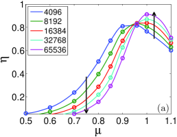
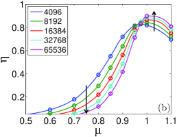
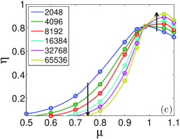
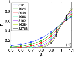
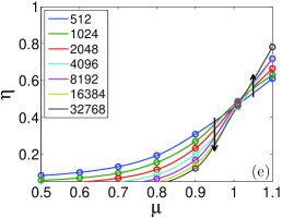
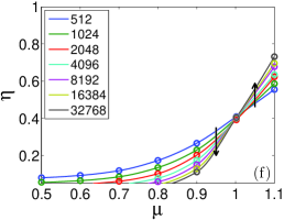
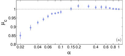
In Fig. 1 we present the curves of vs. for the dPBRM model with sparsity . For a given value of the sparsity we show curves corresponding to different (exponentially growing) network sizes. For all the values of we consider here, , we observe two opposing behaviours: When [] the quantity decreases [increases] for increasing [decreasing] network size . Moreover, we observe that curves for different have a fixed point at , revealing the invariance of and therefore the existence of a metal-to-insulator transition point at . Then, in Fig. 2(a) we plot vs. . From this figure we can see that: for moderate sparsity, i.e., , ; while for relatively strong sparsity, i.e, , decreases for decreasing .
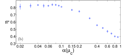
As complementary information, in Fig. 2(b) we report the values of the relative fluctuation of the participation number that we found at . As for , here we also observe two different behaviours for : while it decreases for increasing when ; it is interesting to note that is approximately constant () for relatively strong sparsity, .
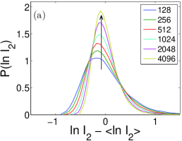
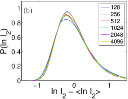
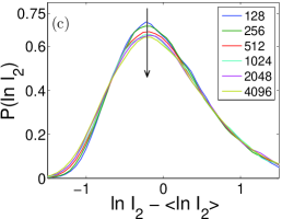
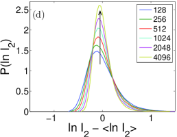


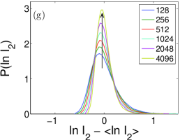
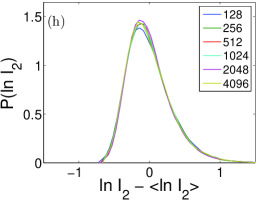
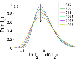
We stress that from Fig. 1 we have located the critical points for different values of (reported in Fig. 2) by the use of the invariance of the relative fluctuation of the participation number . Moreover, we can further verify the existence of from the invariance of the probability distribution function (PDF) of itself (see for example EM00 ; V02 ). Thus, in Fig. 3 we show PDFs of the participation number for the dPBRM model with sparsity , 0.6, and . For each we have selected three values of : , , and . As well as for , here we identify two behaviours for depending on whether or : When [] the histograms of are narrower [wider] the larger [smaller] the network size. While, as predicted EM00 ; V02 , is invariant at and falls on top of a universal PDF when plotted as a function of . We merely want to comment that for small network sizes, , at we observe that evolves as a function of ; which is a finite size effect. Indeed, as clearly seen in Fig. 3, is already invariant for .
Once we know the position of for the dPBRM model, we can characterise the multifractality of the corresponding eigenfunctions through the eigenfunction multifractal dimensions , which are defined by the scaling of the typical participation numbers
| (4) |
as a function of :
| (5) |
The multifractal dimensions can also be extracted from the scaling of the average participation numbers, , however here we choose to use typical participation numbers. We recall that for strongly localized eigenfunctions the corresponding does not scale with the system size: and for all . This situation corresponds to an insulating regime. While extended eigenfunctions always feel the entire system. Thus, a signature of the metallic regime is given by and . Moreover, multifractal eigenfunctions should be described by the series of , which are nonlinear functions of the index .
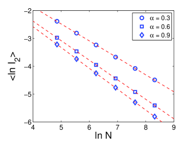
We extract the multifractal dimensions from the linear fit of the logarithm of the typical participation numbers versus the logarithm of (see Eq. (5)). We use , . The average was performed over eigenfunctions with eigenvalues around the band centre with realisations of our dPBRM model. As examples, in Fig. 4 we present the scalings of vs. for selected values of sparsity. Therefore, the correlation dimension is extracted from the linear fits to the data (see dashed lines). We note the remarkably clean linear scaling of vs. .
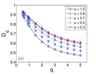
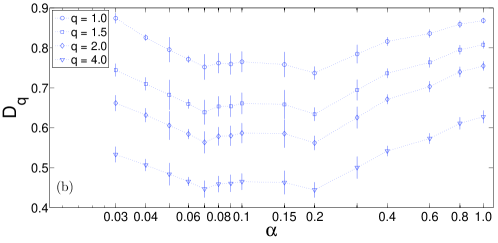
Finally, in Fig. 5(a) we report the multifractal dimensions as a function of for the dPBRM model with selected values of (to avoid figure saturation). The nonlinearity of the curves vs. is the signature of the multifractality of eigenfunctions of our network model. Also, as a reference, in Fig. 5(a) we include the values of for the PBRM model (i.e. the values of for the dPBRM model with ). Additionally, in Fig. 5(b) we show vs. for selected values of , in particular we include the information dimension and the correlation dimension . From this figure we observe two behaviours: an initial decrease of for decreasing , for relatively large values of (); while, remarkably, the further decreasing of (i.e., ) makes the multifractality of the eigenfunctions of the dPBRM model to grow to values close to those for weak sparsity.
IV Discussion and conclusions
In this paper we consider random networks whose adjacency matrices are represented by a sparse version of the Power–Law Banded Random Matrix (PBRM) model, therefore having a power–law structure, , tuned by the parameter (see Eq. (1)). We call this random network model the diluted PBRM (dPBRM) model. We would like to emphasise that the dPBRM model belongs to the same universality class than the PBRM model, as discussed in CRBD17 where more general long-range quantum hopping models in one-dimension have been studied.
The sparsity of the dPBRM model is driven by the average network connectivity : for the vertices in the network are isolated and for the network is fully connected. Notice that the original PBRM model is recovered for , which is known to have multifractal eigenfunctions at the critical value where a metal-to-insulator phase transition takes place. Here, we show that the dPBRM model exhibits a critical value for , as reported in Fig. 2. Moreover, we found that for ; while for relatively strong sparsity, or (since , where is the average degree), decreases for decreasing .
In addition, we demonstrate the multifractality of the eigenfunctions of our random network model at by the calculation of the corresponding multifractal dimensions . Indeed, we observed from Fig. 5 that the multifractality of the eigenfunctions of the dPBRM model can be effectively tuned by the average network connectivity .
We emphasize that the calculation of from the finite network-size scaling of the typical eigenfunction participation numbers, see Eq. (5), is equivalent to a standard box covering algorithm (where the network size works as the box size). However, due to the normalised nature of the eigenfunctions, the scaling of vs. is very stable, as clearly shown in Fig. 4, providing quite precise values of multifractal dimensions.
Our approach may be used to investigate the multifractality of eigenfunctions in other random network models. Indeed, similar studies have been already performed to explore the multifractality of eigenfunctions of the Anderson model on Cayley trees (AMCT) STM17 ; MG11 ; TM16 and random graphs GGG17 . It is relevant to stress that there are three important differences between the network model studied here and the AMCT studied in Refs. STM17 ; MG11 : (i) Cayley trees have a fixed degree (the AMCT in STM17 ; MG11 is characterized by ), while due to the random-network nature of the dPBRM model the degree is defined as an average quantity here. (ii) The dPBRM model represents networks with randomly-weighted bond strengths between vertices, while the AMCT in STM17 ; MG11 is defined as a network with constant bond strengths. (iii) The dPBRM model possesses an infinite line of critical points characterized by the parameter (that we did not examine here since we fixed in Eq. (1) as a representative case), whereas the AMCT has a single critical point for a given on-site disorder strength. Thus, even though it may be expected that the dPBRM with should show similar properties than the AMCT in STM17 ; MG11 , this must be properly verified, given the differences between both models. Moreover, inspired by MG11 ; TM19 it should also be interesting to explore the eigenfunction statistics of the dPBRM model off criticality, i.e., in Eq. (1).
The relation between the fractality of networks (in networks specifically constructed as deterministic or disordered fractal objects) and the (possible) fractality of the eigenfunctions of the corresponding adjacency matrix is also another important subject to be explored.
We would like to add that the dPBRM model, when interpreted as a model for one-dimensional quantum chains with long–range interactions, has characteristics proper of models currently used in the study of excitation transport NP18 : disorder and power–law decaying bond strengths. Furthermore, these characteristics can presumably be implemented and tuned in state-of-the-art ion-chain experiments; thus the dPBRM model may find applications related to quantum transport with high efficiencies NP18 .
Acknowledgements.
Research carried out using the computational resources of the Center for Mathematical Sciences Applied to Industry (CeMEAI) funded by FAPESP (Fundação de Amparo à Pesquisa do Estado de São Paulo, Grant No. 2013/07375-0). J.A.M.-B. acknowledges support from VIEP-BUAP (Grant No. MEBJ-EXC18-G), Fondo Institucional PIFCA (Grant No. BUAP-CA-169), and CONACyT (Grant No. CB-2013/220624). F.A.R. acknowledges CNPq (Grant No. 305940/2010-4) and FAPESP (Grant No. 13/26416-9). D.A.VO. acknowledges CNPq (Grant 140688/2013-7) and FAPESP (Grant No. 2016/23698-1).References
- [1] T. Vicsek, Fractal growth phenomena, World Scientific (1992).
- [2] H. E. Stanley, Introduction to phase transitions and critical phenomena, Oxford University Press (1971).
- [3] B. B. Mandelbrot, The fractal geometry of nature, Macmillan (1983).
- [4] A. Bunde and S. Havlin, Fractals in science, Springer (2013).
- [5] L. da F. Costa, O. N. Oliveira Jr., G. Travieso, F. A. Rodrigues, P. R. Villas Boas, L. Antiqueira, M. P. Viana, and L. R. C. Rocha, Advances in Physics 60, 3 (2011).
- [6] C. Song, S. Havlin, and H. A. Makse, Nature (London) 433, 392 (2005).
- [7] S. Chaoming, S. Havlin, and A. H. Makse, Nature Physics 2, 4 (2006).
- [8] L. da F. Costa, F. A. Rodrigues, G. Travieso, and P. R. Villas Boas, Advances in Physics 56, 1 (2007).
- [9] O. Mülken and A. Blumen, Phys. Rep. 502, 37 (2011).
- [10] K.-I. Goh, G. Salvi, B. Kahng, and D. Kim, Phys. Rev. Lett. 96, 018701 (2006).
- [11] T. Carletti and S. Righi, Physica A 389, 2134 (2010).
- [12] B.-G. Li, Z.-G. Yu, and Y. Zhou, J. Stat. Mech. P02020 (2014).
- [13] M. Sonner, K. S. Tikhonov, and A. D. Mirlin, Phys. Rev. B 96, 214204 (2017).
- [14] J. S. Kim, K.-I. Goh, G. Salvi, E. Oh, B. Kahng, and D. Kim, Phys. Rev. E 75, 016110 (2007).
- [15] C. Song, L. K. Gallos, S. Havlin, and H. A. Makse, J. Stat. Mech. P03006 (2007).
- [16] O. Shanker, Mod. Phys. Lett. B 21, 321 (2007).
- [17] D. Li, K. Kosmidis, A. Bunde, and S. Havlin, Nature Physics 7, 481 (2011).
- [18] S. Furuya and K. Yakubo, Phys. Rev. E 84, 036118 (2011).
- [19] J.-L. Liu, Z.-G. Yu, and V. Anh, Chaos 25, 023103 (2015).
- [20] A. V. N. C. Teixeira and P. Licinio, Europhys. Lett. 45, 162 (1999).
- [21] X.-S. Yang, Chaos Solitons Fractals 13 215 (2002).
- [22] L. K. Gallos, C. Song, S. Havlin, and H. A. Makse, Proc. Natl. Acad. Sci. 104, 7746 (2007).
- [23] Z. Zhang, S. Zhou, Z. Tao, and G. Chen, J. Stat. Mech. P09008 (2008).
- [24] Z. Zhang, Y. Yang, S. Gao, Eur. Phys. J. B 84, 331 (2011).
- [25] N. Kulvelis, M. Dolgushev, O. Mülken, Phys. Rev. Lett. 115, 120602 (2015).
- [26] A. D. Mirlin, Y. V. Fyodorov, F.-M. Dittes, J. Quezada, and T. H. Seligman, Phys. Rev. E 54, 3221 (1996).
- [27] F. Evers and A. D. Mirlin, Rev. Mod. Phys. 80, 1355 (2008).
- [28] A. D. Mirlin, Phys. Rep. 326, 259 (2000).
- [29] V. E. Kravtsov and K. A. Muttalib, Phys. Rev. Lett. 79, 1913 (1997); V. E. Kravtsov and A. M. Tsvelik, Phys. Rev. B 62, 9888 (2000).
- [30] E. Cuevas, M. Ortuno, V. Gasparian, and A. Perez-Garrido, Phys. Rev. Lett. 88, 016401 (2001).
- [31] I. Varga and D. Braun, Phys. Rev. B 61, R11859 (2000).
- [32] I. Varga, Phys. Rev. B 66, 094201 (2002).
- [33] J. A. Mendez-Bermudez and T. Kottos. Phys. Rev. B 72, 064108 (2005); J. A. Mendez-Bermudez, T. Kottos, and D. Cohen. Phys. Rev. E 73, 036204 (2006); J. A. Mendez-Bermudez and I. Varga. Phys. Rev. B 74, 125114 (2006).
- [34] J. A. Mendez-Bermudez, V. A. Gopar, and I. Varga. Ann. Phys. (Berlin) 18, 891 (2009); A. Alcazar-Lopez, J. A. Mendez-Bermudez, and I. Varga. Ann. Phys. (Berlin) 18, 896 (2009).
- [35] J. A. Mendez-Bermudez, A. Alcazar-Lopez, and I. Varga, Europhys. Lett. 98, 37006 (2012); J. Stat. Mech. P11012 (2014).
- [36] A. J. Martinez-Mendoza, A. Alcazar-Lopez, and J. A. Mendez-Bermudez, Phys. Rev. E 88, 012126 (2013).
- [37] J. A. Mendez-Bermudez, A. Alcazar-Lopez, A. J. Martinez-Mendoza, F. A. Rodrigues, and T. K. DM. Peron, Phys. Rev. E 91, 032122 (2015).
- [38] R. Gera, L. Alonso, B. Crawford, J. House, J. A. Mendez-Bermudez, T. Knuth, and R. Miller. Appl. Net. Sci. 3, 2 (2018).
- [39] R. P. A. Lima and M. L. Lyra, Physica A 297, 157 (2001).
- [40] M. P. daSilva, S. S. Albuquerque, F. A. B. F. deMoura, and M. L. Lyra, Braz. J. Phys. 38, 43 (2008).
- [41] S. S. Albuquerque, F. A. B. F. deMoura, and M. L. Lyra, J. Phys.: Condens. Matter 24, 205401 (2012).
- [42] I. J. Farkas, I. Derényi, A. L. Barabási, and T. Vicsek, Phys. Rev. E 64, 026704 (2001).
- [43] O. Mülken, V. Pernice, and A. Blumen, Phys. Rev. E 76, 051125 (2007).
- [44] A. L. Cardoso, R. F. S. Andrade, and A. M. C. Souza, Phys. Rev. B 78, 214202 (2008).
- [45] O. Giraud, B. Georgeot, and D. L. Shepelyansky, Phys. Rev. E 80, 026107 (2009); B. Georgeot, O. Giraud, and D. L. Shepelyansky, Phys. Rev. E 81, 056109 (2010).
- [46] S. Jalan, G. Zhu, and B. Li, Phys. Rev. E 84, 046107 (2011).
- [47] F. Slanina, Eur. Phys. J. B 85, 361 (2012).
- [48] G. D. Paparo, M. Müller, F. Comellas, and M. A. Martin-Delgado, Sci. Rep. 3, 2773 (2013).
- [49] T. Martin, X. Zhang, and M. E. J. Newman, Phys. Rev. E 90, 052808 (2014).
- [50] F. Evers and A. D. Mirlin, Phys. Rev. Lett. 84, 3690 (2000); Phys. Rev. B 62, 7920 (2000).
- [51] A. V. Malyshev, V. A. Malyshev, F. Dominguez-Adame, Phys. Rev. B 70, 172202 (2004).
- [52] X. Cao, A. Rosso, J.-P. Bouchaud, and P. LeDoussal, Phys. Rev. E 95, 062118 (2017).
- [53] C. Monthus and T. Garel, J. Phys. A: Math. Theor. 44, 145001 (2011).
- [54] K. S. Tikhonov and A. D. Mirlin Phys. Rev. B 94, 184203 (2016).
- [55] I. Garc a-Mata, O. Giraud, B. Georgeot, J. Martin, R. Dubertrand, and G. Lemarie, Phys. Rev. Lett. 118, 166801 (2017).
- [56] N. Trautmann and P. Hauke, Phys. Rev. A 97, 023606 (2018).
- [57] K. S. Tikhonov and A. D. Mirlin Phys. Rev. B 99, 024202 (2019).