Efficient Nonlinear Fourier Transform Algorithms of Order Four on Equispaced Grid

Abstract

We explore two classes of exponential integrators in this letter to design nonlinear Fourier transform (NFT) algorithms with a desired accuracy-complexity trade-off and a convergence order of $4$ on an equispaced grid. The integrating factor based method in the class of Runge-Kutta methods yield algorithms with complexity $O(N\log^{2}N)$ (where $N$ is the number of samples of the signal) which have superior accuracy-complexity trade-off than any of the fast methods known currently. The integrators based on Magnus series expansion, namely, standard and commutator-free Magnus methods yield algorithms of complexity $O(N^{2})$ that have superior error behavior even for moderately small step-sizes and higher signal strengths.

I Introduction

In a series of papers [1, 2, 3], it was shown recently that exponential linear multistep methods (LMMs) provide a natural setting for higher-order convergent fast nonlinear Fourier transform (NFT). This followed from a simple observation that the transfer matrices obtained are amenable to FFT-based fast polynomial arithmetic. Note that in the earliest works on fast NFTs [4], the Ablowitz-Ladik method can be interpreted as the exponential Euler method. In this paper, we use the exponential Runge-Kutta methods to obtain a family of fast NFTs (provided that the nodes are equispaced). In particular, we present two fast NFTs with fourth order accuracy based on fourth order Runge-Kutta methods. The structure of the transfer matrix reveals that such methods are superior to those based on LMMs in terms of complexity while the numerical tests reveal that they also have a superior accuracy-complexity trade-off. The first algorithm is based on the classical fourth order (explicit) Runge-Kutta method which has been studied by several authors in the context of NFTs [5, 6]. The second method uses the three-stage Lobatto IIIA (implicit) Runge-Kutta method.

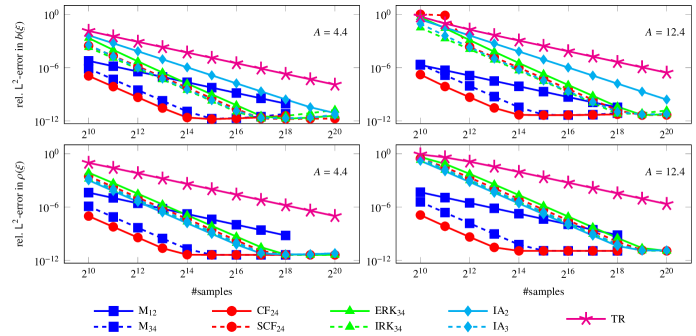
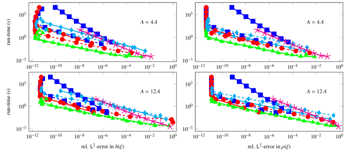
Figure 1: The figure shows the convergence analysis of various methods for the secant-hyperbolic profile. It is evident that the CF method with two exponentials (CF₂₄) outperforms fourth order Magnus method (M₃₄). Note that the complexity of methods M₁₂, M₃₄ and CF₂₄ is $O(N^{2})$ while the rest are of $O(N\log^{2}N)$.

Figure 2: The figure shows the accuracy-complexity trade-off for various methods for the secant-hyperbolic profile. The legends are same as that of Fig. 2. The plots demonstrate that the Runge-Kutta methods (ERK₃₄, IRK₃₄) turn out to be far superior than all the other ‘fast’ methods with regard to the accuracy-complexity trade-off. It is interesting to note that the ‘slow’ methods become quite competitive with increasing signal strength.

For moderately small step-sizes, most fast methods yield poor accuracy specially corresponding to the large values of the spectral parameter. An error analysis of such integrating factor based methods [5] shows that the error terms contain positive powers of the spectral parameter which necessitates the use of smaller step-sizes in order to keep the error low. On the contrary, integrators based on Magnus series expansion are known to have error terms that contain negative powers of the spectral parameter. In this letter, we follow the recipe presented by Blanes et al. [7] to develop a fourth order Magnus method and a fourth order commutator-free (CF) Magnus method [8], both of which take samples of the potential on an equispaced grid in order to compute the NFT. Let us emphasize that our CF method is different from those considered in [9] where the samples of the potential are needed on the Gauss-Legendre nodes (the authors generate the samples by interpolation on an equispaced grid, locally). The fourth-order (standard) Magnus method happens to be faster than the corresponding CF method on account of the fact that there is an additional matrix exponential introduced in the CF method in order to avoid the use of commutators. The accuracy-complexity trade-off, however, is similar for the two methods. Finally, we also present a fast variant of the CF method of order four (formally) by employing the fourth order splitting on the lines of [10, 6]. Despite the well-known limitation imposed on the order and stability of such techniques as demonstrated by Sheng [11], we do not find any reduction of order within the double precision arithmetic. It is noteworthy that the authors in [6] found the aforementioned splitting worsen in accuracy after a certain step-size. It is also not clear from their analysis if this scheme is convergent in their setting.

We begin our discussion with a brief review of the scattering theory closely following the formalism presented in [12]. The nonlinear Fourier transform of any signal is defined via the Zakharov-Shabat (ZS) scattering problem which can be stated as follows: For $\zeta\in\mathbb{R}$ and $\mathbf{v}=(v_{1},v_{2})^{\intercal}$,

$$\mathbf{v}_{t}=\left[-i\zeta\sigma_{3}+U(t)\right]\mathbf{v}\equiv\mathcal{T}(t;\zeta)\mathbf{v},$$ (1)

where $\sigma_{3}=\operatorname{diag}(1,-1)$. The potential $U(t)$ is defined by $U_{11}=U_{22}=0,\,U_{12}=q(t)$ and $U_{21}=r(t)$ with $r=\kappa q^{*}$ ($\kappa\in\{+1,-1\}$). Here, $\zeta\in\mathbb{R}$ is known as the spectral parameter and $q(t)$ is the complex-valued signal. The solution of the scattering problem (1), henceforth referred to as the ZS problem, consists in finding the so called scattering coefficients which are defined through special solutions of (1) known as the Jost solutions which are linearly independent solutions of (1) such that they have a plane-wave like behavior at $+\infty$ or $-\infty$. The Jost solution of the second kind, denoted by $\bm{\phi}(t,\zeta)$, has the asymptotic behavior $\bm{\phi}(t;\zeta)e^{i\zeta t}\rightarrow(1,0)^{\intercal}$ as $t\rightarrow-\infty$. The asymptotic behavior $\bm{\phi}(t;\zeta)\rightarrow(a(\zeta)e^{-i\zeta t},b(\zeta)e^{i\zeta t})^{\intercal}$ as $t\rightarrow\infty$ determines the scattering coefficients $a(\zeta)$ and $b(\zeta)$ for $\zeta\in\mathbb{R}$. In this letter, we primarily focus on the continuous spectrum, also referred to as the reflection coefficient, which is defined by $\rho(\xi)={b(\xi)}/{a(\xi)}$ for $\xi\in\mathbb{R}$.

II The Numerical Scheme

II-A Runge-Kutta Method

In this section, we will develop the integrating factor based exponential Runge-Kutta (RK) method for the numerical solution of the ZS problem. Following [1, 3], we begin with the transformation $\tilde{\mathbf{v}}=e^{i\sigma_{3}\zeta t}\mathbf{v}$ so that (1) becomes $\tilde{\mathbf{v}}_{t}=\widetilde{U}\tilde{\mathbf{v}}$ with $\widetilde{U}=e^{i\sigma_{3}\zeta t}Ue^{-i\sigma_{3}\zeta t}$ whose entries are $\widetilde{U}_{11}=\widetilde{U}_{22}=0,\,\widetilde{U}_{12}=q(t)e^{2i\zeta t}$ and $\widetilde{U}_{21}=r(t)e^{-2i\zeta t}$. Let the step size be $h>0$ and the quantities $c_{j}\in[0,1]$ be ordered so that the nodes within the step can be stated as $t_{n}\leq t_{n}+c_{1}h\leq t_{n}+c_{2}h\leq\ldots\leq t_{n}+c_{s}h\leq t_{n+1}$. For the potential sampled at these nodes, we use the convention $Q_{n+c_{k}}=hq(t_{n}+c_{k}h)$, $R_{n+c_{k}}=hr(t_{n}+c_{k}h)$ and $\widetilde{U}_{n+c_{k}}=\widetilde{U}(t_{n}+c_{k}h)$. In order for the resulting discrete system to be amenable to FFT-based fast polynomial arithmetic, it is sufficient to have each of the $c_{i}$’s belong to the set of uniformly distributed nodes in $[0,1]$. A $s$-stage RK method is characterized by the nodes $\mathbf{c}=(c_{1},c_{2},\ldots,c_{s})\in\mathbb{R}^{s}$, and, the weights $\mathbf{b}=(b_{1},b_{2},\ldots,b_{s})\in\mathbb{R}^{s}$ and $(a_{ij})\in\mathbb{R}^{s\times s}$. Introducing the intermediate stage quantities $\tilde{\mathbf{v}}_{n,k}$ for $k=1,2,\ldots,s$, we have

$$\left\{\begin{aligned} &\tilde{\mathbf{v}}_{n,j}=\tilde{\mathbf{v}}_{n}+h\sum_{k=1}^{s}a_{jk}\widetilde{U}_{n+c_{k}}\tilde{\mathbf{v}}_{n,k},\quad j=1,2,\ldots,s,\\ &\tilde{\mathbf{v}}_{n+1}=\tilde{\mathbf{v}}_{n}+h\sum_{k=1}^{s}b_{k}\widetilde{U}_{n+c_{k}}\tilde{\mathbf{v}}_{n,k}.\end{aligned}\right.$$ (2)

This system of equations can be solved in any computer algebra system to obtained the transfer matrix connecting the vectors $\mathbf{v}_{n+1}$ to $\mathbf{v}_{n}$.

Setting $z=\exp(i\zeta h/2)$, the Lobatto IIIA method (labelled as IRK₃₄) of order $4$ [13] simplifies to

$${\mathbf{v}}_{n+1} ={z^{-2}}\left[\Delta_{n+1}(z^{2})\right]^{-1}M_{n+1}(z^{2}){\mathbf{v}}_{n},$$ (3)

$$M_{n+1} =\begin{pmatrix}1+\frac{z^{2}}{12}Q_{n+1}R_{n+1/2}&\frac{z^{2}}{6}Q_{n+1}+\frac{1}{3}Q_{n+1/2}\\ \frac{1}{6}R_{n+1}+\frac{z^{2}}{3}R_{n+1/2}&z^{2}+\frac{1}{12}R_{n+1}Q_{n+1/2}\end{pmatrix}$$

$$\quad\times\begin{pmatrix}1+\frac{z^{2}}{12}R_{n}Q_{n+1/2}&\frac{1}{6}Q_{n}+\frac{z^{2}}{3}Q_{n+1/2}\\ \frac{z^{2}}{6}R_{n}+\frac{1}{3}R_{n+1/2}&z^{2}+\frac{1}{12}Q_{n}R_{n+1/2}\end{pmatrix},$$ (4)

$$\Delta_{n+1} =\left(1+\frac{z^{-2}}{12}R_{n+1}Q_{n+1/2}\right)\left(1+\frac{z^{2}}{12}Q_{n+1}R_{n+1/2}\right)$$

$$\quad-\frac{1}{36}\left(Q_{n+1}+2{z^{-2}}Q_{n+1/2}\right)\left(R_{n+1}+2{z^{2}}R_{n+1/2}\right).$$ (5)

The fourth order classical RK method (labelled as ERK₃₄) simplifies to the form (3) with $\Delta_{n+1}=1$ and the entries of the transfer matrix are given by

$$\left\{\begin{aligned} M^{(n+1)}_{11}(z^{2})&=G_{n+1/2}+\frac{z^{2}}{6}\left(Q_{n+1/2}R_{n}+Q_{n+1}R_{n+1/2}\right)\\ &\quad+\frac{z^{4}}{24}Q_{n+1/2}Q_{n+1}R_{n}R_{n+1/2},\\ M^{(n+1)}_{22}(z^{2})&=\frac{1}{24}Q_{n}Q_{n+1/2}R_{n+1/2}R_{n+1}+G_{n+1/2}z^{4}\\ &\quad+\frac{z^{2}}{6}\left(Q_{n}R_{n+1/2}+Q_{n+1/2}R_{n+1}\right),\\ M^{(n+1)}_{12}(z^{2})&=\left(\frac{z^{2}}{6}Q_{n}+\frac{z^{4}}{6}Q_{n+1}\right)H_{n+1/2}+\frac{2}{3}Q_{n+1/2},\\ M^{(n+1)}_{21}(z^{2})&=\left(\frac{z^{4}}{6}R_{n}+\frac{1}{6}R_{n+1}\right)H_{n+1/2}+\frac{2z^{2}}{3}R_{n+1/2},\end{aligned}\right.$$ (6)

where $6G_{n+1/2}-6=Q_{n+1/2}R_{n+1/2}=2H_{n+1/2}-2$.

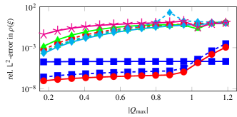
Figure 3: The figure shows the error behavior of the NFT algorithms for $N=2^{10}$ as a function of $Q_{\text{max}}=h\|q\|_{\infty}$ for the secant-hyperbolic profile. The legends are same as that of Fig. 2. It is straightforward to conclude that for smaller number of samples, the ‘slower’ methods (M₁₂, M₃₄ and CF₂₄) are far superior to the ‘fast’ methods for $\xi\in\Omega_{h}$, the principal domain of a given method, with comparable run-times.

II-A1 Scattering coefficients

Let the computational domain be $\Omega=[T_{1},T_{2}]$ and set $2T=T_{2}-T_{1}$. Let the number of steps be $N_{s}$ and $h=2T/N_{s}$. Also, let $h\ell_{+}=T_{2}$ and $h\ell_{-}=-T_{1}$. The grid is defined by $t_{n}=T_{1}+nh/2,\,\,n=0,1,\ldots,N,$ with $t_{N}=T_{2}$ where $N=2N_{s}$ is the number of samples. Let the potential $q(t)$ be supported in $\Omega$ and we assume $q_{0}=0$ for convenience. In order to represent the Jost solutions, we introduce the polynomial vector

$$\mathbf{P}_{n}(z)=\begin{pmatrix}P^{(n)}_{1}(z)\\ P^{(n)}_{2}(z)\end{pmatrix}=\sum_{j=0}^{2n}\mathbf{P}^{(n)}_{j}z^{j}=\sum_{j=0}^{2n}\begin{pmatrix}P^{(n)}_{1,j}\\ P^{(n)}_{2,j}\end{pmatrix}z^{j},$$ (7)

and the polynomial $D_{n}(z)=\sum_{j=0}^{2n}D^{(n)}_{j}z^{j}$. Consider the Jost solution $\phi(t;\zeta)$. For the Lobatto IIIA method, the Jost solution can be stated as $\bm{\phi}_{n}(z^{2})=(z^{2})^{\ell_{-}}\left[D_{n}(z^{2})\right]^{-1}{\mathbf{P}_{n}(z^{2})}$, with

$$\mathbf{P}_{n+1}(z^{2})=\Theta^{-1}_{n+1}M_{n+1}(z^{2})\mathbf{P}_{n}(z^{2}),$$ (8)

where $\Theta_{n}$ is the constant part of $\Delta_{n}(z^{2})$ and

$$D_{n+1}(z^{2})=\Theta^{-1}_{n+1}z^{2}\Delta_{n+1}(z^{2})D_{n}(z^{2}).$$ (9)

From ${\bm{\phi}}(T_{2};\zeta)=\left(ae^{-i\zeta T_{2}},be^{+i\zeta T_{2}}\right)^{\intercal}$, it follows that the discrete scattering coefficients are given by

$$\begin{split}&a_{N_{s}}(z^{2})=(z^{2})^{\ell_{-}+\ell_{+}}{D^{-1}_{N_{s}}(z^{2})}{P^{(N_{s})}_{1}(z^{2})},\\ &b_{N_{s}}(z^{2})=(z^{2})^{\ell_{-}-\ell_{+}}{D^{-1}_{N_{s}}(z^{2})}{P_{2}^{(N_{s})}(z^{2})},\end{split}$$ (10)

where $z=\exp(i\zeta h/2)$. For the classical fourth order RK method, $\Delta_{n}(z^{2})=\Theta_{n}=1$; therefore, $a_{N_{s}}(z^{2})={P^{(N_{s})}_{1}(z^{2})}$ and $b_{N_{s}}(z^{2})=(z^{2})^{-2\ell_{+}}{P_{2}^{(N_{s})}(z^{2})}$. The principal branch for the discrete scattering coefficients here works out to be $\operatorname{Re}\zeta\in[-\pi/2h,\pi/2h]$. This follows from the principle branch of the individual transfer matrices. The nodes $\zeta_{j}=\xi_{j}+i0=j(\pi/h)/N,\,j\in\mathbb{Z},$ lead to $z_{j}^{2}=\exp(i\pi j/N)$ which is not in the standard form for FFT algorithms to be used. Therefore, we would like to work with $N^{\prime}=2N$ nodes so that $z_{j}^{2}=\exp(i2\pi j/N^{\prime})$ and pad the input vector with zeros. Following as in [3], the complexity of computing the scattering coefficient works out to be $O(N\log^{2}N)$.

II-B Standard and commutator-free Magnus methods

II-B1 Magnus method

Let us assume that the solution of the ODE (1) can be written as $\mathbf{v}(t)=\exp[\Lambda(t;t_{n})]\mathbf{v}(t_{n})$ for $t\in[t_{n+1},t_{n}]$, then $\Lambda(t;t_{n})$ has a series representation known as the Magnus series [7]. Truncating this series to achieve the desired order of accuracy yields a family of numerical schemes known as Magnus method. For the ZS problem, Magnus integrators preserve the Lie group structure of the Jost solution and its accuracy does not worsen with increasing $|\zeta|$. In designing a fourth order Magnus integrator (labelled as M₃₄), we follow the method due to Blanes et al. [7, 8]: Defining

$$\mathcal{T}_{n+1}^{(j)}(h;\zeta)=h\int_{0}^{1}\left(\tau-\frac{1}{2}\right)^{j}\mathcal{T}(t_{n}+\tau h;\zeta)d\tau,$$ (11)

the method proceeds by expanding $\Lambda(t_{n+1};t_{n})$ in terms of the quantities $\mathcal{T}_{n+1}^{(j)}(h;\zeta)$ using the Magnus series. For the fourth order method, setting $\Lambda(t_{n+1};t_{n})\approx\Lambda_{n+1}$, we have [7, 8] $\Lambda_{n+1}=\mathcal{T}_{n+1}^{(0)}+\left[\mathcal{T}_{n+1}^{(1)},\mathcal{T}_{n+1}^{(0)}\right]$. Evaluating $\mathcal{T}_{n+1}^{(0)}$ and $\mathcal{T}_{n+1}^{(1)}$ upto fourth order accuracy using the three-point Gauss quadrature involving Legendre-Gauss-Lobatto (LGL) nodes, $\mathbf{c}=(0,{1}/{2},1)$, the numerical scheme for the ZS problem can be stated as $\mathbf{v}_{n+1}=\exp(\Lambda_{n+1})\mathbf{v}_{n}$ where,

$$\Lambda_{n+1}=\begin{pmatrix}\Xi_{n+1}&G_{n+1}\\ H_{n+1}&-\Xi_{n+1}\end{pmatrix}+i\zeta h\begin{pmatrix}-1&\frac{(Q_{n+1}-Q_{n})}{6}\\ \frac{(R_{n}-R_{n+1})}{6}&1\end{pmatrix},$$ (12)

where $6G_{n+1}=(Q_{n}+4Q_{n+1/2}+Q_{n+1})$, $H_{n+1}=\kappa G^{*}_{n+1}$ and $12\Xi_{n+1}=[(Q_{n+1}-Q_{n})H_{n+1}-(R_{n+1}-R_{n})G_{n+1}]$. For the purpose of comparison, we would also like to consider the Magnus method with one point Gauss quadrature (labelled as M₁₂) which is of order $2$ [1].

II-B2 Commutator-free Magnus method

Blanes and Moan [8] have constructed fourth-order commutator-free (CF) methods that are based on Magnus method. Using the quantities defined above, the CF method (labelled as CF₂₄) can be stated as

$$\mathbf{v}_{n+1}=e^{\Lambda^{(+)}_{n+1}}e^{\Lambda^{(-)}_{n+1}}\mathbf{v}_{n},\quad 2\Lambda^{(\pm)}_{n+1}=\mathcal{T}_{n+1}^{(0)}\pm 4\mathcal{T}_{n+1}^{(1)}.$$ (13)

Evaluating $\mathcal{T}^{(0)}_{n+1}$ and $\mathcal{T}^{(1)}_{n+1}$ upto fourth-order accuracy using the three-point Gauss quadrature involving LGL nodes, we have $2\Lambda^{(\pm)}_{n+1}=-{i\zeta h\sigma_{3}}+2h\mathcal{U}^{(\pm)}_{n+1}$ where $[\mathcal{U}^{(\pm)}_{n+1}]_{11}=[\mathcal{U}^{(\pm)}_{n+1}]_{22}=0$,

$$\begin{split}&h[\mathcal{U}^{(+)}_{n+1}]_{12}\equiv G^{(+)}_{n+1}=(3Q_{n+1}+4Q_{n+1/2}-Q_{n})/12,\\ &h[\mathcal{U}^{(-)}_{n+1}]_{12}\equiv G^{(-)}_{n+1}=(3Q_{n}+4Q_{n+1/2}-Q_{n+1})/12,\\ \end{split}$$ (14)

and $h[\mathcal{U}^{(\pm)}_{n+1}]_{21}\equiv H^{(\pm)}_{n+1}=\kappa h[\mathcal{U}^{(\pm)}_{n+1}]^{*}_{12}$. Given that there are two matrix exponentials involved, the CF Magnus method has higher complexity than that of the standard Magnus method.

II-B3 A fast variant

The CF Magnus method further allows us to obtain a fast NFT algorithm (labelled as SCF₂₄) via splitting of the matrix exponential. Consider a formally fourth order splitting [10]:

$$3e^{\Lambda^{(\pm)}_{n+1}}=4\left(e^{-\frac{1}{8}i\zeta h\sigma_{3}}e^{\frac{1}{2}h\mathcal{U}^{(\pm)}_{n+1}}e^{-\frac{1}{8}i\zeta h\sigma_{3}}\right)^{2}\\ -e^{-\frac{1}{4}i\zeta h\sigma_{3}}e^{h\mathcal{U}^{(\pm)}_{n+1}}e^{-\frac{1}{4}i\zeta h\sigma_{3}}+\mathop{\mathcal{O}}\left(h^{5}\right).$$ (15)

This splitting is stable and convergent [10]; however, its global order of convergence is $\leq 2$ [11]. Introducing $16\Delta^{(\pm)}_{n+1}=12-3G_{n+1}^{(\pm)}H_{n+1}^{(\pm)}$ and $\Theta^{(\pm)}_{n+1}=1-G^{(\pm)}_{n+1}H^{(\pm)}_{n+1}$, and, putting $z=\exp(i\zeta h/4)$, the transfer matrix relation can be written as

$$\mathbf{v}_{n+1}={z^{-4}}\left[\Delta^{(+)}_{n+1}\Delta^{(-)}_{n+1}\right]^{-1}M^{(+)}_{n+1}(z)M^{(-)}_{n+1}(z)\mathbf{v}_{n},$$ (16)

where the entries of the matrix $M^{(\pm)}_{n+1}(z)$ are

$$\left\{\begin{aligned} &M^{(\pm,n+1)}_{11}(z)=\left(1-C^{(\pm)}_{n+1}\right)+\frac{z^{2}}{4}G_{n+1}^{(\pm)}H_{n+1}^{(\pm)},\\ &M^{(\pm,n+1)}_{22}(z)=\left(1-C^{(\pm)}_{n+1}\right)z^{4}+\frac{z^{2}}{4}G_{n+1}^{(\pm)}H_{n+1}^{(\pm)},\\ &M^{(\pm,n+1)}_{12}(z)=\frac{z}{2}\left(1+z^{2}\right)G_{n+1}^{(\pm)}-z^{2}C^{(\pm)}_{n+1}G_{n+1}^{(\pm)},\\ &M^{(\pm,n+1)}_{21}(z)=\frac{z}{2}\left(1+z^{2}\right)H_{n+1}^{(\pm)}-z^{2}C^{(\pm)}_{n+1}H_{n+1}^{(\pm)},\end{aligned}\right.$$ (17)

where $3C^{(\pm)}_{n+1}={\Delta^{(\pm)}_{n+1}}[\Theta^{(\pm)}_{n+1}]^{-1/2}$. The discrete scattering coefficients can be written as $a_{N_{s}}(z)={P^{(2N_{s})}_{1}(z)}$ and $b_{N_{s}}(z)=z^{-8\ell_{+}}{P_{2}^{(2N_{s})}(z)}$. The principal branch for the discrete scattering coefficients here works out to be $\operatorname{Re}\zeta\in[-\pi/2h,\pi/2h]$. This again follows from the principle branch of the individual transfer matrices. As before, the nodes $\zeta_{j}=\xi_{j}+i0=j(\pi/h)/N,\,j\in\mathbb{Z},$ lead to $z_{j}=\exp(i\pi j/4N)$ which is not in the standard form for FFT algorithms to be used. Therefore, we would like to work with $N^{\prime}=8N$ nodes so that $z_{j}=\exp(i2\pi j/N^{\prime})$ and pad the input vector with zeros.

III Numerical Tests and Conclusion

For the numerical experiments, we employ the well-known secant-hyperbolic potential given by $q(t)=A\operatorname{sech}{t}$, ($\kappa=-1$) for which the scattering coefficients are given in [1]. We set the computational domain to be $[-30,30]$ and let $A\in\{4.4,12.4\}$. Let $\Omega_{h}$ be the principal branch; then, the error in computing $b(\xi)$ is quantified by

$$e_{\text{rel.}}=\|b(\xi)-b_{N}(\xi)\|_{\mathsf{L}^{2}(\Omega_{h})}/\|b(\xi)\|_{\mathsf{L}^{2}(\Omega_{h})},$$ (18)

where the integrals are computed using the trapezoidal rule. Similar consideration applies to $\rho(\xi)$. For the purpose of testing, we include the implicit Adams method presented in [3] which are labelled as IA_m with $m=2,3$. The method IA₁ is identical to the trapezoidal rule, therefore, we use the label TR. The convergence analysis is carried out in Fig. 2 and the trade-off between accuracy and complexity is presented in Fig. 2. In terms of accuracy, the CF₂₄ outperforms every other method with M₃₄ being a close second. However, the accuracy-complexity trade-off is similar for the two methods. The ‘fast’ methods evidently lower complexity at the cost of accuracy. The RK methods (ERK₃₄ and IRK₃₄) outperform all the other ’fast’ methods in terms of accuracy-complexity trade-off (see Fig. 2); however, with increasing signal strength, the ‘slow’ methods becoming equally competitive. In fact, at moderately small step-sizes, the ‘slow’ methods far outperform the ‘fast’ methods (see Fig. 3) with increasing signal strength.

References

• [1] V. Vaibhav, “Fast inverse nonlinear Fourier transformation using exponential one-step methods: Darboux transformation,” Phys. Rev. E, vol. 96, p. 063302, 2017.
• [2] ——, “Fast inverse nonlinear Fourier transform,” Phys. Rev. E, vol. 98, p. 013304, 2018.
• [3] ——, “Higher order convergent fast nonlinear Fourier transform,” IEEE Photonics Technol. Lett., vol. 30, no. 8, pp. 700–703, 2018.
• [4] S. Wahls and H. V. Poor, “Fast numerical nonlinear Fourier transforms,” IEEE Trans. Inf. Theory, vol. 61, no. 12, pp. 6957–6974, 2015.
• [5] S. Burtsev, R. Camassa, and I. Timofeyev, “Numerical algorithms for the direct spectral transform with applications to nonlinear Schrödinger type systems,” J. Comput. Phys., vol. 147, no. 1, pp. 166–186, 1998.
• [6] S. Chimmalgi, P. J. Prins, and S. Wahls, “Fast nonlinear Fourier transform algorithms using higher order exponential integrators,” 2018, arXiv:1812.00703[eess.SP]. [Online]. Available: https://arxiv.org/abs/1812.00703
• [7] S. Blanes, F. Casas, and J. Ros, “Improved high order integrators based on the magnus expansion,” BIT Numer. Math., vol. 40, no. 3, pp. 434–450, 2000.
• [8] S. Blanes and P. C. Moan, “Fourth- and sixth-order commutator-free Magnus integrators for linear and non-linear dynamical systems,” Appl. Numer. Math., vol. 56, no. 12, pp. 1519–1537, 2006.
• [9] S. Chimmalgi, P. J. Prins, and S. Wahls, “Nonlinear Fourier transform algorithm using a higher order exponential integrator,” in Signal Processing in Photonic Communications, 2018, p. SpM4G.5.
• [10] S. Descombes, “Convergence of a splitting method of high order for reaction-diffusion systems,” Mathematics of Computation, vol. 70, no. 236, pp. 1481–1501, 2001. [Online]. Available: http://www.jstor.org/stable/2698737
• [11] Q. Sheng, “Solving linear partial differential equations by exponential splitting,” IMA J. Numer. Anal., vol. 9, no. 2, pp. 199–212, 1989.
• [12] M. J. Ablowitz, D. J. Kaup, A. C. Newell, and H. Segur, “The inverse scattering transform - Fourier analysis for nonlinear problems,” Stud. Appl. Math., vol. 53, no. 4, pp. 249–315, 1974.
• [13] J. C. Butcher, Numerical Methods for Ordinary Differential Equations, 2nd ed.   San Francisco: John Wiley & Sons, Ltd, 2003.