Explicit time-discretisation of elastodynamics with some inelastic processes at small strains.


Tomáš Roubíček111Charles University, Mathematical Institute, Sokolovská 83, CZ-186 75 Praha 8, Czech Republic, tomas.roubicek@mff.cuni.cz,222Institute of Thermomechanics of the Czech Acad. Sci., Dolejškova 5, CZ–182 08 Praha 8, Czech Rep., Christos G. Panagiotopoulos333Institute of Applied and Computational Mathematics, Foundation for Research and Technology - Hellas, Nikolaou Plastira 100, Vassilika Vouton, GR-700 13 Heraklion, Crete, Greece pchr@iacm.forth.gr, Chrysoula Tsogka444Applied Math Unit, UC Merced, 5200 North Lake Road, Merced, CA 95343, USA, ctsogka@ucmerced.edu,33footnotemark: 3


Abstract: The 2-step staggered (also called leap-frog) time discretisation of linear 2nd-order Hamiltonian systems (typically linear elastodynamics in a stress-velocity form) is extended for a 3-step staggered discretisation applicable for systems involving some internal variables subjected to a dissipative evolution. After spatial discretisation, a-priori estimates and convergence is proved under the usual CFL-condition. Applications to specific problems in continuum mechanics of solids at small stains are considered, in particular linearized plasticity, diffusion in poroelastic media, damage, or adhesive contact. Numerical implementation and some computational 2-dimensional simulation of waves emitted by a rupture (delamination) of an adhesive contact illustrate the abstract theory and efficiency of the explicit method.

Keywords: elastodynamics, explicit staggered discretisation, mixed finite-element method, plasticity, poroelasticity, damage, adhesive contact.

AMS Classification: 65M12, 65P10, 65Z05, 74C10, 74F10, 74H15, 74M15, 74R20, 74S05, 76S05.

1 Introduction – mere linear elastodynamics

In computational continuum mechanics of elastic or viscoelastic solids, so-called transient (low-frequency) and wave propagation problems(high-frequency) are distinguished and different approximation methods are used. The prototype equation or rather initial-boundary-value problem which we have in mind is the linear elastodynamic at small strains:

$\displaystyle\varrho\mathchoice{{\buildrel\hskip 1.00006pt\text{\LARGE..}\over{u}}}{{\buildrel\hskip 1.00006pt\text{\Large..}\over{u}}}{{\buildrel\hskip 1.00006pt\text{\large..}\over{u}}}{{\buildrel\hskip 1.00006pt\text{\large..}\over{u}}}-{\rm div}\,\mathbb{C}e(u)=f$ $\displaystyle\text{on }\ \varOmega\ \text{ for }\ t\in[0,T],$ (1.1a)
$\displaystyle[\mathbb{C}e(u)]\vec{n}+\mathbb{B}u=g$ $\displaystyle\text{on }\ \varGamma\ \text{ for }\ t\in[0,T],$ (1.1b)
$\displaystyle u|_{t=0}=u_{0},\ \ \ \mathchoice{{\buildrel\hskip 1.00006pt\text{\LARGE.}\over{u}}}{{\buildrel\hskip 1.00006pt\text{\Large.}\over{u}}}{{\buildrel\hskip 1.00006pt\text{\large.}\over{u}}}{{\buildrel\hskip 1.00006pt\text{\large.}\over{u}}}|_{t=0}=v_{0}$ $\displaystyle\text{on }\ \varOmega,$ (1.1c)

with $\varrho>0$ a mass density, $\mathbb{C}$ a symmetric positive definite 4th-order elasticity tensor, $e(u)=\frac{1}{2}(\nabla u)^{\top}{+}\frac{1}{2}\nabla u$ the small-strain tensor, $\mathbb{B}$ a symmetric positive semidefinite 2nd-order tensor determining the elastic support on the boundary, $f$ the bulk force, $g$ the surface loading, $u_{0}$ the prescribed initial displacement, $v_{0}$ initial velocity, and $T>0$ a fixed time horizon. The unknown $u:[0,T]\varOmega\to{\mathbb{R}}^{d}$ is the displacement, the dot-notation stands for the time derivative, $\Omega\subset{\mathbb{R}}^{d}$ is a bounded Lipschitz domain, $d=2$ or $3$, $\varGamma$ is its boundary, and $\vec{n}$ the unit outward normal. For notational simplicity, we will write the initial-boundary-value problem (1.1) in the abstract form

$\displaystyle\mathcal{T}^{\prime}\mathchoice{{\buildrel\hskip 1.00006pt\text{\LARGE..}\over{u}}}{{\buildrel\hskip 1.00006pt\text{\Large..}\over{u}}}{{\buildrel\hskip 1.00006pt\text{\large..}\over{u}}}{{\buildrel\hskip 1.00006pt\text{\large..}\over{u}}}+\mathcal{W}^{\prime}u=\mathcal{F}_{u}^{\prime}(t)\ \ \text{ for }\ t\in[0,T],\ \ u|_{t=0}=u_{0},\ \ \ \mathchoice{{\buildrel\hskip 1.00006pt\text{\LARGE.}\over{u}}}{{\buildrel\hskip 1.00006pt\text{\Large.}\over{u}}}{{\buildrel\hskip 1.00006pt\text{\large.}\over{u}}}{{\buildrel\hskip 1.00006pt\text{\large.}\over{u}}}|_{t=0}=v_{0},$ (1.2)

where $\mathcal{T}$ is the kinetic energy, $\mathcal{W}$ is the stored energy, and $\mathcal{F}$ is the external force, while $(\cdot)^{\prime}$ denotes the Gâteaux derivative. In the context of (1.1), $\mathcal{T}(v)=\int_{\varOmega}\frac{1}{2}\varrho|v|^{2}\,\mathrm{d}x$, $\mathcal{W}(u)=\int_{\varOmega}\frac{1}{2}\mathbb{C}e(u){:}e(u)\,\mathrm{d}x+\int_{\varGamma}\frac{1}{2}\mathbb{B}u\cdot u\,\mathrm{d}S$, and $\mathcal{F}(t,u)=\int_{\varOmega}f(t){\cdot}u\,\mathrm{d}x+\int_{\varGamma}g(t){\cdot}u\,\mathrm{d}S$. Thus $\mathcal{F}_{u}^{\prime}(t)$ is the linear functional, let us denote it shortly by $F(t)$.

In situations where high-frequency oscillations arising typically during wave propagation are to be calculated, the implicit time-discretisations (even if energy conserving as e.g. [32, 38]) are computationally cumbersome especially in 3-dimensional problems. Hence explicit time discretisations are more efficient. The simplest explicit scheme is the so-called central-difference scheme

$\displaystyle\mathcal{T}^{\prime}\frac{u_{\tau h}^{k+1}-2u_{\tau h}^{k}+u_{\tau h}^{k-1}}{\tau^{2}}+\mathcal{W}_{h}^{\prime}u_{\tau h}^{k}=F_{h}(k\tau)$ (1.3)

with $\tau>0$ a time step, and with $\mathcal{W}_{h}$ and $F_{h}$ denoting some approximations of the respective functionals obtained by a suitable finite-element method (FEM) with the mesh size $h>0$. In particular, a numerical approximation leading to a diagonalization of the mass matrix $\mathcal{T}^{\prime}$, called mass lumping, in (1.3) is an important ingredient so as to obtain efficient explicit methods. The formula (1.3) leads, when tested by $\frac{u_{\tau h}^{k+1}-u_{\tau h}^{k}}{\tau}$, to a correct discrete kinetic energy $\mathcal{T}$ but a twisted stored energy, namely $\frac{1}{2}\langle\mathcal{W}_{h}^{\prime}u_{\tau h}^{k+1},u_{\tau h}^{k}\rangle$, whose handling needs the Courant-Fridrichs-Lewy (CFL) condition [15] that typically bounds the time discretisation step $\tau=\mathscr{O}(h_{\rm min})$ with $h_{\rm min}$ the smallest element size on a FEM discretisation cf. [45, p.171] or also e.g. [25, 30]. More specifically, the CFL reads as

$\displaystyle\big{\langle}\mathcal{T}^{\prime}u_{h},u_{h}\big{\rangle}\geq\frac{\tau^{2}}{4}\big{\langle}{\cal W}_{h}^{\prime}u_{h},u_{h}\big{\rangle}$ (1.4)

for any $u_{h}$ from the respective finite-dimensional subspace. This is a drawback which makes such discretisation less suitable for enhancing the stored energy by some internal variables and (possibly) nonlinear processes on them, which is the goal of this article.

Therefore, we use another, so-called leap-frog, scheme. To this aim, we first rewrite (1.1a) in in the velocity/stress formulation, i.e. terms of $v=\mathchoice{{\buildrel\hskip 1.00006pt\text{\LARGE.}\over{u}}}{{\buildrel\hskip 1.00006pt\text{\Large.}\over{u}}}{{\buildrel\hskip 1.00006pt\text{\large.}\over{u}}}{{\buildrel\hskip 1.00006pt\text{\large.}\over{u}}}$ and of the stress $\sigma:=\mathbb{C}e(u)$, eliminating the displacement $u$, further we consider the rate form of (1.1b), together with appropriate initial conditions:

$\displaystyle\varrho\mathchoice{{\buildrel\hskip 1.00006pt\text{\LARGE.}\over{v}}}{{\buildrel\hskip 1.00006pt\text{\Large.}\over{v}}}{{\buildrel\hskip 1.00006pt\text{\large.}\over{v}}}{{\buildrel\hskip 1.00006pt\text{\large.}\over{v}}}-{\rm div}\,\sigma=f\ \ \ \text{ and }\ \ \ \mathchoice{{\buildrel\hskip 1.00006pt\text{\LARGE.}\over{\sigma}}}{{\buildrel\hskip 1.00006pt\text{\Large.}\over{\sigma}}}{{\buildrel\hskip 1.00006pt\text{\large.}\over{\sigma}}}{{\buildrel\hskip 1.00006pt\text{\large.}\over{\sigma}}}=\mathbb{C}e(v)$ $\displaystyle\text{on }\ \varOmega\ \text{ for }\ t\in[0,T],$ (1.5a)
$\displaystyle\mathchoice{{\buildrel\hskip 1.00006pt\text{\LARGE.}\over{\sigma}}}{{\buildrel\hskip 1.00006pt\text{\Large.}\over{\sigma}}}{{\buildrel\hskip 1.00006pt\text{\large.}\over{\sigma}}}{{\buildrel\hskip 1.00006pt\text{\large.}\over{\sigma}}}\vec{n}+\mathbb{B}v=\mathchoice{{\buildrel\hskip 1.00006pt\text{\LARGE.}\over{g}}}{{\buildrel\hskip 1.00006pt\text{\Large.}\over{g}}}{{\buildrel\hskip 1.00006pt\text{\large.}\over{g}}}{{\buildrel\hskip 1.00006pt\text{\large.}\over{g}}}$ $\displaystyle\text{on }\ \varGamma\ \text{ for }\ t\in[0,T],$ (1.5b)
$\displaystyle v|_{t=0}=v_{0},\ \ \ \sigma|_{t=0}=\sigma_{0}:=\mathbb{C}e(u_{0})$ $\displaystyle\text{on }\ \varOmega.$ (1.5c)

In the abstract form (1.2), when writing $\mathcal{W}=\mathscr{W}\circ E$ with $E$ denoting the linear operator $u\mapsto(e,w):=(e(u),u|_{\varGamma})$, this reads as

$\displaystyle\mathcal{T}^{\prime}\mathchoice{{\buildrel\hskip 1.00006pt\text{\LARGE.}\over{v}}}{{\buildrel\hskip 1.00006pt\text{\Large.}\over{v}}}{{\buildrel\hskip 1.00006pt\text{\large.}\over{v}}}{{\buildrel\hskip 1.00006pt\text{\large.}\over{v}}}+E^{*}\varSigma=F(t)$ $\displaystyle\text{ for }\ t\in[0,T],$ $\displaystyle v|_{t=0}=v_{0},\ \ \ \ \text{ and }$ (1.6a)
$\displaystyle\mathchoice{{\buildrel\hskip 1.00006pt\text{\LARGE.}\over{\varSigma}}}{{\buildrel\hskip 1.00006pt\text{\Large.}\over{\varSigma}}}{{\buildrel\hskip 1.00006pt\text{\large.}\over{\varSigma}}}{{\buildrel\hskip 1.00006pt\text{\large.}\over{\varSigma}}}=\mathscr{W}^{\prime}Ev+\mathchoice{{\buildrel\hskip 1.00006pt\text{\LARGE.}\over{G}}}{{\buildrel\hskip 1.00006pt\text{\Large.}\over{G}}}{{\buildrel\hskip 1.00006pt\text{\large.}\over{G}}}{{\buildrel\hskip 1.00006pt\text{\large.}\over{G}}}(t)$ $\displaystyle\text{ for }\ t\in[0,T],$ $\displaystyle\varSigma|_{t=0}=\varSigma_{0}:=\mathscr{W}^{\prime}Eu_{0},$ (1.6b)

where $E^{*}$ is the adjoint operator to $E$. The stored energy governing (1.5) is $\mathscr{W}(e,w)=\int_{\varOmega}\frac{1}{2}\mathbb{C}e{:}e\,\mathrm{d}x+\int_{\varGamma}\frac{1}{2}\mathbb{B}w{\cdot}w\,\mathrm{d}S$ while the external loading is now split into two parts acting differently, namely $\langle F(t),u\rangle=\int_{\Omega}f(t)\cdot u\,\mathrm{d}x$ and $\langle G(t),w\rangle=\int_{\varGamma}g(t)\cdot w\,\mathrm{d}x.$ Let us note that (1.6) involves, in fact, the equation on $\varOmega$ as well as the equation on $\varGamma$ if $\mathcal{T}$ understood as the functional on $\varOmega\times\varGamma$, being trivial on $\varGamma$ since no inertial is considered on the $(d{-}1$)-dimensional boundary $\varGamma$. In particular, the “generalized” stress $\varSigma=\mathscr{W}^{\prime}Eu=(\mathbb{C}e(u),\mathbb{B}u|_{\varGamma})$ contains, beside the bulk stress tensor, also the traction stress vector. Relying on the linearity of $\mathscr{W}^{\prime}$, we have $\mathchoice{{\buildrel\hskip 1.00006pt\text{\LARGE.}\over{\varSigma}}}{{\buildrel\hskip 1.00006pt\text{\Large.}\over{\varSigma}}}{{\buildrel\hskip 1.00006pt\text{\large.}\over{\varSigma}}}{{\buildrel\hskip 1.00006pt\text{\large.}\over{\varSigma}}}=\mathscr{W}^{\prime}Ev$ with $v=\mathchoice{{\buildrel\hskip 1.00006pt\text{\LARGE.}\over{u}}}{{\buildrel\hskip 1.00006pt\text{\Large.}\over{u}}}{{\buildrel\hskip 1.00006pt\text{\large.}\over{u}}}{{\buildrel\hskip 1.00006pt\text{\large.}\over{u}}}$, as used in (1.6).

The mentioned “leap-frog” time discretisation of (1.6) then reads as

$\displaystyle\frac{\varSigma_{\tau h}^{k+1/2}-\varSigma_{\tau h}^{k-1/2}}{\tau}=\mathscr{W}^{\prime}E_{h}v_{\tau h}^{k}+D_{\tau h}^{k}\ \ \ \ \ \text{ and }\ \ \ \ {\mathcal{T}}^{\prime}\frac{v_{\tau h}^{k+1}{-}v_{\tau h}^{k}}{\tau}+E_{h}^{*}\varSigma_{\tau h}^{k+1/2}=F_{\tau h}^{k+1/2},$ (1.7)

where $\mathscr{W}_{h}$ and $E_{h}$ is a suitable FEM discretisation of $E$ and

$\displaystyle F_{\tau h}^{k+1/2}:=\frac{1}{\tau}\int_{k\tau}^{(k+1)\tau}\!\!\!\!\!\!\!\!\!\!\!F_{h}(t)\,\mathrm{d}t\ \text{ and }\ \ D_{\tau h}^{k}:=\frac{1}{\tau}\int_{(k-1/2)\tau}^{(k+1/2)\tau}\!\!\mathchoice{{\buildrel\hskip 1.00006pt\text{\LARGE.}\over{G}}}{{\buildrel\hskip 1.00006pt\text{\Large.}\over{G}}}{{\buildrel\hskip 1.00006pt\text{\large.}\over{G}}}{{\buildrel\hskip 1.00006pt\text{\large.}\over{G}}}_{h}(t)\,\mathrm{d}t=\frac{G_{h}((k{+}\frac{1}{2})\tau)-G_{h}((k{-}\frac{1}{2})\tau)}{\tau}.$ (1.8)

We assume that $v$’s is discretised in a piecewise-constant way so that $\mathcal{T}$ leads to a diagonal form on such a subspace and therefore numerical integration leading to mass lumping is not needed here. Otherwise, higher-order discretisation with mass lumping may also be used to achieve the desired property of obtaining an explicit scheme (avoid solving systems of equations). We refer to [7, 22, 45] for details in the case $G\equiv 0$. This discretisation also does not need inversion of $\mathcal{W}_{h}^{\prime}=E_{h}^{*}\mathscr{W}^{\prime}E_{h}$, which is just the ultimate goal of all explicit discretisation schemes. Usually, the spatial FEM discretisation exploits regularity available in linear elastodynamics, in particular that ${\rm div}\,\sigma$ and $e(v)$ in (1.5a) live in $L^{2}$-spaces. Moreover, the equations in (1.7) are decoupled in the sense that, first, $\varSigma_{\tau h}^{k+1/2}$ is calculated from the former equation and, second, $v_{\tau h}^{k+1}$ is calculated from the latter equation assuming, that $(v_{\tau h}^{k},\varSigma_{\tau h}^{k-1/2})$ is known from the previous time step. For $k=0$, it starts from $v_{\tau h}^{0}=v_{0}$ and from a half time step $\varSigma_{\tau h}^{1/2}=\varSigma_{\tau h}^{0}+\frac{\tau}{2}\mathscr{W}^{\prime}E_{h}v_{\tau h}^{0}$. For the space discretisation, the lower order $Q^{\rm div}_{k+1}-Q_{k}$ finite element is obtained for $k=0$ and in this case the velocity is discretised as piecewise constant on rectangular or cubic elements while the stress is discretised by piecewise bi-linear functions with some continuities. Namely the normal component of the stress is continuous across edges of adjacent elements while the tangential component is allowed to be discontinuous. For more details about the space discretisation we refer the interested reader to [7]. An alternative discretisation using triangular elements known as staggered discontinuous Galerkin method is proposed in [13]. In general, the leap-frog scheme has been frequently used in geophysics to calculate seismic wave propagation with the finite differences method, cf. e.g. [9, 18, 46].

When taking the average (i.e. the sum with the weights $\frac{1}{2}$ and $\frac{1}{2}$) of the second equation in (1.7) in the level $k$ and $k{-}1$ tested by $v_{\tau h}^{k}$ and summing it with the first equation in (1.7) tested by $[\mathscr{W}^{\prime}]^{-1}(\varSigma_{\tau h}^{k+1/2}{+}\varSigma_{\tau h}^{k-1/2})/2$, we obtain

$\displaystyle\frac{1}{2\tau}\big{\langle}[\mathscr{W}^{\prime}]^{-1}\varSigma_{\tau h}^{k+1/2},\varSigma_{\tau h}^{k+1/2}\big{\rangle}-\frac{1}{2\tau}\big{\langle}[\mathscr{W}^{\prime}]^{-1}\varSigma_{\tau h}^{k-1/2},\varSigma_{\tau h}^{k-1/2}\big{\rangle}$
$\displaystyle\qquad\qquad=\Big{\langle}\frac{\varSigma_{\tau h}^{k+1/2}{+}\varSigma_{\tau h}^{k-1/2}}{2},E_{h}v_{\tau h}^{k}\Big{\rangle}+\Big{\langle}[\mathscr{W}^{\prime}]^{-1}D_{\tau h}^{k},\frac{\varSigma_{\tau h}^{k+1/2}{+}\varSigma_{\tau h}^{k-1/2}}{2}\Big{\rangle}\ \ \text{ and}$
$\displaystyle\Big{\langle}{\mathcal{T}}^{\prime}\frac{v_{\tau h}^{k+1}{-}v_{\tau h}^{k-1}}{\tau},v_{\tau h}^{k}\Big{\rangle}+\Big{\langle}\frac{\varSigma_{\tau h}^{k+1/2}{+}\varSigma_{\tau h}^{k-1/2}}{2},E_{h}v_{\tau h}^{k}\Big{\rangle}=\Big{\langle}\frac{F_{\tau h}^{k+1/2}{+}F_{\tau h}^{k-1/2}}{2},v_{\tau h}^{k}\Big{\rangle}\,.$

Summing it up, we eventually obtain the (approximate) energy balance with the correct stored energy and twisted discrete kinetic energy, namely

$\displaystyle\frac{1}{2}\langle\mathscr{T}^{\prime}v_{\tau h}^{k+1},v_{\tau h}^{k}\rangle+\varPhi_{h}(\varSigma_{\tau h}^{k+1/2})\ \ \text{ with }\ \ \varPhi_{h}(\varSigma)=\frac{1}{2}\langle[\mathscr{W}^{\prime}]^{-1}\varSigma,\varSigma\rangle\,;$ (1.9)

note that $\varPhi_{h}$ is the (possibly approximate) stored energy but expressed in terms of the generalized stress. Yet, in contrast to (1.3), yielding the energy balance with the correct stored energy, (1.7) allows for enhancement of this stored energy by some internal variables. This last attribute is a qualitative difference compared to (1.3). Again, the a-priori estimates and convergence for $\tau\to 0$ and $h\to 0$ needs the following CFL condition

$\displaystyle\big{\langle}[\mathcal{W}^{\prime}_{h}]^{-1}\varSigma_{h},\varSigma_{h}\big{\rangle}\geq\frac{\tau^{2}}{4}\big{\langle}E^{*}_{h}\varSigma_{h},({\mathcal{T}}^{\prime})^{-1}E^{*}_{h}\varSigma_{h}\big{\rangle}$ (1.10)

for any $\varSigma_{h}$ from the respective finite-dimensional subspace. Moreover, $F=0$ is often considered, which makes the a-priori estimation easier. Let us also note that the adjective “leap-frog” is sometimes used also for the time-discretisation (1.3) if written as a two-step scheme, cf. e.g. [14, Sect. 7.1.1.1].

The plan of this article is as follows: In Section 2, we extend the abstract system (1.6) by another equation for some internal variable and cast its weak formulation without relying on any regularity. Then, in Section 3, we enhance the two-step leap-frog discrete scheme (1.7) to a suitable three-step scheme, and show its energetics. Then, in Section 4, we prove the numerical stability of the 3-step staggered approximation scheme and its convergence under the CFL condition modified correspondingly, cf. (4.1) below. Such an abstract scheme is then illustrated in Section 5 on several examples from continuum mechanics, in particular on models of plasticity, creep, diffusion, damage, and delamination. Eventually, in Section (6), numerical implementation of the presented scheme for problems of adhesive contact is considered and computational experiments are shown in order to demonstrate its computational efficiency.

It should be emphasized that, to the best of our knowledge, a rigorously justified (as far as numerical stability and convergence) combination of the explicit staggered discretisation with nonlinear dissipative processes on some internal variables is new, although occasionally some dissipative nonlinear phenomena can be found in literature as in [40] for a unilateral contact, in [9] for a Maxwell viscoelastic rheology, in [42] for electroactive polymers, or in [16] for general thermomechanical systems, but without any numerical stability (a-priori estimates) and convergence guaranteed.

2 Internal variables and their dissipative evolution.

The concept of internal variables has a long tradition and opens wide options for material modelling while the internal parameters are subjected to 1st-order evolution flow rules, cf. [28]. The system (1.2) is thus enhanced as:

$\displaystyle\mathcal{T}^{\prime}\mathchoice{{\buildrel\hskip 1.00006pt\text{\LARGE..}\over{u}}}{{\buildrel\hskip 1.00006pt\text{\Large..}\over{u}}}{{\buildrel\hskip 1.00006pt\text{\large..}\over{u}}}{{\buildrel\hskip 1.00006pt\text{\large..}\over{u}}}+\mathcal{W}_{u}^{\prime}(u,z)=F(t)$ $\displaystyle\text{ for }\ t\in[0,T],\ \ u|_{t=0}=u_{0},\ \ \ \mathchoice{{\buildrel\hskip 1.00006pt\text{\LARGE.}\over{u}}}{{\buildrel\hskip 1.00006pt\text{\Large.}\over{u}}}{{\buildrel\hskip 1.00006pt\text{\large.}\over{u}}}{{\buildrel\hskip 1.00006pt\text{\large.}\over{u}}}|_{t=0}=v_{0},$ (2.1a)
$\displaystyle\partial\varPsi(\mathchoice{{\buildrel\hskip 1.00006pt\text{\LARGE.}\over{z}}}{{\buildrel\hskip 1.00006pt\text{\Large.}\over{z}}}{{\buildrel\hskip 1.00006pt\text{\large.}\over{z}}}{{\buildrel\hskip 1.00006pt\text{\large.}\over{z}}})+\mathcal{W}_{z}^{\prime}(u,z)\ni 0$ $\displaystyle\text{ for }\ t\in[0,T],\ \ z|_{t=0}=z_{0}.$ (2.1b)

The inclusion in (2.1b) refers to a possibility that the convex (pseudo)potential of dissipative forces $\varPsi$ may be nonsmooth and then its subdifferential $\partial\varPsi$ can be multivalued.

Combination of the 2nd-order evolution (1.2) with such 1st-order evolution is to be made carefully. In contrast to the implicit schemes, cf. [38], the constitutive equation is differentiated in time, cf. (1.5a), and it seems necessary to use the split (staggered) scheme so that the internal-variable flow rule can be used without being differentiated in time, even if the stored energy $\mathcal{W}$ would be quadratic.

Moreover, to imitate the leap-frog scheme, it seems suitable (or maybe even necessary) that the stored energy $\mathcal{W}$ can be expressed in terms of the generalized stress as

$\displaystyle\mathcal{W}(u,z)=\varPhi(\varSigma,z)\ \ \text{ with }\ \ \varSigma=\mathfrak{C}Eu,\ \text{ and }\ \ \varPhi(\cdot,z)\ \text{ and }\ \varPhi(\varSigma,\cdot)\text{ quadratic},$ (2.2)

where $\mathfrak{C}$ stands for a “generalized” elasticity tensor and $E$ is an abstract gradient-type operator; typically $Eu=(e(u),u|_{\varGamma})$ or also simply $Eu=e(u)$ are here considered in the context of continuum mechanics at small strains, cf. the examples in Sect. 5. Here, $\varSigma$ may not directly enter the balance of forces and is thus to be called rather as some “proto-stress”, while the actual generalized stress will be denoted by $S$. For a relaxation of the last requirement of (2.2) see Remark 4.4 below.

Then, likewise (1.6), we can write the system (2.1) in the velocity/proto-stress formulation as

$\displaystyle\mathchoice{{\buildrel\hskip 1.00006pt\text{\LARGE.}\over{\varSigma}}}{{\buildrel\hskip 1.00006pt\text{\Large.}\over{\varSigma}}}{{\buildrel\hskip 1.00006pt\text{\large.}\over{\varSigma}}}{{\buildrel\hskip 1.00006pt\text{\large.}\over{\varSigma}}}=\mathfrak{C}Ev+\mathchoice{{\buildrel\hskip 1.00006pt\text{\LARGE.}\over{G}}}{{\buildrel\hskip 1.00006pt\text{\Large.}\over{G}}}{{\buildrel\hskip 1.00006pt\text{\large.}\over{G}}}{{\buildrel\hskip 1.00006pt\text{\large.}\over{G}}}(t)$ $\displaystyle\text{ for }\ t\in[0,T],$ (2.3a)
$\displaystyle\mathcal{T}^{\prime}\mathchoice{{\buildrel\hskip 1.00006pt\text{\LARGE.}\over{v}}}{{\buildrel\hskip 1.00006pt\text{\Large.}\over{v}}}{{\buildrel\hskip 1.00006pt\text{\large.}\over{v}}}{{\buildrel\hskip 1.00006pt\text{\large.}\over{v}}}+E^{*}S=F(t)\ \ \text{ with }\ \ S=\mathfrak{C}^{*}\varPhi_{\varSigma}^{\prime}(\varSigma,z)\!\!\!\!\!\!$ $\displaystyle\text{ for }\ t\in[0,T],$ (2.3b)
$\displaystyle\partial\varPsi(\mathchoice{{\buildrel\hskip 1.00006pt\text{\LARGE.}\over{z}}}{{\buildrel\hskip 1.00006pt\text{\Large.}\over{z}}}{{\buildrel\hskip 1.00006pt\text{\large.}\over{z}}}{{\buildrel\hskip 1.00006pt\text{\large.}\over{z}}})+\varPhi_{z}^{\prime}(\varSigma,z)\ni 0$ $\displaystyle\text{ for }\ t\in[0,T],$ (2.3c)
$\displaystyle\varSigma|_{t=0}=\varSigma_{0}:=\mathfrak{C}Eu_{0}+G(0)\,,\ \ \ v|_{t=0}=v_{0}\,,\ \ z|_{t=0}=z_{0}\,.$ (2.3d)

Here $\varPhi_{\varSigma}^{\prime}(\varSigma,z)$ is in a position of a “generalized” strain and, when multiplied by $\mathfrak{C}^{*}$, it becomes a generalized stress.

The energetics of this system can be revealed by testing the particular equations/inclusions in (2.3) by $\varPhi_{\varSigma}^{\prime}(\varSigma,z)$, $v$, and $\mathchoice{{\buildrel\hskip 1.00006pt\text{\LARGE.}\over{z}}}{{\buildrel\hskip 1.00006pt\text{\Large.}\over{z}}}{{\buildrel\hskip 1.00006pt\text{\large.}\over{z}}}{{\buildrel\hskip 1.00006pt\text{\large.}\over{z}}}$. Thus, at least formally, we obtain

$\displaystyle\big{\langle}\varPhi_{\varSigma}^{\prime}(\varSigma,z),\mathchoice{{\buildrel\hskip 1.00006pt\text{\LARGE.}\over{\varSigma}}}{{\buildrel\hskip 1.00006pt\text{\Large.}\over{\varSigma}}}{{\buildrel\hskip 1.00006pt\text{\large.}\over{\varSigma}}}{{\buildrel\hskip 1.00006pt\text{\large.}\over{\varSigma}}}\big{\rangle}=\big{\langle}\varPhi_{\varSigma}^{\prime}(\varSigma,z),\mathfrak{C}Ev+\mathchoice{{\buildrel\hskip 1.00006pt\text{\LARGE.}\over{G}}}{{\buildrel\hskip 1.00006pt\text{\Large.}\over{G}}}{{\buildrel\hskip 1.00006pt\text{\large.}\over{G}}}{{\buildrel\hskip 1.00006pt\text{\large.}\over{G}}}\big{\rangle}=\big{\langle}\mathfrak{C}^{*}\varPhi_{\varSigma}^{\prime}(\varSigma,z),Ev\big{\rangle}+\big{\langle}\varPhi_{\varSigma}^{\prime}(\varSigma,z),\mathchoice{{\buildrel\hskip 1.00006pt\text{\LARGE.}\over{G}}}{{\buildrel\hskip 1.00006pt\text{\Large.}\over{G}}}{{\buildrel\hskip 1.00006pt\text{\large.}\over{G}}}{{\buildrel\hskip 1.00006pt\text{\large.}\over{G}}}\big{\rangle},$ (2.4a)
$\displaystyle\mathcal{T}(v)+\big{\langle}\mathfrak{C}^{*}\varPhi_{\varSigma}^{\prime}(\varSigma,z),Ev\big{\rangle}=\big{\langle}F(t),v\big{\rangle}\,,$ (2.4b)
$\displaystyle\varXi(\mathchoice{{\buildrel\hskip 1.00006pt\text{\LARGE.}\over{z}}}{{\buildrel\hskip 1.00006pt\text{\Large.}\over{z}}}{{\buildrel\hskip 1.00006pt\text{\large.}\over{z}}}{{\buildrel\hskip 1.00006pt\text{\large.}\over{z}}})+\big{\langle}\varPhi_{z}^{\prime}(\varSigma,z),\mathchoice{{\buildrel\hskip 1.00006pt\text{\LARGE.}\over{z}}}{{\buildrel\hskip 1.00006pt\text{\Large.}\over{z}}}{{\buildrel\hskip 1.00006pt\text{\large.}\over{z}}}{{\buildrel\hskip 1.00006pt\text{\large.}\over{z}}}\big{\rangle}\leq 0\ \ \ \ \text{ with }\ \ \ \varXi(\mathchoice{{\buildrel\hskip 1.00006pt\text{\LARGE.}\over{z}}}{{\buildrel\hskip 1.00006pt\text{\Large.}\over{z}}}{{\buildrel\hskip 1.00006pt\text{\large.}\over{z}}}{{\buildrel\hskip 1.00006pt\text{\large.}\over{z}}}):=\inf\big{\langle}\partial\varPsi(\mathchoice{{\buildrel\hskip 1.00006pt\text{\LARGE.}\over{z}}}{{\buildrel\hskip 1.00006pt\text{\Large.}\over{z}}}{{\buildrel\hskip 1.00006pt\text{\large.}\over{z}}}{{\buildrel\hskip 1.00006pt\text{\large.}\over{z}}}),\mathchoice{{\buildrel\hskip 1.00006pt\text{\LARGE.}\over{z}}}{{\buildrel\hskip 1.00006pt\text{\Large.}\over{z}}}{{\buildrel\hskip 1.00006pt\text{\large.}\over{z}}}{{\buildrel\hskip 1.00006pt\text{\large.}\over{z}}}\big{\rangle}\,.$ (2.4c)

The functional $\varXi$ is in the position of the dissipative rate and the “inf” in it refers to the fact that the dissipative potential $\varPsi$ can be nonsmooth and thus the subdifferential $\partial\varPsi$ can be multivalued even at $\mathchoice{{\buildrel\hskip 1.00006pt\text{\LARGE.}\over{z}}}{{\buildrel\hskip 1.00006pt\text{\Large.}\over{z}}}{{\buildrel\hskip 1.00006pt\text{\large.}\over{z}}}{{\buildrel\hskip 1.00006pt\text{\large.}\over{z}}}\neq 0$, otherwise an equality in (2.4c) holds. Summing it up and using the calculus $\frac{\mathrm{d}}{\mathrm{d}t}\varPhi(\varSigma,z)=\langle\varPhi_{\varSigma}^{\prime}(\varSigma,z),\mathchoice{{\buildrel\hskip 1.00006pt\text{\LARGE.}\over{\varSigma}}}{{\buildrel\hskip 1.00006pt\text{\Large.}\over{\varSigma}}}{{\buildrel\hskip 1.00006pt\text{\large.}\over{\varSigma}}}{{\buildrel\hskip 1.00006pt\text{\large.}\over{\varSigma}}}\rangle+\langle\varPhi_{z}^{\prime}(\varSigma,z),\mathchoice{{\buildrel\hskip 1.00006pt\text{\LARGE.}\over{z}}}{{\buildrel\hskip 1.00006pt\text{\Large.}\over{z}}}{{\buildrel\hskip 1.00006pt\text{\large.}\over{z}}}{{\buildrel\hskip 1.00006pt\text{\large.}\over{z}}}\rangle$, we obtain the energy (im)balance

$\displaystyle\frac{\mathrm{d}}{\mathrm{d}t}\big{(}\!\!\!\begin{array}[t]{c}\begin{array}[t]{c}\underbrace{\mathcal{T}(v)+\varPhi(\varSigma,z)}\vspace*{.5em}\end{array}\vspace*{-1em}\\ _{\mbox{\footnotesize\rm kinetic and}}\vspace*{-.5em}\\ _{\mbox{\footnotesize\rm stored energies}}\end{array}\!\!\!\big{)}\ +\!\!\!\!\begin{array}[t]{c}\begin{array}[t]{c}\underbrace{\varXi(\mathchoice{{\buildrel\hskip 1.00006pt\text{\LARGE.}\over{z}}}{{\buildrel\hskip 1.00006pt\text{\Large.}\over{z}}}{{\buildrel\hskip 1.00006pt\text{\large.}\over{z}}}{{\buildrel\hskip 1.00006pt\text{\large.}\over{z}}})}\vspace*{.5em}\end{array}\vspace*{-1em}\\ _{\mbox{\footnotesize\rm dissipation}}\vspace*{-.5em}\\ _{\mbox{\footnotesize\rm rate}}\end{array}\!\!\!\!=\!\!\begin{array}[t]{c}\begin{array}[t]{c}\underbrace{\big{\langle}F(t),v\big{\rangle}+\big{\langle}\varPhi_{\varSigma}^{\prime}(\varSigma,z),\mathchoice{{\buildrel\hskip 1.00006pt\text{\LARGE.}\over{G}}}{{\buildrel\hskip 1.00006pt\text{\Large.}\over{G}}}{{\buildrel\hskip 1.00006pt\text{\large.}\over{G}}}{{\buildrel\hskip 1.00006pt\text{\large.}\over{G}}}\big{\rangle}}\vspace*{.5em}\end{array}\vspace*{-1em}\\ _{\mbox{\footnotesize\rm power of}}\vspace*{-.5em}\\ _{\mbox{\footnotesize\rm external force}}\end{array}\,.$ (2.17)

Let us now formulate some abstract functional setting of the system (2.3). For some Banach spaces $\mathcal{S}$, $\mathcal{Z}$, and $\mathcal{Z}_{1}\supset\mathcal{Z}$ and for a Hilbert space $\mathcal{H}$, let $\varPhi:{\mathcal{S}}\times\mathcal{Z}\to{\mathbb{R}}$ be smooth and coercive, $\mathcal{T}:\mathcal{H}\to{\mathbb{R}}$ be quadratic and coercive, and let $\Psi:\mathcal{Z}\to[0,+\infty]$ be convex, lower semicontinuous, and coercive on $\mathcal{Z}_{1}$, cf. (4.2) below. Intentionally, we do not want to rely on any regularity which is usually at disposal in linear problems but might be restrictive in some nonlinear problems. For this reason, we reconstruct the abstract “displacement” and use (2.3a) integrated in time, i.e.

$\displaystyle\varSigma={\mathfrak{C}}Eu+G\ \ \ \text{ with }\ \ u(t):=\int_{0}^{t}\!\!v(t)\,\mathrm{d}t+u_{0}\,.$ (2.18)

Moreover, we still need another Banach space $\mathcal{E}$ and define the Banach space $\mathcal{U}:=\{u\in\mathcal{H};\ Eu\in\mathcal{E}\}$ equipped with the standard graph norm. Then, by definition, we have the continuous embedding $\mathcal{U}\to\mathcal{H}$ and the continuous linear operator $E:\mathcal{U}\to\mathcal{E}$. We assume that $\mathcal{U}$ is embedded into $\mathcal{H}$ densely, so that $\mathcal{H}^{*}\subset\mathcal{U}^{*}$ and that $\mathcal{H}$ is identified with its dual $\mathcal{H}^{*}$, so that we have the so-called Gelfand triple

$$\mathcal{U}\subset\mathcal{H}\cong\mathcal{H}^{*}\subset\mathcal{U}^{*}.$$

We further consider the abstract elasticity tensor $\mathfrak{C}$ as a linear continuous operator $\mathcal{E}\to\mathcal{S}$. Therefore $\mathfrak{C}Eu\in\mathcal{S}$ provided $u\in\mathcal{U}$ so that the equation (2.18) is meant in $\mathcal{S}$ and one needs $G(t)\in\mathcal{S}$. Let us note that $\mathcal{T}^{\prime}:\mathcal{H}\to\mathcal{H}^{*}\cong\mathcal{H}$, $\varPhi_{\varSigma}^{\prime}:{\mathcal{S}}\times\mathcal{Z}\to{\mathcal{S}}^{*}$, $E^{*}:\mathcal{E}^{*}\to\mathcal{U}^{*}$, and $\mathfrak{C}^{*}:\mathcal{S}^{*}\to\mathcal{E}^{*}$, so that $\mathcal{T}^{\prime}v\in\mathcal{H}^{*}$ provided $v\in\mathcal{H}$ and also $S=\mathfrak{C}^{*}\varPhi_{\varSigma}^{\prime}\in\mathcal{E}^{*}$ and $E^{*}S\in\mathcal{H}^{*}$. In particular, the equation (2.3b) can be meant in $\mathcal{H}$ if integrated in time, and one needs $F(t)$ valued in $\mathcal{H}$.

We will use the standard notation $L^{p}(I;\mathcal{X})$ for Bochner spaces of Bochner measurable functions $I\to\mathcal{X}$ whose norm is integrable with the power $p$ or essentially bounded if $p=\infty$, and $W^{1,p}(I;\mathcal{X})$ the space of functions from $L^{p}(I;\mathcal{X})$ whose distributional time derivative is also in $L^{p}(I;\mathcal{X})$. Also, $C^{k}(I;\mathcal{X})$ will denote the space of functions $I\to\mathcal{X}$ whose $k^{\rm th}$-derivative is continuous, and $C_{\rm w}(I;\mathcal{X})$ will denote the space of weakly continuous functions $I\to\mathcal{X}$. Later, we will also use ${\rm Lin}(\mathcal{U},\mathcal{E})$, denoting the space of linear bounded operators $\mathcal{U}\to\mathcal{E}$ normed by the usual sup-norm.

A weak formulation of (2.3b) can be obtained after by-part integration over the time interval $I=[0,T]$ when tested by a smooth function. It is often useful to confine ourselves to situations

$\displaystyle\varPhi(\varSigma,z)=\varPhi_{0}(\varSigma,z)+\varPhi_{1}(z)\ \ \ \text{ with }\ [\varPhi_{0}]_{z}^{\prime}:{\mathcal{S}}\times\mathcal{Z}\to\mathcal{Z}_{1}^{*}\ \text{ and }\ \varPhi_{1}^{\prime}:\mathcal{Z}\to\mathcal{Z}^{*}$ (2.19)

and to use a by-part integration for the term $\langle\varPhi_{1}^{\prime}(z),\mathchoice{{\buildrel\hskip 1.00006pt\text{\LARGE.}\over{z}}}{{\buildrel\hskip 1.00006pt\text{\Large.}\over{z}}}{{\buildrel\hskip 1.00006pt\text{\large.}\over{z}}}{{\buildrel\hskip 1.00006pt\text{\large.}\over{z}}}\rangle$. Altogether, we arrive to:

Definition 2.1 (Weak solution to (2.3).)

The quadruple $(u,\varSigma,v,z)\in C_{\rm w}(I;{\mathcal{U}})\times C_{\rm w}(I;{\mathcal{S}})\times C_{\rm w}(I;{\mathcal{H}})\times C_{\rm w}(I;\mathcal{Z})$ with $\varPsi(\mathchoice{{\buildrel\hskip 1.00006pt\text{\LARGE.}\over{z}}}{{\buildrel\hskip 1.00006pt\text{\Large.}\over{z}}}{{\buildrel\hskip 1.00006pt\text{\large.}\over{z}}}{{\buildrel\hskip 1.00006pt\text{\large.}\over{z}}})\in L^{1}(I)$ will be called a weak solution to the initial-value problem (2.3) with (2.18) if $v=\mathchoice{{\buildrel\hskip 1.00006pt\text{\LARGE.}\over{u}}}{{\buildrel\hskip 1.00006pt\text{\Large.}\over{u}}}{{\buildrel\hskip 1.00006pt\text{\large.}\over{u}}}{{\buildrel\hskip 1.00006pt\text{\large.}\over{u}}}$ in the distributional sense, $\varSigma={\mathfrak{C}}Eu+G$ holds a.e. on $I$, and if

$\displaystyle\int_{0}^{T}\!\!\big{\langle}\varPhi_{\varSigma}^{\prime}(\varSigma,z),\mathfrak{C}E\mathchoice{\text{\small$\widetilde{\text{\normalsize$v$}}\hskip 0.26999pt$}}{\text{\small$\widetilde{\text{\normalsize$v$}}$}}{\widetilde{v}\hskip 0.29999pt}{\widetilde{v}}\big{\rangle}_{{\mathcal{S}}^{*}\times{\mathcal{S}}}-\big{\langle}\mathcal{T}^{\prime}v,\mathchoice{{\buildrel\hskip 1.00006pt\text{\LARGE.}\over{\mathchoice{\text{\small$\widetilde{\text{\normalsize$v$}}\hskip 0.26999pt$}}{\text{\small$\widetilde{\text{\normalsize$v$}}$}}{\widetilde{v}\hskip 0.29999pt}{\widetilde{v}}}}}{{\buildrel\hskip 1.00006pt\text{\Large.}\over{\mathchoice{\text{\small$\widetilde{\text{\normalsize$v$}}\hskip 0.26999pt$}}{\text{\small$\widetilde{\text{\normalsize$v$}}$}}{\widetilde{v}\hskip 0.29999pt}{\widetilde{v}}}}}{{\buildrel\hskip 1.00006pt\text{\large.}\over{\mathchoice{\text{\small$\widetilde{\text{\normalsize$v$}}\hskip 0.26999pt$}}{\text{\small$\widetilde{\text{\normalsize$v$}}$}}{\widetilde{v}\hskip 0.29999pt}{\widetilde{v}}}}}{{\buildrel\hskip 1.00006pt\text{\large.}\over{\mathchoice{\text{\small$\widetilde{\text{\normalsize$v$}}\hskip 0.26999pt$}}{\text{\small$\widetilde{\text{\normalsize$v$}}$}}{\widetilde{v}\hskip 0.29999pt}{\widetilde{v}}}}}\big{\rangle}_{{\mathcal{H}}^{*}\times{\mathcal{H}}}\,\mathrm{d}t=\big{\langle}\mathcal{T}^{\prime}v_{0},\mathchoice{\text{\small$\widetilde{\text{\normalsize$v$}}\hskip 0.26999pt$}}{\text{\small$\widetilde{\text{\normalsize$v$}}$}}{\widetilde{v}\hskip 0.29999pt}{\widetilde{v}}(0)\big{\rangle}_{{\mathcal{H}}^{*}\times{\mathcal{H}}}+\int_{0}^{T}\!\!\big{\langle}F,\mathchoice{\text{\small$\widetilde{\text{\normalsize$v$}}\hskip 0.26999pt$}}{\text{\small$\widetilde{\text{\normalsize$v$}}$}}{\widetilde{v}\hskip 0.29999pt}{\widetilde{v}}\big{\rangle}_{{\mathcal{H}}^{*}\times{\mathcal{H}}}\,\mathrm{d}t$ (2.20a)
for any $\mathchoice{\text{\small$\widetilde{\text{\normalsize$v$}}\hskip 0.26999pt$}}{\text{\small$\widetilde{\text{\normalsize$v$}}$}}{\widetilde{v}\hskip 0.29999pt}{\widetilde{v}}\in C^{1}(I;{\mathcal{H}})\,\cap\,C(I;{\mathcal{U}})$ with $\mathchoice{\text{\small$\widetilde{\text{\normalsize$v$}}\hskip 0.26999pt$}}{\text{\small$\widetilde{\text{\normalsize$v$}}$}}{\widetilde{v}\hskip 0.29999pt}{\widetilde{v}}(T)=0$, and
$\displaystyle\int_{0}^{T}\!\!\varPsi(\mathchoice{\text{\small$\widetilde{\text{\normalsize$z$}}\hskip 0.26999pt$}}{\text{\small$\widetilde{\text{\normalsize$z$}}$}}{\widetilde{z}\hskip 0.29999pt}{\widetilde{z}})+\big{\langle}[\varPhi_{0}]_{z}^{\prime}(\varSigma,z),\mathchoice{\text{\small$\widetilde{\text{\normalsize$z$}}\hskip 0.26999pt$}}{\text{\small$\widetilde{\text{\normalsize$z$}}$}}{\widetilde{z}\hskip 0.29999pt}{\widetilde{z}}{-}\mathchoice{{\buildrel\hskip 1.00006pt\text{\LARGE.}\over{z}}}{{\buildrel\hskip 1.00006pt\text{\Large.}\over{z}}}{{\buildrel\hskip 1.00006pt\text{\large.}\over{z}}}{{\buildrel\hskip 1.00006pt\text{\large.}\over{z}}}\big{\rangle}_{\mathcal{Z}_{1}^{*}\times\mathcal{Z}_{1}}\!+\big{\langle}\varPhi_{1}^{\prime}(z),\mathchoice{\text{\small$\widetilde{\text{\normalsize$z$}}\hskip 0.26999pt$}}{\text{\small$\widetilde{\text{\normalsize$z$}}$}}{\widetilde{z}\hskip 0.29999pt}{\widetilde{z}}\big{\rangle}_{\mathcal{Z}^{*}\times\mathcal{Z}}\,\mathrm{d}t+\varPhi_{1}(z_{0})$
$\displaystyle\hskip 220.00034pt\geq\varPhi_{1}(z(T))+\!\int_{0}^{T}\!\!\varPsi(\mathchoice{{\buildrel\hskip 1.00006pt\text{\LARGE.}\over{z}}}{{\buildrel\hskip 1.00006pt\text{\Large.}\over{z}}}{{\buildrel\hskip 1.00006pt\text{\large.}\over{z}}}{{\buildrel\hskip 1.00006pt\text{\large.}\over{z}}})\,\mathrm{d}t$ (2.20b)

for any $\mathchoice{\text{\small$\widetilde{\text{\normalsize$z$}}\hskip 0.26999pt$}}{\text{\small$\widetilde{\text{\normalsize$z$}}$}}{\widetilde{z}\hskip 0.29999pt}{\widetilde{z}}\in C(I;\mathcal{Z})$, where indices in the dualities $\langle\cdot,\cdot\rangle$ indicate the respective spaces in dualities, and if also $u(0)=u_{0}$, $\varSigma(0)=\varSigma_{0}$, and $z(0)=z_{0}$.

Let us note that the remaining initial condition $v(0)=v_{0}$ is contained in (2.20a). This definition works successfully for $p>1$, i.e. for rate-dependent evolution of the abstract internal variable $z$, so that $\mathchoice{{\buildrel\hskip 1.00006pt\text{\LARGE.}\over{z}}}{{\buildrel\hskip 1.00006pt\text{\Large.}\over{z}}}{{\buildrel\hskip 1.00006pt\text{\large.}\over{z}}}{{\buildrel\hskip 1.00006pt\text{\large.}\over{z}}}\in L^{p}(I;\mathcal{Z}_{1})$. For the rate-dependent evolution when $p=1$, we would need to modify it but we will need to restrict ourselves for $p\geq 2$, see due to the a-priori estimates in Proposition 4.1.

3 A three-step staggered time discretisation

Now we devise the leap-frog discretisation of (2.3a,b) combined with the fractional-step split (a staggered scheme) with a mid-point formula for (2.3c). Instead of a two-step formula (1.7), we will obtain a three-step formula and therefore, from now on, we will leave the convention of a half-step notation used standardly in (1.7) and write $k+1$ instead of $k+1/2$. Considering that we know from previous step $\varSigma_{\tau h}^{k},v_{\tau h}^{k},z_{\tau h}^{k}$, then it leads to:

1) calculate $\varSigma_{\tau h}^{k+1}$: $\displaystyle\!\!\!\frac{\varSigma_{\tau h}^{k+1}-\varSigma_{\tau h}^{k}}{\tau}=\mathfrak{C}E_{h}v_{\tau h}^{k}+D_{\tau h}^{k},$ (3.1a)
2) calculate $z_{\tau h}^{k+1}$: $\displaystyle\!\!\!\partial\varPsi\Big{(}\frac{z_{\tau h}^{k+1}{-}z_{\tau h}^{k}}{\tau}\Big{)}+\varPhi_{z}^{\prime}\Big{(}\varSigma_{\tau h}^{k+1},\frac{z_{\tau h}^{k+1}{+}z_{\tau h}^{k}}{2}\Big{)}\ni 0\,,$ (3.1b)
3) calculate $v_{\tau h}^{k+1}$: $\displaystyle\!\!\!{\mathcal{T}}^{\prime}\frac{v_{\tau h}^{k+1}{-}v_{\tau h}^{k}}{\tau}+E_{h}^{\ast}S_{\tau h}^{k+1}=F_{\tau h}^{k+1}\ \text{ with }\ S_{\tau h}^{k+1}=\mathfrak{C}^{*}\varPhi_{\varSigma}^{\prime}(\varSigma_{\tau h}^{k+1},z_{\tau h}^{k+1}),$
         and  $u_{\tau h}^{k+1}$: $\displaystyle\!\!\!u_{\tau h}^{k+1}=u_{\tau h}^{k}+\tau v_{\tau h}^{k+1},$ (3.1c)

where $F_{\tau h}^{k+1}$ and $D_{\tau h}^{k}$ are from (1.8).

The only possibly nonlocal equation is (3.1b). This equation has a potential

$\displaystyle z\mapsto\frac{2}{\tau}\varPhi\Big{(}\varSigma_{\tau h}^{k+1},\frac{z{+}z_{\tau h}^{k}}{2}\Big{)}+\varPsi\Big{(}\frac{z{-}z_{\tau h}^{k}}{\tau}\Big{)}$ (3.2)

and therefore the existence of a solution to the inclusion or rather variational inequality (3.1b) can be shown by a direct method, cf. also [38]. In view of the definition of the convex subdifferential, (3.1b) means the variational inequality

$\displaystyle\varPsi\big{(}\widetilde{z}\big{)}+\bigg{\langle}\varPhi_{z}^{\prime}\Big{(}\varSigma_{\tau h}^{k+1},\frac{z_{\tau h}^{k+1}{+}z_{\tau h}^{k}}{2}\Big{)},\widetilde{z}-\frac{z_{\tau h}^{k+1}{-}z_{\tau h}^{k}}{\tau}\bigg{\rangle}\geq\varPsi\Big{(}\frac{z_{\tau h}^{k+1}{-}z_{\tau h}^{k}}{\tau}\Big{)}$ (3.3)

for any $\widetilde{z}$.

To allow a discontinuous Galerkin discretisation for the velocity like in [7, 6, 13, 45], we consider $E_{h}\in{\rm Lin}(\mathcal{H},\mathcal{E})$. Later, we will need the approximation property

$\displaystyle v\in\mathcal{U},\ v_{h}\in V_{h},\ \ v_{h}\to v\ \ \text{ in }\ \mathcal{H}\ \ \ \Rightarrow\ \ \ E_{h}v_{h}\to Ev\ \ \text{ in }\ \mathcal{E}\ \ \text{ with }\ E\in{\rm Lin}(\mathcal{U},\mathcal{E})\,.$ (3.4)

Here $V_{h}\subset\mathcal{H}$ denotes a finite-dimensional space. Let us note that, in general, we admit a “non-conformal” situation that $V_{h}\not\subset\mathcal{U}$ and $E_{h}\not\in{\rm Lin}(\mathcal{U},\mathcal{E})$. This allows for a non-conformal approximation of $v$-variable typically used in computational implementation of elastodynamics, cf. also Section 6 below.

The energetics of this scheme can be obtained by imitating (2.4)–(2.17). More specifically, we test the particular equations/inclusion in (3.1) respectively as follows: (3.1a) by $\frac{1}{2}\varPhi_{\varSigma}^{\prime}(\varSigma_{\tau h}^{k+1},z_{\tau h}^{k+1})+\frac{1}{2}\varPhi_{\varSigma}^{\prime}(\varSigma_{\tau h}^{k},z_{\tau h}^{k})$, then (3.1b) by $\frac{z_{\tau h}^{k+1}-z_{\tau h}^{k}}{\tau}$, and eventually the average of (3.1) at the level $k{+}1$ and ${k}$ by $v_{\tau h}^{k}$. Using that $\varPhi(\cdot,z)$ and $\varPhi(\Sigma,\cdot)$ are quadratic as assumed in (2.2), we have

$\displaystyle\bigg{\langle}\frac{\varPhi_{\varSigma}^{\prime}(\varSigma_{\tau h}^{k+1},z_{\tau h}^{k+1})+\varPhi_{\varSigma}^{\prime}(\varSigma_{\tau h}^{k},z_{\tau h}^{k})}{2},\frac{\varSigma_{\tau h}^{k+1}\!-\varSigma_{\tau h}^{k}}{\tau}\bigg{\rangle}$
$\displaystyle\quad=\bigg{\langle}\frac{\varPhi_{\varSigma}^{\prime}(\varSigma_{\tau h}^{k+1},z_{\tau h}^{k})+\varPhi_{\varSigma}^{\prime}(\varSigma_{\tau h}^{k},z_{\tau h}^{k})}{2},\frac{\varSigma_{\tau h}^{k+1}\!-\varSigma_{\tau h}^{k}}{\tau}\bigg{\rangle}$
$\displaystyle\qquad\qquad\qquad\qquad\qquad\qquad\qquad+\frac{\tau}{2}\bigg{\langle}\frac{\varPhi_{\varSigma}^{\prime}(\varSigma_{\tau h}^{k+1},z_{\tau h}^{k+1})-\varPhi_{\varSigma}^{\prime}(\varSigma_{\tau h}^{k+1},z_{\tau h}^{k})}{\tau},\frac{\varSigma_{\tau h}^{k+1}\!-\varSigma_{\tau h}^{k}}{\tau}\bigg{\rangle}$
$\displaystyle\quad=\frac{\varPhi(\varSigma_{\tau h}^{k+1},z_{\tau h}^{k}){-}\varPhi(\varSigma_{\tau h}^{k},z_{\tau h}^{k})}{\tau}+\frac{\tau}{2}\bigg{\langle}\frac{\varPhi_{\varSigma}^{\prime}(\varSigma_{\tau h}^{k+1},z_{\tau h}^{k+1})-\varPhi_{\varSigma}^{\prime}(\varSigma_{\tau h}^{k+1},z_{\tau h}^{k})}{\tau},\frac{\varSigma_{\tau h}^{k+1}\!-\varSigma_{\tau h}^{k}}{\tau}\bigg{\rangle}\,,$ (3.5a)
where we used also (3.1a), and
$\displaystyle\bigg{\langle}\varPhi_{z}^{\prime}\Big{(}\varSigma_{\tau h}^{k+1},\frac{z_{\tau h}^{k+1}{+}z_{\tau h}^{k}}{2}\Big{)},\frac{z_{\tau h}^{k+1}-z_{\tau h}^{k}}{\tau}\bigg{\rangle}=\frac{\varPhi(\varSigma_{\tau h}^{k+1},z_{\tau h}^{k+1})-\varPhi(\varSigma_{\tau h}^{k+1},z_{\tau h}^{k})}{\tau}\,.$ (3.5b)

Therefore, this test gives

$\displaystyle\frac{\varPhi(\varSigma_{\tau h}^{k+1},z_{\tau h}^{k})-\varPhi(\varSigma_{\tau h}^{k},z_{\tau h}^{k})}{\tau}=\bigg{\langle}\frac{\varPhi_{\varSigma}^{\prime}(\varSigma_{\tau h}^{k+1},z_{\tau h}^{k+1})+\varPhi_{\varSigma}^{\prime}(\varSigma_{\tau h}^{k},z_{\tau h}^{k})}{2},\mathfrak{C}E_{h}v_{\tau h}^{k}+D_{\tau h}^{k}\bigg{\rangle}$
$\displaystyle\hskip 140.00021pt-\frac{\tau}{2}\bigg{\langle}\frac{\varPhi_{\varSigma}^{\prime}(\varSigma_{\tau h}^{k+1},z_{\tau h}^{k+1})-\varPhi_{\varSigma}^{\prime}(\varSigma_{\tau h}^{k+1},z_{\tau h}^{k})}{\tau},\frac{\varSigma_{\tau h}^{k+1}\!-\varSigma_{\tau h}^{k}}{\tau}\bigg{\rangle}\,,$ (3.6a)
$\displaystyle\varXi\Big{(}\frac{z_{\tau h}^{k+1}{-}z_{\tau h}^{k}}{\tau}\Big{)}+\frac{\varPhi(\varSigma_{\tau h}^{k+1},z_{\tau h}^{k+1})-\varPhi(\varSigma_{\tau h}^{k+1},z_{\tau h}^{k})}{\tau}\leq 0\,,$ (3.6b)
$\displaystyle\big{\langle}{\mathcal{T}}^{\prime}\frac{v_{\tau h}^{k+1}{-}v_{\tau h}^{k-1}}{2\tau},v_{\tau h}^{k}\big{\rangle}+\bigg{\langle}E_{h}^{*}\mathfrak{C}^{*}\frac{\varPhi_{\varSigma}^{\prime}(\varSigma_{\tau h}^{k+1},z_{\tau h}^{k+1}){+}\varPhi_{\varSigma}^{\prime}(\varSigma_{\tau h}^{k},z_{\tau h}^{k})}{2},v_{\tau h}^{k}\bigg{\rangle}=\big{\langle}F_{\tau h}^{k},v_{\tau h}^{k}\big{\rangle}\,,$ (3.6c)

with $F_{\tau h}^{k}:=\frac{1}{2}F_{\tau h}^{k+1}{+}\frac{1}{2}F_{\tau h}^{k}$ and $\varSigma_{\tau h}^{k}:=\frac{1}{2}\varSigma_{\tau h}^{k+1}{+}\frac{1}{2}\varSigma_{\tau h}^{k}$. Let us also note that, if $\varPsi(0)=0$ is assumed, the substitution $\widetilde{z}=0$ into the inequality (3.3) gives $\varPsi(\frac{z_{\tau h}^{k+1}-z_{\tau h}^{k}}{\tau})$ instead of the dissipation rate $\varXi(\frac{z_{\tau h}^{k+1}-z_{\tau h}^{k}}{\tau})$ in (3.6b), which is a suboptimal estimate except if $\varPsi$ is degree-1 positively homogeneous.

Summing (3.6) up, we enjoy the cancellation of the terms $\pm\varPhi(\varSigma_{\tau h}^{k+1},z_{\tau h}^{k})$, which is the usual attribute of the fractional-split scheme. Thus, using also the simple algebra $\langle{\mathcal{T}}^{\prime}(v_{\tau h}^{k+1}-v_{\tau h}^{k-1}),v_{\tau h}^{k}\rangle=\langle{\mathcal{T}}^{\prime}v_{\tau h}^{k+1},v_{\tau h}^{k}\rangle-\langle{\mathcal{T}}^{\prime}v_{\tau h}^{k},v_{\tau h}^{k-1}\rangle$, we obtain the analog of (2.17), namely

$\displaystyle\frac{\langle{\mathcal{T}}^{\prime}v_{\tau h}^{k+1},v_{\tau h}^{k}\rangle-\langle{\mathcal{T}}^{\prime}v_{\tau h}^{k},v_{\tau h}^{k-1}\rangle}{2\tau}+\frac{\varPhi(\varSigma_{\tau h}^{k+1},z_{\tau h}^{k+1})-\varPhi(\varSigma_{\tau h}^{k},z_{\tau h}^{k})}{\tau}+\varXi\Big{(}\frac{z_{\tau h}^{k+1}-z_{\tau h}^{k}}{\tau}\Big{)}$
$\displaystyle\qquad\qquad\qquad\leq\big{\langle}F_{\tau h}^{k},v_{\tau h}^{k}\big{\rangle}+\bigg{\langle}\frac{\varPhi_{\varSigma}^{\prime}(\varSigma_{\tau h}^{k+1},z_{\tau h}^{k+1})+\varPhi_{\varSigma}^{\prime}(\varSigma_{\tau h}^{k},z_{\tau h}^{k})}{2},D_{\tau h}^{k}\bigg{\rangle}$
$\displaystyle\qquad\qquad\qquad\quad\ -\frac{\tau}{2}\bigg{\langle}\frac{\varPhi_{\varSigma}^{\prime}(\varSigma_{\tau h}^{k+1},z_{\tau h}^{k+1})-\varPhi_{\varSigma}^{\prime}(\varSigma_{\tau h}^{k+1},z_{\tau h}^{k})}{\tau},\frac{\varSigma_{\tau h}^{k+1}\!-\varSigma_{\tau h}^{k}}{\tau}\bigg{\rangle}\,.$ (3.7)

If $\varPsi$ is smooth except possibly at zero, there is even equality in (3.7).

Considering some approximate values $\{z_{\tau h}^{k}\}_{k=0,...,K}$ of the variable $z$ with $K=T/\tau$, we define the piecewise-constant and the piecewise affine interpolants respectively by

$\displaystyle\overline{z}_{\tau h}(t)=z_{\tau h}^{k},\qquad\ \ \underline{\overline{z}}_{\tau h}(t)=\frac{1}{2}z_{\tau h}^{k}+\frac{1}{2}z_{\tau h}^{k-1},\qquad\ \text{ and}$ (3.8a)
$\displaystyle z_{\tau h}(t)=\frac{t-(k{-}1)\tau}{\tau}z_{\tau h}^{k}+\frac{k\tau-t}{\tau}z_{\tau h}^{k-1}$ $\displaystyle\text{for }(k{-}1)\tau<t\leq k\tau.$ (3.8b)

Similar meaning is implied for $\varSigma_{\tau h}$, $v_{\tau h}$, $\overline{\varSigma}_{\tau h}$, $\overline{v}_{\tau h}$, $\overline{F}_{\tau h}$, etc. The discrete scheme (3.1) can be written in a “compact” form as

$\displaystyle\mathchoice{{\buildrel\hskip 1.00006pt\text{\LARGE.}\over{\varSigma}}}{{\buildrel\hskip 1.00006pt\text{\Large.}\over{\varSigma}}}{{\buildrel\hskip 1.00006pt\text{\large.}\over{\varSigma}}}{{\buildrel\hskip 1.00006pt\text{\large.}\over{\varSigma}}}_{\tau h}=\mathfrak{C}E_{h}\overline{v}_{\tau h}+\mathchoice{{\buildrel\hskip 1.00006pt\text{\LARGE.}\over{G}}}{{\buildrel\hskip 1.00006pt\text{\Large.}\over{G}}}{{\buildrel\hskip 1.00006pt\text{\large.}\over{G}}}{{\buildrel\hskip 1.00006pt\text{\large.}\over{G}}}_{\tau h}\ \ \text{ and }\ \ \mathchoice{{\buildrel\hskip 1.00006pt\text{\LARGE.}\over{u}}}{{\buildrel\hskip 1.00006pt\text{\Large.}\over{u}}}{{\buildrel\hskip 1.00006pt\text{\large.}\over{u}}}{{\buildrel\hskip 1.00006pt\text{\large.}\over{u}}}_{\tau h}=\overline{v}_{\tau h},$ (3.9a)
$\displaystyle\partial\varPsi\big{(}\mathchoice{{\buildrel\hskip 1.00006pt\text{\LARGE.}\over{z}}}{{\buildrel\hskip 1.00006pt\text{\Large.}\over{z}}}{{\buildrel\hskip 1.00006pt\text{\large.}\over{z}}}{{\buildrel\hskip 1.00006pt\text{\large.}\over{z}}}_{\tau h}\big{)}+\varPhi_{z}^{\prime}\big{(}\overline{\varSigma}_{\tau h},\underline{\overline{z}}_{\tau h}\big{)}\ni 0\,,$ (3.9b)
$\displaystyle{\mathcal{T}}^{\prime}\mathchoice{{\buildrel\hskip 1.00006pt\text{\LARGE.}\over{v}}}{{\buildrel\hskip 1.00006pt\text{\Large.}\over{v}}}{{\buildrel\hskip 1.00006pt\text{\large.}\over{v}}}{{\buildrel\hskip 1.00006pt\text{\large.}\over{v}}}_{\tau h}+E_{h}^{\ast}\overline{S}_{\tau h}=\overline{F}_{\tau h}\ \ \text{ with }\ \ \overline{S}_{\tau h}=\mathfrak{C}^{*}\varPhi_{\varSigma}^{\prime}(\overline{\varSigma}_{\tau h},\overline{z}_{\tau h})\,.$ (3.9c)

4 Numerical stability and convergence

Because the energy (1.9) involves now also the internal variable, the CFL condition becomes

$\displaystyle\exists\,\eta>0\ \forall\,\varSigma_{h},z_{h},\mathchoice{\text{\small$\widetilde{\text{\normalsize$z$}}\hskip 0.26999pt$}}{\text{\small$\widetilde{\text{\normalsize$z$}}$}}{\widetilde{z}\hskip 0.29999pt}{\widetilde{z}}_{h}:\ \ \varPhi(\varSigma_{h},z_{h})\geq\frac{\tau^{2}}{4{-}\eta}\big{\langle}E^{*}_{h}S_{h},({\mathcal{T}}^{\prime})^{-1}E^{*}_{h}S_{h}\big{\rangle}_{{\mathcal{H}}^{*}\times{\mathcal{H}}}\ \ \text{ with }\ S_{h}=\mathfrak{C}^{*}\varPhi^{\prime}_{\Sigma}(\varSigma_{h},\mathchoice{\text{\small$\widetilde{\text{\normalsize$z$}}\hskip 0.26999pt$}}{\text{\small$\widetilde{\text{\normalsize$z$}}$}}{\widetilde{z}\hskip 0.29999pt}{\widetilde{z}}_{h}),$ (4.1)

where $\varSigma_{h}$, $z_{h}$, and $\mathchoice{\text{\small$\widetilde{\text{\normalsize$z$}}\hskip 0.26999pt$}}{\text{\small$\widetilde{\text{\normalsize$z$}}$}}{\widetilde{z}\hskip 0.29999pt}{\widetilde{z}}_{h}$ is considered from the corresponding finite-dimensional subspaces. Let us still introduce the Banach space ${\mathcal{X}}:=\{X\in{\mathcal{S}}^{*};\ E^{*}{\mathfrak{C}}^{*}X\in{\mathcal{H}}^{*}\}$. We further assume $\mathfrak{C}\in{\rm Lin}({\mathcal{E}},{\mathcal{S}})$ invertible.

Proposition 4.1 (Numerical stability.)

Let $F$ be constant in time, valued in ${\mathcal{H}}^{*}$, $G\!\in\!W^{1,1}(I;{\mathcal{S}})$, $u_{0}\in\mathcal{\mathcal{U}}$ so that $\varSigma_{0}={\mathfrak{C}}Eu_{0}\in{\mathcal{S}}$, $v_{0}\in\mathcal{H}$, $z_{0}\in\mathcal{Z}$, the functionals $\mathcal{T}$, $\varPhi$, and $\varPsi$ be coercive and $\varPhi_{\varSigma}^{\prime}(\varSigma,\cdot)$ be Lipschitz continuous uniformly for $\varSigma\in\mathcal{S}$ in the sense

$\displaystyle\exists\epsilon>0\ p\geq 2\ \forall(\varSigma,v,z)\in{\mathcal{S}}{\times}{\mathcal{H}}{\times}\mathcal{Z}:$
$\displaystyle\mathcal{T}(v)\geq\epsilon\|v\|_{\mathcal{H}}^{2},\ \ \varPhi(\varSigma,z)\geq\epsilon\|\varSigma\|_{\mathcal{S}}^{2}+\epsilon\|z\|_{\mathcal{Z}}^{2},\ \ \varPsi(z)\geq\epsilon\|z\|_{\mathcal{Z}_{1}}^{p},$ (4.2a)
$\displaystyle\exists C\ \forall\varSigma\in\mathcal{S},\ z\in\mathcal{Z}:$ $\displaystyle\big{\|}\varPhi_{\varSigma}^{\prime}(\varSigma,z)\big{\|}_{{\mathcal{S}}^{*}}\leq C\big{(}1+\|\varSigma\|_{\mathcal{S}}+\|z\|_{\mathcal{Z}}\big{)},$ (4.2b)
$\displaystyle\exists\ell\in{\mathbb{R}}\ \forall\varSigma\in\mathcal{S},\ z,\mathchoice{\text{\small$\widetilde{\text{\normalsize$z$}}\hskip 0.26999pt$}}{\text{\small$\widetilde{\text{\normalsize$z$}}$}}{\widetilde{z}\hskip 0.29999pt}{\widetilde{z}}\in\mathcal{Z}:$ $\displaystyle\big{\|}\varPhi_{\varSigma}^{\prime}(\varSigma,z)-\varPhi_{\varSigma}^{\prime}(\varSigma,\mathchoice{\text{\small$\widetilde{\text{\normalsize$z$}}\hskip 0.26999pt$}}{\text{\small$\widetilde{\text{\normalsize$z$}}$}}{\widetilde{z}\hskip 0.29999pt}{\widetilde{z}})\big{\|}_{{\mathcal{S}}^{*}}\leq\ell\|z-\mathchoice{\text{\small$\widetilde{\text{\normalsize$z$}}\hskip 0.26999pt$}}{\text{\small$\widetilde{\text{\normalsize$z$}}$}}{\widetilde{z}\hskip 0.29999pt}{\widetilde{z}}\big{\|}_{\mathcal{Z}_{1}}.$ (4.2c)

Let also the CFL condition (4.1) hold with $\tau>0$ sufficiently small (in order to make the discrete Gronwall inequality effective). Then the following a-priori estimates hold:

$\displaystyle\|u_{\tau h}\|_{W^{1,\infty}(I;\mathcal{H})}\leq C\,,$ (4.3a)
$\displaystyle\|\varSigma_{\tau h}\|_{L^{\infty}(I;\mathcal{S})}\leq C\ \ \text{ and }\ \ \|\mathchoice{{\buildrel\hskip 1.00006pt\text{\LARGE.}\over{\varSigma}}}{{\buildrel\hskip 1.00006pt\text{\Large.}\over{\varSigma}}}{{\buildrel\hskip 1.00006pt\text{\large.}\over{\varSigma}}}{{\buildrel\hskip 1.00006pt\text{\large.}\over{\varSigma}}}_{\tau h}\|_{L^{1}(I;\mathcal{X}^{*})}\leq C,$ (4.3b)
$\displaystyle\|v_{\tau h}\|_{L^{\infty}(I;\mathcal{H})}\leq C\ \ \text{ and }\ \ \|\mathcal{T}^{\prime}\mathchoice{{\buildrel\hskip 1.00006pt\text{\LARGE.}\over{v}}}{{\buildrel\hskip 1.00006pt\text{\Large.}\over{v}}}{{\buildrel\hskip 1.00006pt\text{\large.}\over{v}}}{{\buildrel\hskip 1.00006pt\text{\large.}\over{v}}}_{\tau h}\|_{L^{\infty}(I;\mathcal{U}^{*})}\leq C,$ (4.3c)
$\displaystyle\|z_{\tau h}\|_{L^{\infty}(I;\mathcal{Z})}\leq C\ \ \text{ and }\ \ \|\mathchoice{{\buildrel\hskip 1.00006pt\text{\LARGE.}\over{z}}}{{\buildrel\hskip 1.00006pt\text{\Large.}\over{z}}}{{\buildrel\hskip 1.00006pt\text{\large.}\over{z}}}{{\buildrel\hskip 1.00006pt\text{\large.}\over{z}}}_{\tau h}\|_{L^{p}(I;\mathcal{Z}_{1})}\leq C,$ (4.3d)

Proof. The energy imbalance that we have here is (3.7) which can be re-written as

$\displaystyle\frac{\mathfrak{E}_{h}^{k+1}{-}\mathfrak{E}_{h}^{k}}{\tau}+\varXi\Big{(}\frac{z_{\tau h}^{k+1}{-}z_{\tau h}^{k}}{\tau}\Big{)}\leq\big{\langle}F_{\tau h}^{k},v_{\tau h}^{k}\big{\rangle}_{{\mathcal{H}}^{*}\times{\mathcal{H}}}+\bigg{\langle}\frac{\varPhi_{\varSigma}^{\prime}(\varSigma_{\tau h}^{k+1},z_{\tau h}^{k+1})+\varPhi_{\varSigma}^{\prime}(\varSigma_{\tau h}^{k},z_{\tau h}^{k})}{2},D_{\tau h}^{k}\bigg{\rangle}_{{\mathcal{S}}^{*}\times{\mathcal{S}}}$
$\displaystyle\qquad\qquad\qquad\qquad\qquad\qquad-\frac{\tau}{2}\bigg{\langle}\frac{\varPhi_{\varSigma}^{\prime}(\varSigma_{\tau h}^{k+1},z_{\tau h}^{k+1})-\varPhi_{\varSigma}^{\prime}(\varSigma_{\tau h}^{k+1},z_{\tau h}^{k})}{\tau},\frac{\varSigma_{\tau h}^{k+1}\!-\varSigma_{\tau h}^{k}}{\tau}\bigg{\rangle}_{{\mathcal{S}}^{*}\times{\mathcal{S}}}$ (4.4)

with an analog of the energy (1.9), namely

$\displaystyle\mathfrak{E}_{h}^{k+1}=\frac{1}{2}\langle{\mathcal{T}}^{\prime}v_{\tau h}^{k+1},v_{\tau h}^{k}\rangle_{{\mathcal{H}}^{*}\times{\mathcal{H}}}+\varPhi(\varSigma_{\tau h}^{k+1},z_{\tau h}^{k+1}).$ (4.5)

We need to show that $\mathfrak{E}_{h}^{k+1}$ is indeed a sum of the kinetic and the stored energies at least up to some positive coefficients. To do so, like e.g. [40, Lemma 4.2] or [45, Sect. 6.1.6], let us write

$\displaystyle\langle{\mathcal{T}}^{\prime}v_{\tau h}^{k+1},v_{\tau h}^{k}\rangle$ $\displaystyle=\Big{\langle}{\mathcal{T}}^{\prime}\frac{v_{\tau h}^{k+1}+v_{\tau h}^{k}}{2},\frac{v_{\tau h}^{k+1}+v_{\tau h}^{k}}{2}\Big{\rangle}-\Big{\langle}{\mathcal{T}}^{\prime}\frac{v_{\tau h}^{k+1}-v_{\tau h}^{k}}{2},\frac{v_{\tau h}^{k+1}-v_{\tau h}^{k}}{2}\Big{\rangle}$
$\displaystyle=\Big{\langle}{\mathcal{T}}^{\prime}\frac{v_{\tau h}^{k+1}+v_{\tau h}^{k}}{2},\frac{v_{\tau h}^{k+1}+v_{\tau h}^{k}}{2}\Big{\rangle}$
$\displaystyle\ -\frac{\tau^{2}}{4}\big{\langle}E^{*}_{h}\big{(}\mathfrak{C}^{*}\varPhi^{\prime}_{\Sigma}(\varSigma^{k+1}_{\tau h},z_{\tau h}^{k+1}){-}F_{\tau h}^{k+1}\big{)},({\mathcal{T}}^{\prime})^{-1}E^{*}_{h}\big{(}\mathfrak{C}^{*}\varPhi^{\prime}_{\Sigma}(\varSigma^{k+1}_{\tau h},z_{\tau h}^{k+1}){-}F_{\tau h}^{k+1}\big{)}\big{\rangle}\,,$ (4.6)

where all the duality pairings are between ${\mathcal{H}}^{*}$ and ${\mathcal{H}}$; here also (3.1) has been used. Thus, using also ${\mathcal{T}}(v)=\frac{1}{2}\langle{\mathcal{T}}^{\prime}v,v\rangle$, we can write the energy (4.5) as

$\displaystyle\mathfrak{E}_{h}^{k+1}$ $\displaystyle={\mathcal{T}}(v_{\tau h}^{k+1/2})+a_{\tau h}^{k+1}\varPhi(\varSigma_{\tau h}^{k+1},z_{\tau h}^{k+1})+\frac{\tau^{2}}{2}\big{\langle}({\mathcal{T}}^{\prime})^{-1}E^{*}_{h}\mathfrak{C}^{*}\varPhi^{\prime}_{\Sigma}(\varSigma^{k+1}_{\tau h},z_{\tau h}^{k+1}),F_{\tau h}^{k+1}\big{\rangle}-\frac{\tau^{2}}{4}\|F_{\tau h}^{k+1}\|_{\mathcal{H}}^{2}$
$\displaystyle\text{ with }\ \ a_{\tau h}^{k+1}:=1-\frac{\tau^{2}}{4}\frac{\big{\langle}E^{*}_{h}\mathfrak{C}^{*}\varPhi^{\prime}_{\Sigma}(\varSigma^{k+1}_{\tau h},z_{\tau h}^{k+1}),({\mathcal{T}}^{\prime})^{-1}E^{*}_{h}\mathfrak{C}^{*}\varPhi^{\prime}_{\Sigma}(\varSigma^{k+1}_{\tau h},z_{\tau h}^{k+1})\big{\rangle}}{\varPhi(\varSigma_{\tau h}^{k+1},z_{\tau h}^{k+1})}\geq\eta$ (4.7)

and with $v_{\tau h}^{k+1/2}:=\frac{1}{2}v_{\tau h}^{k+1}+\frac{1}{2}v_{\tau h}^{k}$. The energy $\mathfrak{E}_{h}^{k+1}$ yields a-priori estimates if the coefficient $a_{\tau h}^{k}$ is non negative, which is just ensured by our CFL condition (4.1) used for $\varSigma_{h}=\varSigma_{\tau h}^{k+1}$, $z_{h}=z_{\tau h}^{k+1}$and $\mathchoice{\text{\small$\widetilde{\text{\normalsize$z$}}\hskip 0.26999pt$}}{\text{\small$\widetilde{\text{\normalsize$z$}}$}}{\widetilde{z}\hskip 0.29999pt}{\widetilde{z}}_{h}=z_{\tau h}^{k}$. Here $\eta>0$ is just from (4.1).

Altogether, summing (4.4) for $k=0,...,l-1\leq T/\tau-1$ and using (4.7), we obtain the estimate

$\displaystyle\epsilon\bigg{(}\big{\|}v_{\tau h}^{l-1/2}\big{\|}_{\mathcal{H}}^{2}+a_{\tau h}^{l-1}\big{\|}\varSigma_{\tau h}^{l}\big{\|}_{\mathcal{S}}^{2}+a_{\tau h}^{l-1}\big{\|}z_{\tau h}^{l}\big{\|}_{\mathcal{Z}}^{2}+\tau\sum_{k=0}^{l-1}\Big{\|}\frac{z_{\tau h}^{k+1}{-}z_{\tau h}^{k}}{\tau}\Big{\|}_{\mathcal{Z}_{1}}^{p}\bigg{)}$
$\displaystyle\quad\leq\frac{\tau^{2}}{4}\|F_{\tau h}^{l}\|_{\mathcal{H}}^{2}-\frac{\tau^{2}}{2}\big{\langle}({\mathcal{T}}^{\prime})^{-1}E^{*}_{h}\mathfrak{C}^{*}\varPhi^{\prime}_{\Sigma}(\varSigma^{l}_{\tau h},z_{\tau h}^{l}),F_{\tau h}^{l}\big{\rangle}-\frac{\tau^{2}}{2}\big{\langle}({\mathcal{T}}^{\prime})^{-1}E^{*}_{h}\mathfrak{C}^{*}\varPhi^{\prime}_{\Sigma}(\varSigma^{0}_{\tau h},z_{\tau h}^{0}),F_{\tau h}^{0}\big{\rangle}$
$\displaystyle\quad\ +{\mathcal{T}}(v_{\tau h}^{-1/2})+a_{\tau h}^{0}\varPhi(\varSigma_{\tau h}^{0},z_{\tau h}^{0})+\tau\sum_{k=0}^{l-1}\bigg{(}\big{\langle}F_{\tau h}^{k},v_{\tau h}^{k}\big{\rangle}$
$\displaystyle\quad\ +\frac{1}{2}\big{\|}\varPhi_{\varSigma}^{\prime}(\varSigma_{\tau h}^{k+1},z_{\tau h}^{k+1})+\varPhi_{\varSigma}^{\prime}(\varSigma_{\tau h}^{k},z_{\tau h}^{k})\big{\|}_{{\mathcal{S}}^{*}}\big{\|}D_{\tau h}^{k}\big{\|}_{{\mathcal{S}}}+\frac{\tau}{2}\ell\Big{\|}\frac{z_{\tau h}^{k}{-}z_{\tau h}^{k-1}}{\tau}\Big{\|}_{\mathcal{Z}_{1}}\Big{\|}\frac{\varSigma_{\tau h}^{k+1}\!{-}\varSigma_{\tau h}^{k}}{\tau}\Big{\|}_{{\mathcal{S}}}\bigg{)}\,,$ (4.8)

where $\epsilon$, $p$, $\ell$ and $a_{\tau h}^{l}$ come from (4.2) and (4.7). Using (4.2b), we estimate $\|\varPhi_{\varSigma}^{\prime}(\varSigma_{\tau h}^{k+1},z_{\tau h}^{k})+\varPhi_{\varSigma}^{\prime}(\varSigma_{\tau h}^{k},z_{\tau h}^{k})\|_{{\mathcal{S}}^{*}}\leq C(1+\|\varSigma_{\tau h}^{k+1}\|_{\mathcal{S}}^{2}+\|z_{\tau h}^{k+1}\|_{\mathcal{Z}}^{2})$ and then use the summability of $\|D_{\tau h}^{k}\big{\|}_{{\mathcal{S}}}$ needed for the discrete Gronwall inequality; here the assumption $\mathchoice{{\buildrel\hskip 1.00006pt\text{\LARGE.}\over{G}}}{{\buildrel\hskip 1.00006pt\text{\Large.}\over{G}}}{{\buildrel\hskip 1.00006pt\text{\large.}\over{G}}}{{\buildrel\hskip 1.00006pt\text{\large.}\over{G}}}\in L^{1}(I;{\mathcal{S}})$ is needed. The last term in (4.8) is to be estimated by the Hölder inequality as

$\displaystyle\frac{\tau}{2}\ell\Big{\|}\frac{z_{\tau h}^{k}{-}z_{\tau h}^{k-1}}{\tau}\Big{\|}_{\mathcal{Z}_{1}}\Big{\|}\frac{\varSigma_{\tau h}^{k+1}\!{-}\varSigma_{\tau h}^{k}}{\tau}\Big{\|}_{\mathcal{S}}\leq\frac{\epsilon}{2}\Big{\|}\frac{z_{\tau h}^{k}{-}z_{\tau h}^{k-1}}{\tau}\Big{\|}_{\mathcal{Z}_{1}}^{p}+C_{p,\epsilon,\ell}\big{(}1+\|\varSigma_{\tau h}^{k+1}\|_{\mathcal{S}}^{2}+\|\varSigma_{\tau h}^{k}\|_{\mathcal{S}}^{2}\big{)}$ (4.9)

with some $C_{p,\epsilon,\ell}$ depending on $p$, $\epsilon$, and $\ell$. Here we needed $p\geq 2$; note that this is related with the specific explicit time discretisation due to the last term in (3.7) but not with the problem itself. Then we use the discrete Gronwall inequality to obtain the former estimates in (4.3b,c) and the estimates (4.3a,d). The usage of the mentioned discrete Gronwall inequality is however a bit tricky because of the the term $\|v_{\tau h}^{l-1/2}\big{\|}_{\mathcal{H}}^{2}$ on the left-hand side of (4.8) while there is $v_{\tau h}^{k}$ instead of $v_{\tau h}^{k-1/2}$. To cope with it, we rely on $F$ constant (as assumed) and, proving the estimate for $l=1$, we sum up (4.8) for $l+1$ and $l$ to see $\big{\langle}F_{\tau h}^{k},v_{\tau h}^{k-1/2}\big{\rangle}$ also on the right-hand side.

The equation $\mathchoice{{\buildrel\hskip 1.00006pt\text{\LARGE.}\over{\varSigma}}}{{\buildrel\hskip 1.00006pt\text{\Large.}\over{\varSigma}}}{{\buildrel\hskip 1.00006pt\text{\large.}\over{\varSigma}}}{{\buildrel\hskip 1.00006pt\text{\large.}\over{\varSigma}}}_{\tau h}=\mathfrak{C}E_{h}\overline{v}_{\tau h}+\mathchoice{{\buildrel\hskip 1.00006pt\text{\LARGE.}\over{G}}}{{\buildrel\hskip 1.00006pt\text{\Large.}\over{G}}}{{\buildrel\hskip 1.00006pt\text{\large.}\over{G}}}{{\buildrel\hskip 1.00006pt\text{\large.}\over{G}}}_{\tau h}$ gives the latter estimate in (4.3b) by estimating

$\displaystyle\int_{0}^{T}\!\!\big{\langle}\mathchoice{{\buildrel\hskip 1.00006pt\text{\LARGE.}\over{\varSigma}}}{{\buildrel\hskip 1.00006pt\text{\Large.}\over{\varSigma}}}{{\buildrel\hskip 1.00006pt\text{\large.}\over{\varSigma}}}{{\buildrel\hskip 1.00006pt\text{\large.}\over{\varSigma}}}_{\tau h},X\big{\rangle}_{\mathcal{X}^{*}\times\mathcal{X}}\,\mathrm{d}t$ $\displaystyle=\int_{0}^{T}\!\!\big{\langle}\mathfrak{C}E_{h}\overline{v}_{\tau h}+\mathchoice{{\buildrel\hskip 1.00006pt\text{\LARGE.}\over{G}}}{{\buildrel\hskip 1.00006pt\text{\Large.}\over{G}}}{{\buildrel\hskip 1.00006pt\text{\large.}\over{G}}}{{\buildrel\hskip 1.00006pt\text{\large.}\over{G}}}_{\tau h},X\big{\rangle}_{\mathcal{X}^{*}\times\mathcal{X}}\,\mathrm{d}t$
$\displaystyle=\int_{0}^{T}\!\!\big{\langle}\overline{v}_{\tau h},E_{h}^{*}\mathfrak{C}^{*}X\big{\rangle}_{\mathcal{H}\times\mathcal{H}^{*}}\,\mathrm{d}t+\int_{0}^{T}\!\!\big{\langle}\mathchoice{{\buildrel\hskip 1.00006pt\text{\LARGE.}\over{G}}}{{\buildrel\hskip 1.00006pt\text{\Large.}\over{G}}}{{\buildrel\hskip 1.00006pt\text{\large.}\over{G}}}{{\buildrel\hskip 1.00006pt\text{\large.}\over{G}}}_{\tau h},X\big{\rangle}_{\mathcal{X}^{*}\times\mathcal{X}}\,\mathrm{d}t$ (4.10)

for $X\in L^{\infty}(I;\mathcal{X})$ and using also the already proved boundedness of $\overline{v}_{\tau h}$ in $L^{\infty}(I;\mathcal{H})$ and the assumed boundedness of $E_{h}$ uniform in $h>0$; here we used also that $\mathchoice{{\buildrel\hskip 1.00006pt\text{\LARGE.}\over{\varSigma}}}{{\buildrel\hskip 1.00006pt\text{\Large.}\over{\varSigma}}}{{\buildrel\hskip 1.00006pt\text{\large.}\over{\varSigma}}}{{\buildrel\hskip 1.00006pt\text{\large.}\over{\varSigma}}}_{\tau h}(t)\in\mathcal{S}\subset\mathcal{X}^{*}$.

Eventually, the already obtained estimates (4.2b) give $\varPhi_{\varSigma}^{\prime}(\overline{\varSigma}_{\tau h},\overline{z}_{\tau h})$ bounded in $L^{\infty}(I;\mathcal{S}^{*})$. Therefore $\overline{S}_{\tau h}=\mathfrak{C}^{*}\varPhi_{\varSigma}^{\prime}(\overline{\varSigma}_{\tau h},\overline{z}_{\tau h})$ is bounded in $L^{\infty}(I;\mathcal{E}^{*})$, hence $E_{h}^{*}\overline{S}_{\tau h}$ is bounded in $L^{\infty}(I;\mathcal{U}^{*})$, so that $\mathcal{T}^{\prime}\mathchoice{{\buildrel\hskip 1.00006pt\text{\LARGE.}\over{v}}}{{\buildrel\hskip 1.00006pt\text{\Large.}\over{v}}}{{\buildrel\hskip 1.00006pt\text{\large.}\over{v}}}{{\buildrel\hskip 1.00006pt\text{\large.}\over{v}}}_{\tau h}=\overline{F}_{\tau h}-E_{h}^{*}\overline{S}_{\tau h}$ gives the latter estimate in (4.3c). $\hfill\Box$

Proposition 4.2 (Convergence.)

Let (2.19) and (3.4) hold, all the involved Banach spaces be separable, and the assumptions of Proposition 4.1 hold. Moreover, let

$\displaystyle\forall z{\in}\mathcal{Z}:\ \varPhi_{\varSigma}^{\prime}(\cdot,z)\ \text{continuous linear, and }\varPhi_{\varSigma}^{\prime}:\mathcal{S}{\times}\mathcal{Z}_{0}\to{\rm Lin}(\mathcal{S},\mathcal{S}^{*})\ \text{continuous}$
$\displaystyle\qquad\qquad\qquad\qquad\qquad\text{or }\ \varPhi_{\varSigma}^{\prime}:\mathcal{S}\times\mathcal{Z}\to\mathcal{S}^{*}\ \text{ is continuous linear,}$ (4.11a)
$\displaystyle\forall z{\in}\mathcal{Z}:\ [\varPhi_{0}]_{z}^{\prime}(\cdot,z)\ \text{continuous linear, and }[\varPhi_{0}]_{z}^{\prime}:\mathcal{S}{\times}\mathcal{Z}_{0}\to{\rm Lin}(\mathcal{Z}_{0},\mathcal{Z}_{1})\ \text{continuous}$
$\displaystyle\qquad\qquad\qquad\qquad\qquad\text{or }\ [\varPhi_{0}]_{z}^{\prime}:\mathcal{S}\times\mathcal{Z}\to\mathcal{Z}_{1}^{*}\ \text{ is continuous linear, and}$ (4.11b)
$\displaystyle\varPhi_{1}^{\prime}:\mathcal{Z}\to\mathcal{Z}^{*}\ \text{ is linear continuous},$ (4.11c)

for some Banach space $\mathcal{Z}_{0}$ into which $\mathcal{Z}$ is embedded compactly, where $\varPhi_{0}$ and $\varPhi_{1}$ are from (2.19). Then there is a selected subsequences, again denoting $\{(u_{\tau h},\varSigma_{\tau h},v_{\tau h},z_{\tau h})\}_{\tau>0}$ converging weakly* in the topologies indicated in the estimates (4.3) to some $(u,\varSigma,v,z)$. Moreover, any $(u,\varSigma,v,z)$ obtained as such a limit is a weak solution according Definition 2.1.

Proof. By the Banach selection principle, we can select the weakly* converging subsequence as claimed; here the separability of the involved Banach spaces is used.

Referring to the compact embedding $\mathcal{Z}\subset\mathcal{Z}_{0}$ used in the former option in (4.11a,b) and relying on a generalization the Aubin-Lions compact-embedding theorem with $\mathchoice{{\buildrel\hskip 1.00006pt\text{\LARGE.}\over{\overline{z}}}}{{\buildrel\hskip 1.00006pt\text{\Large.}\over{\overline{z}}}}{{\buildrel\hskip 1.00006pt\text{\large.}\over{\overline{z}}}}{{\buildrel\hskip 1.00006pt\text{\large.}\over{\overline{z}}}}_{\tau h}$ being bounded in the space of the $\mathcal{Z}_{1}$-valued measures on $I$, cf. [35, Corollary 7.9], we have $\overline{z}_{\tau h}\to z$ strongly in $L^{r}(I;\mathcal{Z}_{1})$ for any $1\leq r<+\infty$.

Further, we realize that the approximate solution satisfy identities/inequality analogous to what is used in Definition 2.1. In view of (2.20a), the equations (3.9c) now means

$\displaystyle\int_{0}^{T}\!\!\big{\langle}\varPhi_{\varSigma}^{\prime}(\overline{\varSigma}_{\tau h},\overline{z}_{\tau h}),\mathfrak{C}E_{h}\mathchoice{\text{\small$\widetilde{\text{\normalsize$v$}}\hskip 0.26999pt$}}{\text{\small$\widetilde{\text{\normalsize$v$}}$}}{\widetilde{v}\hskip 0.29999pt}{\widetilde{v}}\big{\rangle}_{{\mathcal{S}}^{*}\times{\mathcal{S}}}-\big{\langle}\mathcal{T}^{\prime}v_{\tau h},\mathchoice{{\buildrel\hskip 1.00006pt\text{\LARGE.}\over{\mathchoice{\text{\small$\widetilde{\text{\normalsize$v$}}\hskip 0.26999pt$}}{\text{\small$\widetilde{\text{\normalsize$v$}}$}}{\widetilde{v}\hskip 0.29999pt}{\widetilde{v}}}}}{{\buildrel\hskip 1.00006pt\text{\Large.}\over{\mathchoice{\text{\small$\widetilde{\text{\normalsize$v$}}\hskip 0.26999pt$}}{\text{\small$\widetilde{\text{\normalsize$v$}}$}}{\widetilde{v}\hskip 0.29999pt}{\widetilde{v}}}}}{{\buildrel\hskip 1.00006pt\text{\large.}\over{\mathchoice{\text{\small$\widetilde{\text{\normalsize$v$}}\hskip 0.26999pt$}}{\text{\small$\widetilde{\text{\normalsize$v$}}$}}{\widetilde{v}\hskip 0.29999pt}{\widetilde{v}}}}}{{\buildrel\hskip 1.00006pt\text{\large.}\over{\mathchoice{\text{\small$\widetilde{\text{\normalsize$v$}}\hskip 0.26999pt$}}{\text{\small$\widetilde{\text{\normalsize$v$}}$}}{\widetilde{v}\hskip 0.29999pt}{\widetilde{v}}}}}\big{\rangle}_{{\mathcal{H}}^{*}\times{\mathcal{H}}}\,\mathrm{d}t=\big{\langle}\mathcal{T}^{\prime}v_{0},\mathchoice{\text{\small$\widetilde{\text{\normalsize$v$}}\hskip 0.26999pt$}}{\text{\small$\widetilde{\text{\normalsize$v$}}$}}{\widetilde{v}\hskip 0.29999pt}{\widetilde{v}}(0)\big{\rangle}_{{\mathcal{H}}^{*}\times{\mathcal{H}}}+\int_{0}^{T}\!\!\big{\langle}F_{h},\mathchoice{\text{\small$\widetilde{\text{\normalsize$v$}}\hskip 0.26999pt$}}{\text{\small$\widetilde{\text{\normalsize$v$}}$}}{\widetilde{v}\hskip 0.29999pt}{\widetilde{v}}\big{\rangle}_{{\mathcal{H}}^{*}\times{\mathcal{H}}}\,\mathrm{d}t$ (4.12a)
for any $\mathchoice{\text{\small$\widetilde{\text{\normalsize$v$}}\hskip 0.26999pt$}}{\text{\small$\widetilde{\text{\normalsize$v$}}$}}{\widetilde{v}\hskip 0.29999pt}{\widetilde{v}}\in C^{1}(I;{\mathcal{H}})$ valued in $V_{h}$ and with $\mathchoice{\text{\small$\widetilde{\text{\normalsize$v$}}\hskip 0.26999pt$}}{\text{\small$\widetilde{\text{\normalsize$v$}}$}}{\widetilde{v}\hskip 0.29999pt}{\widetilde{v}}(T)=0$. In view of (2.20b), the inclusion (3.9b) means
$\displaystyle\int_{0}^{T}\!\!\varPsi(\mathchoice{\text{\small$\widetilde{\text{\normalsize$z$}}\hskip 0.26999pt$}}{\text{\small$\widetilde{\text{\normalsize$z$}}$}}{\widetilde{z}\hskip 0.29999pt}{\widetilde{z}})+\big{\langle}[\varPhi_{0}]_{z}^{\prime}(\overline{\varSigma}_{\tau h},\underline{\overline{z}}_{\tau h}),\mathchoice{\text{\small$\widetilde{\text{\normalsize$z$}}\hskip 0.26999pt$}}{\text{\small$\widetilde{\text{\normalsize$z$}}$}}{\widetilde{z}\hskip 0.29999pt}{\widetilde{z}}{-}\mathchoice{{\buildrel\hskip 1.00006pt\text{\LARGE.}\over{z}}}{{\buildrel\hskip 1.00006pt\text{\Large.}\over{z}}}{{\buildrel\hskip 1.00006pt\text{\large.}\over{z}}}{{\buildrel\hskip 1.00006pt\text{\large.}\over{z}}}_{\tau h}\big{\rangle}_{\mathcal{Z}_{1}^{*}\times\mathcal{Z}_{1}}\!+\big{\langle}\varPhi_{1}^{\prime}\underline{\overline{z}}_{\tau h},\mathchoice{\text{\small$\widetilde{\text{\normalsize$z$}}\hskip 0.26999pt$}}{\text{\small$\widetilde{\text{\normalsize$z$}}$}}{\widetilde{z}\hskip 0.29999pt}{\widetilde{z}}\big{\rangle}_{\mathcal{Z}^{*}\times\mathcal{Z}}\,\mathrm{d}t+\varPhi_{1}(z_{0})$
$\displaystyle\hskip 230.00035pt\geq\varPhi_{1}(z_{\tau h}(T))+\!\int_{0}^{T}\!\!\varPsi(\mathchoice{{\buildrel\hskip 1.00006pt\text{\LARGE.}\over{z}}}{{\buildrel\hskip 1.00006pt\text{\Large.}\over{z}}}{{\buildrel\hskip 1.00006pt\text{\large.}\over{z}}}{{\buildrel\hskip 1.00006pt\text{\large.}\over{z}}}_{\tau h})\,\mathrm{d}t\,.$ (4.12b)

This is completed by (3.9a).

It is further important that the equations in (3.9a) and the first equation in (3.9c) are linear, so that the weak convergence is sufficient for the limit passage there. In particular, we use (3.4) and the Lebesgue dominated-convergence theorem.

As to the weak convergence of (3.9a) integrated in time towards (3.1a) integrated in time, i.e. towards $\varSigma=\mathfrak{C}Eu+G$ as used in Definition 2.1, we need to prove that

$\displaystyle\int_{0}^{T}\!\!\big{\langle}\varSigma_{\tau h}-G_{\tau h},X\big{\rangle}_{\mathcal{S}\times\mathcal{S}^{*}}-\big{\langle}u_{\tau h},E_{h}^{*}\mathfrak{C}^{*}X\big{\rangle}_{\mathcal{H}\times\mathcal{H}^{*}}\mathrm{d}t\to\int_{0}^{T}\!\!\big{\langle}\varSigma{-}G,X\big{\rangle}_{\mathcal{S}\times\mathcal{S}^{*}}-\big{\langle}u,E^{*}\mathfrak{C}^{*}X\big{\rangle}_{\mathcal{H}\times\mathcal{H}^{*}}\mathrm{d}t$ (4.13)

for any $X\in\mathcal{S}^{*}$. By (3.4), we have also $E_{h}^{*}S\to E^{*}S$ in $\mathcal{H}$ for any $S\in\mathcal{E}^{*}$, in particular for $S=\mathfrak{C}^{*}X(t)$. Thus certainly $E_{h}^{*}\mathfrak{C}^{*}X\to E^{*}\mathfrak{C}^{*}X$ in $L^{1}(I;\mathcal{H})$ strongly. Using the weak* convergence $u_{\tau h}\to u$ in $L^{\infty}(I;\mathcal{H})$, we obtain (4.13). Moreover, in the limit $Eu=\mathfrak{C}^{-1}(\varSigma-G)\in L^{\infty}(I;\mathcal{E})$ so that $u\in L^{\infty}(I;\mathcal{U})$.

For the limit passage in (4.12a), we also use $\varPhi_{\varSigma}^{\prime}(\overline{\varSigma}_{\tau h},\overline{z}_{\tau h})\to\varPhi_{\varSigma}^{\prime}(\varSigma,z)$ weakly* in $L^{\infty}(I;\mathcal{S}^{*})$ because $\varPhi_{\varSigma}^{\prime}$ is continuous in the (weak$\times$strong,weak)-mode, cf. (4.11a), and because of the mentioned strong convergence of $\overline{z}_{\tau h}\to z$.

Furthermore, we need to show the convergence $[\varPhi_{0}]_{z}^{\prime}(\overline{\varSigma}_{\tau h},\underline{\overline{z}}_{\tau h})\to[\varPhi_{0}]_{z}^{\prime}(\varSigma,z)$. For this, we use again the mentioned generalized Aubin-Lions theorem to have the strong convergence $\underline{\overline{z}}_{\tau h}\to z$ in $L^{r}(I;\mathcal{Z}_{1})$ for any $1\leq r<+\infty$ and then the continuity of $[\varPhi_{0}]_{z}^{\prime}$ in the (weak$\times$strong,weak)-mode, cf. the former option in (4.11b). The limit passage of (4.12b) towards (2.20b) then uses also the weak lower semicontinuity of $\varPhi_{1}$ and the weak convergence $z_{\tau h}(T)\to z(T)$ in $\mathcal{Z}$; here for this pointwise convergence in all time instants $t$ and in particular in $t=T$, we also used that we have some information about $\mathchoice{{\buildrel\hskip 1.00006pt\text{\LARGE.}\over{z}}}{{\buildrel\hskip 1.00006pt\text{\Large.}\over{z}}}{{\buildrel\hskip 1.00006pt\text{\large.}\over{z}}}{{\buildrel\hskip 1.00006pt\text{\large.}\over{z}}}_{\tau h}$, cf. (4.3d).

So far, we have relied on the former options in (4.11a,b) and the Aubin-Lions compactness argument as far as the $z$-variable concerns. If $\varPhi$ is quadratic (as e.g. in the examples in Sects. 5.15.2 below), we can use the latter options in (4.11a,b) and simplify the above arguments, relying merely on the weak convergence $\overline{z}_{\tau h}\to z$ and $\overline{\underline{z}}_{\tau h}\to z$. $\hfill\Box$

Remark 4.3 (Alternative weak formulation)

Here, we used the weak formulation of (2.3c) containing the term $\langle\varPhi_{z}^{\prime}(\varSigma,z),\mathchoice{{\buildrel\hskip 1.00006pt\text{\LARGE.}\over{z}}}{{\buildrel\hskip 1.00006pt\text{\Large.}\over{z}}}{{\buildrel\hskip 1.00006pt\text{\large.}\over{z}}}{{\buildrel\hskip 1.00006pt\text{\large.}\over{z}}}\big{\rangle}$ which often does not have a good meaning since $\mathchoice{{\buildrel\hskip 1.00006pt\text{\LARGE.}\over{z}}}{{\buildrel\hskip 1.00006pt\text{\Large.}\over{z}}}{{\buildrel\hskip 1.00006pt\text{\large.}\over{z}}}{{\buildrel\hskip 1.00006pt\text{\large.}\over{z}}}$ may not be enough regular in some applications. This term is thus eliminated by substituting it, after integration over the time interval, by $\varPhi(\varSigma(T),z(T))-\int_{0}^{T}\langle\varPhi_{\varSigma}^{\prime}(\varSigma,z),\mathchoice{{\buildrel\hskip 1.00006pt\text{\LARGE.}\over{\varSigma}}}{{\buildrel\hskip 1.00006pt\text{\Large.}\over{\varSigma}}}{{\buildrel\hskip 1.00006pt\text{\large.}\over{\varSigma}}}{{\buildrel\hskip 1.00006pt\text{\large.}\over{\varSigma}}}\big{\rangle}\,\mathrm{d}t-\varPhi(\varSigma_{0},z_{0})$ or even rather by $\varPhi(\varSigma(T),z(T))-\int_{0}^{T}\langle\varPhi_{\varSigma}^{\prime}(\varSigma,z),\mathfrak{C}Ev\big{\rangle}\,\mathrm{d}t-\varPhi(\varSigma_{0},z_{0})$. Here, however, it would bring even more difficulties because we would need to prove a strong convergence of $\varPhi_{\varSigma}^{\prime}(\varSigma,z)$, or of $\mathchoice{{\buildrel\hskip 1.00006pt\text{\LARGE.}\over{\varSigma}}}{{\buildrel\hskip 1.00006pt\text{\Large.}\over{\varSigma}}}{{\buildrel\hskip 1.00006pt\text{\large.}\over{\varSigma}}}{{\buildrel\hskip 1.00006pt\text{\large.}\over{\varSigma}}}$, or $\mathfrak{C}Ev$ in our explicit-discretisation scheme, which seems not easy.

Remark 4.4 (Nonquadratic $\varPhi(\varSigma,\cdot)$.)

Some applications use such $\varPhi(\varSigma,\cdot)$ which is not quadratic. This is still consistent with the explicit leap-frog-type discretisation if, instead of $\varPhi_{z}^{\prime}(\varSigma,z)$, we consider an abstract difference quotient $\varPhi_{z}^{\circ}(\varSigma,z,\widetilde{z})$ with the properties

$\displaystyle\varPhi_{z}^{\circ}(\varSigma,z,z)=\varPhi_{z}^{\prime}(\varSigma,z)\ \ \text{ and }\ \ \big{\langle}\varPhi_{z}^{\circ}(\varSigma,z,\widetilde{z}),z{-}\widetilde{z}\big{\rangle}=\varPhi(\varSigma,z)-\varPhi(\varSigma,\widetilde{z})\,,$ (4.14)

cf. [38]. Then, instead of $\varPhi_{z}^{\prime}(\varSigma_{\tau h}^{k+1},\frac{z_{\tau h}^{k+1}{+}z_{\tau h}^{k}}{2})$ in (3.1b), to write $\varPhi_{z}^{\circ}(\varSigma_{\tau h}^{k+1},z_{\tau h}^{k+1},z_{\tau h}^{k})$.

Remark 4.5 (State-dependent dissipation.)

The generalization of $\varPsi$ dependent also on $z$ or even on $(\varSigma,z)$ is easy. Then $\partial\varPsi$ is to be replaced by the partial subdifferential $\partial_{\mathchoice{{\buildrel\hskip 0.70004pt\text{\LARGE.}\over{z}}}{{\buildrel\hskip 0.70004pt\text{\Large.}\over{z}}}{{\buildrel\hskip 0.70004pt\text{\large.}\over{z}}}{{\buildrel\hskip 0.70004pt\text{\large.}\over{z}}}}\varPsi$ and (3.1b) should use $\varPsi(\varSigma_{\tau h}^{k+1},z_{\tau h}^{k},\cdot)$ instead of $\varPsi(\cdot)$.

Remark 4.6 (Spatial numerical approximation)

From the coercivity of the stored energy $\varPhi$, we have $\varSigma_{\tau h}^{k}\in\mathcal{S}$ for any $k=0,1,...$ and thus, from (3.1a), $E_{h}v_{\tau h}^{k}\in\mathcal{E}$ so that $v_{\tau h}^{k}\in\mathcal{U}$, although the limit $v$ cannot be assumed valued in $\mathcal{U}$ in general. Similarly, from (3.1), one can read that $E_{h}^{*}S_{\tau h}^{k}\in\mathcal{H}$ although this cannot be expected in the limit in general. Anyhow, on the time-discrete level, one can use the FEM discretisation similarly as in the linear elastodynamics where regularity can be employed, cf. [7, 6, 45] for a mixed finite-element method and [13] for the more recently developed staggered discontinuous Galerkin method for elastodynamics.

5 Particular examples

We present four examples from continuum mechanics of deformable bodies at small strains of different characters to illustrate applicability of the ansatz (2.2) and the above discretisation scheme. Various combinations of these examples are possible, too, covering thus a relatively wide variety of models.

We use a standard notation concerning function spaces. Beside the Lebesgue $L^{p}$-spaces, we denote by $H^{k}(\varOmega;{\mathbb{R}}^{n})$ the Sobolev space of functions whose distributional derivatives are from $L^{2}(\varOmega;{\mathbb{R}}^{n\times d^{k}})$.

5.1 Plasticity or creep

The simplest example with quadratic stored energy and local dissipation potential is the model of plasticity or creep. The internal variable is then the plastic strain $\pi$, valued in the set of symmetric trace-free matrices ${\mathbb{R}}_{\rm dev}^{d\times d}=\{P\in{\mathbb{R}}^{d\times d};\ P^{\top}=P,\ {\rm tr}\,P=0\}$. For simplicity, we consider only homogeneous Neumann or Dirichlet boundary conditions, so that simply $E=e(u)$ and $\mathfrak{C}=\mathbb{C}$. The stored energy in terms of strain $e(u)$ is

$\displaystyle\mathscr{W}(u,\pi)=\int_{\varOmega}\frac{1}{2}\mathbb{C}(e(u){-}\pi){:}(e(u){-}\pi)\,\mathrm{d}x\,,$ (5.1)

which is actually a function of the elastic strain $e_{\rm el}=e{-}\pi$. The additive decomposition $e(u)=e_{\rm el}{+}\pi$ is referred to as Green-Naghdi’s [19] decomposition. This energy leads to

$\displaystyle\varPhi(\sigma,\pi)=\int_{\varOmega}\frac{1}{2}\mathbb{C}^{-1}\sigma{:}\sigma-\sigma{:}\pi+\frac{1}{2}\mathbb{C}\pi{:}\pi\,\mathrm{d}x\ \ \ \text{ with }\ \sigma=\mathbb{C}e(u)\,.$ (5.2)

Let us note that $\varPhi_{\sigma}^{\prime}(\sigma,\pi)=\mathbb{C}^{-1}\sigma-\pi=e{-}\pi$, i.e. the elastic strain $e_{\rm el}$, and that the proto-stress $\varSigma=\sigma$ is indeed different from the actual stress $\sigma-\mathbb{C}\pi$.

The dissipation potential is standardly chosen as

$\displaystyle\varPsi(\mathchoice{{\buildrel\hskip 1.00006pt\text{\LARGE.}\over{\pi}}}{{\buildrel\hskip 1.00006pt\text{\Large.}\over{\pi}}}{{\buildrel\hskip 1.00006pt\text{\large.}\over{\pi}}}{{\buildrel\hskip 1.00006pt\text{\large.}\over{\pi}}})=\int_{\varOmega}\sigma_{{}_{\rm Y}}|\mathchoice{{\buildrel\hskip 1.00006pt\text{\LARGE.}\over{\pi}}}{{\buildrel\hskip 1.00006pt\text{\Large.}\over{\pi}}}{{\buildrel\hskip 1.00006pt\text{\large.}\over{\pi}}}{{\buildrel\hskip 1.00006pt\text{\large.}\over{\pi}}}|+\frac{1}{2}\mathbb{D}\mathchoice{{\buildrel\hskip 1.00006pt\text{\LARGE.}\over{\pi}}}{{\buildrel\hskip 1.00006pt\text{\Large.}\over{\pi}}}{{\buildrel\hskip 1.00006pt\text{\large.}\over{\pi}}}{{\buildrel\hskip 1.00006pt\text{\large.}\over{\pi}}}{:}\mathchoice{{\buildrel\hskip 1.00006pt\text{\LARGE.}\over{\pi}}}{{\buildrel\hskip 1.00006pt\text{\Large.}\over{\pi}}}{{\buildrel\hskip 1.00006pt\text{\large.}\over{\pi}}}{{\buildrel\hskip 1.00006pt\text{\large.}\over{\pi}}}\,\mathrm{d}x$ (5.3)

with $\sigma_{{}_{\rm Y}}\geq 0$ a prescribed yield stress and $\mathbb{D}$ a positive semidefinite viscosity tensor. The dissipation rate is then $\varXi(\mathchoice{{\buildrel\hskip 1.00006pt\text{\LARGE.}\over{\pi}}}{{\buildrel\hskip 1.00006pt\text{\Large.}\over{\pi}}}{{\buildrel\hskip 1.00006pt\text{\large.}\over{\pi}}}{{\buildrel\hskip 1.00006pt\text{\large.}\over{\pi}}})=\int_{\varOmega}\sigma_{{}_{\rm Y}}|\mathchoice{{\buildrel\hskip 1.00006pt\text{\LARGE.}\over{\pi}}}{{\buildrel\hskip 1.00006pt\text{\Large.}\over{\pi}}}{{\buildrel\hskip 1.00006pt\text{\large.}\over{\pi}}}{{\buildrel\hskip 1.00006pt\text{\large.}\over{\pi}}}|+\mathbb{D}\mathchoice{{\buildrel\hskip 1.00006pt\text{\LARGE.}\over{\pi}}}{{\buildrel\hskip 1.00006pt\text{\Large.}\over{\pi}}}{{\buildrel\hskip 1.00006pt\text{\large.}\over{\pi}}}{{\buildrel\hskip 1.00006pt\text{\large.}\over{\pi}}}{:}\mathchoice{{\buildrel\hskip 1.00006pt\text{\LARGE.}\over{\pi}}}{{\buildrel\hskip 1.00006pt\text{\Large.}\over{\pi}}}{{\buildrel\hskip 1.00006pt\text{\large.}\over{\pi}}}{{\buildrel\hskip 1.00006pt\text{\large.}\over{\pi}}}\,\mathrm{d}x$. For $\mathbb{D}>0$ and $\sigma_{{}_{\rm Y}}=0$, we obtain mere creep model or, in other words, the linear viscoelastic model in the Maxwell rheology. For both $\mathbb{D}>0$ and $\sigma_{{}_{\rm Y}}>0$, we obtain viscoplasticity. For $\mathbb{D}=0$ and $\sigma_{{}_{\rm Y}}>0$, we would obtain the rate-independent (perfect) plasticity but our Proposition 4.1 does not cover this case (i.e. $p=1$ is not admitted).

The functional setting is $\mathcal{H}=L^{2}(\varOmega;{\mathbb{R}}^{d})$, $\mathcal{E}=\mathcal{S}=\mathcal{Z}=\mathcal{Z}_{1}=L^{2}(\varOmega;{\mathbb{R}}_{\rm sym}^{d\times d})$ where ${\mathbb{R}}_{\rm sym}^{d\times d}$ denotes symmetric $(d{\times}d)$-matrices. Thus $\mathcal{U}:=\{v{\in}L^{2}(\varOmega;{\mathbb{R}}^{d});\ e(v){\in}L^{2}(\varOmega;{\mathbb{R}}^{d\times d})\}=H^{1}(\varOmega;{\mathbb{R}}^{d})$ by Korn’s inequality.

A modification of the stored energy models an isotropic hardening, enhancing (5.1) as

$\displaystyle\mathscr{W}(u,\pi)=\int_{\varOmega}\frac{1}{2}\mathbb{C}_{1}(e(u){-}\pi){:}(e(u){-}\pi)+\frac{1}{2}\mathbb{C}_{2}\pi{:}\pi\,\mathrm{d}x$ (5.4)

so that the energy $\varPhi$ from (5.2) is modified as

$\displaystyle\varPhi(\sigma,\pi)=\int_{\varOmega}\frac{1}{2}\mathbb{C}_{1}^{-1}\sigma{:}\sigma-\sigma{:}\pi+\frac{1}{2}(\mathbb{C}_{1}{+}\mathbb{C}_{2})\pi{:}\pi\,\mathrm{d}x\,.$ (5.5)

In the pure creep variant $\sigma_{{}_{\rm Y}}=0$, this is actually the standard linear solid (in a so-called Zener form), considered together with the leap-frog time discretisation in [5]. The isochoric constraint ${\rm tr}\,\pi=0$ can then be avoided, assuming that $\mathbb{C}_{2}$ is positive definite.

All these models lead to a flow rule which is localized on each element when an element-wise constant approximation of $\pi$ is used, and the combination with the explicit discretisation of the other equations leads to a very fast computational procedure.

Another modification for gradient plasticity by adding terms $\frac{1}{2}\kappa|\nabla\pi|^{2}$ into the stored energy is easily possible, too. This modification uses $\mathcal{Z}=H^{1}(\varOmega;{\mathbb{R}}_{\rm sym}^{d\times d})$ and (2.19) with $\varPhi_{1}(z)=\int_{\varOmega}\frac{1}{2}\kappa|\nabla\pi|^{2}$ and makes, however, the flow rule nonlocal but at least on can benefit from that the usual space discretisation of the proto-stress $\sigma$ uses the continuous piecewise smooth elements which allows for handling gradients $\nabla\pi$ if used consistently also for $\pi$.

For the quasistatic variant of this model, we refer to the classical monographs [20, 44], while the dynamical model with $\mathbb{D}=0$ is e.g. in [29, Sect.5.2].

Noteworthy, all these models bear time regularity if the loading is smooth and initial conditions regular enough, which can be advantageously reflected in space FEM approximation, too.

5.2 Poroelasticity in isotropic materials

Another example with quadratic stored energy but less trivial dissipation potential is a saturated Darcy or Fick flow of a diffusant in porous media, e.g. water in porous elastic rock or concrete, or a solvent in elastic polymers. The most simple model is the classical Biot model [8], capturing effects as swelling or seepage. In one-component flow, the internal variable is then the scalar-valued diffusant content (or concentration) denoted by $\zeta$.

As in the previous section 5.1, we consider only Neumann or Dirichlet boundary conditions, so that $E=e(u)$. Here we use the orthogonal decomposition $e={\rm sph}\,e+{\rm dev}\,e$ with the spherical (volumetric) part ${\rm sph}\,e:=({\rm tr}\,e)\mathbb{I}/d$ and the deviatoric part ${\rm dev}\,e$ and confine ourselves to isotropic materials where the elastic-moduli tensor $\mathbb{C}_{ijkl}=K\delta_{ij}\delta_{kl}+G(\delta_{ik}\delta_{jl}+\delta_{il}\delta_{jk}-2\delta_{ij}\delta_{kl}/d)$ with $K$ the bulk modulus and $G$ the shear modulus (= the second Lamé constant), which is the standard notation hopefully without any confusion with the notation used in (1.6). Then the proto-stress $\varSigma=\sigma=\mathbb{C}e=K{\rm sph}\,e+2G{\rm dev}\,e$. In particular, ${\rm sph}\,\sigma=K{\rm sph}\,e$ so that ${\rm tr}\,e=K^{-1}{\rm tr}\,\sigma$.

Adopting the gradient theory for this internal variable $\zeta$, the stored energy in terms of strain is considered

$\displaystyle\mathscr{W}(u,\zeta)$ $\displaystyle=\int_{\varOmega}\frac{1}{2}\mathbb{C}e(u){:}e(u)+\frac{1}{2}M(\beta{\rm tr}\,e(u){-}\zeta)^{2}+\frac{1}{2}L(\zeta{-}\zeta_{\rm eq})^{2}+\frac{\kappa}{2}|\nabla\zeta|^{2}\,\mathrm{d}x$
$\displaystyle=\int_{\varOmega}\frac{1}{2}\Big{(}K+\frac{\beta^{2}}{d}M\Big{)}|{\rm sph}\,e(u)|^{2}+G|{\rm dev}\,e(u)|^{2}$
$\displaystyle\qquad\qquad\qquad-\beta M\zeta{\rm tr}\,e(u)+\frac{1}{2}M\zeta^{2}+\frac{1}{2}L(\zeta{-}\zeta_{\rm eq})^{2}+\frac{\kappa}{2}|\nabla\zeta|^{2}\,\mathrm{d}x$

which, in terms of the (here partial) stress $\sigma=\mathbb{C}e$, reads as $\int_{\varOmega}\frac{1}{2}(\frac{1}{K}+\frac{\beta^{2}}{dK^{2}}M)|{\rm sph}\,\sigma|^{2}+\frac{1}{G}|{\rm dev}\,\sigma|^{2}-\beta\zeta\frac{M}{K}{\rm tr}\,\sigma+\frac{1}{2}M\zeta^{2}+\frac{1}{2}L(\zeta{-}\zeta_{\rm eq})^{2}\,\mathrm{d}x$. Here $M>0$ and $\beta>0$ are so-called Biot modulus and coefficient, respectively, and $\zeta_{\rm eq}$ is a given equilibrium content.

We arrive at the overall stored energy as:

$\displaystyle\varPhi(\sigma,\zeta)=\int_{\varOmega}$ $\displaystyle\frac{1}{2}\Big{(}\frac{1}{K}+\frac{\beta^{2}}{dK^{2}}M\Big{)}|{\rm sph}\,\sigma|^{2}+\frac{1}{G}|{\rm dev}\,\sigma|^{2}-\beta\zeta\frac{M}{K}{\rm tr}\,\sigma\,\mathrm{d}x$
$\displaystyle\qquad\qquad\qquad\qquad+\!\!\!\!\!\begin{array}[t]{c}\begin{array}[t]{c}\underbrace{\int_{\varOmega}\frac{1}{2}M\zeta^{2}+\frac{1}{2}L(\zeta{-}\zeta_{\rm eq})^{2}+\frac{\kappa}{2}|\nabla\zeta|^{2}\,\mathrm{d}x\,,\!}\vspace*{.5em}\end{array}\vspace*{-1em}\\ _{\mbox{\footnotesize\rm$=:\Phi_{1}(\zeta)$}}\end{array}$ (5.9)

where $\kappa>0$ is a capillarity constant. Let us note that $\varPhi_{\sigma}^{\prime}(\sigma,\zeta)=\mathbb{C}^{-1}\sigma+\frac{\beta M}{dK^{2}}(\beta{\rm sph}\,\sigma{-}\zeta K\mathbb{I})$, i.e. the elastic strain, and that the proto-stress $\varSigma=\sigma$ indeed differs from an actual stress by the spherical pressure part $\frac{\beta M}{dK}(\beta{\rm sph}\,\sigma{-}\zeta K\mathbb{I})$.

The driving force for the diffusion is the chemical potential $\mu=\varPhi_{\zeta}^{\prime}(\sigma,\zeta)$, i.e. here

$\displaystyle\mu=(M+L)\zeta-\beta\frac{M}{K}{\rm tr}\,\sigma-L\zeta_{\rm eq}-\kappa\Delta\zeta\,.$ (5.10a)
The diffusion equation is
$\displaystyle\mathchoice{{\buildrel\hskip 1.00006pt\text{\LARGE.}\over{\zeta}}}{{\buildrel\hskip 1.00006pt\text{\Large.}\over{\zeta}}}{{\buildrel\hskip 1.00006pt\text{\large.}\over{\zeta}}}{{\buildrel\hskip 1.00006pt\text{\large.}\over{\zeta}}}-{\rm div}(\mathbb{M}\nabla\mu)=0$ (5.10b)

with $\mathbb{M}$ denoting the diffusivity tensor. The system (5.10) is called the Cahn-Hilliard equation, here combined with elasticity so that the flow of the diffusant is driven both by the gradient of concentration (Fick’s law) and the gradient of the mechanical pressure (Darcy’s law). The dissipation potential in terms of $\nabla\mu$, let us denote it by $R$ behind this system is

$\displaystyle R(\mu)=\int_{\varOmega}\frac{1}{2}\mathbb{M}\nabla\mu{\cdot}\nabla\mu\,\mathrm{d}x,$ (5.11)

For the analysis cf. e.g. [27, Sect. 7.6].

One would expect the dissipation potential as a function of the rate of internal variables, as in (2.3c). In fact, the system (5.10) turns into the form (2.3c) is one takes the dissipation potential $\varPsi=\varPsi(\mathchoice{{\buildrel\hskip 1.00006pt\text{\LARGE.}\over{\zeta}}}{{\buildrel\hskip 1.00006pt\text{\Large.}\over{\zeta}}}{{\buildrel\hskip 1.00006pt\text{\large.}\over{\zeta}}}{{\buildrel\hskip 1.00006pt\text{\large.}\over{\zeta}}})$ as

$\displaystyle\varPsi(\mathchoice{{\buildrel\hskip 1.00006pt\text{\LARGE.}\over{\zeta}}}{{\buildrel\hskip 1.00006pt\text{\Large.}\over{\zeta}}}{{\buildrel\hskip 1.00006pt\text{\large.}\over{\zeta}}}{{\buildrel\hskip 1.00006pt\text{\large.}\over{\zeta}}})=R^{*}(\mathchoice{{\buildrel\hskip 1.00006pt\text{\LARGE.}\over{\zeta}}}{{\buildrel\hskip 1.00006pt\text{\Large.}\over{\zeta}}}{{\buildrel\hskip 1.00006pt\text{\large.}\over{\zeta}}}{{\buildrel\hskip 1.00006pt\text{\large.}\over{\zeta}}})$ (5.12)

with $R^{*}$ denoting the convex conjugate to $R$. Now, $\varPsi$ is nonlocal. The functional setting is as in the previous example but now $\mathcal{Z}=H^{1}(\varOmega)$ and $\mathcal{Z}_{1}=H^{1}(\varOmega)^{*}$. For a discretisation of the type (3.1b), see [36].

Often, the diffusivity is considered dependent on $\zeta$. Or even one can think about $\mathbb{M}=\mathbb{M}(\sigma,\zeta)$. Then the modification in Remark 4.5 is to be applied. In particular, $R(\sigma,\zeta,\mu)=\int_{\varOmega}\frac{1}{2}\mathbb{M}(\sigma,\zeta)\nabla\mu{\cdot}\nabla\mu\,\mathrm{d}x$ and $\varPsi(\sigma,\zeta,\mathchoice{{\buildrel\hskip 1.00006pt\text{\LARGE.}\over{\zeta}}}{{\buildrel\hskip 1.00006pt\text{\Large.}\over{\zeta}}}{{\buildrel\hskip 1.00006pt\text{\large.}\over{\zeta}}}{{\buildrel\hskip 1.00006pt\text{\large.}\over{\zeta}}})=[R(\sigma,\zeta,\cdot)]^{*}(\mathchoice{{\buildrel\hskip 1.00006pt\text{\LARGE.}\over{\zeta}}}{{\buildrel\hskip 1.00006pt\text{\Large.}\over{\zeta}}}{{\buildrel\hskip 1.00006pt\text{\large.}\over{\zeta}}}{{\buildrel\hskip 1.00006pt\text{\large.}\over{\zeta}}})$.

For this Biot model in the dynamical variant, the reader is also referred to the books [1, 11, 12, 43] or also [27, 29]. In any case, the diffusion involves gradients and in the implicit discretisation it leads to large systems of algebraic equations, which inevitably slows down the fast explicit discretisation of the mechanical part itself.

5.3 Damage

The simplest examples of nonconvex stored energy are models of damage. The most typical models use as an internal variable the scalar-valued bulk damage $\alpha$ having the interpretation as a phenomenological volume fraction of microcracks or microvoids manifested macroscopically as a certain weakening of the elastic response. This concept was invented by L.M. Kachanov [23] and Yu.N. Rabotnov [34].

Considering gradient theories, the stored energy in terms of the strain and damage is here considered as

$$\mathscr{W}(e,\alpha)=\int_{\varOmega}\frac{1}{2}\gamma(\alpha)\mathbb{C}e{:}e+\phi(\alpha)+\frac{\kappa}{2}|\nabla\alpha|^{2}+\frac{\varepsilon}{2}\nabla(\mathbb{C}e){:}\nabla e\,\mathrm{d}x\,,$$

where $\phi(\cdot)$ is an energy of damage which gives rise to an activation threshold for damage evolution and may also lead to healing (if allowed). The last term is mainly to facilitate the mathematics towards convergence and existence of a weak solution in such purely elastic materials without involving any viscosity, cf. [27, Sect. 7.5.3]. This regularization can also control dispersion of elastic waves. The $\nabla\alpha$-term also facilitates the analysis and controls the internal length-scale of damage profiles.

Let us consider the “generalized” elasticity tensor $\mathfrak{C}=\mathbb{C}$ independent of $x$. As in the previous examples, $Eu=e(u)$ and $G=0$. According (2.3a), the proto-stress $\varSigma=\mathfrak{C}Eu+G$, denoted by $\sigma$, now looks as $\mathbb{C}e=:\sigma$; in damage mechanics, the proto-stress is also called an effective stress with a specific mechanical interpretation, cf. [34]. In terms of $\sigma$, the stored energy is then

$\displaystyle\varPhi(\sigma,\alpha)=$ $\displaystyle\int_{\varOmega}\frac{1}{2}\gamma(\alpha)\mathbb{C}^{-1}\sigma{:}\sigma+\frac{\varepsilon}{2}\nabla\mathbb{C}^{-1}\sigma{:}\nabla\sigma\,\mathrm{d}x+\!\!\!\!\begin{array}[t]{c}\begin{array}[t]{c}\underbrace{\int_{\varOmega}\phi(\alpha)+\frac{\kappa}{2}|\nabla\alpha|^{2}\,\mathrm{d}x\,.\!}\vspace*{.5em}\end{array}\vspace*{-1em}\\ _{\mbox{\footnotesize\rm$=:\Phi_{1}(\alpha)$}}\end{array}$ (5.16)

Then $\varPhi_{\sigma}^{\prime}=\gamma(\alpha)\mathbb{C}^{-1}\sigma-{\rm div}(\varepsilon\nabla(\mathbb{C}^{-1}\sigma))$ and the true stress $S=\mathbb{C}^{*}\varPhi_{\sigma}^{\prime}$ is then $\gamma(\alpha)\sigma-{\rm div}(\varepsilon\nabla\sigma)$ provided $\mathbb{C}$ is constant and symmetric. The damage driving force (energy) is $\varPhi_{\alpha}^{\prime}(\sigma,\alpha)=\frac{1}{2}\gamma^{\prime}(\alpha)\mathbb{C}^{-1}\sigma{:}\sigma+\phi^{\prime}(\alpha)-{\rm div}(\kappa\nabla\alpha)$. When $\gamma^{\prime}(0)=0$ and $\phi^{\prime}(0)\leq 0$, then always $\alpha\geq 0$ also in the discrete scheme if $\alpha_{0}\geq 0$.

The other ingredient is the dissipation potential. To comply with the coercivity on $\mathcal{Z}_{1}=L^{2}(\Omega)$ with $p\geq 2$ as needed in Proposition 4.1, one can consider either

$\displaystyle\varPsi(\mathchoice{{\buildrel\hskip 1.00006pt\text{\LARGE.}\over{\alpha}}}{{\buildrel\hskip 1.00006pt\text{\Large.}\over{\alpha}}}{{\buildrel\hskip 1.00006pt\text{\large.}\over{\alpha}}}{{\buildrel\hskip 1.00006pt\text{\large.}\over{\alpha}}})=\begin{cases}\int_{\varOmega}\varepsilon_{1}\mathchoice{{\buildrel\hskip 1.00006pt\text{\LARGE.}\over{\alpha}}}{{\buildrel\hskip 1.00006pt\text{\Large.}\over{\alpha}}}{{\buildrel\hskip 1.00006pt\text{\large.}\over{\alpha}}}{{\buildrel\hskip 1.00006pt\text{\large.}\over{\alpha}}}^{2}\,\mathrm{d}x&\\ \ \ +\infty&\end{cases}\text{ or }\ \ \ \begin{cases}\int_{\varOmega}\varepsilon_{1}\mathchoice{{\buildrel\hskip 1.00006pt\text{\LARGE.}\over{\alpha}}}{{\buildrel\hskip 1.00006pt\text{\Large.}\over{\alpha}}}{{\buildrel\hskip 1.00006pt\text{\large.}\over{\alpha}}}{{\buildrel\hskip 1.00006pt\text{\large.}\over{\alpha}}}^{2}\,\mathrm{d}x&\text{if }\mathchoice{{\buildrel\hskip 1.00006pt\text{\LARGE.}\over{\alpha}}}{{\buildrel\hskip 1.00006pt\text{\Large.}\over{\alpha}}}{{\buildrel\hskip 1.00006pt\text{\large.}\over{\alpha}}}{{\buildrel\hskip 1.00006pt\text{\large.}\over{\alpha}}}\leq 0\text{ a.e.\ on }\varOmega,\\ \int_{\varOmega}\mathchoice{{\buildrel\hskip 1.00006pt\text{\LARGE.}\over{\alpha}}}{{\buildrel\hskip 1.00006pt\text{\Large.}\over{\alpha}}}{{\buildrel\hskip 1.00006pt\text{\large.}\over{\alpha}}}{{\buildrel\hskip 1.00006pt\text{\large.}\over{\alpha}}}^{2}/\varepsilon_{1}\,\mathrm{d}x&\text{otherwise}\end{cases}$ (5.17)

with some (presumably small) coefficient $\varepsilon_{1}>0$. The former option corresponds to a unidirectional (i.e. irreversible) damage not allowing any healing (as used in engineering) while the latter option allows for (presumably slow) healing as used in geophysical models on large time scales.

Since $\sigma$ appears nonlinearly in $\varPhi_{\alpha}^{\prime}(\sigma,\alpha)$, the strong convergence $\overline{\sigma}_{\tau h}\to\sigma$ in $L^{2}(Q;{\mathbb{R}}^{d\times d})$ is needed. For this, the strain-gradient term with $\varepsilon>0$ is needed and the Aubin-Lions compact embedding theorem is used. This gives the strong convergence even in the norm of $L^{1/\epsilon}(I;L^{2d/(d-2)-\epsilon}(\varOmega;{\mathbb{R}}^{d\times d}))$ for arbitrarily small $\epsilon>0$ provided also $\mathchoice{{\buildrel\hskip 1.00006pt\text{\LARGE.}\over{\sigma}}}{{\buildrel\hskip 1.00006pt\text{\Large.}\over{\sigma}}}{{\buildrel\hskip 1.00006pt\text{\large.}\over{\sigma}}}{{\buildrel\hskip 1.00006pt\text{\large.}\over{\sigma}}}_{\tau h}$ is bounded in some norm, which can be shown by using $\mathchoice{{\buildrel\hskip 1.00006pt\text{\LARGE.}\over{\sigma}}}{{\buildrel\hskip 1.00006pt\text{\Large.}\over{\sigma}}}{{\buildrel\hskip 1.00006pt\text{\large.}\over{\sigma}}}{{\buildrel\hskip 1.00006pt\text{\large.}\over{\sigma}}}_{\tau h}=\mathbb{C}e(\overline{v}_{\tau h})$ and the Green formula

$\displaystyle\big{\|}\mathchoice{{\buildrel\hskip 1.00006pt\text{\LARGE.}\over{\sigma}}}{{\buildrel\hskip 1.00006pt\text{\Large.}\over{\sigma}}}{{\buildrel\hskip 1.00006pt\text{\large.}\over{\sigma}}}{{\buildrel\hskip 1.00006pt\text{\large.}\over{\sigma}}}_{\tau h}\|_{L^{\infty}(I;H^{-1}(\varOmega;{\mathbb{R}}^{d\times d}))}$ $\displaystyle=\sup_{\|\widetilde{e}\|_{L^{1}(I;H_{0}^{1}(\varOmega;{\mathbb{R}}^{d\times d}))}\leq 1}\int_{0}^{T}\!\!\int_{\varOmega}\mathchoice{{\buildrel\hskip 1.00006pt\text{\LARGE.}\over{\sigma}}}{{\buildrel\hskip 1.00006pt\text{\Large.}\over{\sigma}}}{{\buildrel\hskip 1.00006pt\text{\large.}\over{\sigma}}}{{\buildrel\hskip 1.00006pt\text{\large.}\over{\sigma}}}_{\tau h}{:}\widetilde{e}\,\mathrm{d}x\mathrm{d}t$
$\displaystyle=\sup_{\|\widetilde{e}\|_{L^{1}(I;H_{0}^{1}(\varOmega;{\mathbb{R}}^{d\times d}))}\leq 1}\int_{0}^{T}\!\!\int_{\varOmega}\mathbb{C}e(\overline{v}_{\tau h}){:}\widetilde{e}\,\mathrm{d}x\mathrm{d}t$
$\displaystyle=\sup_{\|\widetilde{e}\|_{L^{1}(I;H_{0}^{1}(\varOmega;{\mathbb{R}}^{d\times d}))}\leq 1}\!\!-\int_{0}^{T}\!\!\int_{\varOmega}\overline{v}_{\tau h}{\cdot}{\rm div}(\mathbb{C}\widetilde{e})\,\mathrm{d}x\mathrm{d}t\leq C\|\overline{v}_{\tau h}\|_{L^{\infty}(I;L^{2}(\varOmega;{\mathbb{R}}^{d}))}$

with $C$ depending on $|\mathbb{C}|$. Cf. also the abstract estimation (4.10).

When $\gamma$ or $\phi$ are not quadratic but continuously differentiable, one can use the abstract difference quotient (4.14) defined, in the classical form, as

$\displaystyle\varPhi_{z}^{\circ}(\varSigma,\alpha,\widetilde{\alpha})=\begin{cases}\frac{1}{2}\frac{\gamma(\alpha){-}\gamma(\widetilde{\alpha})}{\alpha{-}(\widetilde{\alpha})}\mathbb{C}^{-1}\sigma{:}\sigma+\frac{\phi(\alpha){-}\phi(\widetilde{\alpha})}{\alpha{-}(\widetilde{\alpha})}-\kappa\Delta\frac{\alpha{+}\widetilde{\alpha}}{2}&\text{where }\ \alpha\neq\widetilde{\alpha}\,.\\ \frac{1}{2}\gamma^{\prime}(\alpha)\mathbb{C}^{-1}\sigma{:}\sigma+\phi^{\prime}(\alpha)-\kappa\Delta\alpha&\text{where }\ \alpha=\widetilde{\alpha}\,.\end{cases}$ (5.18)

Of course, rigorously, the $\Delta$-operator in (5.18) is to be understood in the weak form when using it in (3.1b).

Due to the gradient $\kappa$-term in (5.16), the implicit incremental problem (3.1b) leads to an algebraic problem with a full matrix, which may substantially slow down the otherwise fast explicit scheme. Like in the previous model the capillarity, now this gradient theory controls the length-scale of the damage profile and also serves as a regularization to facilitate mathematical analysis. Sometimes, a nonlocal “fractional” gradient can facilitate the analysis, too. Then, some wavelet equivalent norm can be considered to accelerate the calculations, cf. also [4]. As far as the stress-gradient term, it is important that the discretisation of the proto-stress in the usual implementation of the leap-frog method is continuous piecewise smooth, so that $\nabla\sigma$ has a good sense in the discretisation without need to use higher-order elements. Here we use that the latter relation in (3.1) is to be understood in the weak form, namely $\int_{\varOmega}S_{\tau h}^{k+1}{:}\tilde{E}_{h}\,\mathrm{d}x=\langle\varPhi_{\varSigma}^{\prime}(\varSigma_{\tau h}^{k+1},z_{\tau h}^{k}),\mathfrak{C}\tilde{E}_{h}\rangle$ for $\tilde{E}_{h}=\tilde{e}_{h}=e(\tilde{u}_{h})$, which means

$$\int_{\varOmega}S_{\tau h}^{k+1}{:}\tilde{E}_{h}\,\mathrm{d}x=\int_{\varOmega}\gamma(\alpha_{\tau h}^{k})\mathbb{C}^{-1}\sigma^{k+1}{:}\mathbb{C}\tilde{e}_{h}+\epsilon\nabla\mathbb{C}^{-1}\sigma^{k+1}{:}\nabla\mathbb{C}\tilde{e}_{h}\,\mathrm{d}x$$

for any $\tilde{e}_{h}$ from the corresponding finite-dimensional subspace of $H^{1}(\varOmega;{\mathbb{R}}_{\rm sym}^{d\times d})$. Thus we indeed do not need higher-order elements, and also we do not need to specify explicitly homogeneous boundary conditions in this boundary-value problem.

The functional setting is $\mathcal{H}=L^{2}(\varOmega;{\mathbb{R}}^{d})$, $\mathcal{E}=\mathcal{S}=H^{1}(\varOmega;{\mathbb{R}}_{\rm sym}^{d\times d})$, $\mathcal{Z}=H^{1}(\varOmega)$, and $\mathcal{Z}_{0}=\mathcal{Z}_{1}=L^{2}(\varOmega)$. Then $\mathcal{U}=H^{2}(\varOmega;{\mathbb{R}}^{d})$, and $E=e(\cdot)$ is understood as an operator $H^{2}(\varOmega;{\mathbb{R}}^{d})\to H^{1}(\varOmega;{\mathbb{R}}_{\rm sym}^{d\times d})$, and $\mathfrak{C}^{*}\cong\mathbb{C}^{\top}\!=\mathbb{C}$ is understood as an a operator from $H^{1}(\varOmega;{\mathbb{R}}_{\rm sym}^{d\times d})$ to itself.

A particular case of this model is a so-called phase-field fracture, taking as basic choice

$\displaystyle\gamma(\alpha):={\varepsilon^{2}}/{\varepsilon_{0}^{2}}{+}\alpha^{2},\ \ \ \ \phi(\alpha):={\mathfrak{g}}_{\rm c}{(1{-}\alpha)^{2}}/{\varepsilon},\ \ \text{ and }\ \ \kappa:=\varepsilon{\mathfrak{g}}_{\rm c}$ (5.19)

with ${\mathfrak{g}}_{\rm c}$ denoting the energy of fracture and with $\varepsilon$ controlling a “characteristic” width of the phase-field fracture. The physical dimension of $\varepsilon_{0}$ as well as of $\varepsilon$ is m (meters) while the physical dimension of ${\mathfrak{g}}_{\rm c}$ is J/m2. This is known as the so-called Ambrosio-Tortorelli functional [3]. In the dynamical context, only various implicit discretisation schemes seems to be used so far, cf. [10, 21, 39, 41]. There are a lot of improvements of this basic model, approximating a mode-sensitive fracture, or $\varepsilon$-insensitive models (with $\varepsilon$ referring to (5.19)), or ductile fracture. This last variant combines this model with the plasticity as in Sect. 5.1.

5.4 Delamination on adhesive contacts

Let us now present an example for a less trivial operator $E$, namely $Eu=(e,w)$ with $e=e(u)$ on $\varOmega$ as before and with $w=u|_{\varGamma})$ being the trace of $u$ on the boundary $\varGamma$. The internal variable will be a scalar-valued surface damage $\alpha$ on $\varGamma$, i.e. the so-called delamination variable, which is the concept introduced by M. Frémond [17].

The stored energy in terms of the strain and trace of the displacement is

$$\mathscr{W}(e,w,\alpha)=\int_{\varOmega}\frac{1}{2}\mathbb{C}e{:}e\,\mathrm{d}x+\int_{\varGamma}\frac{1}{2}\gamma(\alpha)\mathbb{B}w{\cdot}w+\phi(\alpha)+\frac{\kappa}{2}|\nabla_{\scriptscriptstyle\textrm{S}}\alpha|^{2}\,\mathrm{d}S$$

with $\mathbb{C}\in{\mathbb{R}}^{d\times d\times d\times d}$ symmetric positive definite and $\mathbb{B}\in{\mathbb{R}}^{d\times d}$ symmetric positive semidefinite, and with $\nabla_{\scriptscriptstyle\textrm{S}}$ a surface gradient. This leads us to consider $\mathfrak{C}=\mathbb{C}\times\mathbb{B}$ and the proto-stress $\varSigma:=(\sigma,\varsigma)$. The stored energy expressed in terms of this proto-stress is

$\displaystyle\varPhi(\sigma,\varsigma,\alpha)=\int_{\varOmega}\frac{1}{2}\mathbb{C}^{-1}\sigma{:}\sigma\,\mathrm{d}x+\int_{\varGamma}\frac{1}{2}\gamma(\alpha)\mathbb{\mathbb{B}}^{-1}\varsigma{\cdot}\varsigma\,\mathrm{d}S+\!\!\!\!\begin{array}[t]{c}\begin{array}[t]{c}\underbrace{\int_{\varGamma}\phi(\alpha)+\frac{\kappa}{2}|\nabla_{\scriptscriptstyle\textrm{S}}\alpha|^{2}\,\mathrm{d}S\,.\!}\vspace*{.5em}\end{array}\vspace*{-1em}\\ _{\mbox{\footnotesize\rm$=:\Phi_{1}(\alpha)$}}\end{array}$ (5.23)

The dissipation potential is usually taken as in (5.17) except that $\varOmega$ is replaced by $\varGamma$. The damage gradient term in (5.23) leads to the Laplace-Beltrami operator on the boundary in the classical formulation of the flow-rule for $\alpha$.

Moreover we may consider the boundary loading through the Robin boundary condition $\sigma\vec{n}=\gamma(\alpha)\mathbb{B}(u_{\rm D}(t){-}u)$ on $\varGamma$ with some given displacement $u_{\rm D}$ depending on time. Then $G(t)\in\mathcal{S}$ is given by $\langle G(t),(\sigma,\varsigma)\rangle=-\int_{\varGamma}\mathbb{B}u_{\rm D}\cdot\varsigma\,\mathrm{d}S$. The bulk load $F\in\mathcal{H}^{*}$ is considered as $\langle F,u\rangle=\int_{\varOmega}f\cdot u\,\mathrm{d}x$.

Thus $\varPhi_{\varSigma}^{\prime}(\sigma,\varsigma,\alpha)=(\mathbb{C}^{-1}\sigma,\gamma(\alpha)\mathbb{B}^{-1}\varsigma)$ and the generalized actual stress is $S=\mathfrak{C}^{*}\varPhi_{\varSigma}^{\prime}=(\sigma,\gamma(\alpha)\varsigma)$. The abstract identity $\varSigma={\mathfrak{C}}Eu+G$ occurring in Definition 2.1 means component wise that

$\displaystyle\sigma=\mathbb{C}e(u)\ \ \ \text{ and }\ \ \ \varsigma=\mathbb{B}(u_{\rm D}-u|_{\varGamma}).$ (5.24)

The abstract force equilibrium $\mathcal{T}^{\prime}\mathchoice{{\buildrel\hskip 1.00006pt\text{\LARGE.}\over{v}}}{{\buildrel\hskip 1.00006pt\text{\Large.}\over{v}}}{{\buildrel\hskip 1.00006pt\text{\large.}\over{v}}}{{\buildrel\hskip 1.00006pt\text{\large.}\over{v}}}+E^{*}S=F(t)$, cf. (2.3b), with the initial condition $v(0)=v_{0}$ in the weak form (2.20a) gives

$\displaystyle\int_{0}^{T}\!\!\int_{\varOmega}\sigma:e(\widetilde{v})-\varrho v\cdot\mathchoice{{\buildrel\hskip 1.00006pt\text{\LARGE.}\over{\widetilde{v}}}}{{\buildrel\hskip 1.00006pt\text{\Large.}\over{\widetilde{v}}}}{{\buildrel\hskip 1.00006pt\text{\large.}\over{\widetilde{v}}}}{{\buildrel\hskip 1.00006pt\text{\large.}\over{\widetilde{v}}}}\,\mathrm{d}x\mathrm{d}t+\int_{0}^{T}\!\!\int_{\varGamma}\gamma(\alpha)\varsigma\cdot\widetilde{v}\,\mathrm{d}S\mathrm{d}t=\int_{\varOmega}\varrho v_{0}\cdot\widetilde{v}(0)\,\mathrm{d}x+\int_{0}^{T}\!\!\int_{\varOmega}f\cdot\widetilde{v}\,\mathrm{d}x\mathrm{d}t.$ (5.25)

Substituting (5.24) into (5.25) and taking into account that $v=\mathchoice{{\buildrel\hskip 1.00006pt\text{\LARGE.}\over{u}}}{{\buildrel\hskip 1.00006pt\text{\Large.}\over{u}}}{{\buildrel\hskip 1.00006pt\text{\large.}\over{u}}}{{\buildrel\hskip 1.00006pt\text{\large.}\over{u}}}$, we obtain the weak formulation of the equation (1.1a) with the initial condition (1.1b) and the boundary condition $[\mathbb{C}e(u)]\vec{n}+\gamma(\alpha)\mathbb{B}u=\gamma(\alpha)u_{\rm D}$. In particular, we can also see that $\sigma\vec{n}=\varsigma$.

Here the functional setting is $\mathcal{H}=L^{2}(\varOmega;{\mathbb{R}}^{d})$, $\mathcal{U}=H^{1}(\varOmega;{\mathbb{R}}^{d})$, $\mathcal{E}=\mathcal{S}=L^{2}(\varOmega;{\mathbb{R}}_{\rm sym}^{d\times d})\times L^{2}(\varGamma;{\mathbb{R}}^{d})$, $\mathcal{Z}=H^{1}(\varGamma)$, and $\mathcal{Z}_{0}=\mathcal{Z}_{1}=L^{2}(\varGamma)$.

When the adhesive is close to be brittle (i.e. $\mathbb{B}$ is big), the CFL-condition (4.1) becomes very restrictive. For a “stabilization” of the explicit method for the such brittle adhesive, one can use an artificial mass on the boundary, cf. [26, 33, 31]. This spurious mass can, however, be suppressed to zero if the CFL condition is strengthened so that $\tau/h\to 0$.

Let us still note the that Neumann boundary conditions can easily be considered instead of the Robin boundary conditions. Also the surface-gradient term in (5.23) can be omitted if both $\gamma(\cdot)$ and $\phi(\cdot)$ are affine, the latter one being still augmented by the indicator function of the interval $[0,1]$ to ensure that $\alpha$ is valued in this interval, cf. e.g. [29, 37]. Then $\mathcal{Z}=L^{2}(\varGamma)$ and the latter option in (4.11a,b) is to be used, and even the equation (or inclusion) (3.1b) is local (like in Sect. 5.1 without gradient of plastic strain) and the discretisation is the truly explicit. This will be used in Sect. 6.

The model presented so far has limited application because, after a complete delamination of the adhesive contact, such part of the boundary becomes completely free and allows unrealistically for the penetration with the obstacle. A simple improvement of this model combines the damageable Robin boundary condition in the tangential direction with homogeneous Dirichlet boundary condition in the normal direction. This leads to a so-called bilateral contact.

6 Implementation and 2D-numerical experiments

In this last section, we demonstrate the efficiency of the explicit discretisation (which is well recognized for the linear elastodynamics) and combined with dissipative evolution of internal variables in the staggered way, as devised above. We use the delamination model from Sect. 5.4.

For the discretisation, we use the lowest order $Q^{\rm div}_{k+1}-Q_{k}$ finite element (for $k=0$) proposed and analyzed in [7] for the linear elastodynamic problem written as a first order hyperbolic system with unknowns the velocity $v$ and the stress tensor $\sigma$. We consider the two dimensional problem and the domain is discretised with rectangular elements. For the stress tensor we use piecewise bi-linear functions with the following continuities: the normal stress is continuous across edges of adjacent elements while the tangential component of the stress may be discontinuous. The velocity is discretised by piecewise constant functions. Similarly, considering $\kappa=0$ in (5.23), we use the $P_{0}$-elements on the side segments for discretisation of the delamination variable $\alpha$. For more details about the elastodynamic part, we refer to [7] and [45]. The extension here is that Robin-type boundary conditions have been incorporated to the scheme that are quite general and may serve to appropriately describe mixed (stress-velocity) conditions on the boundary as well as the prescribed stress and velocity conditions.

In the following example we present the delamination model from Sect. 5.4 on an adhesive contact case.

Refer to caption

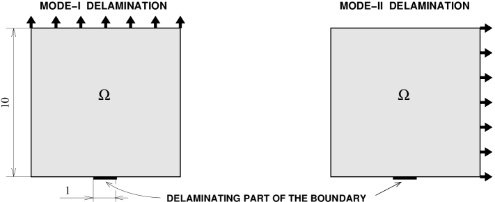
Figure 1: The square-shaped 2-dimensional domain $\varOmega$ and the boundary conditions: the mid-part of the bottom side where damageable Robin boundary conditions hold (i.e. the adhesive contact), traction boundary conditions are considered in the rest, either homogeneous or gradually increasing in time, considering two options leading primarily to Mode I and Mode II as depicted in the left and the right figure, respectively.

For mere demonstration of efficiency of the time/space discretisation and the algorithm, we take dimensionless data, i.e. without physical units. The material of the specimen considered here is assumed to be homogeneous and isotropic, with the bulk modulus $K{=}$1.66 and the shear modulus $G{=}$1. We further consider $\varrho=1$, which then corresponds to the pressure-wave velocity $v_{\rm p}=\sqrt{(K{+}4G/3)/\varrho}=\sqrt{3}=1.73$ and the shear-wave velocity $v_{\rm s}=\sqrt{G/\varrho}=1$.

The size of the square-shaped domain is as depicted in Figure 1. Namely, a square $\varOmega=(0,10)^{2}$ and the part of the boundary amenable to damage and thus debonding from an outer support is located at the center of the bottom boundary, cf. Fig. 1. Boundary conditions are of the form (1.5b) with $\mathchoice{{\buildrel\hskip 1.00006pt\text{\LARGE.}\over{g}}}{{\buildrel\hskip 1.00006pt\text{\Large.}\over{g}}}{{\buildrel\hskip 1.00006pt\text{\large.}\over{g}}}{{\buildrel\hskip 1.00006pt\text{\large.}\over{g}}}{=}0$ and the adhesive stiffness $\mathbb{B}=\frac{1}{2}\mathbb{I}$.

Furthermore, we took $\gamma(\alpha)=\alpha$ and considered the explicit constraints $0\leq\alpha\leq 1$, as mentioned in Sect. 5.4 as an alternative. The dissipation potential $\Psi$ of (2.3c) is taken like the former option in (5.17) with $\varepsilon_{1}=0$ and $\varOmega$ replaced by the delaminating part of $\varGamma$, and $\phi(\alpha)=\mathfrak{g}\alpha$ with the fracture-toughness constant $\mathfrak{g}{=}2.57\cdot 10^{-5}$.

The excitation is imposed on the loaded side by normal stresses assumed to vary linearly and slowly in time as σn=0.005t/Tsubscript𝜎𝑛0.005𝑡𝑇\sigma_{n}{=}0.005t/T, with T=51𝑇51T{=}51 being the total duration of the experiment. The tangent traction is assumed to be zero while, at the rest of the boundary, the traction-free boundary conditions are assumed and enforced. The computational experiments have
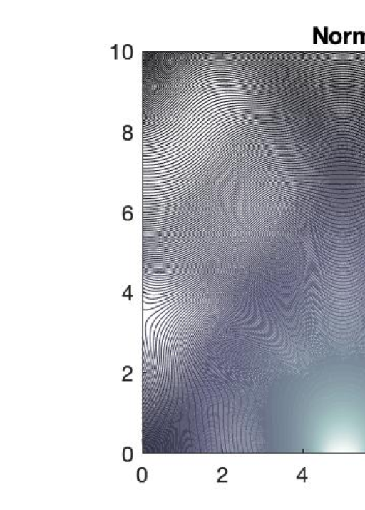
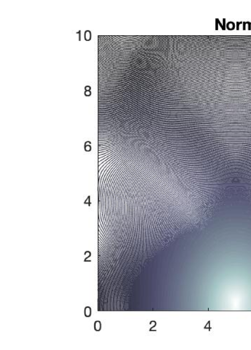
 been performed with the mesh size h=0.0250.025h{=}0.025, that gives a grid of 400×400400400400\times 400 elements. Thus, on adhesive-contact boundary, there are 404040 elements. The time discretisation step is Δt=1vph=0.0144Δ𝑡1subscript𝑣𝑝0.0144\Delta t=\frac{1}{v_{p}}h=0.0144.

The standard Helmholtz decomposition [2], usually used (e.g. in seismology [24]), is performed. The computed velocity gradient is therefore decomposed in its pressure and shear waves using $\nabla v=({\rm div}\,v){\mathbb{I}}/d+{\rm rot}\,v$.

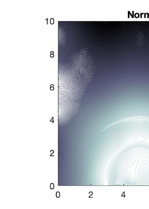
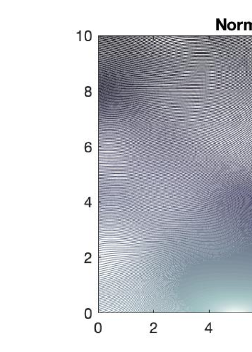
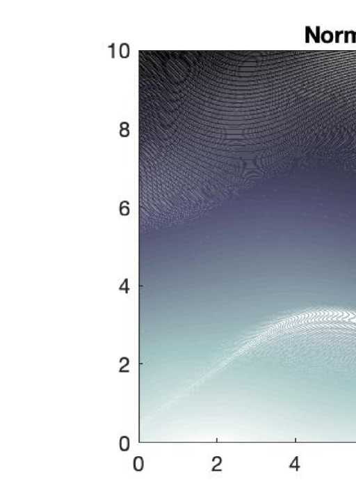
In the first experiment, the top side of the square-shaped domain is loaded as shown in Fig. 1(left). As it was expected a rather Mode-I debonding takes place. The acoustic emission generated by fast propagation of surface damage can be seen in Fig. 2 where the norm of the velocity vector field is plotted together with both the divergence and its rotational part to identify P-wave and S-wave, respectively. The term “acoustic emission” is used to describe the transient elastic waves caused by the rapid release of localized stress energy, but one can also understand it as a seismic-wave emission, depending on a particular application. This localization of the stress energy can be seen on the top row plots of Fig. 2 corresponding to time $t=20.2073$. Rupture is occurring rather rapidly during a very short time of successive symmetrical appeared damage events. Then elastic waves (both pressure and shear) emanate from the damaged region and propagate thorough the specimen as illustrated on selected snapshots at times $t=21.6506$, $t=23.094$, $t=23.8197$, and $t=24.630$ in Fig. 2.

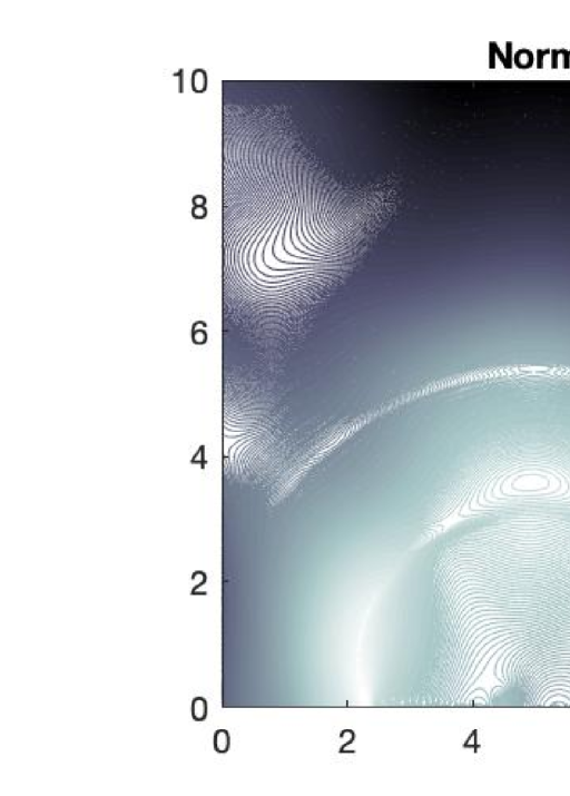
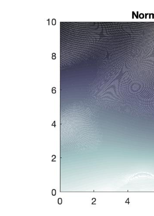
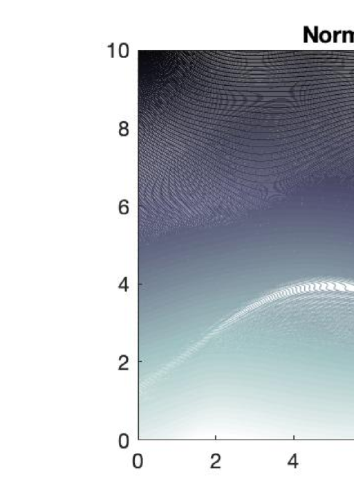
In the second experiment, a rather Mode-II damage evolution is performed by imposing the loading pattern of Fig. 1(right). In that case, a bit longer duration of time is needed for the damage to start expanding on the adhesive part of the boundary. The localization of the stress energy is illustrated on the top row plots of Fig. 3 corresponding to time $t=21.6506$. The rupture in this case consists of non symmetrical occurrences of damage events. The wave propagation of the velocity field can be seen in the plots of Fig. 3 with a more articulated S-wave while $P$-wave is rather suppressed.

In both experiments, the waves are quite sharp and nearly without spurious dispersion during their propagation. This shows efficiency of the explicit numerical algorithm even if combined with the dissipative inelastic process.

Refer to caption
Refer to caption
Refer to caption
Refer to caption
Refer to caption
Figure 2: Delamination (rather) in Mode I under the loading as in Fig. 1-left. Five selected time instants immediately after the delamination was executed are displayed in the following rows. Each row consist in spatial distribution of the norm of velocity, divergence of velocity, and rotation of velocity. Both P-wave and S-waves are emitted, the former one being faster, as clearly seen on the middle column.
Refer to caption
Refer to caption
Refer to caption
Refer to caption
Refer to caption
Figure 3: Delamination (rather) in Mode II under the loading as in Fig. 1-right. In the left column, it is clearly visible that the S-wave dominates.

Acknowledgments. Fruitful discussions with Dr. Radek Kolman are warmly acknowledged. This research has been partly supported from the grants 17-04301S (especially as far as the focus on the dissipative evolution of internal variables) and 19-04956S (especially as far as the focus on the dynamic and nonlinear behaviour) of the Czech Sci. Foundation. C.G.P. acknowledges the financial support of the Stavros Niarchos Foundation within the framework of the project ARCHERS (“Advancing Young Researchers’ Human Capital in Cutting Edge Technologies in the Preservation of Cultural Heritage and the Tackling of Societal Challenges”). T.R. also acknowledges the hospitality of (and partial support from) FORTH in Heraklion, Crete.

References

  • [1] Y.N. Abousleiman, A.H.-D. Cheng, and F.-J. Ulm, editors. Poromechanics III: Biot Centennial (1905–2005), London, 2005. Taylor & Francis.
  • [2] J. Achenbach. Wave propagation in elastic solids, volume 16. Elsevier, Amsterdam, 2012.
  • [3] L. Ambrosio and V. M. Tortorelli. Approximation of functional depending on jumps via by elliptic functionals via $\Gamma$-convergence. Comm. Pure Appl. Math., 43:999–1036, 1990.
  • [4] M. Arndt, M. Griebel, and T.Roubíček. Modelling and numerical simulation of martensitic transformation in shape memory alloys. Continuum Mech. Thermodyn., 15:463–485, 2003.
  • [5] E. Bécache, A. Ezziani, and P. Joly. A mixed finite element approach for viscoelastic wave propagation. Computational Geosciences, 8:255–299, 2004.
  • [6] E. Bécache, P. Joly, and C. Tsogka. Fictitious domains, mixed finite elements and perfectly matched layers for 2D elastic wave propagation. J. of Comput. Acoustics, 9(3):1175–1202, 2001.
  • [7] E. Bécache, P. Joly, and C. Tsogka. A new family of mixed finite elements for the linear elastodynamic problem. SIAM J. Numer. Anal., 39:2109–2132, 2002.
  • [8] M.A. Biot. General theory of three-dimensional consolidation. J. Appl. Phys., 12:155–164, 1941.
  • [9] T. Bohlen. Parallel 3-D viscoelastic finite difference seismic modelling. Computers & Geosciences, 28:887–899, 2002.
  • [10] M.J. Borden, C.V. Verhoosel, M.A. Scott, T.J.R. Hughes, and C.M. Landis. A phase-field description of dynamic brittle fracture. Comput. Meth. Appl. Mech. Engr., 217—-220:77–95, 2012.
  • [11] J.M. Carcione. Wave Fields in Real Media, Wave Propagation in Anisotropic, Anelastic, Porous and Electromagnetic Media. Elsevier, Amsterdam, 2015.
  • [12] A.H.-D. Cheng. Poroelasticity. Springer, Switzerland, 2016.
  • [13] E.T. Chung, C.Y. Lam, and J. Qian. A staggered discontinuous Galerkin method for the simulation of seismic waves with surface topography. Geophysics, 80:T119–T135, 2015.
  • [14] G. Cohen and S. Pernet. Finite Element and Discontinuous Galerkin Methods for Transient Wave Equations. Springer, Dordrecht, 2017.
  • [15] R. Courant, K. Friedrichs, and H. Lewy. Über die partiellen Differenzengleichungen der mathematischen Physik. Math. Annalen, 100:32–74, 1928.
  • [16] C.A. Felippa, K.C. Park, and C. Farhat. Partitioned analysis of coupled mechanical systems. Comput. Methods Appl. Mech. Engrg., 190:3247–3270, 2001.
  • [17] M. Frémond. Dissipation dans l’adhrence des solides. C. R. Acad. Sci., Paris, Sér.II, 300:709–714, 1985.
  • [18] R.W. Graves. Simulating seismic wave propagation in 3D elastic media using staggered-grid finite differences. Bull. Seismological Soc. Amer., 86:1091–1106, 1996.
  • [19] A.E. Green and P.M. Naghdi. A general theory of an elastic-plastic continuum. Arch. Rational Mech. Anal., 18:251–281, 1965.
  • [20] W. Han and B.D. Reddy. Plasticity. Springer, New York, 1999.
  • [21] M. Hofacker and C. Miehe. Continuum phase field modeling of dynamic fracture: variational principles and staggered FE implementation. Intl. J. Fract., 178:113–129, 2012.
  • [22] P. Joly and C. Tsogka. Finite Element Methods with Discontinuous Displacement, chapter 11. Chapman & Hall/CRC, Boca Raton, FL, 2008.
  • [23] L.M. Kachanov. Time of rupture process under creep conditions. Izv. Akad. Nauk SSSR, 8:26, 1958.
  • [24] A. Keiiti and P.G. Richards. Quantitative seismology. Univ. Sci. Books, Sausalito, CA, 2002.
  • [25] R. Kolman, J. Plešek, J. Červ, M. Okrouhlík, and P. Pařík. Temporal-spatial dispersion and stability analysis of finite element method in explicit elastodynamics. Intl. J. Numer. Meth. Engr., 106:113–128, 2016.
  • [26] J. Kopačka, A. Tkachuk, D. Gabriel, R. Kolman, M. Bischoff, and J. Plešek. On stability and reflection-transmission analysis of the bipenalty method in contact-impact problems: A one-dimensional, homogeneous case study. Int. J. Numer. Meth. Engng., 113:1–23, 2017.
  • [27] M. Kružík and T. Roubíček. Mathematical Methods in Continuum Mechanics of Solids. Springer, Switzeland, 2019. In print (ISBN 978-3-030-02064-4).
  • [28] G.A. Maugin. The saga of internal variables of state in continuum thermo-mechanics (1893-2013). Mechanics Research Communications, 69:79–86, 2015.
  • [29] A. Mielke and T. Roubíček. Rate-Independent Systems – Theory and Application. Springer, New York, 2015.
  • [30] S. Nilsson, N.A. Petersson, B. Sjögreen, and H.-O. Kreiss. Stable difference approximations for the elastic wave equation in second order formulation. SIAM J. Numer. Anal., 45:1902–1936, 2007.
  • [31] C.G. Panagiotopoulos, E.A. Paraskevopoulos, and G.D. Manolis. Critical assessment of penalty-type methods for imposition of time-dependent boundary conditions in FEM formulations for elastodynamics. In M. Papadrakakis, M. Fragiadakis, and N.D. Lagaros, editors, Computational Methods in Earthquake Engineering, pages 357–375. Springer, 2011.
  • [32] E. Paraskevopoulos, C. Panagiotopoulos, and D. Talaslidis. Rational derivation of conserving time integration schemes: the moving-mass case. In M. Papadrakakis, D.C. Charmpis, Y. Tsompanakis, and N.D. Lagaros, editors, Comput. Struct. Dynam. and Earthquake Engr., chapter 10, pages 149–164. CRC Press, Bocca Raton, 2009.
  • [33] E.A. Paraskevopoulos, C.G. Panagiotopoulos, and G.D. Manolis. Imposition of time-dependent boundary conditions in FEM formulations for elastodynamics: critical assessment of penalty-type methods. Computational Mechanics, 45:157, 2010.
  • [34] Yu.N. Rabotnov. Creep Problems in Structural Members. North-Holland, Amsterdam, 1969.
  • [35] T. Roubíček. Nonlinear Partial Differential Equations with Applications. Birkhäuser, Basel, 2nd edition, 2013.
  • [36] T. Roubíček. An energy-conserving time-discretisation scheme for poroelastic media with phase-field fracture emitting waves and heat. Disc. Cont. Dynam. Syst. S, 10:867–893, 2017.
  • [37] T. Roubíček, M. Kružík, V. Mantič, C.G. Panagiotopoulos, R. Vodička, and J. Zeman. Delamination and adhesive contacts, their mathematical modeling and numerical treatment. In V.Mantič, editor, Math. Methods and Models in Composites, chapter 11. Imperial College Press, 2nd edition.
  • [38] T. Roubíček and C.G. Panagiotopoulos. Energy-conserving time-discretisation of abstract dynamical problems with applications in continuum mechanics of solids. Numer. Funct. Anal. Optim., 38:1143–1172, 2017.
  • [39] T. Roubíček and R. Vodička. A monolithic model for phase-field fracture and waves in solid-fluid media towards earthquakes. Submitted.
  • [40] G. Scarella. Etude théorique et numérique de la propagation d’ondes en présence de contact unilatéral dans un milieu fissuré. PhD thesis, Univ. Paris Dauphine, 2004.
  • [41] A. Schlüter, A. Willenbücher, C. Kuhn, and R. Müller. Phase field approximation of dynamic brittle fracture. Comput Mech, 54:1141–1161, 2014.
  • [42] S. Seifi, K.C. Park, and H.S. Park. A staggered explicit-implicit finite element formulation forelectroactive polymers. Comput. Methods Appl. Mech. Engrg., 337:150–164, 2018.
  • [43] B. Straughan. Stability and Wave Motion in Porous Media. Springer, New York, 2008.
  • [44] R. Temam. Mathematical Problems in Plasticity. Gauthier-Villars, Paris, 1985. (French original in 1983).
  • [45] C. Tsogka. Modelisation mathématique et numérique de la propagation des ondes élastiques tridimensionnelles dans des milieux fissurés. PhD thesis, Univ. Paris IX Dauphine, 1999.
  • [46] J. Virieux. SH-wave propagation in heterogeneous media: Velocity-stress finite-difference method. Geophysics, 49:1933–1957, 1984.