Black-hole remnants from black-hole–neutron-star mergers

Abstract

Observations of gravitational waves and their electromagnetic counterparts may soon uncover the existence of coalescing compact binary systems formed by a stellar-mass black hole and a neutron star. These mergers result in a remnant black hole, possibly surrounded by an accretion disk. The mass and spin of the remnant black hole depend on the properties of the coalescing binary. We construct a map from the binary components to the remnant black hole using a sample of numerical-relativity simulations of different mass ratios $q$, (anti-)aligned dimensionless spins of the black hole $a_{\text{BH}}$, and several neutron star equations of state. Given the binary total mass, the mass and spin of the remnant black hole can therefore be determined from the three parameters $(q,a_{\text{BH}},\Lambda)$, where $\Lambda$ is the tidal deformability of the neutron star. Our models also incorporate the binary black hole and test-mass limit cases and we discuss a simple extension for generic black hole spins. We combine the remnant characterization with recent population synthesis simulations for various metallicities of the progenitor stars that generated the binary system. We predict that black-hole–neutron-star mergers produce a population of remnant black holes with masses distributed around $7M_{\odot}$ and $9M_{\odot}$. For isotropic spin distributions, nonmassive accretion disks are favoured: no bright electromagnetic counterparts are expected in such mergers.

Introduction.—

Mergers of a stellar-mass black hole (BH) and a neutron star (NS), hereafter BHNS, are expected sources of gravitational waves (GWs) detectable by ground-based laser-interferometers and possibly accompanied by electromagnetic counterparts Rosswog (2005); Kyutoku et al. (2011); Foucart et al. (2013, 2014, 2016); Paschalidis (2017); Bhattacharya et al. (2018). No GW observations of BHNS binaries have been made to date. The 90% confidence upper limit on their merger rate is $610~{}{\rm Gpc}^{-3}{\rm yr}^{-1}$ Abbott et al. (2018). To prepare these observations quantitative general-relativistic theoretical models of the GW and merger outcome are required.

Numerical-relativity (NR) simulations of BHNSs are the only means to study BHNS mergers Kyutoku et al. (2010, 2011, 2013, 2015); Foucart et al. (2011, 2013, 2014); Kawaguchi et al. (2015); Etienne et al. (2009, 2008, 2012a, 2012b); Paschalidis et al. (2013). Simulations indicated that the NS tidal disruption is a characteristic feature of the dynamics of quasi-circular BHNS mergers. On the contrary, quasi-circular binary NS mergers with mass ratio $q\lesssim 2$ do not present significant tidal disruption, e.g., Bejger et al. (2005); Dietrich et al. (2017). Physically, tidal disruption is expected if the binary reaches a characteristic radius $r_{\text{TD}}$ before the innermost stable circular orbit (ISCO), the radius of which we denote by $r_{\text{ISCO}}$. $r_{\text{TD}}$ is expected to scale in the same way as the mass-shedding radius $r_{\text{MS}}$, which is determined by the condition that the BH tidal force overcomes the NS self-gravity at the stellar surface $R_{\text{NS}}$: $r_{\text{TD}}\lesssim r_{\text{MS}}\propto q^{1/3}R_{\text{NS}}$, with a weak dependency on the BH spin Shibata and Taniguchi (2011). For a Kerr BH of mass $M_{\text{BH}}$, $r_{\text{ISCO}}=M_{\text{BH}}f(a_{\text{BH}})$, where $f(a_{\text{BH}})\in[1,9]$ is a monotonically decreasing function of the BH dimensionless spin parameter $a_{\text{BH}}$   Bardeen et al. (1972). Because $R_{\text{NS}}/M_{\text{BH}}=(qC)^{-1}$, where $C=M_{\text{NS}}/R_{\text{NS}}$ is the NS compactness, the ratio that regulates the onset of tidal disruption is $\xi=r_{\text{TD}}/r_{\text{ISCO}}\propto C^{-1}q^{-2/3}f(a_{\text{BH}})^{-1}$. Thus, tidal disruption depends on three physical parameters: the binary mass ratio, the BH spin and the NS compactness.

Simulations have shown that tidal disruption occurs for BHNSs with $q\lesssim 3$ if the BH is non-spinning, or its spin is anti-aligned with the orbital angular momentum. Generally speaking, large, aligned BH spins $a_{\text{BH}}\gtrsim+0.5$ favour tidal disruption because spin-orbit interactions push the ISCO radius to smaller values. As an example, $r_{\text{ISCO}}=1\,M_{\text{BH}}$ for a Kerr BH with $a_{\text{BH}}=+1$, as opposed to $r_{\text{ISCO}}=6\,M_{\text{BH}}$ for a non-spinning BH. Disruption is also favored by low values of the NS compactness, which are related to stiff equations of state, that also imply large NS tidal deformabilities Hinderer et al. (2010); Damour and Nagar (2010). Note that, for a fixed NS mass, large deformabilities imply large NS radii and small binary mass ratios correspond to small BH masses.

Figure 1: Contour plots of the remnant BH mass divided by the binary mass $X_{\bullet}=M_{\bullet}/M$ (top) and of the dimensionless spin parameter $a_{\bullet}$ (bottom) as a function of the symmetric mass ratio $\nu$ and of the NS tidal polarizability parameter $\Lambda$, at fixed values of the initial BH spin parameter $a_{\text{BH}}$. The values of $a_{\text{BH}}$ correspond to those of the NR simulations. White markers indicate the NR data used to construct the model.

Tidal disruption leads to the formation of an accretion disk in the merger remnant. Simulations predict remnant disks with baryon (rest) masses as large as $\gtrsim 0.1{\rm M_{\odot}}$ Foucart (2012); Foucart et al. (2018), thus creating the conditions to ignite a short gamma-ray burst (SGRB) Paczynski (1986); Eichler et al. (1989); Li and Paczynski (1998). Kyutoku et al. (2011) tentatively classify the phenomenology of BHNS mergers into three classes, based on the ratio $\xi$. For Type-I and Type-III mergers, tidal disruption occurs far from or close to the ISCO; for Type-II it does not occur and the NS plunges onto the BH, because the tidal disruption radius is located well within the ISCO. The three classes differ by their GW spectra and the disk masses. Type-II mergers are typically characterized by $q\gtrsim 3,~{}a_{\text{BH}}\lesssim 0$ and have a GW spectrum very similar to binary black holes (BBHs), e.g. Lackey et al. (2012); Pannarale et al. (2013, 2015a); Hinderer et al. (2016); Nagar et al. (2018).

An analytical formula for the BH remnant mass and dimensionless spin can be found using mass and angular momentum conservation arguments Pannarale (2013, 2014) (see also Buonanno et al. (2008)). That approach builds on estimates of the radiated energy and the binary orbital angular momentum based on the expressions for test particles on Kerr background at ISCO, and on the disk mass fits of Foucart (2012). Results are accurate to a few percent, which is comparable to the energy radiated in GWs. The largest uncertainty comes from the disk mass estimates in simulations e.g. Foucart et al. (2018); Radice et al. (2018).

In this work we model the remnant of BHNS using NR data. Using a state-of-art synthetic population we predict that the most likely BHNS mergers are of Type-II, leading to a population of light remnant BHs. Throughout this work we use geometric units $c=G=1$ unless otherwise stated.

Remnant mass and spin.—

Given the gravitational binary mass $M=M_{\text{BH}}+M_{\text{NS}}$, we map the remnant mass and spin parameters of BHNS mergers as follows:

$$F:(\nu,a_{\text{BH}},\Lambda)\to(X_{\bullet},a_{\bullet})\ .$$ (1)

where $X_{\bullet}=M_{\bullet}/M$ and $a_{\bullet}=S_{\bullet}/M_{\bullet}^{2}$, $M_{\bullet}$ and $S_{\bullet}$ being the mass and spin of the remnant BH, respectively. Above, $\nu=q/(1+q)^{2}\in[0,1/4]$ is the symmetric mass ratio ($q=M_{\text{BH}}/M_{\text{NS}}\geq 1$), spanning from the test-mass ($\nu=0$) to the equal-mass ($\nu=1/4$) limit. $a_{\text{BH}}$ is the dimensionless spin of the initial BH, that is aligned with the binary orbital angular momentum. The quantity $\Lambda$ is the NS quadrupolar tidal polarizability dimensionless parameter Hinderer et al. (2010), $\Lambda=2k_{2}/(3C^{5})$, where $k_{2}$ is the gravito-electric quadrupolar Love number, a monotonically decreasing function of the compactness $C$ Damour and Nagar (2010). $\Lambda$ describes tidal interactions at the leading order in post-Newtonian dynamics. Typically, $\Lambda\sim 100-2500$ for NS in BHNS systems, depending on the NS mass and equation of state (EOS).

We use data of NR simulations of quasi-circular BHNS mergers described in Kyutoku et al. (2010, 2011, 2015) and collected in the Supplementary Material (SM). These simulations adopt different neutron star matter EOSs and (anti-)aligned BH spin values.

The NS spin on the contrary is neglected and currently not accounted for in our models; however, this is expected to be a good approximation of realistic systems Bildsten and Cutler (1992); Kochanek (1992).

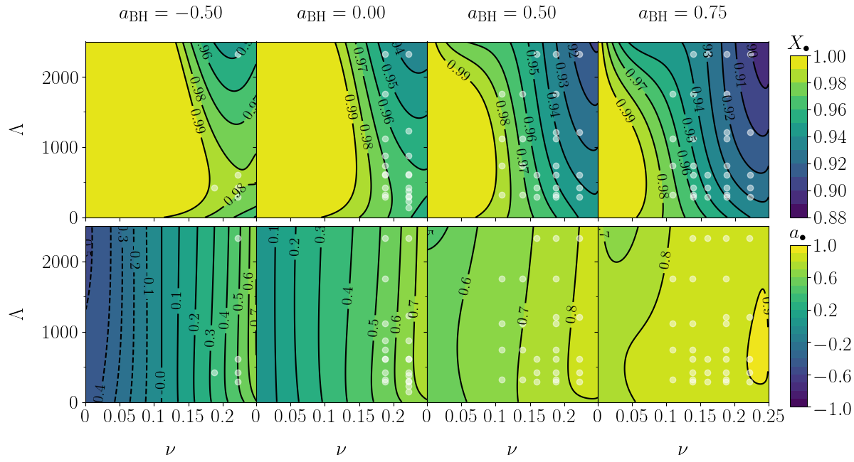
The data cover the following parameter intervals: $\Lambda\in[100,2500]$, $\nu\in[0.109,0.222]$, and $a_{\text{BH}}\in[-0.5,0.75]$. The mapping $F$ is summarized in Figure 1; technical details on its construction are provided in the SM.

The remnant BH mass scaled to $M$ is given by

$$X_{\bullet}=1-\frac{E_{\text{GW}}}{M}-\frac{M_{\text{disk}}}{M}\ ,$$ (2)

where $E_{\text{GW}}$ is the total energy radiated in GWs during the coalescence and $M_{\text{disk}}$ is the disk contribution to the gravitational energy which cannot be directly measured in the simulations . In BBH mergers finite mass-ratio effects are repulsive, implying that the GW emission is more efficient for larger $\nu$. The same effect is present in the BHNS dynamics: Figure 1 shows that the smallest values of $X_{\bullet}$ are obtained for larger values $\nu\to 1/4$. The precise behaviour of $X_{\bullet}$, however, depends on the competition between the energy emitted in GWs and the effect of tidal disruption, as per Eq. (2). For non-spinning BHNS binaries (second column in Figure 1), one observes that the value of $X_{\bullet}$ slightly increases with respect to the BBH case as $\Lambda>0^{+}$ and for a given $\nu$. Tidal disruption does not occur for small values of $\Lambda\sim 0$, so this effect is solely due to the fact that tidal interactions are attractive and reduce the emission of GWs with respect to the $\Lambda=0$ case (i.e., $E_{\text{GW}}$ decreases so $X_{\bullet}$ grows, with $M_{\text{disk}}\simeq 0$). As $\Lambda$ becomes sufficiently large (and $\nu\to 1/4$), tidal disruption occurs and only part of the remnant mass contributes to the final BH mass. Consequently, as $\Lambda$ increases beyond a certain critical value, $X_{\bullet}$ starts to decrease because part of the NS mass is not swallowed by the BH but becomes part of the disk. Note that the peak mass is more pronounced for $\nu\to 1/4$ and disappears for sufficiently small $\nu$ (Type-II mergers).

Focusing on spin effects, at a given $\nu$, the remnant mass decreases for increasing $a_{\text{BH}}>0$ because the ratio $\xi$ increases. This is a consequence of the repulsive character of the spin-orbit interaction for aligned (positive) spins. Notably, the peak for small $\Lambda$ is no longer present for sufficiently large values of $a_{\text{BH}}$. For $a_{\text{BH}}<0$, the spin-orbit interactions are attractive, i.e., they have the same sign as tidal interactions. As a consequence, for smaller $a_{\text{BH}}$’s, $X_{\bullet}$ increases and the peak at small $\Lambda$ is more pronounced.

For non-spinning BBHs, the remnant BH spin $S_{\bullet}$ is expected to decrease for increasing $\nu$, due to the same finite mass-ratio effect described above. Due to the $M^{2}_{\bullet}$ normalization, however, $a_{\bullet}$ shows the opposite behaviour. In the BHNS case, the remnant BH has a larger dimensionless mass-rescaled spin with respect to the BBH case and it increases with $\Lambda$, for small $\Lambda>0$. This happens because the NS compactness is smaller and less angular momentum is dissipated via GWs. Above a peak value, however, tidal disruption occurs and the angular momentum redistributes into the disk that forms around the remnant BH.

For $|a_{\text{BH}}|\lesssim 0.5$ and a given value of $\nu$, the final $a_{\bullet}$ is roughly linear in $a_{\text{BH}}$ [see Eq. (4) and Kyutoku et al. (2011)]. For $a_{\text{BH}}\gtrsim+0.75$, one recovers $a_{\bullet}\sim a_{\text{BBH}}$, as expected.

Although our models are developed from non-precessing BHNS data, they can be extended to the case of generic BH spins Barausse and Rezzolla (2009); Pannarale (2014); Hofmann et al. (2016). The simplest extension — which we adopt — is to map the initial spin

$$a_{\text{BH}}\rightarrow a_{\text{BH}}\cos\beta=a_{\text{BH}}^{z}\ ,$$ (3)

where $\beta$ is the angle between the initial BH spin and the orbital angular momentum L. In this case the model will yield $a_{\bullet}^{z}$ instead of $a_{\bullet}$. This prescription also assumes that the direction of the total angular momentum $\textbf{J}=\textbf{L}+\textbf{S}$ is approximately preserved and so the direction $\theta$ of the final spin is given by the projection $\cos\theta=\hat{\textbf{J}}\cdot\hat{\textbf{L}}$ . Predictions in the precessing case agree with the simulations of Kawaguchi et al. (2015), (see SM).

Figure 2: The remnant BH mass distribution inferred from the remnant to a different value of the metallicity $Z$ of the progenitor stars. In this plot we employ the SLy EOS and the fiducial isotropic spin distribution peaked around $\langle a_{\text{BH}}\rangle=0.2$.

Figure 3: Remnant disk baryonic mass distribution for different EOSs and for low (left) and high (right) aligned BH spin distributions. The mass threshold represents the minimum mass of the disk that allows the production of SGRBs with $1$ s duration. The percentage of binaries with disk mass bigger than the threshold is provided in the legend for each equation of state.

Binary and remnant population.—

We now apply the formalism described in the previous section to a BHNS population merging at redshift $z\leq{}1$ and constructed by convolving the binary population-synthesis from the mobse code Giacobbo et al. (2018); Giacobbo and Mapelli (2018, 2019) with the Illustris cosmological simulation (Vogelsberger et al. (2014a, b); Nelson et al. (2015), see Mapelli et al. (2017); Mapelli and Giacobbo (2018); Mapelli et al. (2019) and the SM for details). In particular, we adopt run CC15$\alpha{}5$ of Mapelli et al. (2019) where the common-envelope parameter is $\alpha{}=5$ and natal kicks are drawn from a Maxwellian distribution with a single root-mean square velocity $v_{\sigma}=15$ km s^-1 for both electron-capture and core-collapse supernovae. Larger kicks would enable the merger of more massive BHNSs (moderate kicks do not break the binary but increase its eccentricity, shortening the merger time of massive BHNSs, see Giacobbo and Mapelli (2018) for details), but would not affect the minimum BHNS mass (See Figure 5 of Mapelli et al. (2019)). In run CC15$\alpha{}5$, the minimum (maximum) mass of a BH (NS) is set to 5 (2) $M_{\odot}$. This assumption enforces the existence of a mass gap between BHs and NSs, which is suggested by dynamical mass measurements of compact objects in X-ray binaries Özel et al. (2010); Farr et al. (2011). BH spins are added by randomly drawing spin magnitudes $|a_{\text{BH}}|\in[0,1]$ from a truncated Maxwellian distribution with root mean square $\sigma{}$. In this paper, we consider spins isotropically oriented with respect to the binary orbital plane with $\langle a_{\text{BH}}\rangle=0.2$ as fiducial distribution or aligned spin distributions with $\sigma{}=(0.1,0.35,0.5,0.7)$, corresponding to average values $\langle a_{\text{BH}}\rangle=(0.2,0.5,0.75,0.95)$. The aligned spin distributions give upper limits to the isotropic spin distributions.

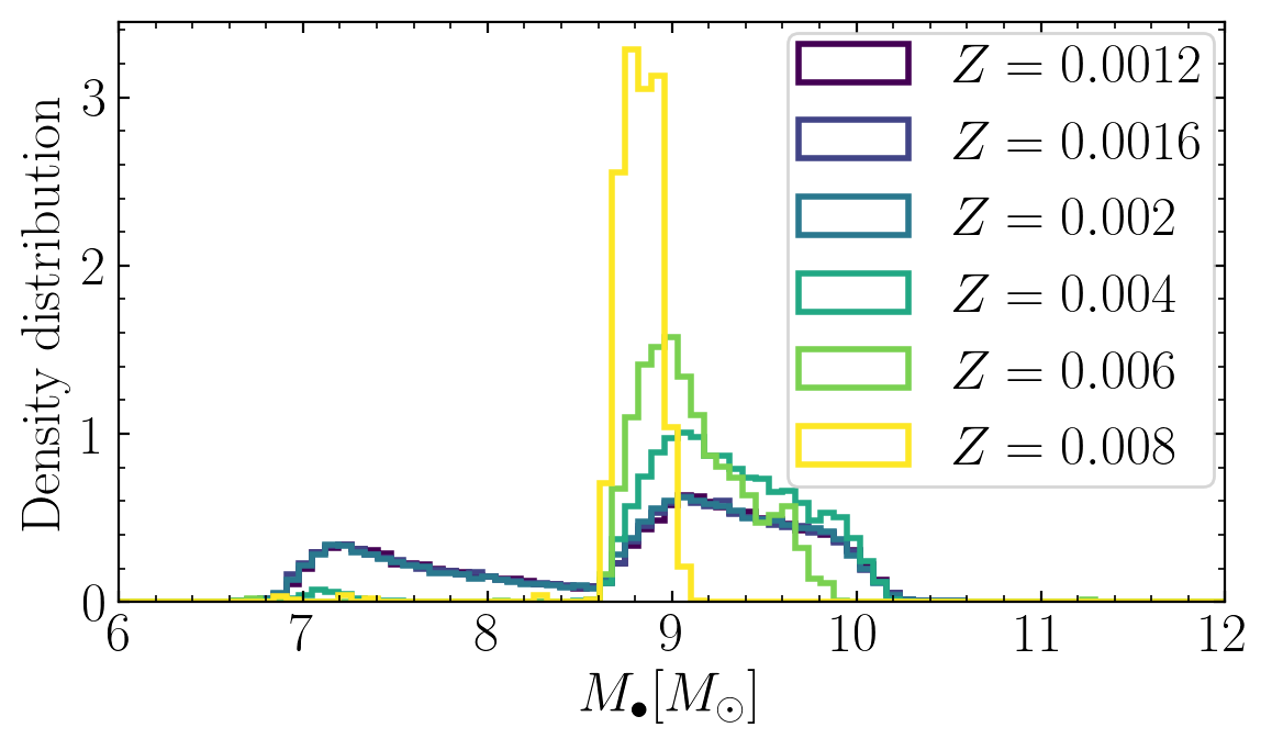
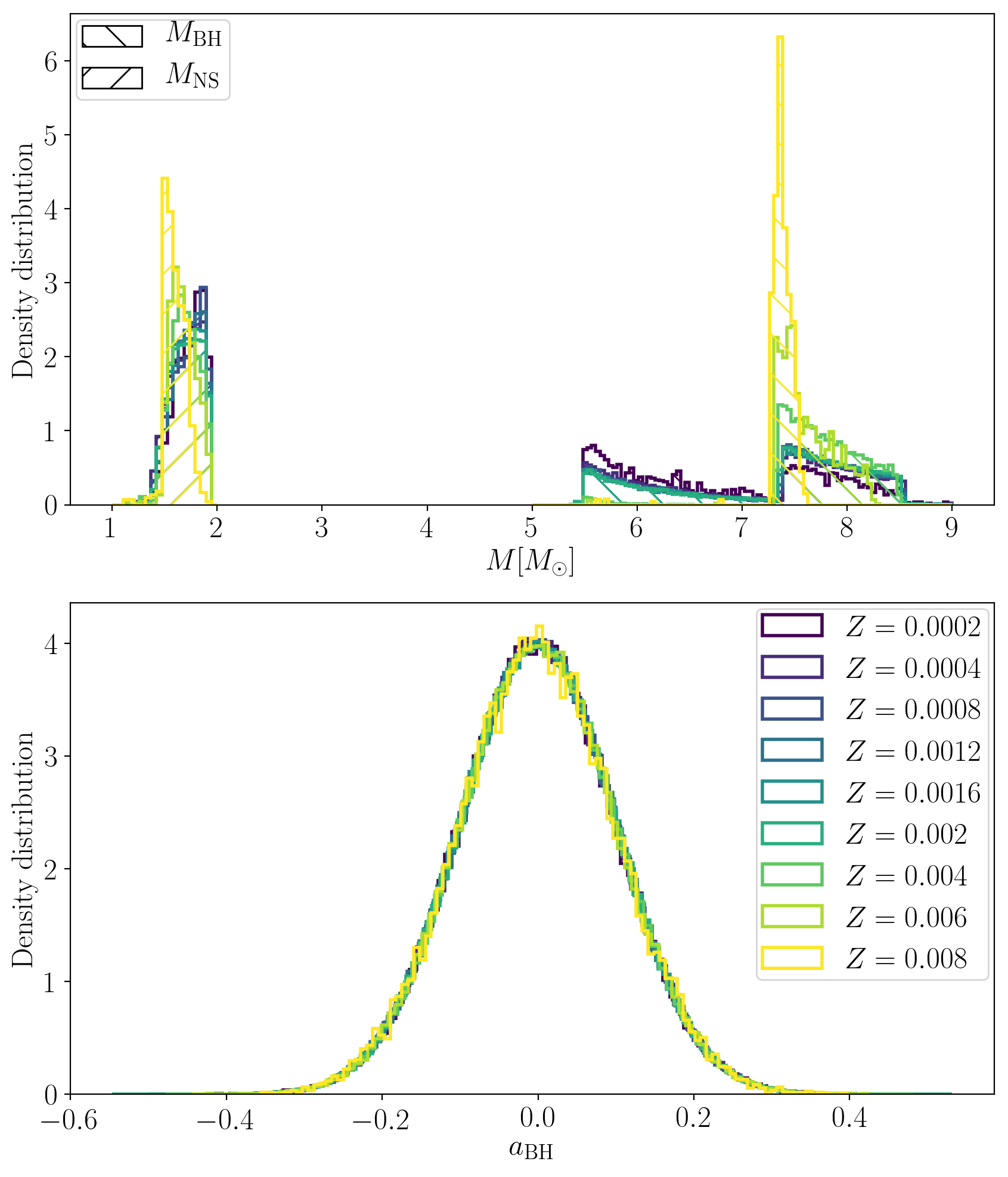
The population synthesis predicts BH component masses bellow $10{\rm M_{\odot}}$ distributed narrowly about $M_{\text{BH}}\sim 5{\rm M_{\odot}}$ and $M_{\text{BH}}\sim 8{\rm M_{\odot}}$ Mapelli and Giacobbo (2018). The population depends very weakly on progenitors’ metallicities for $Z\leq 0.002$, but for $Z\geq 0.003$ the smallest BHs are suppressed and only BH with $M_{\text{BH}}\sim 8{\rm M_{\odot}}$ are found. This is a consequence of the dependence of the delay time (i.e., the time elapsed between the formation of the progenitor stars and the BHNS merger) on the progenitor’s metallicity: metal-rich progenitors have longer delay times than metal-poor ones and thus do not merge within the Hubble time, especially if the BH mass is small [Giacobbo et al., In prep.]. Additionally, NS masses $M_{\text{NS}}\gtrsim 1.3{\rm M_{\odot}}$ are favoured.

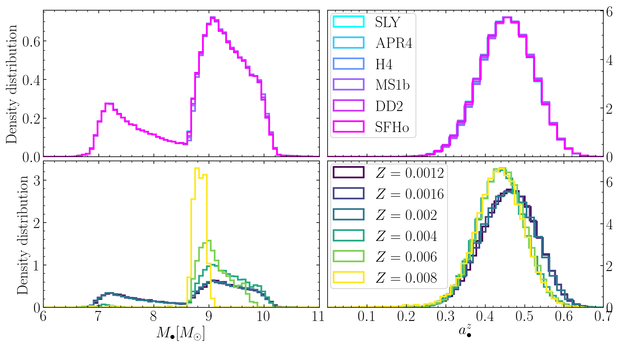
In order to compute the merger remnant from the population, we choose a representative set of EOSs, and calculate $\Lambda$ on the NS population for each EOS. The remnant properties are then determined with Eq. (1) with the prescription of Eq. (3). Remnant masses are shown in Figure 2, while additional plots are reported in the SM. For metallicities $Z\leq 0.002$, we find a bimodal distribution around $M_{\bullet}\sim 7{\rm M_{\odot}}$ and $M_{\bullet}\sim 9{\rm M_{\odot}}$ independently from the EOS. Large metallicities produce only the more massive remnants. The remnant spins inferred from Eq. (1) and the isotropic/aligned spin population with $\langle a_{\text{BH}}\rangle\approx 0.2$ are distributed around $a_{\bullet}^{z}\sim 0.4$ with standard deviation $\sim 0.1$.

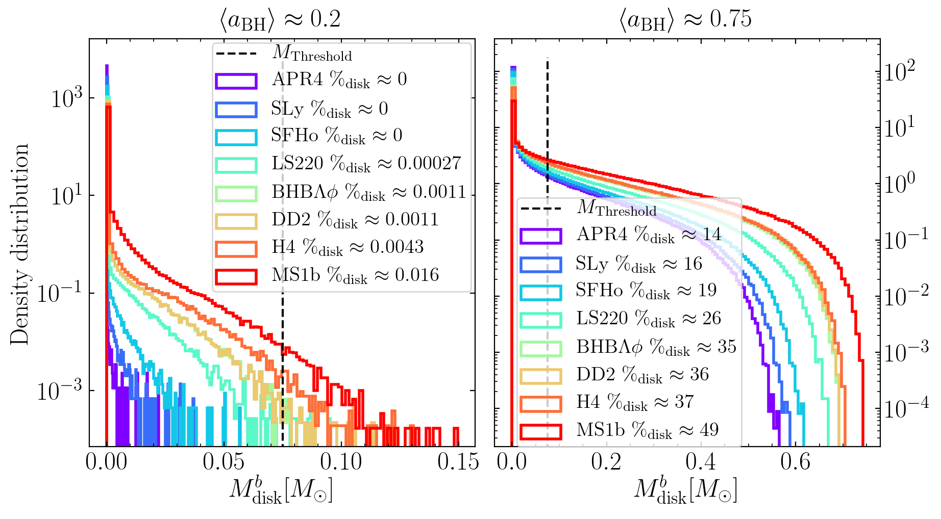
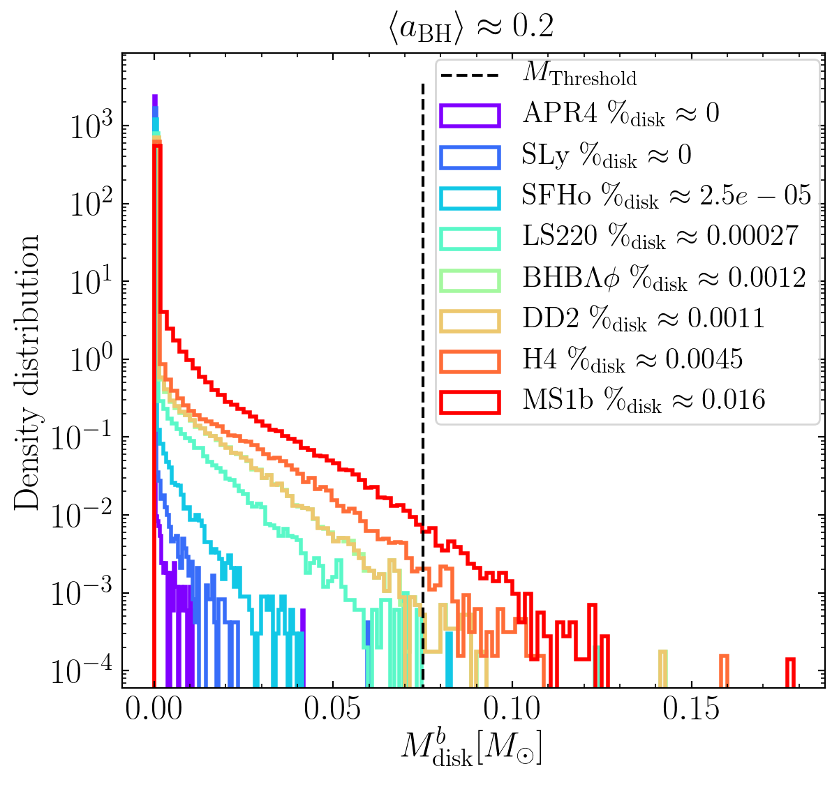
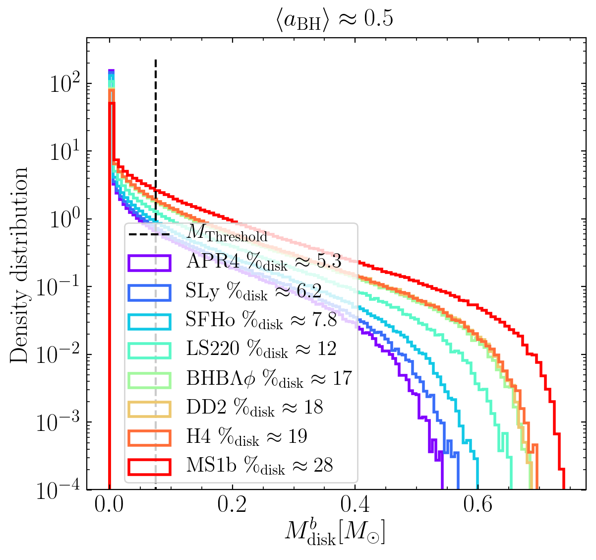
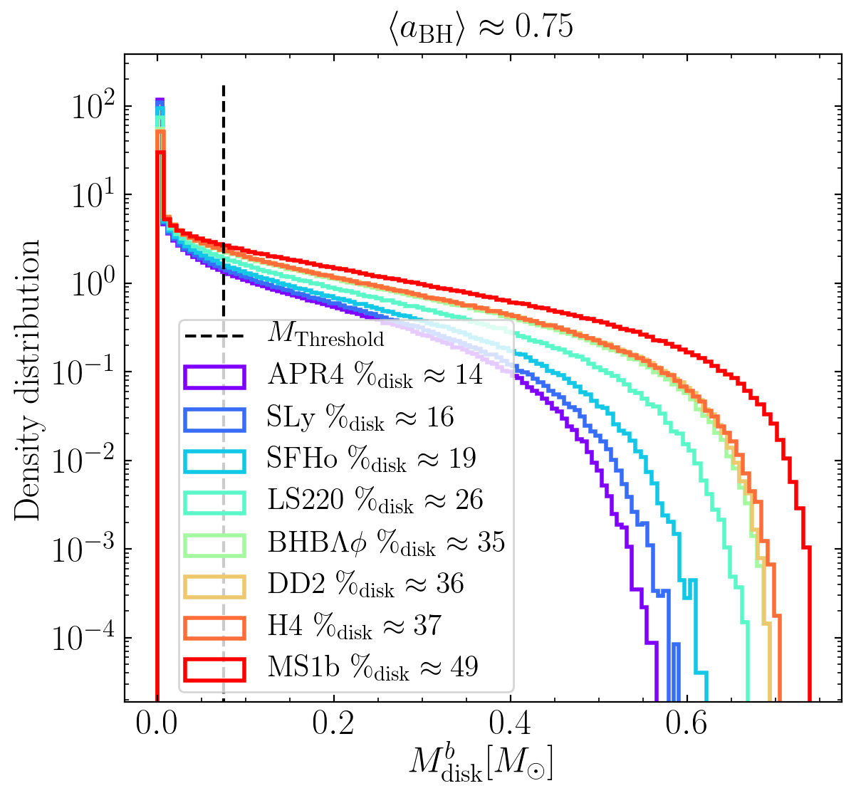
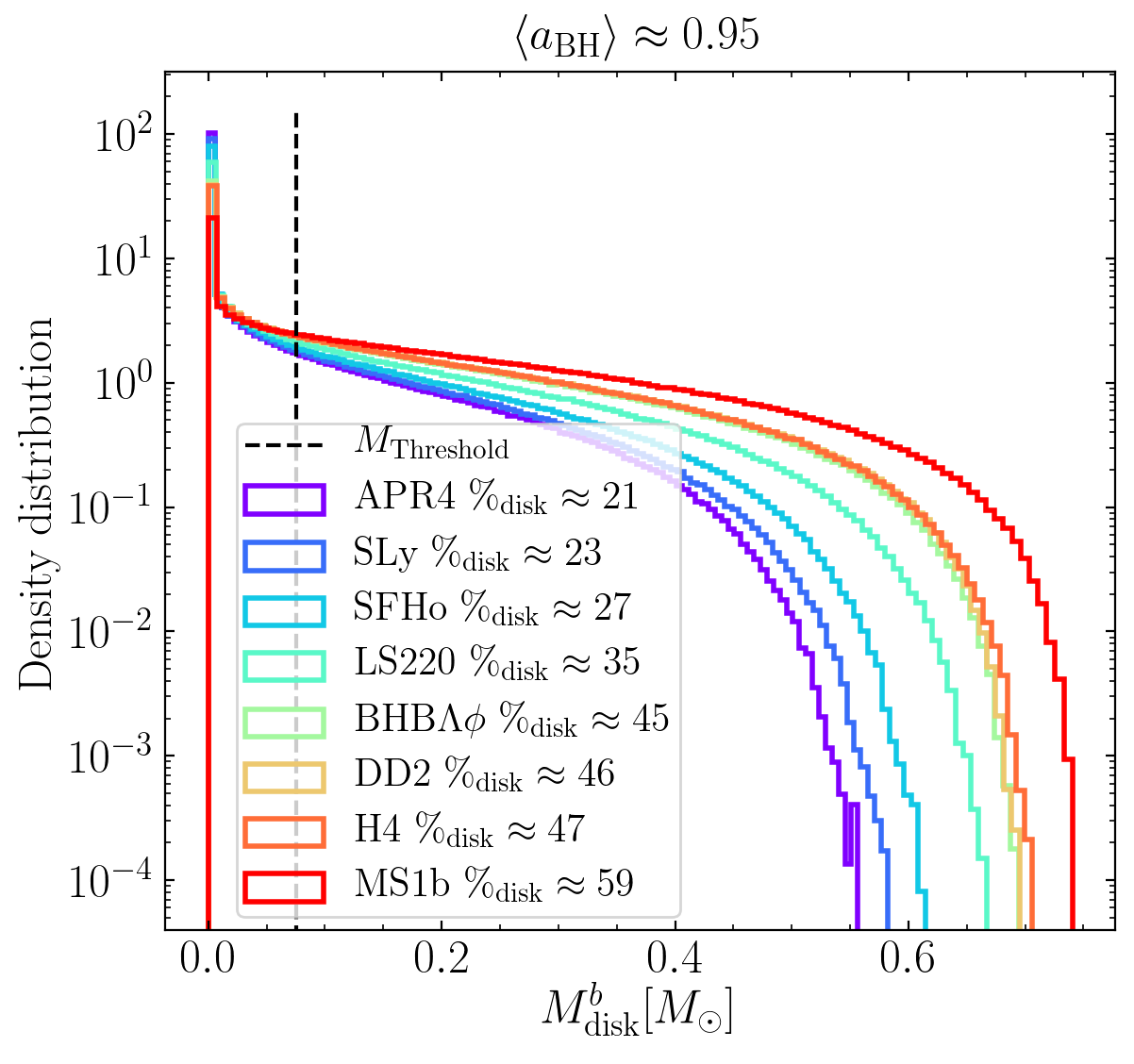
Using the model of Foucart et al. (2018), we estimate the baryonic mass of the remnant disk. Figure 3 shows the aligned low spin distribution resulting in $\gtrsim 99\%$ of the remnants with baryonic mass of the disk smaller than $M^{b}_{\text{Threshold}}=0.075(M_{\text{NS}}^{b}/1.5){\rm M_{\odot}}$ independently from the EOS. Disk masses above $M^{b}_{\text{Threshold}}$ are necessary to produce SGRBs of $1$ s duration Stone et al. (2013); Pannarale and Ohme (2014). Remnants with significant disk masses are found for aligned spin distributions with $\langle a_{\text{BH}}\rangle\gtrsim 0.5$. In these cases, the largest disks are found for the stiff EOS corresponding to $\Lambda\gtrsim 1700$. Soft EOS, corresponding to $\Lambda\lesssim 400$, give massive disks only for $\lesssim 20\%$ of the binaries and with $\langle a_{\text{BH}}\rangle\gtrsim 0.75$.

Conclusion.—

Our results indicate light and moderately spinning BH remnants surrounded by low-mass accretion disks (Type-II) as the most likely outcome for BHNS if $\Lambda\lesssim 1000$ and the BH has aligned spin $a_{\text{BH}}\lesssim 0.75$. The observation of GW170817 rules out NS with $\Lambda\gtrsim 1800$ ($\gtrsim 2600$) for the low- (high-) spin prior cases Abbott, B. P. and others (2019). Similarly, large aligned spins might be disfavoured by current GW binary observations Abbott et al. (2018). Type-II GW signals are very similar to BBHs. For aligned spins, GW searches will lose less than 1% of events employing BBH templates Harry et al. (2016). On the other hand, estimating $\Lambda$ from the GW will be challenging, and BHNS mergers might not set constraints on the EOS unless ringdown signatures are resolved Pannarale (2013). Type-II mergers are also not expected to be accompanied by bright electromagnetic counterparts. Disk masses above $M^{b}_{\text{Threshold}}$ are rare in our populations, unless BHNSs are characterized by large and aligned BH initial spins, very stiff EOS and/or compact objects with mass $2-5\,{}M_{\odot}$ (i.e. within the mass gap suggested by X-ray binaries).

The BH remnant model constructed in this work will be used in GW models for BHNSs Lackey et al. (2012, 2014); Pannarale (2014); Pannarale et al. (2015a, b); Hinderer et al. (2016); Nagar et al. (2018), as well as for modeling the counterparts, e.g. Lee et al. (2000); Beloborodov (2000); Kawaguchi et al. (2016); Perego et al. (2017); Barbieri et al. (2019). It will thus be one of the key building blocks for upcoming multi-messenger analysis of BHNSs.

Supplementary Materials

I Data and model construction

We construct a model for the mass and spin of the remnant BH based on the following expression

$$F(\nu,a_{\text{BH}},\Lambda)=F_{\text{BBH}}(\nu,a_{\text{BH}})\frac{1+p_{1}(\nu,a_{\text{BH}})\Lambda+p_{2}(\nu,a_{\text{BH}})\Lambda^{2}}{\left(1+[p_{3}(\nu,a_{\text{BH}})]^{2}\Lambda\right)^{2}}\ ,$$ (4)

where $F_{\text{BBH}}$ are the BBH models for mass and spin developed in Jiménez-Forteza et al. (2017) and $p_{k}(\nu,a_{\text{BH}})$ are polynomials of the form

$$p_{\rm k}(\nu,a_{\text{BH}}) =p_{k1}(a_{\text{BH}})~{}\nu+p_{k2}(a_{\text{BH}})~{}\nu^{2}$$ (5)

$$p_{kj}(a_{\text{BH}}) =p_{kj0}~{}a_{\text{BH}}+p_{kj1}\ .$$ (6)

The model includes by construction the BBH limit for $\Lambda\rightarrow 0$ (no tidal effects) and the test-mass limit for $\nu\rightarrow 0$. Note that the dependence on BH spin is linear. The coefficient $p_{3}(\nu,a_{\text{BH}})$ is squared in order to avoid a pole in the denominator.

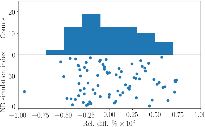
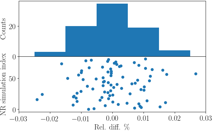
The NR data used for our work is collected in LABEL:tab:data. The values of the best-fit parameters $p_{kjl}$ are reported in Table 1; relative differences with respect to the fit are shown in Figure 4. The fits have determination coefficient $R^{2}\sim 0.92$ and the residuals are normally distributed with mean $\sim 0$ and standard deviations $\sim 0.25\times 10^{-2}$ and $\sim 0.01$, respectively. The maximum relative differences are below $1\%$ for the remnant mass fit and below $3\%$ for the the remnant spin; hence, fit uncertainties are smaller than NR errors. The NR data do not extend to $\nu\lesssim 0.1$ and $a_{\text{BH}}\lesssim-0.5\vee a_{\text{BH}}\gtrsim 0.75$, thus the model effectively extrapolates into those regions. The extrapolation leads in some cases to unphysical values of $X_{\bullet}>1$ and $a_{\bullet}<-1$. This behaviour is fixed by forcing the model to agree with the BBH, i.e., forcing $X_{\bullet}=1$ and $|a_{\bullet}|\leq 1$. We expect that future calibration of the model with new NR data will improve the behaviour for large mass ratios. We stress that BHNSs with mass ratios $q\gtrsim 7$ are in any case effectively indistinguishable from BBHs.

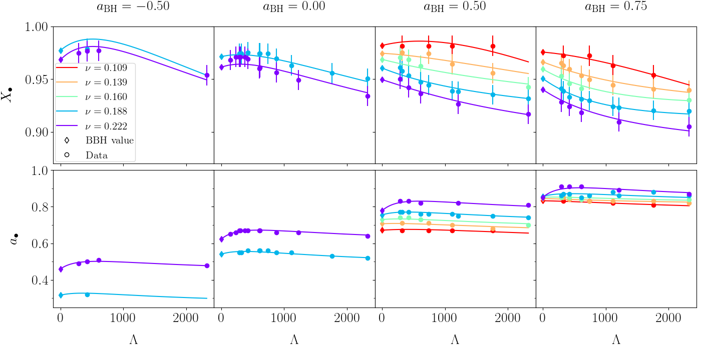
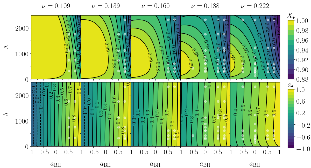
Figure 5 and Figure 6 complement Figure 1 in the main text. Figure 5 shows the model dependencies on $\Lambda$ for each given value of $a_{\text{BH}}$. We show NR errors in the plot, optimistically taken to be at the $1\%$ level. Note that in the final spin plot the errorbars are smaller than the markers. The contour plots in Figure 6 show the model evaluated on the entire parameter space (the plots in the main section of the paper are here reproduced for completeness).

Table 1: Best fit parameters of the remnant model for mass, spin and peak luminosity and the respective determination coefficient $R^{2}$ of the fit.

$F$	$k$	$p_{k10}$	$p_{k11}$	$p_{k20}$	$p_{k21}$	$R^{2}$
	$1$	$-1.83\times 10^{-3}$	$2.39\times 10^{-3}$	$4.29\times 10^{-3}$	$9.8\times 10^{-3}$
$X_{\bullet}$	$2$	$2.34\times 10^{-7}$	$-8.28\times 10^{-7}$	$-1.64\times 10^{-6}$	$8.08\times 10^{-6}$	$0.921$
	$3$	$-2.01\times 10^{-2}$	$1.32\times 10^{-1}$	$6.51\times 10^{-2}$	$-1.43\times 10^{-1}$
	$1$	$-5.44\times 10^{-3}$	$7.91\times 10^{-3}$	$2.33\times 10^{-2}$	$2.48\times 10^{-2}$
$a_{\bullet}$	$2$	$-8.57\times 10^{-7}$	$-2.82\times 10^{-6}$	$6.61\times 10^{-6}$	$4.29\times 10^{-5}$	$0.92$
	$3$	$-3.04\times 10^{-2}$	$2.55\times 10^{-1}$	$1.48\times 10^{-1}$	$-4.28\times 10^{-1}$
	$1$	$3.08\times 10^{-2}$	$-4.18\times 10^{-2}$	$-5.17\times 10^{-2}$	$3.19\times 10^{-1}$
$L_{\text{peak}}$	$2$	$-1.23\times 10^{-5}$	$8.84\times 10^{-6}$	$1.05\times 10^{-4}$	$-3.88\times 10^{-5}$	$0.98$
	$3$	$3.30\times 10^{-1}$	$-3.76\times 10^{-2}$	$-9.2\times 10^{-1}$	$1.44$

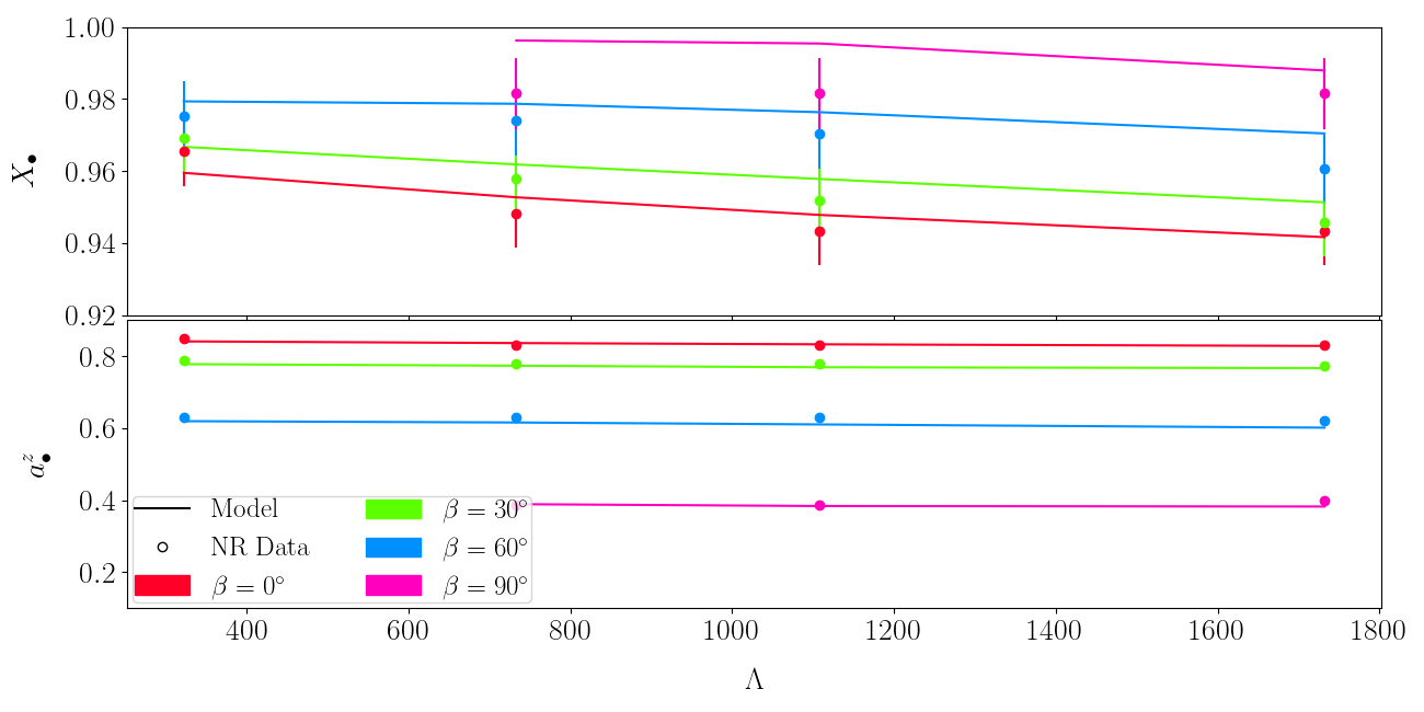
Finally, we validate the prescription used to extend the model to spin precessing cases. Figure 7 shows the agreement between the model predictions for $X_{\bullet}$ and $a_{\bullet}$ using Eq. (3) and the NR data of Kawaguchi et al. (2015) (not used to determine the model).

Figure 4: Relative differences of the data points to the fit. Left panel: $X_{\bullet}$, the maximum difference is of the order of $1\%$. Right panel: $a_{\bullet}$, the maximum difference is below $3\%$. In both cases the coefficient of determination of the fit is $R^{2}\sim 0.92$.

Figure 5: The remnant BH fractional mass $X_{\bullet}=M_{\bullet}/M$ (top) and dimensionless spin parameter $a_{\bullet}$ (bottom) as a function of the tidal polarizability parameter $\Lambda$ at given values of the initial BH spin parameters $a_{\text{BH}}$. The values of $a_{\text{BH}}$ correspond to those of the NR simulations.

Figure 6: Top: Contour plots of the remnant BH fractional mass $X_{\bullet}=M_{\bullet}/M$ and dimensionless spin parameter $a_{\bullet}$ as functions of the symmetric mass ratio $\nu$ and the NS tidal polarizability parameter $\Lambda$ at given values of the initial BH spin parameters $a_{\text{BH}}$. The values of $a_{\text{BH}}$ correspond to those of the NR simulations. Bottom: The same physical quantities are shown as functions of the initial BH spin parameters $a_{\text{BH}}$ and the NS tidal polarizability parameters $\Lambda$ at given values of the symmetric mass ratio $\nu$. The values of $\nu$ correspond to those of the NR simulations. White markers indicate the NR data used to construct the model.

Figure 7: Model performance for binaries with spin-precession. The model is validated against the numerical data of Kawaguchi et al. (2015). $\beta$ is the angle between the initial orbital angular momentum and the initial BH spin. Note that the exact values of $\beta$ are slightly different from the ones reported here, as explained in the reference. All these data correspond to fixed values of $(a_{\text{BH}},q)=(0.75,5)$ and the errorbars are taken as a $1\%$ of the values.

II GW peak luminosity

Figure 8: Distribution of the GW peak luminosity as a function of the NS $\Lambda$ for all the values of $a_{\text{BH}}$ and for all the different values of $\nu$.

The approach used in this paper can be used to estimate the GW peak luminosity, thus complementing the result derived for BBHs and binary NS systems in Keitel et al. (2017); Zappa et al. (2018) (see Abbott et al. (2018) for an application of those results). The GW peak luminosity is computed from the $(2,2)$ mode of the GW strain,

$$L_{\text{peak}}=\max_{t}\frac{1}{16\pi}\left(\left|\frac{dh_{22}(t)}{dt}\right|^{2}\right)$$ (7)

where

$$h_{+}-ih_{\times}=\sum_{\ell,m}h_{\ell m}(t){}^{-2}Y_{\ell,m}\approx h_{22}(t)({}^{-2}Y_{2,2}+{}^{-2}Y_{2,-2})\ ,$$ (8)

and ${}^{-2}Y_{\ell,m}$ are the spin-weighted $s=-2$ spherical harmonics.

Figure 8 shows the peak luminosity model as a function of $\Lambda$ and for the values of $\nu$ and $a_{\text{BH}}$ sampled by the NR dataset. The behaviour of $L_{\text{peak}}$ closely mirrors the one for $X_{\bullet}$ detailed in the main text. The model for $L_{\text{peak}}$ is slightly different from Eq. (4); in order to avoid negative, unphysical values we fit the ansatz

$$L_{\text{peak}}(\nu,a_{\text{BH}},\Lambda)=L_{\text{peak\, BBH}}(\nu,a_{\text{BH}})\frac{\left(1+p_{1}(\nu,a_{\text{BH}})\Lambda+p_{2}(\nu,a_{\text{BH}})\Lambda^{2}\right)^{2}}{\left(1+[p_{3}(\nu,a_{\text{BH}})]^{2}\Lambda\right)^{4}}\ .$$ (9)

The best parameters $p_{kjl}$ are reported in Table 1. The model delivers results accurate at the $20\%$ level.

The python code which implements these models is available at https://git.tpi.uni-jena.de/core/bhnsremnant.

III Synthetic population

The BHNS population is constructed from the results of the binary population-synthesis code mobse Giacobbo et al. (2018); Giacobbo and Mapelli (2018, 2019) convolved with the Illustris cosmological simulation Vogelsberger et al. (2014a, b); Nelson et al. (2015), and following the Monte Carlo method already described in Mapelli et al. (2017); Mapelli and Giacobbo (2018). mobse includes up-to-date prescriptions for stellar winds (accounting for the stellar metallicity and luminosity dependence of the mass loss), core-collapse supernovae (SNe), electron-capture SNe and (pulsational) pair instability SNe (see Giacobbo and Mapelli (2018) for more details). The interface with the Illustris simulation enables us to know the merger redshift of each simulated BHNS (see Mapelli and Giacobbo (2018)). We consider only BHNSs merging at redshift $z\leq{}1$.

Here, we adopt run CC15$\alpha{}5$ discussed in Mapelli et al. (2019). In this run, we fix common-envelope parameter $\alpha{}=5$ and we draw natal kicks from a Maxwellian distribution with one root-mean square velocity $v_{\sigma}=15$ km s^-1 for both electron-capture and core-collapse SNe. Larger kicks would enable the formation of few more massive BHNSs, but would not affect the minimum BHNS mass (see Figure 5 of Mapelli et al. (2019)). The minimum (maximum) mass of a BH (NS) in run CC15$\alpha{}5$ is set to 5 (2) $M_{\odot}$ (see the rapid model in Fryer et al. (2012) for details). This assumption enforces the existence of a mass gap between BHs and NSs, which is mildly suggested by dynamical mass measurements of compact objects in X-ray binaries Özel et al. (2010); Farr et al. (2011).

BH spins are added in post-processing through a toy model as there is no commonly accepted model to derive BH spins from the properties of their stellar progenitors. We randomly assign BH spin magnitudes $0\leq{}|a_{\text{BH}}|\leq{}1$ from a truncated Maxwellian distribution with one-dimensional root mean square $\sigma{}$. For the analysis of the remnant black hole distribution we assume spins isotropically oriented with respect to the binary orbital plane with modulus $\langle a_{\text{BH}}\rangle\approx 0.2$ using the prescription for precessing binaries described in the main text. In the disk analysis, by contrast, we consider different aligned spin distributions with $\sigma{}=(0.1,0.35,0.5,0.7)$ corresponding to means $\langle a_{\text{BH}}\rangle=(0.2,0.5,0.75,0.95)$ because the forumlae we use to estimate the disk mass are developed for aligned black hole spins. However, the aligned spin distributions give upper limits to the isotropic spin distributions. We assume all NSs have zero spins.

Figure 9 shows the distribution of the BHNS parameters, while Figure 10 shows the distribution of the remnant masses and spins derived from them. Finally, Figure 11 gives an overview of the disk analysis considering different distributions of aligned spins. The disk rest mass is calculated using the model of Foucart et al. (2018). For the aligned low-spin distribution with $\langle a_{\text{BH}}\rangle=0.2$ no massive disk is formed independently from the EOS. An analogous result is obtained for our fiducial isotropic spin distributions (not shown). For the aligned spin distribution with $\langle a_{\text{BH}}\rangle=0.5$, stiff EOSs give massive disks in $\lesssim 20\%$ of the cases. Note that the MS1b EOS is ruled out by the GW170817 analysis (low-spin priors), while H4 and DD2 are consistent with it. Aligned spins populations with $\langle a_{\text{BH}}\rangle\gtrsim 0.75$ yield more massive disks. Soft EOSs such as APR and SLy admit massive disks in about $\lesssim 20\%$ of the binaries only if $\langle a_{\text{BH}}\rangle\gtrsim 0.95$.

Figure 9: Distribution of initial component masses of the BHNS systems from population synthesis simulations (top panel) and initial BH spin (bottom panel) for different metallicities.

Figure 10: Final BH mass distribution (left) and final BH spin distribution (right) for different equations of state (top panels) and for different metallicities (bottom panels). Note that the prescription for precessing BHs is employed and so the $z-$component of the spin is reported. In this plot we employ the fiducial isotropic spin distribution peaked around $\langle a_{\text{BH}}\rangle=0.2$ and the SLy EOS is used in the bottom panels.

Figure 11: Baryonic mass distributions of the remnant disk for different equations of state and under the assumption of aligned BH spins. The mass threshold represents the minimum mass of the disk that allows the production of SGRBs with $1$ s duration. Each panel corresponds to a distribution of the initial BH spin peaked around the value reported on top. The percentage of binaries with disk mass bigger than the threshold is given in the legend for each EOS. These results have to be considered upper limits to the isotropic spins case.

Table 2: Numerical relativity simulation data. $M\Omega_{0}$ refers to the initial orbital frequency of the binary system, multiplied by the total mass of the binary system, while the other quantities have already been introduced in the first two paragraphs of the paper. For some simulations we did not have the final mass and spin of the remnant black hole (dashes in the table), but we could employ them to determine the fitting formula for $L_{\text{peak}}$.

Name	EOS	$q$	$\nu$	$M_{\text{NS}}$	$a_{\text{BH}}$	$M\Omega_{0}$	$C$	$M$	$k_{2}$	$\Lambda$	$X_{\bullet}$	$a_{\bullet}$	$L_{\text{peak}}$
2H-Q2M135a75	2H	2	0.222	1.35	0.75	0.0250	0.1309	4.05	0.1342	2327	0.9049	0.87	2.574e-05
1.5H-Q2M135a75	1.5H	2	0.222	1.35	0.75	0.0280	0.1456	4.05	0.1190	1212	0.9094	0.89	5.002e-05
H-Q2M135a75	H	2	0.222	1.35	0.75	0.0280	0.1624	4.05	0.1031	608	0.9183	0.91	9.808e-05
HB-Q2M135a75	HB	2	0.222	1.35	0.75	0.0280	0.1718	4.05	0.0950	423	0.9242	0.91	1.400e-04
B-Q2M135a75	B	2	0.222	1.35	0.75	0.0280	0.1819	4.05	0.0863	288	0.9282	0.91	1.974e-04
2H-Q2M135a5	2H	2	0.222	1.35	0.50	0.0250	0.1309	4.05	0.1342	2327	0.9168	0.81	2.798e-05
1.5H-Q2M135a5	1.5H	2	0.222	1.35	0.50	0.0280	0.1456	4.05	0.1190	1212	0.9262	0.82	5.481e-05
H-Q2M135a5	H	2	0.222	1.35	0.50	0.0280	0.1624	4.05	0.1031	608	0.9361	0.82	1.100e-04
HB-Q2M135a5	HB	2	0.222	1.35	0.50	0.0280	0.1718	4.05	0.0950	423	0.9421	0.83	1.594e-04
B-Q2M135a5	B	2	0.222	1.35	0.50	0.0280	0.1819	4.05	0.0863	288	0.9500	0.83	2.327e-04
2H-Q2M135a-5	2H	2	0.222	1.35	-0.50	0.0220	0.1309	4.05	0.1342	2327	0.9536	0.48	4.196e-05
H-Q2M135a-5	H	2	0.222	1.35	-0.50	0.0250	0.1624	4.05	0.1031	608	0.9770	0.51	2.023e-04
HB-Q2M135a-5	HB	2	0.222	1.35	-0.50	0.0280	0.1718	4.05	0.0950	423	0.9765	0.50	2.835e-04
B-Q2M135a-5	B	2	0.222	1.35	-0.50	0.0280	0.1819	4.05	0.0863	288	0.9745	0.49	3.724e-04
2H-Q2M12a75	2H	2	0.222	1.20	0.75	0.0250	0.1172	3.60	0.1457	4392	-	-	1.392e-05
H-Q2M12a75	H	2	0.222	1.20	0.75	0.0280	0.1447	3.60	0.1168	1227	-	-	4.975e-05
HB-Q2M12a75	HB	2	0.222	1.20	0.75	0.0280	0.1527	3.60	0.1092	876	-	-	6.712e-05
B-Q2M12a75	B	2	0.222	1.20	0.75	0.0280	0.1614	3.60	0.1012	615	-	-	9.698e-05
2H-Q2M145a75	2H	2	0.222	1.45	0.75	0.0250	0.1401	4.35	0.1268	1566	-	-	3.933e-05
H-Q2M145a75	H	2	0.222	1.45	0.75	0.0280	0.1744	4.35	0.0938	387	-	-	1.509e-04
HB-Q2M145a75	HB	2	0.222	1.45	0.75	0.0280	0.1848	4.35	0.0854	264	-	-	2.122e-04
B-Q2M145a75	B	2	0.222	1.45	0.75	0.0280	0.1960	4.35	0.0765	176	-	-	3.087e-04
2H-Q3M135a75	2H	3	0.188	1.35	0.75	0.0280	0.1309	5.40	0.1342	2327	0.9196	0.86	3.854e-05
1.5H-Q3M135a75	1.5H	3	0.188	1.35	0.75	0.0300	0.1456	5.40	0.1190	1212	0.9232	0.86	7.428e-05
H-Q3M135a75	H	3	0.188	1.35	0.75	0.0300	0.1624	5.40	0.1031	608	0.9312	0.85	1.492e-04
HB-Q3M135a75	HB	3	0.188	1.35	0.75	0.0300	0.1718	5.40	0.0950	423	0.9332	0.87	2.080e-04
B-Q3M135a75	B	3	0.188	1.35	0.75	0.0300	0.1819	5.40	0.0863	288	0.9411	0.86	3.004e-04
2H-Q3M135a5	2H	3	0.188	1.35	0.50	0.0280	0.1309	5.40	0.1342	2327	0.9315	0.74	4.490e-05
1.5H-Q3M135a5	1.5H	3	0.188	1.35	0.50	0.0300	0.1456	5.40	0.1190	1212	0.9383	0.75	9.012e-05
H-Q3M135a5	H	3	0.188	1.35	0.50	0.0300	0.1624	5.40	0.1031	608	0.9472	0.76	1.804e-04
HB-Q3M135a5	HB	3	0.188	1.35	0.50	0.0300	0.1718	5.40	0.0950	423	0.9532	0.77	2.534e-04
B-Q3M135a5	B	3	0.188	1.35	0.50	0.0300	0.1819	5.40	0.0863	288	0.9611	0.77	3.501e-04
HB-Q3M135a-5	HB	3	0.188	1.35	-0.50	0.0300	0.1718	5.40	0.0950	423	0.9785	0.32	3.007e-04
2H-Q4M135a75	2H	4	0.160	1.35	0.75	0.0300	0.1309	6.75	0.1342	2327	0.9303	0.84	5.202e-05
H-Q4M135a75	H	4	0.160	1.35	0.75	0.0320	0.1624	6.75	0.1031	608	0.9410	0.84	1.803e-04
HB-Q4M135a75	HB	4	0.160	1.35	0.75	0.0320	0.1718	6.75	0.0950	423	0.9459	0.85	2.527e-04
B-Q4M135a75	B	4	0.160	1.35	0.75	0.0320	0.1819	6.75	0.0863	288	0.9529	0.85	3.194e-04
2H-Q4M135a5	2H	4	0.160	1.35	0.50	0.0350	0.1309	6.75	0.1342	2327	0.9427	0.70	6.655e-05
H-Q4M135a5	H	4	0.160	1.35	0.50	0.0350	0.1624	6.75	0.1031	608	0.9625	0.73	2.410e-04
HB-Q4M135a5	HB	4	0.160	1.35	0.50	0.0350	0.1718	6.75	0.0950	423	0.9685	0.74	3.048e-04
B-Q4M135a5	B	4	0.160	1.35	0.50	0.0350	0.1819	6.75	0.0863	288	0.9705	0.74	3.594e-04
2H-Q5M135a75	2H	5	0.139	1.35	0.75	0.0360	0.1309	8.10	0.1342	2327	0.9395	0.82	6.663e-05
H-Q5M135a75	H	5	0.139	1.35	0.75	0.0360	0.1624	8.10	0.1031	608	0.9534	0.84	2.081e-04
HB-Q5M135a75	HB	5	0.139	1.35	0.75	0.0360	0.1718	8.10	0.0950	423	0.9593	0.84	2.543e-04
B-Q5M135a75	B	5	0.139	1.35	0.75	0.0360	0.1819	8.10	0.0863	288	0.9652	0.85	2.945e-04
2H-Q2M135	2H	2	0.222	1.35	0.00	0.0250	0.1309	4.05	0.1342	2327	0.9339	0.64	3.358e-05
H-Q2M135	H	2	0.222	1.35	0.00	0.0280	0.1624	4.05	0.1031	608	0.9601	0.67	1.451e-04
HB-Q2M135	HB	2	0.222	1.35	0.00	0.0280	0.1718	4.05	0.0950	423	0.9691	0.67	2.215e-04
HBs-Q2M135	HBs	2	0.222	1.35	0.00	0.0280	0.1723	4.05	0.0857	376	0.9710	0.67	2.369e-04
HBss-Q2M135	HBss	2	0.222	1.35	0.00	0.0280	0.1741	4.05	0.0724	301	0.9710	0.67	2.719e-04
B-Q2M135	B	2	0.222	1.35	0.00	0.0280	0.1819	4.05	0.0863	288	0.9710	0.67	3.187e-04
Bs-Q2M135	Bs	2	0.222	1.35	0.00	0.0280	0.1856	4.05	0.0754	228	0.9710	0.66	3.694e-04
Bss-Q2M135	Bss	2	0.222	1.35	0.00	0.0280	0.1940	4.05	0.0588	142	0.9681	0.65	4.733e-04
2H-Q3M135	2H	3	0.188	1.35	0.00	0.0280	0.1309	5.40	0.1342	2327	0.9507	0.52	6.406e-05
H-Q3M135	H	3	0.188	1.35	0.00	0.0300	0.1624	5.40	0.1031	608	0.9744	0.56	2.669e-04
HB-Q3M135	HB	3	0.188	1.35	0.00	0.0300	0.1718	5.40	0.0950	423	0.9754	0.56	3.354e-04
B-Q3M135	B	3	0.188	1.35	0.00	0.0300	0.1819	5.40	0.0863	288	0.9742	0.55	3.923e-04
2H-Q2M12	2H	2	0.222	1.20	0.00	0.0220	0.1172	3.60	0.1457	4392	0.9295	0.62	1.690e-05
H-Q2M12	H	2	0.222	1.20	0.00	0.0280	0.1447	3.60	0.1168	1227	0.9492	0.66	6.877e-05
HB-Q2M12	HB	2	0.222	1.20	0.00	0.0280	0.1527	3.60	0.1092	876	0.9562	0.66	9.705e-05
B-Q2M12	B	2	0.222	1.20	0.00	0.0280	0.1614	3.60	0.1012	615	0.9611	0.67	1.426e-04
APR4-Q3M135a75	APR4	3	0.188	1.35	0.75	0.0360	0.1800	5.40	0.0908	320	0.9389	0.87	2.527e-04
ALF2-Q3M135a75	ALF2	3	0.188	1.35	0.75	0.0360	0.1610	5.40	0.1200	739	0.9296	0.86	1.278e-04
H4-Q3M135a75	H4	3	0.188	1.35	0.75	0.0360	0.1470	5.40	0.1150	1116	0.9241	0.88	7.523e-05
MS1-Q3M135a75	MS1	3	0.188	1.35	0.75	0.0360	0.1380	5.40	0.1320	1758	0.9204	0.88	5.084e-05
APR4-Q3M135a5	APR4	3	0.188	1.35	0.50	0.0360	0.1800	5.40	0.0908	320	0.9574	0.77	3.068e-04
ALF2-Q3M135a5	ALF2	3	0.188	1.35	0.50	0.0360	0.1610	5.40	0.1200	739	0.9444	0.76	1.487e-04
H4-Q3M135a5	H4	3	0.188	1.35	0.50	0.0360	0.1470	5.40	0.1150	1116	0.9389	0.76	9.326e-05
MS1-Q3M135a5	MS1	3	0.188	1.35	0.50	0.0360	0.1380	5.40	0.1320	1758	0.9352	0.75	6.257e-05
APR4-Q3M135	APR4	3	0.188	1.35	0.00	0.0360	0.1800	5.40	0.0908	320	0.9741	0.55	3.075e-04
ALF2-Q3M135	ALF2	3	0.188	1.35	0.00	0.0360	0.1610	5.40	0.1200	739	0.9741	0.56	2.051e-04
H4-Q3M135	H4	3	0.188	1.35	0.00	0.0360	0.1470	5.40	0.1150	1116	0.9630	0.55	1.419e-04
MS1-Q3M135	MS1	3	0.188	1.35	0.00	0.0360	0.1380	5.40	0.1320	1758	0.9556	0.53	9.185e-05
APR4-Q5M135a75	APR4	5	0.139	1.35	0.75	0.0400	0.1800	8.10	0.0908	320	0.9630	0.85	2.695e-04
ALF2-Q5M135a75	ALF2	5	0.139	1.35	0.75	0.0400	0.1610	8.10	0.1200	739	0.9494	0.83	1.772e-04
H4-Q5M135a75	H4	5	0.139	1.35	0.75	0.0400	0.1470	8.10	0.1150	1116	0.9444	0.83	1.303e-04
MS1-Q5M135a75	MS1	5	0.139	1.35	0.75	0.0400	0.1380	8.10	0.1320	1758	0.9407	0.83	8.638e-05
APR4-Q5M135a5	APR4	5	0.139	1.35	0.50	0.0400	0.1800	8.10	0.0908	320	0.9753	0.71	2.635e-04
ALF2-Q5M135a5	ALF2	5	0.139	1.35	0.50	0.0400	0.1610	8.10	0.1200	739	0.9741	0.71	2.051e-04
H4-Q5M135a5	H4	5	0.139	1.35	0.50	0.0400	0.1470	8.10	0.1150	1116	0.9642	0.70	1.699e-04
MS1-Q5M135a5	MS1	5	0.139	1.35	0.50	0.0400	0.1380	8.10	0.1320	1758	0.9556	0.68	1.181e-04
APR4-Q7M135a75	APR4	7	0.109	1.35	0.75	0.0440	0.1800	10.80	0.0908	320	0.9722	0.83	2.217e-04
ALF2-Q7M135a75	ALF2	7	0.109	1.35	0.75	0.0440	0.1610	10.80	0.1200	739	0.9722	0.83	1.931e-04
H4-Q7M135a75	H4	7	0.109	1.35	0.75	0.0440	0.1470	10.80	0.1150	1116	0.9630	0.82	1.451e-04
MS1-Q7M135a75	MS1	7	0.109	1.35	0.75	0.0440	0.1380	10.80	0.1320	1758	0.9537	0.81	1.063e-04
APR4-Q7M135a5	APR4	7	0.109	1.35	0.50	0.0440	0.1800	10.80	0.0908	320	0.9815	0.67	1.638e-04
ALF2-Q7M135a5	ALF2	7	0.109	1.35	0.50	0.0440	0.1610	10.80	0.1200	739	0.9815	0.67	1.469e-04
H4-Q7M135a5	H4	7	0.109	1.35	0.50	0.0440	0.1470	10.80	0.1150	1116	0.9815	0.67	1.527e-04
MS1-Q7M135a5	MS1	7	0.109	1.35	0.50	0.0440	0.1380	10.80	0.1320	1758	0.9815	0.67	1.393e-04
125Hs-Q2M135	125Hs	2	0.222	1.35	0.00	-	0.1497	4.05	0.1051	931	-	-	8.621e-05
Hs-Q2M135	Hs	2	0.222	1.35	0.00	-	0.1605	4.05	0.0954	597	-	-	1.437e-04
B-Q4M135	B	4	0.160	1.35	0.00	-	0.1819	6.75	0.0861	288	-	-	2.898e-04
Hl-Q2M135	Hl	2	0.222	1.35	0.00	-	0.1638	4.05	0.1085	613	-	-	1.497e-04
15H-Q5M135	15H	5	0.139	1.35	0.00	-	0.1456	8.10	0.1189	1211	-	-	1.852e-04
Hss-Q2M135	Hss	2	0.222	1.35	0.00	-	0.1577	4.05	0.0850	580	-	-	1.367e-04
B-Q5M135	B	5	0.139	1.35	0.00	-	0.1819	8.10	0.0861	288	-	-	1.932e-04
125H-Q2M135	125H	2	0.222	1.35	0.00	-	0.1537	4.05	0.1110	862	-	-	9.945e-05
15H-Q4M135	15H	4	0.160	1.35	0.00	-	0.1456	6.75	0.1189	1211	-	-	1.901e-04
HBl-Q2M135	HBl	2	0.222	1.35	0.00	-	0.1716	4.05	0.1013	453	-	-	1.993e-04
125Hl-Q2M135	125Hl	2	0.222	1.35	0.00	-	0.1565	4.05	0.1155	820	-	-	1.066e-04
15Hl-Q2M135	15Hl	2	0.222	1.35	0.00	-	0.1497	4.05	0.1223	1084	-	-	7.792e-05
Bl-Q2M135	Bl	2	0.222	1.35	0.00	-	0.1798	4.05	0.0941	333	-	-	2.688e-04
15H-Q2M135	15H	2	0.222	1.35	0.00	-	0.1456	4.05	0.1189	1211	-	-	6.970e-05
15Hs-Q2M135	15Hs	2	0.222	1.35	0.00	-	0.1399	4.05	0.1144	1423	-	-	5.495e-05
15Hss-Q2M135	15Hss	2	0.222	1.35	0.00	-	0.1311	4.05	0.1083	1864	-	-	3.713e-05
H-Q5M135	H	5	0.139	1.35	0.00	-	0.1625	8.10	0.1029	605	-	-	2.052e-04
15H-Q3M135	15H	3	0.188	1.35	0.00	-	0.1456	5.40	0.1189	1211	-	-	1.355e-04
125Hss-Q2M135	125Hss	2	0.222	1.35	0.00	-	0.1435	4.05	0.0970	1062	-	-	6.904e-05
2H-Q5M135	2H	5	0.139	1.35	0.00	-	0.1310	8.10	0.1342	2319	-	-	1.286e-04
H-Q4M135	H	4	0.160	1.35	0.00	-	0.1625	6.75	0.1029	605	-	-	2.530e-04
2H-Q4M135	2H	4	0.160	1.35	0.00	-	0.1310	6.75	0.1342	2319	-	-	1.047e-04
Hl-Q3M135a5	Hl	3	0.188	1.35	0.50	-	0.1638	5.40	0.1085	613	-	-	1.869e-04
125Hs-Q3M135a5	125Hs	3	0.188	1.35	0.50	-	0.1497	5.40	0.1051	931	-	-	1.126e-04
15Hl-Q3M135a5	15Hl	3	0.188	1.35	0.50	-	0.1497	5.40	0.1223	1084	-	-	1.030e-04
HBss-Q3M135a5	HBss	3	0.188	1.35	0.50	-	0.1741	5.40	0.0723	301	-	-	3.136e-04
H-Q5M135a5	H	5	0.139	1.35	0.50	-	0.1625	8.10	0.1029	605	-	-	2.285e-04
Hss-Q3M135a5	Hss	3	0.188	1.35	0.50	-	0.1577	5.40	0.0850	580	-	-	1.659e-04
HBl-Q3M135a5	HBl	3	0.188	1.35	0.50	-	0.1716	5.40	0.1013	453	-	-	2.546e-04
125H-Q3M135a5	125H	3	0.188	1.35	0.50	-	0.1537	5.40	0.1110	862	-	-	1.279e-04
125Hss-Q3M135a5	125Hss	3	0.188	1.35	0.50	-	0.1435	5.40	0.0970	1062	-	-	8.825e-05
B-Q5M135a5	B	5	0.139	1.35	0.50	-	0.1819	8.10	0.0861	288	-	-	2.829e-04
15H-Q4M135a5	15H	4	0.160	1.35	0.50	-	0.1456	6.75	0.1189	1211	-	-	1.258e-04
Bss-Q3M135a5	Bss	3	0.188	1.35	0.50	-	0.1941	5.40	0.0585	141	-	-	4.242e-04
15Hs-Q3M135a5	15Hs	3	0.188	1.35	0.50	-	0.1399	5.40	0.1144	1423	-	-	7.111e-05
Bl-Q3M135a5	Bl	3	0.188	1.35	0.50	-	0.1798	5.40	0.0941	333	-	-	3.284e-04
15Hss-Q3M135a5	15Hss	3	0.188	1.35	0.50	-	0.1311	5.40	0.1083	1864	-	-	4.756e-05
15H-Q5M135a5	15H	5	0.139	1.35	0.50	-	0.1456	8.10	0.1189	1211	-	-	1.665e-04
Bs-Q3M135a5	Bs	3	0.188	1.35	0.50	-	0.1856	5.40	0.0751	227	-	-	3.806e-04
2H-Q5M135a5	2H	5	0.139	1.35	0.50	-	0.1310	8.10	0.1342	2319	-	-	8.970e-05
HBs-Q3M135a5	HBs	3	0.188	1.35	0.50	-	0.1723	5.40	0.0855	375	-	-	2.597e-04
125Hl-Q3M135a5	125Hl	3	0.188	1.35	0.50	-	0.1565	5.40	0.1155	820	-	-	1.385e-04
Hs-Q3M135a5	Hs	3	0.188	1.35	0.50	-	0.1605	5.40	0.0954	597	-	-	1.847e-04
B-Q4M135a25	B	4	0.160	1.35	0.25	-	0.1819	6.75	0.0861	288	-	-	3.221e-04
B-Q5M135a25	B	5	0.139	1.35	0.25	-	0.1819	8.10	0.0861	288	-	-	2.437e-04
H-Q4M135a25	H	4	0.160	1.35	0.25	-	0.1625	6.75	0.1029	605	-	-	2.689e-04
15H-Q4M135a25	15H	4	0.160	1.35	0.25	-	0.1456	6.75	0.1189	1211	-	-	1.668e-04
H-Q5M135a25	H	5	0.139	1.35	0.25	-	0.1625	8.10	0.1029	605	-	-	2.275e-04
15H-Q3M135a25	15H	3	0.188	1.35	0.25	-	0.1456	5.40	0.1189	1211	-	-	1.107e-04
B-Q3M135a25	B	3	0.188	1.35	0.25	-	0.1819	5.40	0.0861	288	-	-	3.880e-04
2H-Q5M135a25	2H	5	0.139	1.35	0.25	-	0.1310	8.10	0.1342	2319	-	-	1.185e-04
15H-Q5M135a25	15H	5	0.139	1.35	0.25	-	0.1456	8.10	0.1189	1211	-	-	1.893e-04
H-Q3M135a25	H	3	0.188	1.35	0.25	-	0.1625	5.40	0.1029	605	-	-	2.228e-04
2H-Q3M135a25	2H	3	0.188	1.35	0.25	-	0.1310	5.40	0.1342	2319	-	-	5.302e-05
2H-Q4M135a25	2H	4	0.160	1.35	0.25	-	0.1310	6.75	0.1342	2319	-	-	7.834e-05
Hs-Q5M135a75	Hs	5	0.139	1.35	0.75	-	0.1605	8.10	0.0954	597	-	-	2.164e-04
Bss-Q5M135a75	Bss	5	0.139	1.35	0.75	-	0.1941	8.10	0.0585	141	-	-	3.616e-04
15H-Q5M135a75	15H	5	0.139	1.35	0.75	-	0.1456	8.10	0.1189	1211	-	-	1.299e-04
HBss-Q5M135a75	HBss	5	0.139	1.35	0.75	-	0.1741	8.10	0.0723	301	-	-	3.009e-04
125Hs-Q5M135a75	125Hs	5	0.139	1.35	0.75	-	0.1497	8.10	0.1051	931	-	-	1.551e-04
15Hss-Q5M135a75	15Hss	5	0.139	1.35	0.75	-	0.1311	8.10	0.1083	1864	-	-	7.046e-05
125H-Q5M135a75	125H	5	0.139	1.35	0.75	-	0.1537	8.10	0.1110	862	-	-	1.706e-04
15H-Q4M135a75	15H	4	0.160	1.35	0.75	-	0.1456	6.75	0.1189	1211	-	-	1.009e-04
125Hl-Q5M135a75	125Hl	5	0.139	1.35	0.75	-	0.1565	8.10	0.1155	820	-	-	1.673e-04
15Hs-Q5M135a75	15Hs	5	0.139	1.35	0.75	-	0.1399	8.10	0.1144	1423	-	-	1.068e-04
125Hss-Q5M135a75	125Hss	5	0.139	1.35	0.75	-	0.1435	8.10	0.0970	1062	-	-	1.283e-04
Bs-Q5M135a75	Bs	5	0.139	1.35	0.75	-	0.1856	8.10	0.0751	227	-	-	3.430e-04
Hss-Q5M135a75	Hss	5	0.139	1.35	0.75	-	0.1577	8.10	0.0850	580	-	-	2.099e-04
Bl-Q5M135a75	Bl	5	0.139	1.35	0.75	-	0.1798	8.10	0.0941	333	-	-	3.077e-04
HBs-Q5M135a75	HBs	5	0.139	1.35	0.75	-	0.1723	8.10	0.0855	375	-	-	2.775e-04
Hl-Q5M135a75	Hl	5	0.139	1.35	0.75	-	0.1638	8.10	0.1085	613	-	-	2.139e-04
HBl-Q5M135a75	HBl	5	0.139	1.35	0.75	-	0.1716	8.10	0.1013	453	-	-	2.576e-04
15Hl-Q5M135a75	15Hl	5	0.139	1.35	0.75	-	0.1497	8.10	0.1223	1084	-	-	1.356e-04