Parallaxes for star forming regions in the inner Perseus spiral arm

Abstract

We report trigonometric parallax and proper motion measurements of 6.7-GHz CH₃OH and 22-GHz H₂O masers in eight high-mass star-forming regions (HMSFRs) based on VLBA observations as part of the BeSSeL Survey. The distances of these HMSFRs combined with their Galactic coordinates, radial velocities, and proper motions, allow us to assign them to a segment of the Perseus arm with $\ell$  $\mathrel{\hbox{\raise 2.15277pt\hbox{$<$}\hbox to0.0pt{\hss\lower 2.15277pt\hbox{$\sim$}}}}$  70^∘. These HMSFRs are clustered in Galactic longitude from $\approx 30$^∘ to $\approx 50$^∘  neighboring a dirth of such sources between longitudes $\approx 50$^∘ to $\approx 90$^∘.

1 INTRODUCTION

Since the Perseus arm has been proposed as one of two major spiral arms of the Milky Way (Drimmel, 2000; Benjamin et al., 2005; Churchwell et al., 2009), it is especially important to study its structure and kinematics. Gaia — the successor of the Hipparcos optical astrometry satellite — is expected to revolutionize our understanding of the structure and kinematics of the Milky Way. However, strong interstellar extinction, in particular from spiral arms in the inner Galaxy, will severely limit Gaia and any optical observations of spiral structure. Additionally, systematic offsets might exist between stars and gas associated with spiral arms (Roberts, 1969; Mathewson et al., 1972). Very Long Baseline Interferometry (VLBI) at radio wavelengths, with angular resolution better than a milli-arcsecond, can provide astrometric accuracy of $\approx$ 10 $\mu$as, which is comparable or better than the goal of Gaia (Reid & Honma, 2014). Over the last decade, VLBI parallax measurements for masers in high-mass star-forming regions (HMSFRs) have been tracing spiral arms in the first three quadrants of the Milky Way (Honma, 2013; Reid et al., 2014) and have demonstrated the capability to measure accurate distances up to 20 kpc (Sanna et al., 2017).

The key to a better understanding of spiral arms is to increase the number of reliable arm tracers (e.g., HMSFRs) with accurate distances. We are using the NRAO Very Long Baseline Array (VLBA) to carry out a key science project, the Bar and Spiral Structure Legacy (BeSSeL) Survey, to measure trigonometric parallaxes and proper motions for hundreds of 22 GHz H₂O and 6.7/12.2 GHz CH₃OH maser sources associated with HMSFRs. The Perseus arm at $\ell$ $\mathrel{\hbox{\raise 2.15277pt\hbox{$<$}\hbox to0.0pt{\hss\lower 2.15277pt\hbox{$\sim$}}}}$ 70^∘(hereafter the inner Perseus arm) is located far from the Sun and only a small number of accurate parallax distances have been determined (Zhang et al., 2013). In this paper, we report trigonometric parallax measurements for two 22 GHz H₂O masers and six 6.7 GHz CH₃OH masers in the inner Perseus arm. Sources in the outer Perseus arm will be reported in Sakai et al. (2019, in preparation).

2 OBSERVATIONS AND CALIBRATION PROCEDURES

The VLBA program names and epochs of our observations are shown in Table A1. Table A2 lists the observed source positions, intensities, source separations, reference maser radial velocities in the Local Standard of Rest frame ($V_{\rm LSR}$), and interferometer restoring beams. For all these sources, the amplitude of the parallax signature in Declination was considerably smaller than for Right Ascension. Therefore, for the 6.7 GHz CH₃OH masers, four observing epochs were selected to optimally sample the peaks of the sinusoidal parallax signature in Right Ascension over one year, maximizing the sensitivity of parallax detection and ensuring that the parallax and proper motion signatures are uncorrelated. For 22 GHz H₂O masers, six epochs were observed over one year to allow a parallax measurement with less than 1 year of data, because H₂O masers spots can have shorter lifetimes. The first epoch for BR198L suffered serious degradation owing to faulty digital baseband converter firmware and was not used.

Our general observing setup and calibration procedures are described in Reid et al. (2009); here we discuss only aspects of the observations that are specific to the maser sources presented in this paper. At each epoch, the observations consisted of four 0.5-hour “geodetic blocks” used to calibrate and remove unmodeled atmospheric propagation delays and determine clock parameters. For the 6.7-GHz observations, dual-frequency “geodetic block” observations were used, in order to allow separation of dispersive ionospheric delays from non-dispersive delays. See the “supplementary text” in Xu et al. (2016) for a details.

Three $\approx$ 1.5-hour periods of phase-referenced observations were inserted between the blocks. In these observations, we cycled between the target maser and several background sources, switching sources every $\approx$ 30 or 60 seconds for H₂O or CH₃OH masers, respectively. The typical on-source integration time per epoch for a maser source and each background source were typically 0.8 hour and 0.2 hour, respectively.

In the phase-referenced observations, we used four adjacent intermediate frequency (IF) bands of 16 MHz, each in both right and left circular polarization (RCP and LCP); the second band contained the maser signals. The data correlation was performed with the DiFX software correlator (Deller et al., 2007) in Socorro, NM, with 1000 and 2000 spectral channels for BR149 and BR198, respectively, yielding channel spacings of 0.36 and 0.11 km s^-1 for 6.7 GHz CH₃OH and 22 GHz H₂O masers, respectively. We observed three International Celestial Reference Frame (ICRF) sources (Ma et al., 1998), near the beginning, middle and end of the phase-referencing observations in order to monitor delay and electronic phase differences among the observing bands.

The data reduction was conducted using the NRAO’s Astronomical Image Processing System ($\mathcal{AIPS}$) together with scripts written in ParselTongue (Kettenis et al., 2006). Since in our case the masers are much stronger than the background sources, we used a spectral channel with strong and relatively compact maser emission as the interferometer phase reference. After separate calibration of the polarized bands, we combined the RCP and LCP bands to form Stokes I and imaged the continuum emission of the background sources using the $\mathcal{AIPS}$ tasks IMAGR. For the masers, we also formed Stokes I and then imaged the emission in each spectral channel. Finally, we fitted elliptical Gaussian brightness distributions to the images of strong maser spots and the background sources using the $\mathcal{AIPS}$ task SAD or JMFIT.

3 ASTROMETRIC PROCEDURES

Data used for parallax and proper motion fits were residual position differences between maser spots and background sources in eastward ($\Delta x$ = $\Delta\alpha\cos\delta$) and northward ($\Delta y$ = $\Delta\delta$) directions. These residual position differences are relative to the coordinates used to correlate the VLBA data and shifts applied in calibration. The data were modeled by the parallax sinusoid in both coordinates (determined by a single parameter, the parallax) and a linear proper motion in each coordinate. Because systematic errors (owing to small uncompensated atmospheric delays and, in some cases, varying maser and calibrator source structures) typically dominate over thermal noise when measuring relative source positions, we added “error floors” in quadrature to the formal position uncertainties. We used different error floors for the $\Delta x$ and $\Delta y$ data and adjusted them to yield post-fit residuals with reduced $\chi^{2}$ near unity for both coordinates.

The apparent motions of the maser spots can be complicated by a combination of spectral and spatial blending and changes in intensity. Thus, for parallax fitting, one needs to find stable, unblended spots and preferably use many maser spots to average out these effects. We selected maser spots with peak signal to noise ratio greater than 15 in our data analysis. We considered maser spots at different epochs as being from the same feature if their position separation from adjacent epoch position was less than $\Delta t~{}\times$ 5 mas yr^-1, where $\Delta t$ is the time gap in year between the two adjacent epochs. Masers can be time-variable with spot lifetimes of months to years. For solid parallax fits, we selected only maser spots persisting over at least 1 year of data to avoid large correlations between parallax and proper motion. We first fitted a parallax and proper motion to each maser spot relative to each background source separately. Since one expects the same parallax for all maser spots, we did a combined solution (fitting with a single parallax parameter for all maser spots, but allowing for different proper motions for each maser spot) using all maser spots and background sources. We used this method to fit parallax for all H₂O maser sources.

Unlike the VLBI parallax measurement of 22 GHz H₂O masers, for 6.7 GHz CH₃OH masers, the ionospheric delay is the dominant error source, which can limit parallax accuracy. Since the parallaxes determined with different background quasars often display a “gradient” on the sky, we adopted a method in which we generate position data relative to an “artificial quasar” at the target maser position at each epoch. Fitting parallax to these data can significantly improve parallax accuracy. Details of this method are described in Reid et al. (2017). We have since improved the method by fitting all the data in a single step (rather than first generating artificial QSO data), and the results presented here model the positional data of a maser spot relative to multiple quasars at epoch $t$ as the sum of the maser’s parallax and proper motion and a planar “tilt,” owing to ionospheric wedges, of the quasar positions about the maser position:

$$\Delta\theta_{s,q}^{x}(t)=\Pi^{x}(t)+(\Delta\theta_{s}^{x}-\Delta\theta_{q}^{x})+\mu_{s}^{x}\delta t+S_{x}^{x}(t)\Theta_{q}^{x}+S_{y}^{x}(t)\Theta_{q}^{y}$$ (1)

In the Eq. 1, $\Pi^{x}(t)$ is the $x$-component of the parallax shift; $\Delta\theta_{s}^{x}$ and $\Delta\theta_{q}^{x}$ are constant offsets of maser spot, $s$, and QSO, $q$, from the position used in correlation; $\mu_{s}^{x}\delta t$ is the $x$-component of maser spot proper motion; $S_{x}^{x}(t)\Theta_{q}^{y}$ is the $x$-position shift owing to an ionospheric wedge “slope” in the $x$-direction (in mas deg^-1) times the $x$-component of the separation between the maser and QSO $q$ (in deg); $S_{y}^{x}(t)\Theta_{q}^{y}$ is the $x$-position shift owing to an ionospheric wedge “slope” in the $y$-direction (in mas deg^-1) times the $y$-component of the separation between the maser and QSO $q$ (in deg) at epoch $t$. The offset of one maser spot was set to zero and held constant, since one cannot solve for all $\Delta\theta^{x}$ terms with relative position information. There is an analogous equation for the $y$-coordinate. We used a Markov chain Monte Carlo approach to generate marginalized probability distribution functions for all parameters, varying all parameters simultaneously.

H₂O maser spots are not usually distributed uniformly around their central exciting stars, and their kinematics can be complicated by a combination of expansion and rotation in outflows with speed of typically tens of km s^-1 (Gwinn et al., 1992); this can limit the accuracy of estimates of the absolute proper motion of the exciting star(s). In our cases, the maser sources have few spots and a simple, narrow maser spectrum, and the motions of their central stars were determined by averaging motions of spots persisting at least three epochs, and then assigning a proper motion uncertainty of 10 km s^-1 at the measured distance. Unlike H₂O masers, CH₃OH masers move slowly, typically a few km s^-1 (Moscadelli et al., 2010), so we expect only small problems in estimating the accuracy of the proper motions of the underlying stars, but we conservatively add an uncertainty of 5 km s^-1 in quadrature to the formal uncertainties. The $V_{\rm LSR}$ of each source is estimated using the median value of the maser emission velocities, which is consistent with that derived from the Gaussian fits of the Galactic Ring Survey (Jackson et al. 2006) ¹³CO spectra.

4 Results and Discussions

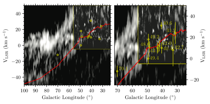
Figure 3: Left panel: Locations (circles with error bar) of the inner Perseus arm sources on a longitude-velocity diagram of CO emission survey (Dame et al., 2001), which is adapted from Figure 8 of Reid et al. (2016), where the Perseus arm in the first Galactic quadrant is traced by the solid line. Within the yellow box at upper right, where the arm is most distant and within the solar circle, the Dame et al. survey is replaced by the higher angular resolution CO survey of Jackson et al. (2006). Right panel: Zoom in plot from the left panel with Galactic longitude of each source is labeled and $V_{\rm LSR}$ error bars shown.

We identify masers associated with the inner Perseus arm based on their coincidence in Galactic longitude ($\ell$) and $V_{\rm LSR}$ ($v$) with a large lane of emission at low absolute velocities that marks the Perseus arm in CO and HI ($\ell-v$) diagrams. As shown in Figure 3, $\ell-v$ loci of all the sources listed in Table 1 are consistent with the trace of the Perseus arm, except for G040.62$-$00.13, whose velocity is about 15 km s^-1 larger than that of other nearby sources, but whose parallax indicates a Perseus arm association. Table 1 lists parallaxes (distances), proper motions and $V_{\rm LSR}$ of all new masers sources reported in this paper together with two sources from Zhang et al. (2013) in the inner Perseus arm. As recently highlighted for Gaia results by Bailer-Jones (2015), estimating distance by simply inverting parallax can result in bias. For a Gaussian parallax, $\Pi$, distribution, the inverse distribution is asymmetric with a peak at $1/\Pi$ and a tail toward larger distances. Thus, the expectation (mean) distance is greater than that of the peak. Therefore, in Table 1, we present two estimates of distance: 1) $1/\Pi$ with asymmetric uncertainties obtained by adding and subtracting the $1\sigma$ parallax uncertainty, and 2) that following Bailer-Jones, with a prior of an exponentially decreasing space density with a length scale of $L=6$ kpc (which implies a mode of 12 kpc for the prior). The differences between distance estimates for any given source are small, since most uncertainties are smaller than $\pm 25$% of the parallax and distances are comparable to the mode of the prior in the Bailer-Jones approach, and we adopt the simpler method 1) values.

Figure 2 shows the locations of HMSFRs determined by trigonometric parallaxes. Table 2 lists the peculiar motions of the HMSFRs, caculated using the Galactic parameters ($R_{0}$ = 8.31 kpc, $\Theta_{0}$ = 241 km s^-1) and the Solar Motion values ($U_{\odot}$ = 10.5 km s^-1, $V_{\odot}$ = 14.4 km s^-1, and $W_{\odot}$ = 8.8 km s^-1), and assuming the universal rotation curve with three parameters $a_{1}$ = 241 km s^-1, $a_{2}$ = 0.90 and $a_{3}$ = 1.46 from Reid et al. (2014).

Combining the eight sources presented here with two sources reported in Zhang et al. (2013), there are now ten sources tracing the inner Perseus arm. As shown in Figure 2, these sources are consistent with following a spiral from Galactic azimuth $\approx$ 50 ^∘ to 110^∘ (corresponding to Galactic longitude $\ell\approx$ 70 ^∘ to 30^∘) and extending nearly 5 kpc in length. Using a Bayesian fitting approach that takes into account uncertainties in distance that map into both $R$ and $\beta$ (Reid et al., 2014) and is insensitive to outliers (Sivia & Skilling, 2006, see “conservative formulation”), we estimate a pitch angle of 5^∘  $\pm$ 4^∘ for the inner portion of the Perseus arm. This is consistent with our previous estimates of 9^∘ $\pm$ 2^∘and 9^∘  $\pm$ 1^∘ determined from the sources confined to the outer and all portions of the Perseus arm (Zhang et al., 2013; Reid et al., 2014), respectively.

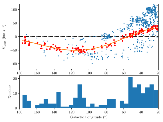
Figure 4: Upper panel: Distribution of WISE HII regions along the Perseus arm in the range of $\ell$ of 20–180^∘, where the HII regions are from the catalog on http://astro.phys.wvu.edu/wise/(see also Anderson et al. 2018). The red dots denote the HII regions which can be assigned to the Perseus arm, which is traced by the solid curve of $\ell-v$ diagram as shown in Figure 8 of Reid et al. (2016); blue dots are sources in other spiral arms. Lower panel: Numbers of WISE HII regions on the Perseus arm versus Galactic longitude.

In our first paper on the inner Perseus arm (Zhang et al., 2013), we suggested the existence of a gap in the distribution of high mass star-forming regions in the Perseus arm based on the lack of masers and the paucity of massive young stellar objects in the Red MSX Source survey (Urquhart et al., 2014). While both suggest a low level of active star formation, the overall small number of 1.1-mm wavelength continuum sources detected in the Bolocam Galactic Plane Survey shows that this part of the Perseus arm is also lacking dense molecular cloud cores, the raw material of present and future star formation (Ginsburg et al., 2013). It is clear from Figure 16 of their study (see also Figure 6 of Shirley et al., 2013) and in the Bolocam source catalog , these authors only found a small number of compact mm-wavelength sources in longitudes between 50^∘ and 80^∘; i.e., a few tens as opposed to many hundreds in longitude ranges of comparable width elsewhere in the plane. In particular, many dense cores are found in the 30^∘ $<\ell<$ 50^∘ range, in which the masers studied by us are located. We also note that Koo et al. (2017) have confirmed the gap, based on the clumpy distribution of HII regions detected in infrared emission with the Wide-Field Infrared Survey Explorer (WISE) catalogued by Anderson et al. (2014). Furthermore, the recently updated HII region catalogue of Anderson et al. (2018) as shown in Figure 4 clearly shows a much lower density of HII regions in 55^∘ $<\ell<$ 100^∘ than in the 30^∘ $<\ell<$ 55^∘ range. The absence of massive star forming material in the Perseus gap supports theories of spiral arm formation in segments (Julian & Toomre, 1966; Grand et al., 2012; D’Onghia et al., 2013; Baba, 2015), rather than global formation on a galaxy-wide scale as assumed by the classic static density wave theory (Lin & Shu, 1964). However, recently the possibility that reflection of spiral density waves might also produce a segmented view of spiral arm star-formation has been forwarded (Shu, 2016).

Additional evidence for segmental arm formation can be found in maser kinematics. Table 3 lists variance-weighted averages of the peculiar motion components of three segments of the Perseus arm with data from Reid et al. (2014) and this paper. There is a significant difference in $\overline{U_{s}}$ between the inner and outer segments (especially the segment in $\ell$ between 90^∘ and 140^∘). This further supports our finding that the Perseus arm is not a single coherent feature, since the inner and the outer segments are moving apart and may be independent.

5 Summary

We report trigonometric parallax and proper motion measurements of 6.7 GHz CH₃OH masers and 22 GHz H₂O masers from eight HMSFRs using the VLBA observations as part of the BeSSeL Survey. The distances of these HMSFRs combined with their Galactic coordinates, radial velocities, and proper motions, allow us to assign them to the inner Perseus arm. These HMSFRs are clustered between Galactic longitudes from $\approx$ 30^∘ to 50^∘, a range for which other tracers indicated an enhanced level of star-formation activity relative to other sections of the Perseus arm.

Table 1: Parallaxes and Proper Motions of Maser Sources in the Inner Perseus arm

Source	Parallax	Distance	$\mu_{x}$	$\mu_{y}$	$V_{\rm LSR}$	Reference
name	(mas)	(kpc)	(mas yr-1)	(mas yr-1)	(km s-1)
G031.24$-$00.11 (H)	0.076 $\pm$ 0.014	$13.2_{-2.0}^{+3.0}$ ( $13.1^{+3.1}_{-2.1})$	$-$2.80 $\pm$ 0.19	$-$5.54 $\pm$ 0.19	24 $\pm$ 10 (021)	This paper
G032.79+00.19 (H)	0.103 $\pm$ 0.031	$~{}9.7_{-2.2}^{+4.1}$ ( $10.0^{+5.1}_{-2.7})$	$-$2.94 $\pm$ 0.24	$-$6.07 $\pm$ 0.25	08 $\pm$ 15 (014)	This paper
G040.42+00.70 (C)	0.078 $\pm$ 0.013	$12.8_{-1.8}^{+2.6}$ ( $12.8^{+2.7}_{-1.9})$	$-$2.95 $\pm$ 0.09	$-$5.48 $\pm$ 0.10	10 $\pm$ 05 (000)	This paper
G040.62$-$00.13 (C)	0.080 $\pm$ 0.021	$12.5_{-2.6}^{+4.4}$ ( $12.4^{+4.7}_{-2.8})$	$-$2.69 $\pm$ 0.09	$-$5.60 $\pm$ 0.25	31 $\pm$ 05 (033)	This paper
G042.03+00.19 (C)	0.071 $\pm$ 0.012	$14.1_{-2.0}^{+2.9}$ ( $14.0^{+2.9}_{-2.1})$	$-$2.40 $\pm$ 0.09	$-$5.64 $\pm$ 0.11	12 $\pm$ 05 (000)	This paper
G043.16+00.01 (H)	0.090 $\pm$ 0.006	$11.1_{-0.7}^{+0.8}$ ( $11.1^{+0.8}_{-0.7})$	$-$2.48 $\pm$ 0.15	$-$5.27 $\pm$ 0.13	11 $\pm$ 05 (016)	Zhang et al. (2013)
G048.60+00.02 (H)	0.093 $\pm$ 0.005	$10.7_{-0.5}^{+0.6}$ ( $10.8^{+0.6}_{-0.6})$	$-$2.89 $\pm$ 0.13	$-$5.50 $\pm$ 0.13	18 $\pm$ 05 (018)	Zhang et al. (2013)
G049.26+00.31 (C)	0.113 $\pm$ 0.016	$~{}8.8_{-1.1}^{+1.4}$ ( $~{}8.9^{+1.6}_{-1.2})$	$-$2.73 $\pm$ 0.15	$-$5.85 $\pm$ 0.19	00 $\pm$ 05 (003)	This paper
G049.41+00.32 (C)	0.132 $\pm$ 0.031	$~{}7.6_{-1.4}^{+2.3}$ ( $~{}7.9^{+3.1}_{-1.8})$	$-$3.15 $\pm$ 0.17	$-$4.49 $\pm$ 0.66	$-$12 $\pm$ 05 (–21)	This paper
G070.18$+$01.74 (C)	0.136 $\pm$ 0.014	$~{}7.3_{-0.7}^{+0.8}$ ( $~{}7.4^{+0.9}_{-0.7})$	$-$2.88 $\pm$ 0.15	$-$5.18 $\pm$ 0.18	$-$23 $\pm$ 05 (000)	This paper

Note. — Column 1 lists source names, where H and C in parentheses denote H₂O and CH₃OH maser, respectively. Column 3 lists two estimates of distance: the distance obtained by inverting the parallax and, in parentheses, using the method of Bailer-Jones (2015). Column 4 to 5 give absolute proper motions in the eastward and northward directions. Column 6 gives estimates of the $V_{\rm LSR}$ of the central star; the first values are from § 3 and the values in parentheses are from the nearest BGPS source (Shirley et al., 2013), where empty parentheses indicate no source within 150″ of the maser position.

Table 2: Peculiar Motions of Maser Sources in the Inner Perseus Arm

Source	$U_{s}$	$V_{s}$	$W_{s}$
name	(km s-1)	(km s-1)	(km s-1)
G031.24$-$00.11	–19.5 $\pm$ 10.6	–12.4 $\pm$ 70.8	6.7 $\pm$ 12.7
G032.79+00.19	15.7 $\pm$ 12.7	–66.2 $\pm$ 98.8	1.9 $\pm$ 13.4
G040.42+00.70	–5.2 $\pm$ 05.4	12.2 $\pm$ 60.2	15.6 $\pm$ 06.0
G040.62$-$00.13	–21.5 $\pm$ 10.0	19.2 $\pm$ 94.3	–2.0 $\pm$ 09.8
G042.03+00.19	–11.3 $\pm$ 05.7	44.8 $\pm$ 67.2	–22.1 $\pm$ 08.9
G043.16+00.01 (W49 N)	–20.6 $\pm$ 06.3	–25.1 $\pm$ 14.3	–3.4 $\pm$ 07.8
G048.60+00.02	–7.7 $\pm$ 05.9	3.3 $\pm$ 09.3	7.3 $\pm$ 06.3
G049.26+00.31	11.6 $\pm$ 07.2	–27.7 $\pm$ 26.1	–5.4 $\pm$ 07.2
G049.41+00.32	–19.6 $\pm$ 20.1	–67.8 $\pm$ 34.0	32.8 $\pm$ 15.7
G070.18$+$01.74	10.8 $\pm$ 05.9	0.5 $\pm$ 14.0	–2.2 $\pm$ 05.8

Note. — Columns 1 lists source names, columns 2 to 4 list peculiar motion components, where $U_{s}$, $V_{s}$, $W_{s}$ are directed toward the Galactic Center, in the direction of Galactic rotation and toward the North Galactic Pole (NGP), respectively. The peculiar motions were estimated using the Galactic parameters ($R_{0}$ = 8.31 kpc, $\Theta_{0}$ = 241 km s^-1) and the Solar Motion values ($U_{\odot}$ = 10.5 km s^-1, $V_{\odot}$ = 14.4 km s^-1, and $W_{\odot}$ = 8.8 km s^-1), and assuming the universal rotation curve with three parameters $a_{1}$ = 241 km s^-1, $a_{2}$ = 0.90 and $a_{3}$ = 1.46 from Reid et al. (2014).

Table 3: Averaged Peculiar Motions of Maser Sources in the Inner Perseus Arm

Segment $\ell$	N	$\overline{U_{s}}$	$\overline{V_{s}}$	$\overline{W_{s}}$
∘		(km s-1)	(km s-1)	(km s-1)
30 – 50	9	-8.4 $\pm$ 2.5	-9.7 $\pm$ 8.3	2.6 $\pm$ 2.8
90 – 140	16	14.1 $\pm$ 1.4	-7.6 $\pm$ 1.4	-1.7 $\pm$ 1.3
170 – 245	9	3.5 $\pm$ 1.8	-3.3 $\pm$ 2.0	-1.2 $\pm$ 1.9

Note. — Column 1 lists segments of the Perseus arm with different ranges of Galactic longitude as shown in Figure 2. Column 2 lists the number of values averaged. Columns 3 to 5 list variances weighted average peculiar motion components of $U_{s}$, $V_{s}$ and $W_{s}$ for the arm segments using the data listed in Table 2 and the data caculated from Table 1 in Reid et al. (2014).

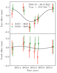
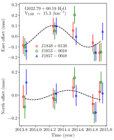
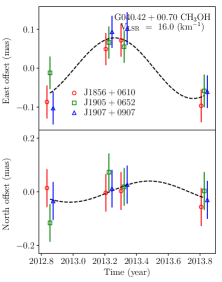
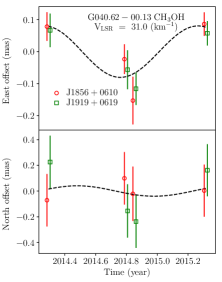
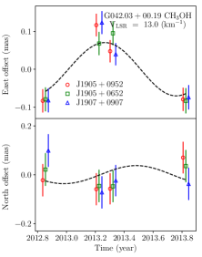
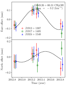
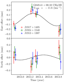
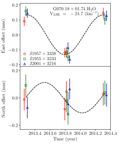
Figure 1: Proper motion-free Parallax signatures. For H₂O masers, the parallax is estimated by combining all the relative position data between the masers and QSOs. For CH₃OH masers, the parallax is estimated using the 1-step method described in § 3. In each panel, for clarity, the data of only one maser spot is plotted. The QSO names used in the data fitting for each source, the $V_{\rm LSR}$ of the maser spot plotted, and the maser source names and its species are labeled.

.

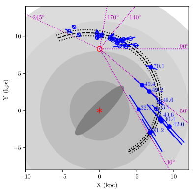
Figure 2: Upper panel: Locations (markers with error bars) of maser sources in the Perseus arm projected on the Galactic plane viewed from the North Galactic Pole. The values of locations are calculated using the trigonometric parallaxes. The filled circles are sources reported in this paper. The Galactic Center (asterisk) is at (0, 0) and the Sun (dot) at (0, 8.31) kpc. The dashed line is a section of the Perseus arm from a weighted fit to the points and corresponds to a global fitted pitch angle of 9^∘, and the dotted lines around the dashed line denotes arm width increasing with Galactocentric radius (Reid et al., 2014). The Galactic longitude of each source is labeled near its location. The dotted straight lines mark select Galactic longitudes discussed in the text.

Table A1: VLBA Observations

Source	Maser	Program	Epochs
Name	Species	Code	(20yymmdd)
G031.24$-$00.11	H2O	BR198L	131104, 140407, 140720, 140914, 141031, 141212, 150417
G032.79+00.19	H2O	BR198O	131106, 140410, 140722, 140920, 141101, 141206
G040.42+00.70	CH3OH	BR149O	121108, 130324, 130428, 131029
G040.62$-$00.13	CH3OH	BR149Q	121117, 130330, 130504, 131030
G042.03+00.19	CH3OH	BR149O	121108, 130324, 130428, 131029
G049.26+00.31	CH3OH	BR149P	121110, 130326, 130429, 131030
G049.41+00.32	CH3OH	BR149Q	121117, 130330, 130504, 131031
G070.18$+$01.74	CH3OH	BR149R	121118, 131026, 131102, 140429

Table A2: Positions and Brightnesses of the Target and Background Sources

Source	R.A. (J2000)	Dec. (J2000)	$\theta_{sep}$	P.A.	$S_{p}$	$V_{\rm LSR}$	Beam
	(h   m   s)	(°   ′   ″)	(°)	(°)	(Jy/beam)	(km s-1)	(mas  mas  °)
G031.24$-$00.11 (21/13)	18 48 45.08390	$-$01 33 13.0980	…	…	9.4	$+$26.0	1.4 $\times$ 0.6 @ 0$-$8
J1857$-$0048	18 57:51.35860	$-$00:48:21.9496	2.4	72	0.011	…	1.5 $\times$ 0.7 @ 0$-$7
J1853$-$0048	18 53:41.98920	$-$00:48:54.3300	1.4	59	0.014	…	1.4 $\times$ 0.6 @ 0$-$10
J1846$-$0003	18 46:03.78500	$-$00:03:38.2800	1.6	–24	0.009	…	1.4 $\times$ 0.7 @ 0$-$8
J1834$-$0301	18 34:14.07460	$-$03:01:19.6270	3.9	–112	0.045	…	1.5 $\times$ 0.6 @ 0$-$8
G032.79+00.19 (8/8)	18:50:30.7408	$-$00:01:59.300	…	…	4.5	$+$15.3	1.4 $\times$ 0.4 @ 0$-$18
J1853$-$0010	18:53:10.2692	$-$00:10:50.740	0.7	102.5	0.005	…	1.9 $\times$ 0.9 @ 0$-$18
J1857$-$0048	18:57:51.35860	$-$00:48:21.9496	2.0	112.8	0.005	…	1.9 $\times$ 0.8 @ 0$-$13
J1848$+$0138	18:48:21.81035	$+$01:38:26.6322	1.8	–17.8	0.014	…	2.1 $\times$ 0.8 @ 0$-$19
G040.42+00.70  (3/1)	19:02:39.6194	+06:59:09.052	…	…	4.6	$+16.0$	5.1 $\times$ 1.7 @ 0$-$21
J1856+0610	18:56:31.8390	+06:10:16.768	1.7	–118	0.065	…	4.6 $\times$ 1.4 @ 0$-$19
J1854+0542	18:54:36.1284	+05:42:59.307	2.4	–122	0.037	…	4.7 $\times$ 1.7 @ 0$-$22
J1907+0907	19:07:41.9634	+09:07:12.397	2.5	30	0.101	…	4.5 $\times$ 1.5 @ 0$-$16
J1905+0652	19:05:21.2105	+06:52:10.780	0.7	100	0.073	…	4.8 $\times$ 1.4 @ 0$-$19
G040.62$-$00.13  (2/2)	19:06:01.62870	+06:46:36.1400	…	…	4.7	+31.0	3.9 $\times$ 2.3 @ 13
J1905+0652	19:05:21.21048	+06:52:10.7803	0.2	–61	0.092	…	7.4 $\times$ 3.5 @ 52
J1856+0610	18:56:31.83880	+06:10:16.7650	2.4	–104	0.186	…	7.7 $\times$ 3.5 @ 50
J1912+0518	19:12:54.25770	+05:18:00.4220	2.3	–131	0.081	…	7.5 $\times$ 3.5 @ 51
J1919+0619	19:19:17.35020	+06:19:42.7700	3.3	98	0.035	…	7.4 $\times$ 3.5 @ 51
G042.03+00.19  (3/3)	19:07:28.1839	+08:10:53.435	…	…	3.1	$+13.0$	5.1 $\times$ 1.6 @ 0$-$20
J1905+0952	19:05:39.8989	+09:52:08.407	1.7	–15	0.090	…	5.7 $\times$ 2.4 @ 0$-$18
J1913+0932	19:13:24.0254	+09:32:45.379	2.0	47	0.019	…	5.6 $\times$ 2.3 @ 0$-$19
J1907+0907	19:07:41.9634	+09:07:12.397	0.9	3	0.118	…	5.7 $\times$ 2.3 @ 0$-$19
J1905+0652	19:05:21.2105	+06:52:10.780	1.4	–158	0.075	…	5.7 $\times$ 2.4 @ 0$-$18
G049.26+00.31  (4/4)	19 20 44.8579	+14 38 26.555	…	…	3.850	–5.0	2.8 $\times$ 1.1 @ 0$-$8
J1913+1307	19 13 14.0063	+13 07 47.343	2.4	–130	0.069	…	4.1 $\times$ 1.5 @ 0$-$19
J1917+1405	19 17 18.0637	+14 05 09.776	1.0	–124	0.060	…	4.0 $\times$ 1.4 @ 0$-$19
J1922+1530	19 22 34.6994	+15 30 10.028	1.0	27	0.061	…	3.5 $\times$ 1.5 @ 0$-$20
J1924+1540	19 24 39.4558	+15 40 43.947	1.4	42	0.357	…	4.0 $\times$ 1.5 @ 0$-$19
G049.41+00.32  (5/5)	19 20 59.1958	+14 46 49.291	…	…	1.160	–11.9	5.8 $\times$ 2.3 @ 0$-$22
J1913+1307	19 13 14.0063	+13 07 47.339	2.5	–131	0.073	…	7.7 $\times$ 3.3 @ 0$-$22
J1917+1405	19 17 18.0638	+14 05 09.774	1.1	–128	0.074	…	7.2 $\times$ 3.0 @ 0$-$25
J1922+1530	19 22 34.6994	+15 30 10.030	0.8	28	0.099	…	7.2 $\times$ 3.0 @ 0$-$25
J1924+1540	19 24 39.4558	+15 40 43.944	1.3	45	0.380	…	7.1 $\times$ 3.2 @ 0$-$22
G070.18$+$01.74  (4/2)	20 00 54.1360	+33 31 31.031	…	…	3.100	–11.9	2.7 $\times$ 1.5 @ 0$+$180
J2001+3323	20 01 42.20694	+33 23 44.7461	0.2	128	0.089	…	2.6 $\times$ 1.4 @ 0$+$177
J1957+3338	19 57 40.54974	+33 38 27.9429	0.7	–80	0.133	…	2.7 $\times$ 1.5 @ 0$+$180
J1955+3233	19 55 56.35092	+32 33 04.5060	1.4	–133	0.031	…	2.7 $\times$ 1.6 @ 0$+$180
J2001+3216	20 01 16.77409	+32 16 46.9435	1.3	176	0.032	…	2.5 $\times$ 1.5 @ 0$+$4

Note. — The fourth and seventh columns give the peak brightnesses ($S_{p}$) and $V_{\rm LSR}$ of reference maser spot. The fifth and sixth columns give the separations ($\theta_{sep})$ and position angles (P.A.) east of north of the background sources relative to the maser. The last column gives the FWHM size and P.A. of the Gaussian restoring beam. All calibrators are from http://astrogeo.org.The two numbers in parentheses after maser source name denote numbers of maser spots with life time longer than 1 yr and used in parallax estimation, respectively.

References

- Anderson et al. (2018) Anderson, L. D., Armentrout, W. P., Luisi, M., et al. 2018, ApJS, 234, 33
- Anderson et al. (2014) Anderson, L. D., Bania, T. M., Balser, D. S., et al. 2014, ApJS, 212, 1
- Baba (2015) Baba, J. 2015, MNRAS, 454, 2954
- Bailer-Jones (2015) Bailer-Jones, C. A. L. 2015, PASP, 127, 994
- Benjamin et al. (2005) Benjamin, R. A., Churchwell, E., Babler, B. L., et al. 2005, ApJ, 630, L149
- Churchwell et al. (2009) Churchwell, E., Babler, B. L., Meade, M. R., et al. 2009, PASP, 121, 213
- Dame et al. (2001) Dame, T. M., Hartmann, D., & Thaddeus, P. 2001, ApJ, 547, 792
- Deller et al. (2007) Deller, A. T., Tingay, S. J., Bailes, M., & West, C. 2007, PASP, 119, 318
- D’Onghia et al. (2013) D’Onghia, E., Vogelsberger, M., & Hernquist, L. 2013, ApJ, 766, 34
- Drimmel (2000) Drimmel, R. 2000, A&A, 358, L13
- Ginsburg et al. (2013) Ginsburg, A., Glenn, J., Rosolowsky, E., et al. 2013, ApJS, 208, 14
- Grand et al. (2012) Grand, R. J. J., Kawata, D., & Cropper, M. 2012, MNRAS, 426, 167
- Gwinn et al. (1992) Gwinn, C. R., Moran, J. M., & Reid, M. J. 1992, ApJ, 393, 149
- Honma (2013) Honma, M. 2013, in Astronomical Society of the Pacific Conference Series, Vol. 476, Astronomical Society of the Pacific Conference Series, ed. R. Kawabe, N. Kuno, & S. Yamamoto, 81
- Jackson et al. (2006) Jackson, J. M., Rathborne, J. M., Shah, R. Y., et al. 2006, ApJS, 163, 145
- Julian & Toomre (1966) Julian, W. H., & Toomre, A. 1966, ApJ, 146, 810
- Kettenis et al. (2006) Kettenis, M., van Langevelde, H. J., Reynolds, C., & Cotton, B. 2006, in Astronomical Society of the Pacific Conference Series, Vol. 351, Astronomical Data Analysis Software and Systems XV, ed. C. Gabriel, C. Arviset, D. Ponz, & S. Enrique, 497
- Koo et al. (2017) Koo, B.-C., Park, G., Kim, W.-T., et al. 2017, PASP, 129, 094102
- Lin & Shu (1964) Lin, C. C., & Shu, F. H. 1964, ApJ, 140, 646
- Ma et al. (1998) Ma, C., Arias, E. F., Eubanks, T. M., et al. 1998, AJ, 116, 516
- Mathewson et al. (1972) Mathewson, D. S., van der Kruit, P. C., & Brouw, W. N. 1972, A&A, 17, 468
- Moscadelli et al. (2010) Moscadelli, L., Xu, Y., & Chen, X. 2010, ApJ, 716, 1356
- Reid et al. (2016) Reid, M. J., Dame, T. M., Menten, K. M., & Brunthaler, A. 2016, ApJ, 823, 77
- Reid & Honma (2014) Reid, M. J., & Honma, M. 2014, ARA&A, 52, 339
- Reid et al. (2009) Reid, M. J., Menten, K. M., Brunthaler, A., et al. 2009, ApJ, 693, 397
- Reid et al. (2014) —. 2014, ApJ, 783, 130
- Reid et al. (2017) Reid, M. J., Brunthaler, A., Menten, K. M., et al. 2017, AJ, 154, 63
- Roberts (1969) Roberts, W. W. 1969, ApJ, 158, 123
- Sanna et al. (2017) Sanna, A., Reid, M. J., Dame, T. M., Menten, K. M., & Brunthaler, A. 2017, Science, 358, 227
- Shirley et al. (2013) Shirley, Y. L., Ellsworth-Bowers, T. P., Svoboda, B., et al. 2013, ApJS, 209, 2
- Shu (2016) Shu, F. H. 2016, ARA&A, 54, 667
- Sivia & Skilling (2006) Sivia, D. S., & Skilling, J. 2006, Data Analysis–A Bayesian Tutorial, 2nd edn. (Oxford Science Publications)
- Urquhart et al. (2014) Urquhart, J. S., Figura, C. C., Moore, T. J. T., et al. 2014, MNRAS, 437, 1791
- van Moorsel et al. (1996) van Moorsel, G., Kemball, A., & Greisen, E. 1996, in Astronomical Society of the Pacific Conference Series, Vol. 101, Astronomical Data Analysis Software and Systems V, ed. G. H. Jacoby & J. Barnes, 37
- Xu et al. (2016) Xu, Y., Reid, M., Dame, T., et al. 2016, Science Advances, 2, e1600878
- Zhang et al. (2013) Zhang, B., Reid, M. J., Menten, K. M., et al. 2013, ApJ, 775, 79