DAMTP-2019-10

Based on Lecture at Royal Society Scientific Discussion Meeting:

Topological Avatars of New Physics, 4-5 March 2019

Keywords: Sphaleron, Topology, Saddle Point, Electroweak Theory

1 Idea of a Sphaleron

A sphaleron is a static, finite-energy solution of classical field equations that is unstable [1]. The origin of the word is from ancient Greek: $\sigma\phi\alpha\lambda\epsilon\rho$o$\varsigma=$ unstable, ready to fall. A sphaleron is a stationary point of the energy, but not a minimum. It is analogous to a transition state in molecular physics – a saddle point in the configuration space of atomic locations. The field theories we consider here are usually Lorentz invariant. Although the sphaleron solution only depends directly on the energy functional for static fields, the way the sphaleron can be produced and decay will depend on the full, time-dependent field equations.

Topological structure in a field theory, together with the scaling properties of the energy, can make a sphaleron’s existence inevitable, although a rigorous proof of this may not be available. Like a topological soliton, a sphaleron is localised in space, and has no translation symmetries, but it sometimes has the maximally allowed rotational symmetry.

Sphalerons can occur in theories without finite-energy solitons, e.g. in the electroweak theory. Sphalerons also occur in theories with solitons, e.g. as monopole-antimonopole pairs [2], and in the Skyrme model.

In a given field theory, let ${\cal C}$ denote the configuration space of static fields satisfying vacuum boundary conditions and having finite energy. ${\cal C}$ is an infinite-dimensional manifold. In gauge theories, we define ${\cal C}$ as the space of fields with gauge transformations quotiented out as far as possible. This can be achieved by judicious gauge fixing.

${\cal C}$ may be connected, or maybe not. In theories with topological solitons, ${\cal C}$ is disconnected. In the simplest and best known cases, the connected components ${\cal C}_{n}$ are labelled by an integer soliton number $n$, called the topological charge. Usually there is a (topological) charge reflection symmetry, so antisolitons with $n$ negative have the same energy as solitons with $n$ positive.

In physical theories, the energy $E$ is bounded below and has a minimum on ${\cal C}$ – the vacuum solution – but it has no maximum. If ${\cal C}$ is disconnected, the vacuum is in ${\cal C}_{0}$, and the energy minimum in ${\cal C}_{1}$ is the stable 1-soliton. Examples of solitons are monopoles and Skyrmions in 3D (three spatial dimensions), vortices, baby Skyrmions and sigma-model lumps in 2D, and kinks in 1D [3, 4]. There are many variants of these types of soliton.

In sectors with higher soliton numbers, $n\geq 2$, it is not so obvious that $E$ attains its minimum. There is a danger that it is energetically favourable for a putative $n$-soliton to break up into clusters with soliton numbers $n-n^{\prime}$ and $n^{\prime}$, for some $n^{\prime}$. If soliton clusters attract, then it is expected that the $n$-soliton exists as a stable, minimal energy solution.

The various possibilities are illustrated by abelian Higgs vortices in 2D, where there is a dimensionless coupling parameter $\lambda$ [5]. For $\lambda<1$ vortices attract and merge, and there is a stable, circularly symmetric $n$-vortex solution for all $n$; for $\lambda>1$ vortices repel, and there is no energy minimum for $n>1$. But the circularly symmetric solution of merged vortices persists as an unstable, static solution of the field equations, i.e. as a sphaleron. It is unstable to break-up into $n$ individual vortices that drift off to infinity. Finally, at critical coupling, $\lambda=1$, there is a whole moduli space of static $n$-vortex solutions, with dimension $2n$. These are all energy minima, having the same energy. The moduli are the $n$ independent vortex locations [6].

2 Morse Theory

Morse theory is a basic tool relating the topology of a manifold $M$ to the stationary points of a function $f$ on $M$ [7]. The theory is simplest for $M$ finite-dimensional, compact, and connected, and with $f$ a function of generic type, meaning that its stationary points are isolated and that the matrix of second derivatives at each stationary point (the Hessian) has only positive and/or negative eigenvalues (and no zero eigenvalues).

For such a function on a two-dimensional, compact, connected surface $M$, there are three types of stationary point: (local) minima, saddle points and (local) maxima, where the Hessian has, respectively, zero, one or two negative eigenvalues. The numbers (denoted $\sharp$) of such stationary points must satisfy the equality

$$\sharp({\rm minima})-\sharp({\rm saddle}\,{\rm points})+\sharp({\rm maxima})$$

$$\qquad=\,{\rm Euler}\,{\rm number}\,{\rm of}\,M\,=\,2(1-{\rm genus})\,,$$ (1)

and there are further (Morse) inequalities that we will not discuss.

For example, on a 2-sphere (genus 0), there may be just 1 minimum and 1 maximum and no saddles, but saddles are inevitable if $\sharp({\rm minima})>1$ or $\sharp({\rm maxima})>1$. As an illustrative function, consider the surface of a cube, which is topologically a sphere. The distance from the centre of the cube is a function of direction, and hence a function on the sphere. It has 6 minima at the face centres, 12 saddles at the edge mid-points, and 8 maxima at the vertices. Note that $6-12+8=2$, as expected. Saddle points are also inevitable for any function on a surface whose genus is greater than 0 (e.g. a torus with genus 1).

On a compact manifold $M$ of any dimension, one can find saddle points of $f$ by connecting a minimum to another minimum by trial paths. Along any such path there will be a point where $f$ has its maximum value, and then one can seek to minimize this maximum value over all paths. The minmax point exists because of the compactness of the surface, and is a saddle of $f$ with one unstable direction. This construction is due to Ljusternik and Schnirelman [8].

The maximum along a single, well-chosen path can give a good estimate for the position of the saddle and an upper bound for the value of $f$ at the saddle.

A variant of this approach works if $f$ has just one minimum, but there are non-contractible loops on $M$, starting and ending at the minimum. Now one finds the point on each loop where $f$ has its maximum, and applies a minmax search to all loops in a particular topological class (homotopy class) of non-contractible loops. This works, e.g. on a torus, and determines a saddle point of $f$.

3 Saddle Points in Field Theory

The method of non-contractible loops can be applied to field theories. Let us assume the minimum of the energy $E$ is unique. The minmax field configuration on a class of loops through the minimum is a saddle point of $E$, i.e. a sphaleron with one unstable mode. Higher-dimensional, non-contractible spheres of fields can be used to find higher-energy saddles with more unstable modes.

This method is not foolproof, because field configuration space is infinite-dimensional and lacks an obvious notion of compactness. Field energy can drift off to infinity in various ways [2]. In particular, the method fails when non-contractible loops exist but spatial rescaling of the fields can reduce the minmax energy to zero. For example, in pure 3D Yang–Mills gauge theory, and 1D sigma models, there are non-contractible loops related to instantons (topologically non-trivial solutions of the field equations in 4D and 2D, respectively), but the maximum of the energy along such a loop can be made arbitrarily small by a length rescaling.

It is also important, when applying the method in a gauge theory, to avoid the use of a non-contractible loop of gauge transformations, along which the energy is simply constant. Morse theory naïvely fails in gauge theory because the Hessian at a stationary point of the energy has infinitely many zero eigenvalues associated with infinitesimal gauge transformations. To avoid this degeneracy it is necessary to fix the gauge.

4 Saddle Points in Gauge/Higgs Theory

In gauge theories with Higgs symmetry breaking one can overcome these difficulties. In a 3D gauge theory with Higgs field $\Phi$, the energy is of the generic form

$$E=\int_{\hbox{\upright\hbox to0.0pt{I\hss}\kern 1.7ptR}^{3}}\left(|F^{2}|+|D\Phi|^{2}+V(|\Phi|)\right)\,d^{3}x\,,$$ (2)

where $F$ is the field tensor constructed from the gauge potential $A$, and $D\Phi$ is the gauge-covariant derivative of $\Phi$. Terms scale in opposite ways under a length rescaling ${\bf x}\to\mu{\bf x}$, so an energy minimum occurs at a finite length scale.

An effective gauge fixing is to impose the radial gauge condition on the gauge potential, $A_{r}=0$. This can be done continuously for any continuous family of gauge and Higgs fields. It depends on choosing an origin, but that is not a problem for energetically localised field configurations.

Superficially, the radial gauge choice allows further gauge transformations depending only on the angular coordinates, but such gauge transformations would generally be singular (multi-valued) at the origin. The only remaining gauge freedom is by rigid (global) gauge transformations. Such global gauge transformations can also be partially suppressed by a base point condition – for example, requiring the Higgs field to take a specified value as one moves off to infinity in a particular direction. Any residual global gauge freedom is usually easy to deal with in the topological discussion.

In the following, we restrict our attention to two well-known examples of gauge/Higgs theory. The first is the Georgi–Glashow model, with gauge group SU(2) and a real, adjoint (triplet) Higgs field $\Phi$ [9]. The standard quartic Higgs potential requires that the vacuum Higgs field lies on the 2-sphere $|\Phi|=1$. The Higgs vacuum manifold is therefore $S^{2}$. The second is the bosonic truncation of the electroweak theory of Weinberg and Salam. Here the gauge group is U(2), with the SU(2) and U(1) coupling constants having independent values (their ratio defines the weak mixing angle). The Higgs field is a complex doublet $\phi$, and again the quartic Higgs potential requires the vacuum Higgs field to satisfy $|\phi|=1$. The Higgs vacuum manifold is therefore $S^{3}$. (Here we have normalised the Higgs fields to absorb the vacuum expectation values. Note that the Higgs vacuum manifold is not a point, because we have fixed the gauge using the gauge potential, and not the Higgs field.)

Finite-energy field configurations have a Higgs field that at spatial infinity takes values on the Higgs vacuum manifold. By imposing the radial gauge condition, $A_{r}=0$, we ensure that the value of the Higgs field on the sphere at infinity is well defined (because the finite-energy condition requires the radial covariant derivative of the Higgs field to decay rapidly). A field configuration is therefore characterised by a mapping from the sphere at infinity to the Higgs vacuum manifold, i.e. by a map $\Phi_{\infty}:S^{2}\to S^{2}$ in the Georgi–Glashow model, and by a map $\phi_{\infty}:S^{2}\to S^{3}$ in the electroweak theory. These maps are well defined up to a global gauge transformation that acts by a global rotation on the target.

There is no further topological information in a field configuration, because in both models the Higgs field is linear and not subject to any constraint. The gauge potential in also essentially linear, so unconstrained in finite regions of space. The gauge potential and Higgs field are correlated at infinity (because angular covariant derivatives of the Higgs field vanish at infinity), but all the topological information about a field configuration, and more importantly, about any continuous family of field configurations, is captured by the family of maps from $S^{2}$ to the Higgs vacuum manifold ($S^{2}$ or $S^{3}$ in our examples).

In the Georgi–Glashow model, the space of these maps is disconnected. A map $\Phi_{\infty}:S^{2}\to S^{2}$ has a degree $n$, and the components of the field configuration space are denoted ${\cal C}_{n}$. Physically, $n$ is the monopole number. This is because, in ${\cal C}_{n}$, the asympototic gauge field has the character of a magnetic monopole field, with magnetic charge proportional to $n$. The minimum of the energy in ${\cal C}_{0}$ is the vacuum, and in the sector ${\cal C}_{1}$ it is the ’t Hooft–Polyakov monopole, which is spherically symmetric [10, 11]. Multi-monopole solutions in the higher sectors ${\cal C}_{n}$ are harder to find; however, they are understood rather well in the limiting version of the theory where the Higgs potential $V$ vanishes, but the asymptotic Higgs field still has a non-zero vacuum expectation value. In this limit, multi-monopole solutions can be found by solving first-order Bogomolny equations [12, 13]. As for vortices at critical coupling, there is a large moduli space of solutions (of dimension $4n$) representing monopoles at arbitrary locations [14]. The location of each monopole accounts for three of the four moduli per monopole. The fourth is a phase that (for one monopole) appears to be a gauge artifact, but it is now well understood that relative phases between monopoles are physical, and even for one monopole, a time-dependent phase is what can give the monopole an electric charge, turning the monopole into a dyon. (Note, the moduli are not simply positions and phases when the monopoles are close together and merge, but the moduli space remains smooth.)

When the Higgs potential $V$ is positive, and the Higgs field massive, there are no Bogomolny equations, so it is necessary to solve the full second-order field equations. Fewer solutions are known in this case, but the basic monopole and the analogue of the most compact of the Bogomolny multi-monopole solutions persist. In particular, a 2-monopole with toroidal symmetry persists [15]. However, the basic monopoles tend to repel each other, making this 2-monopole unstable. It is therefore a sphaleron.

The most interesting sphaleron involving monopoles was proved to exist by Taubes [2]. Taubes considered monopole-antimonopole configurations in the vacuum sector ${\cal C}_{0}$ of the Georgi–Glashow model. Such a pair usually annihilate, but because a monopole has a phase, it is possible to construct a closed loop of monopole-antimonopole configurations where the relative phase increases by $2\pi$. When the relative phase is $0$ or $2\pi$, or indeed any value other than $\pi$, the configuration can simply collapse to the vacuum, but when the phase is $\pi$ the monopole and antimonopole are in an unstable balance. The minmax point along loops of this type is a sphaleron solution, and is unstable to a change of phase away from $\pi$, in either direction. It can be interpreted as a slightly distorted monopole-antimonopole pair at finite separation. The detailed (axisymmetric) solution has been found by careful numerical work [16, 17, 18]. The energy is confirmed to be less than that of a monopole and antimonopole at infinite separation, as anticipated by Taubes’ general reasoning; the magnetic dipole moment has also been calculated.

Taubes’ original argument for the existence of the monopole-antimonopole sphaleron was mainly topological, although combined with careful analysis. The sector ${\cal C}_{0}$ is topologically the space of maps $\Phi_{\infty}:S^{2}\to S^{2}$ with degree 0. This space has non-contractible loops because its first homotopy group is

$$\Pi_{1}({\rm Maps}(S^{2}\to S^{2}))=\Pi_{3}(S^{2})=\hbox{\upright\hbox to0.0pt{\sans Z\hss}\kern 2.7pt{\sans Z}}\,,$$ (3)

where $\Pi_{3}(S^{2})$ denotes the third homotopy group of $S^{2}$. This result is a special case of a very useful, more general result for based maps,

$$\Pi_{k}({\rm Maps}(S^{l}\to M))=\Pi_{k+l}(M)\,.$$ (4)

Taubes’ work on the monopole-antimonopole solution was the inspiration behind the discovery by this author, in collaboration with F. Klinkhamer, of the electroweak sphaleron [19, 1]. In the electroweak theory, the asymptotic Higgs field (in radial gauge) defines a map $\phi_{\infty}:S^{2}\to S^{3}$. The space of such maps is connected, so the field configuration space ${\cal C}$ has just one component. From a topological perspective, therefore, there are no topological soliton charges in the electroweak theory, and in particular, no smooth, finite-energy monopole solutions are expected.

However, ${\cal C}$ has non-contractible loops, because

$$\Pi_{1}({\rm Maps}(S^{2}\to S^{3}))=\Pi_{3}(S^{3})=\hbox{\upright\hbox to0.0pt{\sans Z\hss}\kern 2.7pt{\sans Z}}\,.$$ (5)

By applying the minmax argument to such loops, and by more detailed work constructing fields and solving the field equations, it was possible to find an explicit sphaleron solution in the electroweak theory. Higher-energy sphalerons with more unstable modes have also been found, by considering non-contractible spheres of electroweak fields [20].

5 Properties of the Electroweak Sphaleron

A limiting version of electroweak theory is where the weak mixing angle vanishes. This is the limit where the U(1) field decouples and the masses of the $W$ and $Z$ bosons are equal. The field equations reduce to those of an SU(2) gauge field coupled to a complex Higgs doublet, and the sphaleron is spherically symmetric in this case. The version of electroweak theory that is realised in nature is not far from this limit. The observed weak mixing angle is less than $30^{\circ}$ and the $Z$ boson mass is about 91 GeV, not much larger than 80 GeV, the mass of the $W$ bosons. In the full U(2) electroweak theory the sphaleron is axisymmetric, and has a magnetic dipole moment [1, 21]. Recall that the unbroken gauge group is the electromagnetic U(1), so the long-range field of a static solution is purely magnetic.

The energy of the sphaleron depends on the Higgs boson mass and on the weak mixing angle. When the sphaleron solution was originally discovered, the Higgs boson had not been observed, and its mass was poorly constrained. The sphaleron energy was then estimated to be somewhere in the range 8 – 14 TeV. Now that the Higgs boson is known to have a mass of 125 GeV, a little more than the mass of the $Z$ boson, the sphaleron energy is estimated to be approximately 9 TeV. This assumes that one can rely purely on the classical field equations, combined with the experimentally determined coupling and mass parameters. The contribution of the magnetic dipole field to the energy is only about $1\%$.

A Higgs boson mass of 125 GeV is rather small from one perspective. The sphaleron solution for this mass has $\phi=0$ at its centre, but it has been shown that for very large Higgs mass, of order 1 TeV or higher, the sphaleron solution has a broken discrete symmetry, and the field value $\phi=0$ is not attained at any point in space [22, 23]. The solution is closer to $|\phi|=1$ everywhere, and in the limit of infinite Higgs boson mass, the electroweak sphaleron becomes a gauged Skyrmion [24]. This exists in an effective field theory where the Higgs field is constrained to its vacuum manifold $S^{3}$, changing the topology of the theory, but the relatively recent observation of the Higgs boson rules this effective field theory out.

The sphaleron energy density is remarkably high. The length scale of the solution is the inverse of the masses of the contributing gauge and Higgs fields, of order $(100\,{\rm GeV})^{-1}$. This is approximately $10^{-17}$ m, about 100 times smaller than the length scale of a proton. The sphaleron volume is therefore about $10^{6}$ times smaller than that of a proton. As the sphaleron energy is about $10^{4}$ times the mass of a proton, its energy density is about $10^{10}$ times that of a proton at rest. This, by itself, suggests the sphaleron is hard to produce.

Such energy densities appear to be unreachable in collisions at the LHC – CERN’s Large Hadron Collider. There, colliding protons each have an energy of more than 6 TeV (let’s optimistically call this 10 TeV) and they are Lorentz contracted in the centre of mass frame by a factor of $10^{4}$, the ratio of 10 TeV to the proton mass of 1 GeV. The energy density is therefore $10^{8}$ times that of a proton at rest, and it is in the form of a rather thin pancake, as there is no transverse Lorentz contraction. This does not appear to be enough to produce sphalerons, although there are millions of collisions per second, and large fluctuations of the energy density must sometimes occur. Even if the energy density were two orders of magnitude larger, it could be hard to produce a sphaleron as the field energy, mainly in the form of quarks and gluons, would have to transfer into a coherent combination of $W$, $Z$ and Higgs fields. Such a field can be interpreted as a coherent combination of about 10 each of $W^{\pm}$, $Z$ and Higgs particles. Therefore, the non-perturbative process of sphaleron production in particle collisions is generally thought to be exponentially suppressed, in the same way that soliton-antisoliton production is suppressed [25]. However, the production rate may be enhanced if a strong magnetic field is present, in a region comparable to the sphaleron size. And the production rate is almost certainly enhanced at high temperatures [26].

Whether production of a sphaleron in particle collisions is at all likely may become clearer when experiments at LHC, or at somewhat higher energy, find evidence for simultaneous production of two or more Higgs particles together with a few $W$ or $Z$ bosons. The signal for this would be the production of several high-energy leptons (electrons, muons or neutrinos).

Remarkably, sphaleron production and decay is associated with a net change in baryon number $B$ and lepton number $L$ [27]. This is the result of an anomaly in baryon and lepton number conservation laws, and related to the fact that a sphaleron has Chern–Simons number $\frac{1}{2}$. Sphaleron production is therefore potentially extremely important, as it may help us understand the baryon asymmetry of the universe. The universe is dominated by matter (protons) rather than antimatter (antiprotons) but the source of the asymmetry remains unknown (although there are many ideas). Certainly, any observation of baryon or lepton number violation would be revolutionary, as no experiment so far has ever detected such a violation. However, measuring a net change in baryon number in a high-energy collision may be hard, as many mesons and baryons, and also antibaryons, are produced. It may be easier to keep track of charged leptons, but the neutrinos carry lepton number too, and are generally undetected.

6 Sphalerons in the Skyrme model

The Skyrme model is a field theory of mesons, an effective theory of the strong interactions at relatively low energy, in which the quarks and gluons of QCD have been eliminated [28, 3, 29]. It has topological solitons – Skyrmions – that provide models for nucleons (protons and neutrons) and all larger atomic nuclei.

The basic Skyrme model just has interacting pion fields, the three pion particles being the lightest mesons, but variants have additional fields representing rho and/or omega mesons. In detail, the Skyrme model is a 3D sigma model, meaning that its field $U({\bf x})$, at a given time, is a map from $\hbox{\upright\hbox to0.0pt{I\hss}\kern 1.7ptR}^{3}$ to a target space SU(2). An SU(2) matrix $U({\bf x})$ can be written as

$$U({\bf x})=\sigma({\bf x})1_{2}+i(\pi_{1}({\bf x})\tau_{1}+\pi_{2}({\bf x})\tau_{2}+\pi_{3}({\bf x})\tau_{3})\,,$$ (6)

where $\tau_{i}$ are the three Pauli matrices, and the constraint $\sigma^{2}+\pi_{1}^{2}+\pi_{2}^{2}+\pi_{3}^{2}=1$ needs to be imposed. This links the Skyrme field $U$ with pion fields $\pi_{1},\pi_{2},\pi_{3}$ and explains the name ‘sigma model’. The energy of a (static) Skyrme field is an integral of terms mainly involving the gradient of $U$, with an additional term proportional to $1-\sigma({\bf x})$ that accounts for the small mass of pions.

The group SU(2), regarded as a manifold, is the 3-sphere $S^{3}$, as is implied by the above constraint. For the energy of a Skyrme field to be finite, the boundary condition $U\to 1_{2}$ as $|{\bf x}|\to\infty$ must be satisfied. This boundary condition allows a topological compactification of space to a 3-sphere, by adding a point at infinity. A Skyrme field therefore becomes a based map $U:S^{3}\to S^{3}$ (the base point condition being that the point at infinity maps to the unit element of SU(2)).

A map $U:S^{3}\to S^{3}$ is characterised topologically by its degree, an integer $B$. The configuration space of the Skyrme model is therefore disconnected, with its component ${\cal C}_{B}$ being the sector with baryon number $B$. The notation $B$ rather than $n$ is used, as $B$ is identified with baryon number. This was Skyrme’s great insight – that a nonlinear theory of interacting pions could also account for baryons, by treating baryon number as topological.

In any continuous field evolution, the baryon number does not change in the basic Skyrme model. However, when the Skyrme model is extended to include electroweak fields then the topological structure is more complicated, and the baryon number and lepton number violation induced by electroweak sphalerons that we discussed in the last section are probably possible. I’m not sure if the details of this have been worked out, but a related phenomenon in the context of Skyrmions is the expectation of baryon and lepton number violation when Skyrmions interact with monopoles [30].

The various components ${\cal C}_{B}$ of the Skyrme model have been much studied. For many values of $B$, the minimal energy solution has been found, and is known as the Skyrmion with baryon number $B$. Finding this requires considerable numerical work, but various analytical and geometric ideas have been helpful to set up initial configurations close to true solutions. It appears that in the basic Skyrme model, the global minimum of the energy is attained in each sector ${\cal C}_{B}$, but there is no proof of this. Calculations suggest that it is not favourable for a Skyrme field of baryon number $B$ to break up into infinitely-separated subclusters whose baryon numbers add up to $B$, but these calculations have loopholes [31, 32].

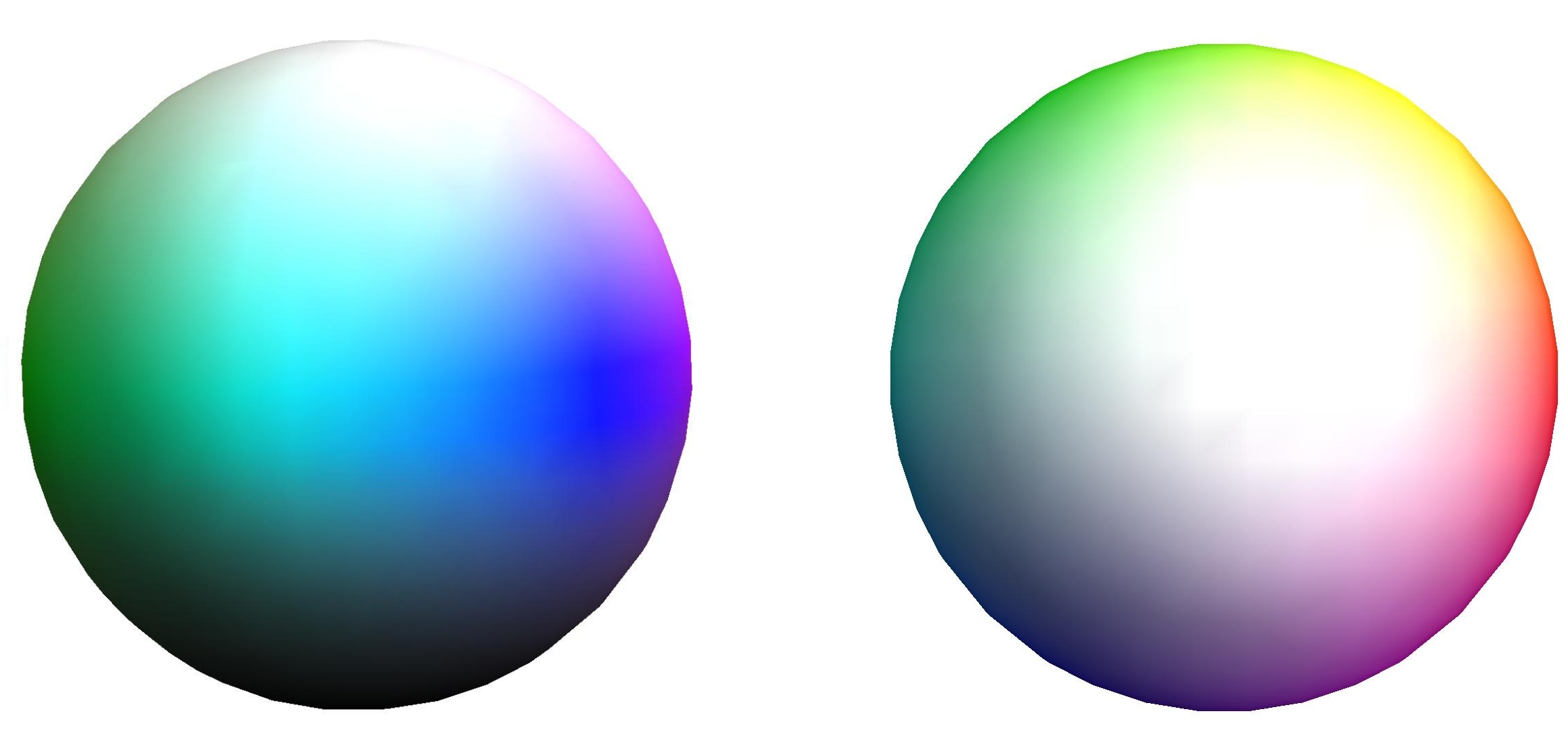
Figure 1: $B=1$ Skyrmion (two different orientations)

The known Skyrmions with baryon numbers $B=1,2,3$ and $4$ have, respectively, spherical, toroidal, tetrahedral and cubic symmetries [33]. The solutions with $B=1$ and $B=4$ are shown in Figs. 1 and 2. A surface of constant energy density is displayed, and the colouring indicates which pion fields have dominant values close to $1$ or $-1$. The coupling parameters of the Skyrme model are chosen so that the $B=1$ Skyrmion has an energy scale and length scale comparable to those of a nucleon. However the classical Skyrmion by itself does not model such a particle. For this it is necessary to quantize the rotational motion of the Skyrmion to obtain spin $\frac{1}{2}$ states [34]. The possibility of spin $\frac{1}{2}$ arises from topology. The relevant space of maps has a non-trivial first homotopy group

$$\Pi_{1}({\rm Maps}(S^{3}\to S^{3}))=\Pi_{4}(S^{3})=\hbox{\upright\hbox to0.0pt{\sans Z\hss}\kern 2.7pt{\sans Z}}_{2}\,,$$ (7)

so there are non-contractible loops. In particular, it has been shown that a rotation of a $B=1$ Skyrmion by $2\pi$ is such a loop. The quantum theory therefore allows the Skyrmion’s wavefunction to acquire a sign change under the $2\pi$ rotation; the wavefunction is single-valued only on the universal, double cover of the the field configuration space [35]. That is why the quantized $B=1$ Skyrmion can represent a spin $\frac{1}{2}$ proton or neutron. The proton and neutron are distinguished by their isospin state, which arises from the quantized isospin symmetry of the Skyrme model that rotates the three pion fields among themselves.

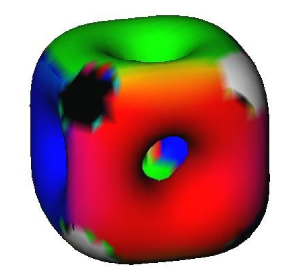
Figure 2: $B=4$ Skyrmion

The topology of the space of maps $U:S^{3}\to S^{3}$ is quite rich, so within each sector ${\cal C}_{B}$ there are non-contractible loops and spheres of various dimensions, and as a result, there are numerous unstable solutions of the field equations, i.e. sphalerons in the Skyrme model. Some of these have quite low energy, only slightly higher than the minimal energy Skyrmion in that sector. It is not possible to describe all solutions of this type systematically, so we just mention a few that are known.

For each positive baryon number, and not just $B=1$, there is a spherically symmetric solution [36]. The field has an angular dependence like the $B=1$ solution, accompanied by a radial profile function that winds $B$ times between the field values $U=1_{2}$ and $U=-1_{2}$. The structure is onion-like, and this is not at all energetically favourable, so apart from the $B=1$ solution, all these solutions are unstable. For example, in the limit of massless pions, the spherically symmetric $B=2$ solution has energy 2.98 times that of the $B=1$ solution, and has six unstable modes, whereas the toroidal $B=2$ solution has energy 1.91 times that of the $B=1$ solution, and is stable.

There was an attempt to use the unstable manifold of the spherically symmetric solution (defined by following the curves of steepest descent of the energy) as a landscape of $B=2$ field configurations, but there are technical and numerical difficulties with this [37, 38]. To connect the Skyrme model with nuclear physics, it is desirable to find finite-dimensional configuration spaces of Skyrme fields to quantize, for each $B$. Rigid-body quantization of Skyrmions (the stable minima of the Skyrme energy) is the best known approach to quantization [34], but imposes too strong constraints on the dynamics. States of nuclei do not simply form a single band of rotational excitations of one underlying structure. At the very least, vibrations away from the minimal energy Skyrmion should be included [39], and quantized, but to do this in a consistent nonlinear way is not easy. Using the unstable manifolds of saddle point solutions still appears to be an attractive route towards a systematic approach to quantization.

There is a large class of unstable, sphaleron solutions in the vacuum sector of the Skyrme model, with $B=0$. Some of these are Skyrmion-antiSkyrmion configurations in unstable equilibrium [40, 41], analogous to the monopole-antimonopole solution of Taubes. An alternative construction is to select an equatorial 2-sphere of the target $S^{3}$, and seek solutions whose values lie everywhere in this 2-sphere. The Skyrme model with target restricted to $S^{2}$ is the Skyrme–Faddeev model, known to have many solutions with a knot-like character, called Hopfions. These solutions may have some interpretation within the purely mesonic or gluonic sector of strong interactions, for example as glueballs, but further investigation of their role is needed. All these solutions are unstable within the Skyrme model, as the target $S^{2}$ can be slipped off the equator of $S^{3}$, making it smaller and reducing the field energy [42].

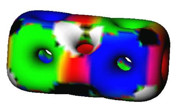
Figure 3: $B=8$ Skyrmion

For higher $B$, above about $B=7$, it is found that the landscape of local minima in the Skyrme model becomes quite complicated, and it is hard to determine numerically which of the local minima is the global minimum. The energies of these minima are very close, and it doesn’t really matter which is the global minimum (the true Skyrmion), as a successful quantization should incorporate all the fields with energy close to the minimum. Between these local minima there are inevitably saddle point solutions, and some of these have energies only a little higher than the local minima.

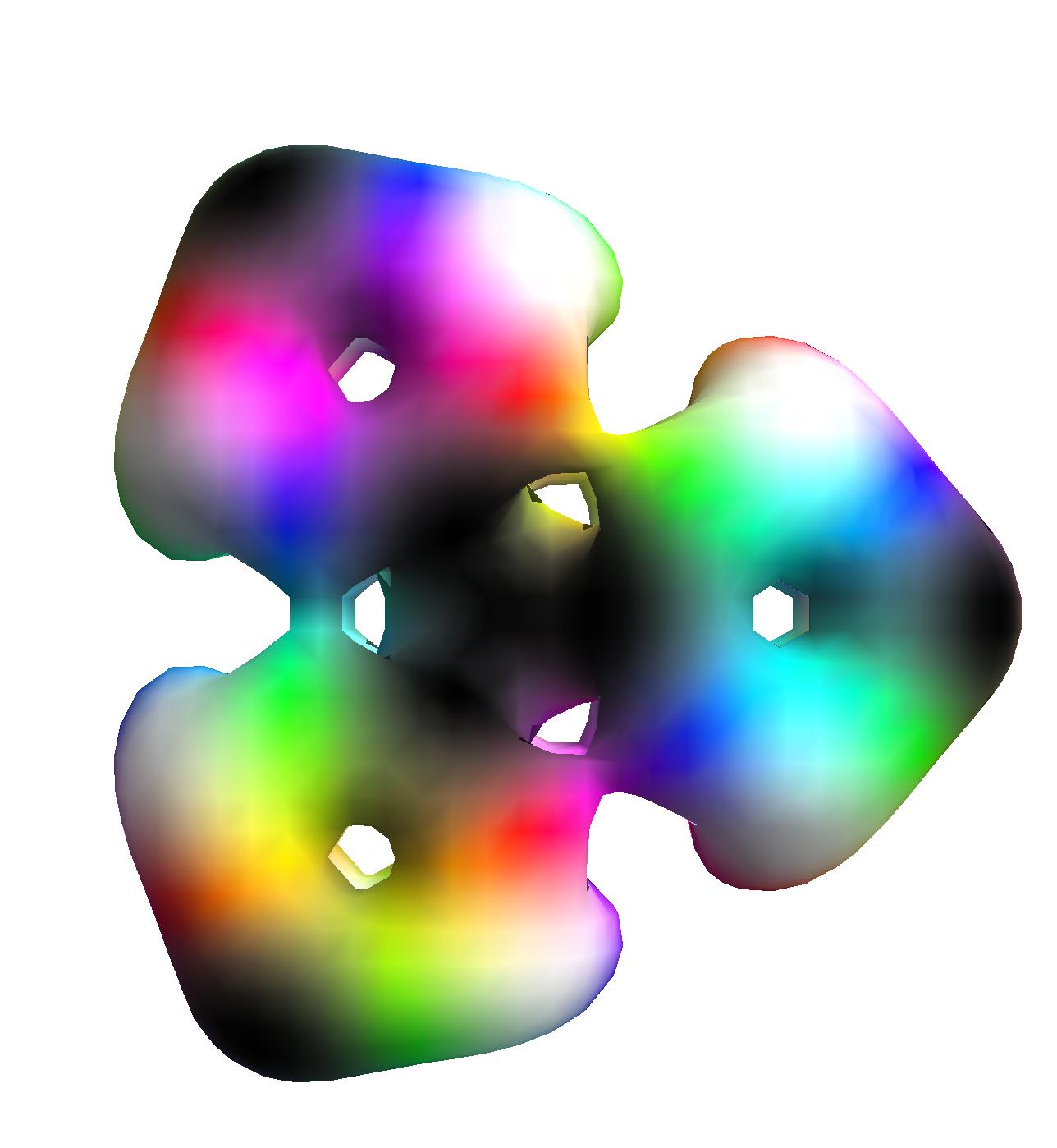
Figure 4: $B=12$ Skyrmion with $D_{3h}$ symmetry

An example occurs for $B=8$ [43, 44]. One solution is shown in Fig. 3 and this is the global minimum of the energy when the pion mass is close to its physical value. Its rigid-body quantization gives a reasonable model for the Beryllium-8 nucleus, but is less successful for the isobars Lithium-8 and Boron-8 [45]. The solution is clearly made of two $B=4$ cubic Skyrmions brought close together. In the $B=8$ solution, the merged faces of the cubes have the same colour (red in the figure), because this is what leads to an attraction. However, it is still possible to twist one cube relative to the other around the line joining them, and this takes little energy. So there is a solution similar to that in Fig. 3 where the two cubes have the same orientation (both nearby faces are green or blue, rather than one green and one blue), but this is slightly unstable to untwisting [39]. Rotating one cube relative to the other by $\pi$ creates a closed loop of field configurations along which there is one minimum of the energy and one saddle point. A good quantization should take into account the degree of freedom along the loop, in addition to all the rigid-body degrees of freedom (translations, rotations, isospin rotations). This would give a better model of Beryllium-8 and its isobars than simply rigid-body quantization.

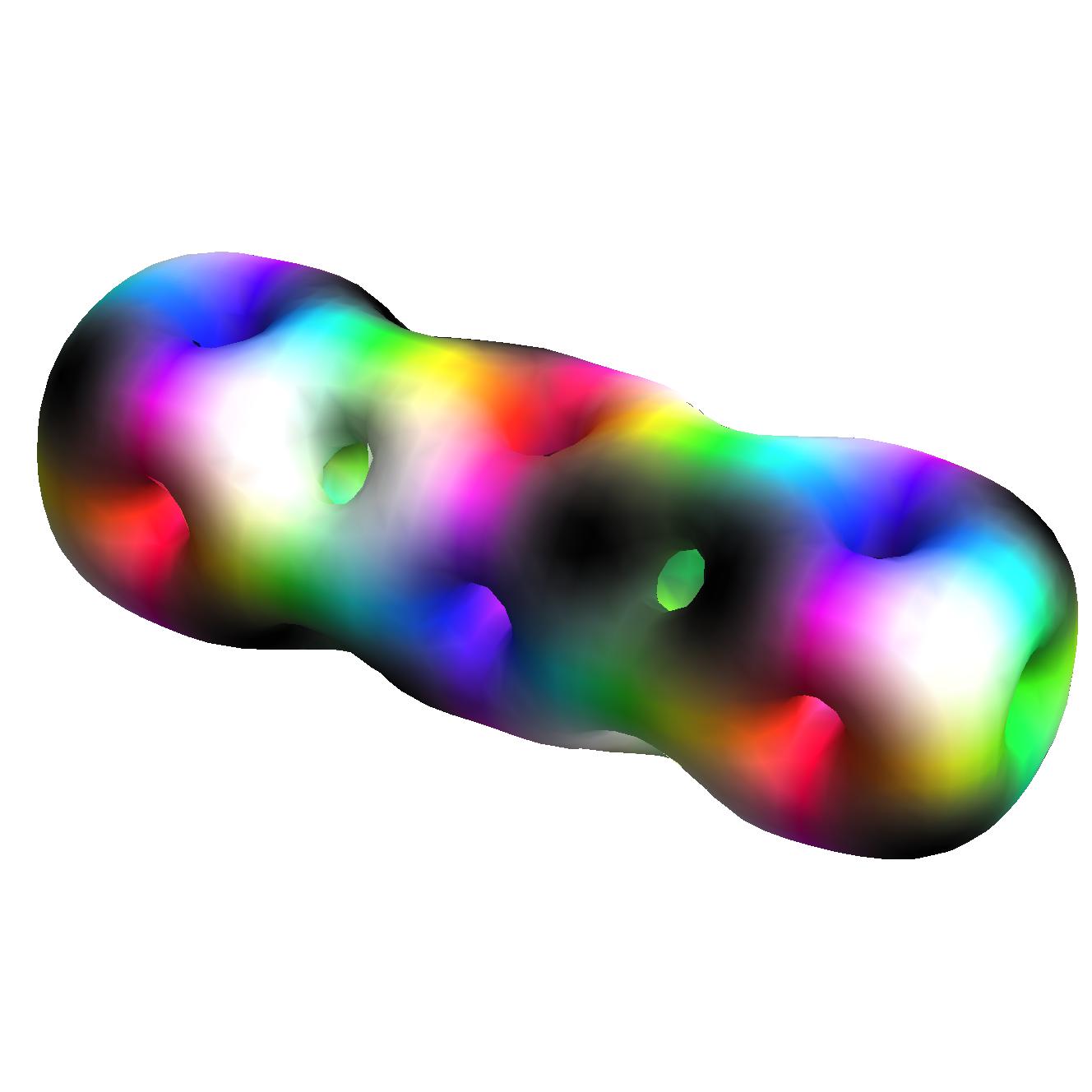
Figure 5: $B=12$ Skyrmion with $D_{4h}$ symmetry

As a final example, we show two solutions with $B=12$ in Figs. 4 and 5 [43, 46]. These consist of three $B=4$ cubes arranged to attract, forming an equilateral triangle or a straight chain. Again their energies are very similar, and it is not clear which is the true Skyrmion. It is possible that one shape is stable and the other is a saddle point, but it is also possible for both to be local minima, with a saddle point (of L-shape) in between. These different scenarios are hard to distinguish, and are sensitive to the exact value of the pion mass, and which variant of the Skyrme model one works with. Quantization of these configurations separately (treating them as well separated by an energy barrier) has given a moderately good understanding of the ground and excited states of Carbon-12 [47], including the Hoyle state, but a better model is obtained by taking account of the landscape between these configurations [48].

7 Conclusions

Unstable, saddle points of the energy occur frequently in field theory – they are called sphaleron solutions, in contrast to the stable solitons that may also exist. Sphalerons often have a topological interpretation, and are related to non-contractible loops or spheres in field configuration space ${\cal C}$. A saddle point is also expected to occur between any pair of local energy minima in a connected component of ${\cal C}$.

Gauge-Higgs theories in 3D are good sources of sphalerons, as well as solitons, as these theories have nontrivial topology captured by the Higgs field at infinity (in radial gauge) and the solutions have a preferred, finite length scale.

The electroweak sphaleron is one such solution. Its energy of 9 TeV has now been reached in proton collisions at the LHC, but the sphaleron’s very high energy density, and its coherent electroweak field structure make it hard to produce.

There has been an interesting suggestion (discussed at this Royal Society meeting) that it could be easier to create a sphaleron in a strong magnetic field. Some of the strongest known fields arise briefly in heavy ion collisions at the LHC. The effective energy of an electroweak sphaleron will be lower in a strong magnetic field, whenever its magnetic dipole moment is aligned with the field.

References

- [1] F. R. Klinkhamer and N. S. Manton, A saddle-point solution in the Weinberg-Salam theory, Phys. Rev. D30, 2212 (1984).
- [2] C. H. Taubes, The existence of a non-minimal solution to the Yang-Mills-Higgs equations on : Part I, Commun. Math. Phys. 86, 257 (1982); Part II, ibid 86, 299 (1982).
- [3] N. Manton and P. Sutcliffe, Topological Solitons, Cambridge University Press, 2004.
- [4] Y. M. Shnir, Topological and Non-Topological Solitons in Scalar Field Theories, Cambridge University Press, 2018.
- [5] L. Jacobs and C. Rebbi, Interaction energy of superconducting vortices, Phys. Rev. B19, 4486 (1979).
- [6] A. Jaffe and C. Taubes, Vortices and Monopoles, Boston, Birkhäuser, 1980.
- [7] J. Milnor, Morse Theory (Annals of Math. Studies 51), Princeton University Press, 1969.
- [8] L. A. Ljusternik, The Topology of the Calculus of Variations in the Large (Amer. Math. Soc. Transl. 16), Providence, American Mathematical Society, 1966.
- [9] H. Georgi and S. L. Glashow, Unified weak and electromagnetic interactions without neutral currents, Phys. Rev. Lett. 28, 1494 (1972).
- [10] G. ’t Hooft, Magnetic monopoles in unified gauge theories, Nucl. Phys. B79, 276 (1974).
- [11] A. M. Polyakov, Particle spectrum in quantum field theory, JETP Lett. 20, 194 (1974).
- [12] E. B. Bogomolny, The stability of classical solutions, Sov. J. Nucl. Phys. 24, 449 (1976).
- [13] M. F. Atiyah and N. J. Hitchin, The Geometry and Dynamics of Magnetic Monopoles, Princeton University Press, 1988.
- [14] E. J. Weinberg, Parameter counting for multimonopole solutions, Phys. Rev. D20, 936 (1979).
- [15] B. Kleihaus, J. Kunz and D. H. Tchrakian, Interaction energy of ’t Hooft–Polyakov monopoles, Mod. Phys. Lett. A13, 2523 (1998).
- [16] B. Rüber, Eine axialsymmetrische magnetische Dipollösung der Yang-Mills-Higgs-Gleichungen, Diplomarbeit, Universität Bonn, 1985.
- [17] B. Kleihaus and J. Kunz, Monopole-antimonopole solution of the Yang-Mills-Higgs model, Phys. Rev. D61, 025003 (2000).
- [18] A. Saurabh and T. Vachaspati, Monopole-antimonopole interaction potential, Phys. Rev. D96, 103536 (2017).
- [19] N. S. Manton, Topology in the Weinberg-Salam theory, Phys. Rev. D28, 2019 (1983).
- [20] F. R. Klinkhamer, Construction of a new electroweak sphaleron, Nucl. Phys. B410, 343 (1993).
- [21] M. E. R. James, The sphaleron at non-zero Weinberg angle, Z. Phys. C55, 515 (1992).
- [22] J. Kunz and Y. Brihaye, New sphalerons in the Weinberg-Salam theory, Phys. Lett. B216, 353 (1989).
- [23] L. G. Yaffe, Static solutions of -Higgs theory, Phys. Rev. D40, 3463 (1989).
- [24] G. Eilam, D. Klabucar and A. Stern, Skyrmion solutions to the Weinberg-Salam model, Phys. Rev. Lett. 56, 1331 (1986).
- [25] S. V. Demidov and D. G. Levkov, Soliton-antisoliton pair production in particle collisions, Phys. Rev. Lett. 107, 071601 (2011).
- [26] D. Yu. Grigoriev, V. A. Rubakov and M. E. Shaposhnikov, Sphaleron transitions at finite temperatures: Numerical study in (1+1) dimensions, Phys. Lett. B216, 172 (1989); Topological transitions at finite temperatures: A real-time numerical approach, Nucl. Phys. B326, 737 (1989).
- [27] G. ’t Hooft, Symmetry breaking through Bell-Jackiw anomalies, Phys. Rev. Lett. 37, 8 (1976); Computation of the quantum effects due to a four-dimensional pseudoparticle, Phys. Rev. D14, 3432 (1976).
- [28] T. H. R. Skyrme, A non-linear field theory, Proc. R. Soc. Lond. A260, 127 (1961); A unified field theory of mesons and baryons, Nucl. Phys. 31, 556 (1962).
- [29] M. Rho and I. Zahed (eds.), The Multifaceted Skyrmion, 2nd ed., Singapore, World Scientific, 2017.
- [30] M. Chemtob, Cross section of monopole-induced Skyrmion decay, Phys. Rev. D39, 2013 (1989).
- [31] N. S. Manton, B. J. Schroers and M. A. Singer, The interaction energy of well-separated Skyrme solitons, Commun. Math. Phys. 245, 123 (2004).
- [32] B. J. Schroers, On the existence of minima in the Skyrme model, PoS unesp2002 (2002) 034 (Proceedings of Workshop on Integrable Theories, Solitons and Duality, São Paolo, 2002).
- [33] E. Braaten, S. Townsend and L. Carson, Novel structure of static multisoliton solutions in the Skyrme model, Phys. Lett. B235, 147 (1990).
- [34] G. S. Adkins, C. R. Nappi and E. Witten, Static properties of nucleons in the Skyrme model, Nucl. Phys. B228, 552 (1983).
- [35] D. Finkelstein and J. Rubinstein, Connection between spin, statistics and kinks, J. Math. Phys. 9, 1762 (1968).
- [36] A. D. Jackson and M. Rho, Baryons as chiral solitons, Phys. Rev. Lett. 51, 751 (1983).
- [37] N. S. Manton, Unstable manifolds and soliton dynamics, Phys. Rev. Lett. 60, 1916 (1988).
- [38] M. F. Atiyah and N. S. Manton, Geometry and kinematics of two Skyrmions, Commun. Math. Phys. 153, 391 (1993).
- [39] S. B. Gudnason and C. Halcrow, Vibrational modes of Skyrmions, Phys. Rev. D98, 125010 (2018).
- [40] S. Krusch and P. Sutcliffe, Sphalerons in the Skyrme model, J. Phys A: Math. Theor. 37, 9037 (2004).
- [41] Ya. Shnir and D. H. Tchrakian, Skyrmion – anti-Skyrmion chains, J. Phys A: Math. Theor. 43, 025401 (2010).
- [42] D. Foster, The decay of Hopf solitons in the Skyrme model, J. Phys A: Math. Theor. 50, 405401 (2017).
- [43] R. A. Battye, N. S. Manton and P. M. Sutcliffe, Skyrmions and the -particle model of nuclei, Proc. R. Soc. Lond. A463, 261 (2007).
- [44] D. T. J. Feist, Interactions of Skyrmions, JHEP 1202, 100 (2012).
- [45] R. A. Battye, N. S. Manton, P. M. Sutcliffe and S. W. Wood, Light nuclei of even mass number in the Skyrme model, Phys. Rev. C80, 034323 (2009).
- [46] P. H. Lau, Construction and Quantisation of Skyrmions, Cambridge University Ph.D. thesis, 2015.
- [47] P. H. C. Lau and N. S. Manton, States of Carbon-12 in the Skyrme model, Phys. Rev. Lett. 113, 232503 (2014).
- [48] J. I. Rawlinson, An alpha particle model for Carbon-12, Nucl. Phys. A975, 122 (2018).