Visualization and Interpretation of Latent Spaces for Controlling Expressive Speech Synthesis through Audio Analysis

Abstract

The field of Text-to-Speech has experienced huge improvements last years benefiting from deep learning techniques. Producing realistic speech becomes possible now. As a consequence, the research on the control of the expressiveness, allowing to generate speech in different styles or manners, has attracted increasing attention lately. Systems able to control style have been developed and show impressive results. However the control parameters often consist of latent variables and remain complex to interpret.

In this paper, we analyze and compare different latent spaces and obtain an interpretation of their influence on expressive speech. This will enable the possibility to build controllable speech synthesis systems with an understandable behaviour.

Index Terms: expressive speech synthesis, affective computing, deep learning, latent space, style embeddings, supervised, unsupervised

1 Introduction

During the last few years, many Text-to-Speech systems based on Deep Learning were developed and showed remarkable performance in terms of reliability and quality of speech. Lately, researchers in this area have been focusing on controlling the speech variability of this kind of systems [1, 2, 3].

An issue for such a control is the lack of data labeled with information such as emotion or style. Emotion modeling is thus one of the main challenges in developing more natural human-machine interfaces. Two main approaches exist to modeling emotions.

A first representation is the categorical representation, such as Ekman’s six basic emotion model [4] which identify anger, disgust, fear, happiness, sadness and surprise as six basic emotions from which the other emotions may be derived. Some speech datasets [5, 6, 7, 8] are annotated in emotional categories. This kind of datasets allow the development of category based emotional TTS [9, 10]. The disadvantage of such simple annotation is that they do not offer a continuous representation of emotion.

Emotions can also be represented in a multidimensional continuous space like in the Russels circumplex model [11]. This modeling allows to better reflect the complexity and the variations in the expressions, unlike the category system. The two most commonly used dimensions in the literature are the arousal corresponding to the level of excitation and the valence corresponding to the pleasure level or positiveness of the emotion. In datasets [12, 13] annotated in emotional dimensions, for each utterance, the final emotion value were obtained by averaging over all annotated results from raters. However they are not suitable for synthesis purpose because they contain overlapping speech due to the data recording setup (dyadic conversation) and some external noise. Moreover, humans are not reliable for giving absolute values to estimate subjective emotional variables [14].

Some researchers tackled the problem of how to capture emotional representation by training systems on other tasks, leading to different approaches employing transfer learning techniques [15].

Recent researches have proposed unsupervised techniques to achieve controllable speech synthesis, avoiding the problem of labels.

In [16], the authors present an extension to the Tacotron speech synthesis architecture that learns a latent embedding space by encoding audio into a vector that conditions Tacotron along with the text representation. These latent embeddings model the remaining variation in speech signals after accounting for variation due to phonetics, speaker identity, and channel effects.

In [17], the Variational Auto-encoder (VAE) is used in a speech synthesis system, in combination with VoiceLoop.

Some other researches have used the concept of VAE [1, 2, 3]. In [1], they combine VAE with Gaussion Mixture Model (GMM) and call it GMVAE. In [2], they use Vector Quantization with a VAE (VQ-VAE).

These works show that is is possible to build a latent space leading to variables that can be used to control style in speech synthesis. In [1], they show that their system can generate spectrograms with different rythm, speaking rate and $F_{0}$ from a single text.

However these works do not provide insights about the relationships between the resulting latent space and the audio characteristics that are possible to control.

In this paper, we aim to build latent spaces from an audio dataset containing different speech styles. We want the latent spaces to be useful to control a speech synthesis system. We use classical feature selection techniques as a way to compare various embedding types to evaluate their ability to discriminate between styles. We then study relationships between each latent space and audio features to inspect the remaining variability that could be used to control in speech generation.

For this purpose, we compare three latent spaces computed by training deep learning-based systems on three different tasks:

• Style classification

• Speaker classification

• Text-to-Speech with a VAE

2 Dataset Used

The dataset used in this work is a proprietary dataset of Acapela Group SA. The goal of these recordings was to build a storytelling system to build audiobooks from transcripts.

It contains phonetically rich sentences uttered by a male actor in English. The actor was asked to utter a set of the sentences in 8 style classes. For the sake of clarity, we will refer to Will in the following sections to designate the actor.

The instructions/examples given to Will to speak with different styles are the following:

• neutral: classical narration

• happy: smile and positive

• sad: depressed

• bad guy: mean

• from afar: ”open the gate!” said the knight

• proxy: ”don’t make too much noise or the monster will hear you”, whispering

• old man: mimic an old man’s voice

• little creature: little monster

For each sentence, there is a wave file sampled at 22.05 kHz and coded in 16 bit linear and a corresponding transcription. The duration of audio files are given in Table 1 in minutes. The durations after trimming silences are also indicated.

Table 1: Durations (min), duration after trimming silences (min) an number of utterances for each style

	Duration	Trimmed duration	n utts
NEUTRAL	240.68	150.50	3299
HAPPY	152.00	97.08	2130
SAD	199.02	142.20	2130
BADGUY	179.74	113.57	1867
FROMAFAR	190.02	119.14	2130
PROXY	179.37	123.86	2232
OLDMAN	239.51	134.38	2130
LITTLECREATURE	214.41	124.14	2156

3 Embedding Computation Systems

In this section, we describe the workflow of embedding computation. The three tasks used to generate embeddings are: Style Classification, Speaker Classification and VAE-TTS. Figure 1 illustrates the use of data to train the different systems. The colored point clouds illustrate the result of a dimension reduction performed on embeddings of Will dataset utterances. The colors correspond to styles of speech. Only the first system uses style labels during training. One can observed that points corresponding to styles are grouped together even for the two other systems in which style labels are not used during training.

To make a fair comparison among the three tasks, we restrict for each task the resulting embedding consisting of a 8-dimensional vector. Better performance could be obtained with higher dimensional embeddings, like 128 dimensions in [16] and 256 dimensions in [18], but it will add difficulties to analyze the relationship between embeddings and the audio characteristics that are possible to control in a controllable expressive speech synthesis system.

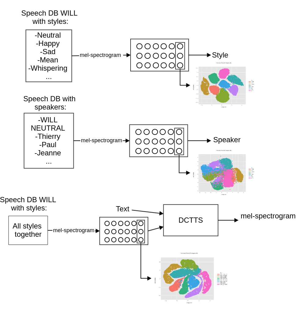
Figure 1: Illustration of data flow for the three embeddings computations systems. From top to bottom: Style classification system, speaker classification system and VAE-TTS.

3.1 Style Classification System

The classification system is a LSTM based DNN trained to predict the style category from audio features. The DNN consists of three LSTM layers (512/128/64 cells in each layer) and a fully connected 8-dim embedding layer. The input is 80-bin mel-spectrogram of utterances.

The generated embeddings capture discriminative information specific to the class it belongs to, in our case, the classes refer to the 8 styles of Will voice.

Similar to [18], training utterances are firstly segmented into fixed length chunks without silence and the embedding from the last frame is taken as the style embedding of the considered chunk.

In experiments, we tried different length chunks and found out that 800 ms gave the best classification performance. In the evaluation stage, we feed the whole utterance to the DNN to get the corresponding style embedding. Different from the speaker verification model in [19], our style classifier uses style labels directly to compute loss without calculating the cosine similarity matrix. As our interest is to investigate latent embeddings that help to design an expressive speech synthesis system, the top priority is to having embeddings that contain useful emotional or style information.

We obtained an accuracy of 94.38% on style classification in our evaluation stage on the 800 unseen utterances (100 utterance per style).

3.2 Speaker Classification System

As in Section 3.1, the speaker classification system is also a LSTM based DNN, but with four stacking LSTM with 512/512/512/64 cells in each layer, the 8-dim embedding layer is unchanged.

In this case, the system is trained to predict the speaker identity from audio features. The speaker classifier is trained with 276 speakers’ voices including the neutral subset of Will voice, the other styles of Will are not used during training.

The 276 speakers are composed of speakers of varying ages (from child to the elder), female/male, and varying personalities. Most speakers speak in a neutral way, but some of them speak in a quite unique manner. Moreover, the 276 speakers cover 35 languages, with half of them speaking English with various accents, like American English, UK English, Austrian English, etc. The second most speaking language is French. We would expect the embeddings generated from such a speaker classifier to reflect information not only about language, age, or gender , but also on prosody. As for the speaker classification system, utterances are firstly segmented into 800 ms chunks without silences in the training stage, and the entire utterance is fed to the classifier to get its embedding vector from the last non-silent frame. To train the classifier, we used as the training set 300 utterances per speaker and 100 utterances per speaker as the test set. Eventually we obtained 91.19% classification accuracy on the unseen test utterances.

3.3 VAE-TTS System

The TTS system is a deep learning algorithm trained to predict a spectrogram from the associated text input.

The TTS system used in this work is DCTTS [20]. DCTTS models a sequence-to-sequence task with a encoder-decoder structure coupled with an Attention Mechanism like Tacotron [21]. Contrary to Tacotron, the modules of the architecture do not contain any recurrent unit. It is only based on convolutional modules. This particularity makes it easier to train. In  [20], they compared an open source implementation of Tacotron  to DCTTS and report higher Mean Opinion Score (MOS).

In this work, we use the Tensorflow implementation available online .

There are two modules trained separately: Text2Mel and SSRN (for Spectrogram Super-resolution Network). Text2Mel does the mapping between character embeddings and the output of Mel Filter Banks (MFBs) applied on the audio signal, that is, a mel-spectrogram. Then the second module SSRN does the mapping between the mel-spectrogram and full resolution spectrogram. Finally, Griffin-Lim [22] is used as a vocoder.

Text2Mel module models the sequence-to-sequence task. It is composed of a Text Encoder, an Audio Encoder, an Attention Mechanism, and an Audio Decoder.

In this paper we built a extension of DCTTS similar to the extension of Tacotron described in [16].

We encode the mel-spectrogram into a vector and concatenate this vector to each character of the transcript embedding and train the system for TTS. We chose a size of 8 to be relatively small compared to mel-spectrogram size (80 bins). The goal is to have a bottleneck sufficiently narrow to avoid the network to learn to copy the input at output.

The embeddings are therefore trained to represent the remaining variance in audio that does not depend on text. There is no need for labels. This enables the use of audiobooks not annotated in ”style” or ”emotion” for training expressive speech synthesis systems.

4 Audio Analysis and Interpretation of Latent Spaces

Latent spaces computed in Section 3 should be useful to control a speech synthesis system. The goal is thus to have a latent space that has interpretable relationships with audio features that we could use to control in speech generation.

To that end, in Section 4.1 we evaluated the suitability of three embeddings for style classification. A good embedding must perform well in the classification task. Then we looked into the latent spaces in a closer detail.

This is investigated in Section 4.2 through an analysis of correlations between audio features and a linear approximation of these using embeddings.

In Section 4.3, we present a technique of 2D visualization of these relationships.

4.1 Style Classification score

Obviously, embeddings computed from the style classification system were trained to have a high classification score. Here we investigate the suitability of the two other embedding types for a style classification task. We measure their classification capacity in terms of mutual information, as shown in Table 2.It measures the dependency between each of the 8 embedding dimensions and style categories. Mutual information was computed with scikit-learn library [23].

Table 2: Mutual information (in bit) between embedding dimensions and style

	VAE-TTS	Style	Speaker
0	0.44	1.55	0.41
1	0.81	1.36	0.33
2	1.08	1.49	0.50
3	0.71	1.41	0.39
4	0.97	1.47	0.33
5	0.79	1.80	0.42
6	0.97	1.74	0.25
7	1.06	1.86	0.33

4.2 Relationship between the Embedding Spaces and Audio Features

In this analysis, we study the relationship between the embedding spaces and the eGeMAPS feature set [24]. This feature set was designed based on their potential to represent affective physiological changes in speech.

This analysis allows to investigate what features describe best the remaining variability in the data.

The procedure is the following:

• We approximate a linear function (i.e. hyperplane) between each latent space and the audio feature space with ordinary least squares linear regression.

• We compute the linear function approximations of audio features based on latent embeddings

• The goal is then to evaluate how the approximations correlate with ground truth values.

• To that aim, we compute the Absolute Pearson Correlation Coefficient (APCC) between predictions and ground truth

In other words, we compute the APCC between each audio feature and the best possible hyperplane, in terms of least squares, of each latent space.

To summarize these results, we present in Table 3 only features that have an $APCC>0.5$ in every latent space.

Table 3: APCC values between the best possible hyper-plan of each latent space and audio features of the eGeMAPS feature set

APCC	VAE-TTS	Style	Speaker
F0 mean	0.76	0.82	0.63
F0 percentile20.0	0.75	0.81	0.62
F0 percentile50.0	0.79	0.86	0.67
F0 percentile80.0	0.69	0.73	0.52
mfcc2 mean	0.73	0.77	0.65
mfcc4 mean	0.73	0.77	0.61
F1 freq mean	0.61	0.71	0.52
F2 freq mean	0.58	0.68	0.52
F3 freq mean	0.64	0.71	0.57
Alpha Ratio V mean	0.60	0.65	0.55
Hammarberg Index V mean	0.58	0.63	0.52
Slope V 0-500 mean	0.89	0.91	0.72
mfcc2 V mean	0.78	0.82	0.68
mfcc4 V mean	0.77	0.80	0.63

The feature set is based on Low-level descriptors (F0, formants, mfcc, etc.) to which are applied statistics for the utterance (mean, normalized standard deviation, percentiles). All functionals are applied to voiced regions only (non-zero F0). For MFCCs, there is also a version applied to all regions (voiced and unvoiced).

These features are defined in [24] as follows:

• F0: logarithmic F0 on a semitone frequency scale, starting at 27.5 Hz (semitone 0)

• F1-3: Formants 1 to 3 centre frequencies

• Alpha Ratio: ratio of the summed energy from 50-1000 Hz and 1-5 kHz

• Hammarberg Index: ratio of the strongest energy peak in the 0-2 kHz region to the strongest peak in the 2-5 kHz region.

• Spectral Slope 0-500 Hz and 500-1500 Hz: linear regression slope of the logarithmic power spectrum within the two given bands.

• mfcc1-4: Mel-Frequency Cepstral Coefficients 1 to 4

4.3 Dimensionality reduction of latent spaces

In this Section, we investigate the use of dimensionality reduction of latent spaces previously computed. Reducing the latent spaces to two dimensions will enable the possibility to design an interface that allows its visualization and its relationship with audio features.

To that aim, we use three different algorithms of dimensionality reduction: PCA, t-SNE and UMAP. We then perform the same procedure of regression as in Section 4.2 to obtain APCCs between each audio feature of Table 3 and the best possible hyper-plan, in terms of least squares, of each dimensionally reduced latent space.

Table 4 shows the average of APCCs for each pair (task, dimension reduction algorithm). For this pair, the gradients of hyper-plans approximating audio features were computed. The direction of these gradients correspond to the direction of the highest variation of a feature in the space. Figure 2 shows the reduced embeddings of all utterances of the dataset and the directions of the gradients.

This representation is useful for a perspective of interface for controllable speech synthesis system on which are represented the trends of audio features in the space.

Table 4: APCC average for each pair (task, dimensionality reduction algorithm)

APCC	PCA	t-SNE	UMAP
VAE-TTS	0.564	0.422	0.614
Style	0.480	0.366	0.607
Speaker	0.512	0.480	0.549

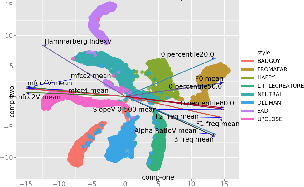
Figure 2: Latent space with directions of gradients of features listed in

5 Conclusions

This paper presents a methodology to build latent spaces related to style/emotion in speech and visualize it along with its relationships with important audio feature for a purpose of controllable speech synthesis.

To that aim, we compare three latent spaces computed by training deep learning-based systems on three different tasks. We then examined the potential of these latent spaces for style classification to confirm that they contain useful information for representing style.

We then studied the relationships between each latent space and audio features to obtain a sense of the impact of audio features on the expressed styles. This analysis consisted in an approximation of audio features from embeddings by linear regression. The accuracy of approximations was then evaluated in terms of correlations with ground truth.

The gradient of these linear approximations were computed to extract the information of variations of audio features in speech. By visualizing these gradients along with the embeddings, we observe the trends of audio features in the latent space.

In the future, this representation will be used to control an expressive speech synthesis system.

6 Acknowledgments

Noé Tits is funded through a PhD grant from the Fonds pour la Formation à la Recherche dans l’Industrie et l’Agriculture (FRIA), Belgium.

Thanks to Acapela Group for providing the dataset, for the interesting insights and collaboration on embeddings computation.

References

- [1] W.-N. Hsu, Y. Zhang, R. J. Weiss, H. Zen, Y. Wu, Y. Wang, Y. Cao, Y. Jia, Z. Chen, J. Shen et al., “Hierarchical generative modeling for controllable speech synthesis,” arXiv preprint arXiv:1810.07217, 2018.
- [2] G. E. Henter, X. Wang, and J. Yamagishi, “Deep encoder-decoder models for unsupervised learning of controllable speech synthesis,” arXiv preprint arXiv:1807.11470, 2018.
- [3] Y. Wang, D. Stanton, Y. Zhang, R. Skerry-Ryan, E. Battenberg, J. Shor, Y. Xiao, F. Ren, Y. Jia, and R. A. Saurous, “Style tokens: Unsupervised style modeling, control and transfer in end-to-end speech synthesis,” arXiv preprint arXiv:1803.09017, 2018.
- [4] P. Ekman, “An argument for basic emotions,” Cognition & emotion, vol. 6, no. 3-4, pp. 169–200, 1992.
- [5] S. R. Livingstone and F. A. Russo, “The ryerson audio-visual database of emotional speech and song (ravdess): A dynamic, multimodal set of facial and vocal expressions in north american english,” PLOS ONE, vol. 13, no. 5, pp. 1–35, 05 2018.
- [6] H. Cao, D. G. Cooper, M. K. Keutmann, R. C. Gur, A. Nenkova, and R. Verma, “Crema-d: Crowd-sourced emotional multimodal actors dataset,” IEEE transactions on affective computing, vol. 5, no. 4, pp. 377–390, 2014.
- [7] A. Adigwe, N. Tits, K. E. Haddad, S. Ostadabbas, and T. Dutoit, “The emotional voices database: Towards controlling the emotion dimension in voice generation systems,” arXiv preprint arXiv:1806.09514, 2018.
- [8] F. Burkhardt, A. Paeschke, M. Rolfes, W. F. Sendlmeier, and B. Weiss, “A database of german emotional speech,” in Ninth European Conference on Speech Communication and Technology, 2005.
- [9] N. Tits, K. E. Haddad, and T. Dutoit, “Exploring transfer learning for low resource emotional tts,” arXiv preprint arXiv:1901.04276, 2019.
- [10] Y. Lee, A. Rabiee, and S.-Y. Lee, “Emotional end-to-end neural speech synthesizer,” arXiv preprint arXiv:1711.05447, 2017.
- [11] J. A. Russell, “A circumplex model of affect.” Journal of personality and social psychology, vol. 39, no. 6, p. 1161, 1980.
- [12] C. Busso, S. Parthasarathy, A. Burmania, M. AbdelWahab, N. Sadoughi, and E. M. Provost, “Msp-improv: An acted corpus of dyadic interactions to study emotion perception,” IEEE Transactions on Affective Computing, vol. 8, no. 1, pp. 67–80, 2017.
- [13] C. Busso, M. Bulut, C.-C. Lee, A. Kazemzadeh, E. Mower, S. Kim, J. N. Chang, S. Lee, and S. S. Narayanan, “Iemocap: Interactive emotional dyadic motion capture database,” Language resources and evaluation, vol. 42, no. 4, p. 335, 2008.
- [14] G. A. Miller, “The magical number seven, plus or minus two: Some limits on our capacity for processing information.” Psychological review, vol. 63, no. 2, p. 81, 1956.
- [15] N. Tits, K. El Haddad, and T. Dutoit, “Asr-based features for emotion recognition: A transfer learning approach,” in Proceedings of Grand Challenge and Workshop on Human Multimodal Language (Challenge-HML). Association for Computational Linguistics, 2018, pp. 48–52. [Online]. Available: http://aclweb.org/anthology/W18-3307
- [16] R. Skerry-Ryan, E. Battenberg, Y. Xiao, Y. Wang, D. Stanton, J. Shor, R. J. Weiss, R. Clark, and R. A. Saurous, “Towards end-to-end prosody transfer for expressive speech synthesis with tacotron,” arXiv preprint arXiv:1803.09047, 2018.
- [17] K. Akuzawa, Y. Iwasawa, and Y. Matsuo, “Expressive speech synthesis via modeling expressions with variational autoencoder,” arXiv preprint arXiv:1804.02135, 2018.
- [18] Y. Jia, Y. Zhang, R. J. Weiss, Q. Wang, J. Shen, F. Ren, Z. Chen, P. Nguyen, R. Pang, I. L. Moreno et al., “Transfer learning from speaker verification to multispeaker text-to-speech synthesis,” arXiv preprint arXiv:1806.04558, 2018.
- [19] L. Wan, Q. Wang, A. Papir, and I. L. Moreno, “Generalized end-to-end loss for speaker verification,” in 2018 IEEE International Conference on Acoustics, Speech and Signal Processing (ICASSP). IEEE, 2018, pp. 4879–4883.
- [20] H. Tachibana, K. Uenoyama, and S. Aihara, “Efficiently trainable text-to-speech system based on deep convolutional networks with guided attention,” arXiv preprint arXiv:1710.08969, 2017.
- [21] Y. Wang, R. J. Skerry-Ryan, D. Stanton, Y. Wu, R. J. Weiss, N. Jaitly, Z. Yang, Y. Xiao, Z. Chen, S. Bengio, Q. V. Le, Y. Agiomyrgiannakis, R. Clark, and R. A. Saurous, “Tacotron: Towards end-to-end speech synthesis,” in INTERSPEECH, 2017.
- [22] D. Griffin and J. Lim, “Signal estimation from modified short-time fourier transform,” IEEE Transactions on Acoustics, Speech, and Signal Processing, vol. 32, no. 2, pp. 236–243, 1984.
- [23] F. Pedregosa, G. Varoquaux, A. Gramfort, V. Michel, B. Thirion, O. Grisel, M. Blondel, P. Prettenhofer, R. Weiss, V. Dubourg, J. Vanderplas, A. Passos, D. Cournapeau, M. Brucher, M. Perrot, and E. Duchesnay, “Scikit-learn: Machine learning in Python,” Journal of Machine Learning Research, vol. 12, pp. 2825–2830, 2011.
- [24] F. Eyben, K. R. Scherer, B. W. Schuller, J. Sundberg, E. André, C. Busso, L. Y. Devillers, J. Epps, P. Laukka, S. S. Narayanan et al., “The geneva minimalistic acoustic parameter set (gemaps) for voice research and affective computing,” IEEE Transactions on Affective Computing, vol. 7, no. 2, pp. 190–202, 2016.