A Control-Theoretic Approach to Analysis and Parameter Selection of Douglas-Rachford Splitting

Abstract

Douglas-Rachford splitting and its equivalent dual formulation ADMM are widely used iterative methods in composite optimization problems arising in control and machine learning applications. The performance of these algorithms depends on the choice of step size parameters, for which the optimal values are known in some specific cases, and otherwise are set heuristically. We provide a new unified method of convergence analysis and parameter selection by interpreting the algorithm as a linear dynamical system with nonlinear feedback. This approach allows us to derive a dimensionally independent matrix inequality whose feasibility is sufficient for the algorithm to converge at a specified rate. By analyzing this inequality, we are able to give performance guarantees and parameter settings of the algorithm under a variety of assumptions regarding the convexity and smoothness of the objective function. In particular, our framework enables us to obtain a new and simple proof of the $O(1/k)$ convergence rate of the algorithm when the objective function is not strongly convex.

I Introduction

In this paper, we consider problems of the form

$$\mathrm{minimize}_{x\in\mathbb{R}^{d}}\ \{F(x)=f(x)+g(x)\},$$ (1)

where $f,g:\mathbb{R}^{d}\to\mathbb{R}\cup\{+\infty\}$ are convex, closed, and proper (c.c.p.). Douglas-Rachford splitting (DRS) solves problem (1) with the following iterations:

$$y_{k} =\mathrm{prox}_{\alpha f}(x_{k}),$$ (2a)

$$z_{k} =\mathrm{prox}_{\alpha g}(2y_{k}-x_{k}),$$ (2b)

$$x_{k+1} =x_{k}+\lambda_{k}(z_{k}-y_{k}),$$ (2c)

where $\mathrm{prox}$ is the proximal operator (see Definition 1) and $\alpha$ and $\lambda_{k}$ are known as the proximal step size and relaxation parameter, respectively. For a proper selection of these parameters, the limiting values of both $y_{k}$ and $z_{k}$ will be a solution to (1). The goal of this work is to provide convergence rates for DRS over various assumptions on $f$ and $g$, and optimize these rates with respect to the algorithm parameters $\alpha$ and $\lambda_{k}$ using semidefinite programs (SDPs).

The algorithm was first proposed in [1], and has since found application in general separable optimization problems [2]. Its dual formulation, ADMM, has been particularly useful in distributed optimization problems [3]. Since the iterates of ADMM can be written as applying DRS to the dual problem [4, 5], convergence results for one algorithm are valid for the other as well when strong duality holds.

The convergence of DRS has previously been analyzed using monotone operator theory and variational inequalities, see [6], [7]. These techniques have led to proofs of a $O(1/k)$ convergence rate for the non-strongly convex case [8], and linear convergence when $f$ is smooth and strongly convex [9], [10]. In the most general case, a condition for convergence is that $\lambda_{k}\in(0,2)$ with $\sum_{k=0}^{\infty}\lambda_{k}(2-\lambda_{k})=\infty$ [11], though there exist cases where the algorithm converges with $\lambda_{k}>2$ [12].

Recently, there has been interest in automating the analysis and design of optimization algorithms via SDPs, [13, 14, 15, 16, 17, 18, 19]. In particular, through the method of integral quadratic constraints proposed in [14], the authors of [12] derive an SDP for choosing the parameters of ADMM in the case of smooth and strongly convex $f$. Using a similar framework, the authors of [20] provide evidence that as the relaxation parameter approaches $2$ from below, the linear convergence rate is close to being optimal and in [21] are able to analytically solve the SDP to give a convergence rate. The work in [22] gives an optimal choice for the relaxation parameter when $f$ is quadratic. Furthermore, [23] gives a set of assumptions in which a bound on the linear convergence rate is minimized by setting $\lambda_{k}=2$.

Our Contribution: By viewing DRS as a linear system with non-linear feedback, we derive a dimensionally independent matrix inequality which gives convergence guarantees via Lyapunov functions. Whereas such an approach was previously applied in [12] to the case of smooth and strongly convex $f$, our framework is novel in that it encompasses varying assumptions on the smoothness and convexity of $f$. By changing a single term in the Lyapunov function for each scenario, we are able to relate the satisfaction of a matrix inequality to the convergence of the algorithm. In particular, we give a new and simple proof of $O(1/k)$ convergence in the non-strongly convex case. These symbolic results can then be used to select step sizes that optimize the derived rates.

In the strongly convex case, the corresponding matrix inequality is sufficient to guarantee a linear convergence rate. We are able to modify the matrix inequality to linearize the dependence on $\lambda_{k}$, allowing us to numerically optimize its value for the convergence rate directly. While previous work derived SDP’s which can verify the performance of the algorithm for a given parameter setting, to the best of our knowledge this is the first time such a method immediately gives an optimal relaxation parameter when solved numerically, as opposed to having to search over a range of values for $\lambda_{k}$.

II Preliminaries

We denote the set of real numbers by $\mathbb{R}$, the set of real $n$-dimensional vectors by $\mathbb{R}^{n}$, the set of real $m\times n$-dimensional matrices by $\mathbb{R}^{m\times n}$, and the $n$-dimensional identity matrix and zero matrix by $I_{n}$ and $0_{n}$, respectively. For a function $f\colon\mathbb{R}^{d}\to\mathbb{R}\cup\{+\infty\}$, we denote by $\mathrm{dom}\,f=\{x\in\mathbb{R}^{d}\colon f(x)<\infty\}$ the effective domain of $f$. The subdifferential of a function $f$ at a point $x$ is $\partial f(x):=\{g\;|\;f(y)-f(x)\geq g^{\top}(y-x),\forall y\in\mathrm{dom}(f)\}$. By abuse of notation we will also refer to a subgradient, that is an element of the subdifferential by $\partial f(x)$ as well. The indicator function of a set $C$ is given by $\mathrm{1}_{C}(x)=0$ if $x\in C$ and $\mathrm{1}_{C}(x)=\infty$ if $x\notin C$. For two matrices $A\in\mathbb{R}^{m\times n}$ and $B\in\mathbb{R}^{p\times q}$ their Kronecker product is $A\otimes B$.

We say a differentiable function $f\colon\mathbb{R}^{d}\to\mathbb{R}$ is $L_{f}$-smooth on $\mathcal{S}\subseteq\mathrm{dom}\,f$ if $\|\nabla f(x)-\nabla f(y)\|_{2}\leq L_{f}\|x-y\|_{2}$ for some $L_{f}>0$ and all $x,y\in\mathcal{S}$. This also implies for all $x,y\in\mathcal{S}$, $f(y)\leq f(x)+\nabla f(x)^{\top}(y-x)+(L_{f}/2)\|y-x\|_{2}^{2}$. A differentiable function $f\colon\mathbb{R}^{d}\to\mathbb{R}$ is $m_{f}$-strongly convex on $\mathcal{S}\subseteq\mathrm{dom}\,f$ if $m_{f}\|x-y\|_{2}^{2}\leq(x-y)^{\top}(\nabla f(x)-\nabla f(y))$ for some $m_{f}>0$ and all $x,y\in\mathcal{S}$. The class of functions which are $L_{f}$-smooth and $m_{f}$-strongly convex is denoted by $\mathcal{F}(m_{f},L_{f})$.

Definition 1 (Proximal Operator)

Given a c.c.p. function $f:\mathbb{R}^{d}\to\mathbb{R}\cup\{+\infty\}$ and $\alpha>0$, the proximal operator $\mathrm{prox}_{\alpha f}:\mathbb{R}^{d}\to\mathbb{R}^{d}$ is defined as

$$\mathrm{prox}_{\alpha f}(x)=\text{argmin}_{y}\left\{f(y)+\frac{1}{2\alpha}\|x-y\|_{2}^{2}\right\}.$$ (3)

The point $y=\mathrm{prox}_{\alpha f}(x)$ also is given by the implicit solution to the subgradient equation

$$y=x-\alpha\partial f(y).$$ (4)

We say that a nonlinear function $\phi:\mathbb{R}^{d}\to\mathbb{R}^{d}$ satisfies the incremental quadratic constraint [24] (or point-wise integral quadratic constraint [14]) defined by $Q\in\mathbb{R}^{2d\times 2d}$ if for all $x,y$,

$$\begin{bmatrix}x\!-\!y\\ \phi(x)\!-\!\phi(y)\end{bmatrix}^{\top}\!Q\!\begin{bmatrix}x\!-\!y\\ \phi(x)\!-\!\phi(y)\end{bmatrix}\geq 0.$$ (5)

For $0\leq m,L<\infty$ define

$$Q(m,L)=\begin{bmatrix}-\frac{mL}{m+L}&1/2\\ 1/2&-\frac{1}{m+L}\end{bmatrix}\otimes I_{d},$$ (6)

and define $Q(m,\infty)$ as $\lim_{L\to\infty}Q(m,L)$. It was noted in [25, 14] that a differentiable function $f$ belongs to the class $\mathcal{F}(m_{f},L_{f})$ on $\mathcal{S}$ if and only if the gradient $\nabla f$ satisfies the incremental QC defined by $Q(m_{f},L_{f})$. When $L_{f}=\infty$, the subgradient $\partial f$ satisfies the QC defined by $Q(m_{f},\infty)$. If we define

$$Q_{p}(m,L,\alpha)=\begin{bmatrix}0&I_{d}\\ \alpha I_{d}&-I_{d}\end{bmatrix}Q(m,L)\begin{bmatrix}0&\alpha I_{d}\\ I_{d}&-I_{d}\end{bmatrix},$$ (7)

then the proximal operator of a function $f\in\mathcal{F}(m,L)$, $\mathrm{prox}_{\alpha f}$, satisfies the incremental QC defined by $Q_{p}(m,L,\alpha)$ [15].

III Analysis of Douglas-Rachford Splitting via Matrix Inequalities

III-A Douglas-Rachford Splitting as a Dynamical System

We can write the updates in (2) as a linear system with state $x_{k}$ and feedback nonlinearity $\phi(x_{k})$,

$$x_{k+1}=x_{k}+\lambda_{k}\phi(x_{k}),$$ (8)

where

$$\phi(x_{k}):=\mathrm{prox}_{\alpha g}(2\mathrm{prox}_{\alpha f}(x_{k})-x_{k})-\mathrm{prox}_{\alpha g}(x_{k}).$$ (9)

Our main technique is to describe the nonlinearity $\phi$ with incremental QCs representing the $\mathrm{prox}$ operator. This allows us to derive a matrix inequality as a sufficient condition for closed-loop stability of the system via a Lyapunov function argument. We perform this derivation in the following three cases:

• Case 1: $f\in\mathcal{F}(0,\infty)$ and $g\in\mathcal{F}(0,\infty)$,

• Case 2: $f\in\mathcal{F}(0,L_{f})$ and $g\in\mathcal{F}(0,\infty)$, with $0<L_{f}<\infty$,

• Case 3: $f\in\mathcal{F}(m_{f},L_{f})$ and $g\in\mathcal{F}(0,\infty)$, with $0<m_{f}\leq L_{f}<\infty$.

We will see that for each case only one term in the Lyapunov function needs to be modified to obtain the convergence result. We then use the matrix inequality condition for each case to obtain information about optimal choices of the algorithm parameters both symbolically and numerically.

III-B Characterization of Fixed Points

From relation (4), the iterates (2) can be rewritten as

$$y_{k} =x_{k}-\alpha\partial f(y_{k}),$$ (10a)

$$z_{k} =2y_{k}-x_{k}-\alpha\partial g(z_{k}),$$ (10b)

$$x_{k+1} =x_{k}+\lambda_{k}(z_{k}-y_{k}).$$ (10c)

The fixed points of (10) satisfy

$$x_{\star}=y_{\star}\!+\!\alpha\partial f(y_{\star}),\ y_{\star}=z_{\star},\ \partial f(y_{\star})\!+\!\partial g(z_{\star})=0.$$ (11)

Since $y_{\star}=z_{\star}$, the rightmost equality is exactly the optimality condition for (1).

We will also make use of the following relation, obtained from adding the equations in (10) and the definition of $\phi$,

$$\phi(x_{k})=z_{k}-y_{k}=-\alpha(\partial f(y_{k})+\partial g(z_{k})).$$ (12)

From this, we can interpret the feedback nonlinearity $\phi$ as the optimality residual of problem (1), which is driven to zero by the linear system in the feedback interconnection.

III-C Convergence Certificates via Matrix Inequalities

III-C1 Case 1: Non-strongly convex and non-smooth case

We first assume that $f,g\in\mathcal{F}(0,\infty)$. We propose the following family of Lyapunov functions parameterized by a sequence $\{\theta_{i}\}_{i=0}^{\infty}$ with $\theta_{i}>0$,

$$V_{k}\!=\!\|x_{k}-x_{\star}\|_{2}^{2}+\sum_{i=0}^{k-1}\theta_{i}\|\partial f(y_{i})+\partial g(z_{i})\|_{2}^{2},$$ (13)

for all $k>0$ and $V_{0}=\|x_{0}-x_{\star}\|^{2}$. For notational convenience define the partial sums $\Theta_{k}=\sum_{i=0}^{k-1}\theta_{i}$. The presence of the running sum of subgradients is reminiscent of the Popov criterion [26]. It can also be interpreted as the running weighted sum of fixed point residuals (see (11)). The next lemma shows how this Lyapunov function can ensure a convergence rate in terms of the growth of $\Theta_{k}$.

Lemma 1

Consider the algorithm in (2). Suppose there exists a sequence $\{\theta_{i}\}_{i=0}^{\infty}$ with $\theta_{i}>0$ such that $V_{k+1}\leq V_{k}$ for all $k\geq 0$. Then

$$\min_{i=0,\ldots,k-1}\|\partial f(y_{i})+\partial g(z_{i})\|_{2}^{2}\leq\frac{1}{\Theta_{k}}\|x_{0}-x_{\star}\|_{2}^{2}.$$ (14)

Proof:

Since $V_{k+1}\leq V_{k}$ for all $k$, in particular we have that $V_{k}\leq V_{0}$, or

$$\|x_{k}\!-\!x_{\star}\|_{2}^{2}\!+\!\!\sum_{i=0}^{k-1}\theta_{i}\|\partial f(y_{i})\!+\!\partial g(z_{i})\|_{2}^{2}\leq\|x_{0}-x_{\star}\|_{2}^{2}.$$ (15)

Removing the first term on the left, and dividing through by $\Theta_{k}$ gives

$$\sum_{i=0}^{k-1}\frac{\theta_{i}}{\Theta_{k}}\|\partial f(y_{i})+\partial g(z_{i})\|_{2}^{2}\leq\dfrac{\|x_{0}-x_{\star}\|_{2}^{2}}{\Theta_{k}}.$$ (16)

The result follows from the fact that the left side is a weighted average, as $\theta_{i}>0$ and $\sum_{i=0}^{k-1}\theta_{i}/\Theta_{k}=1$. ∎

In the following theorem, we derive a matrix inequality in terms of $\alpha,\lambda$, and $\{\theta_{i}\}_{i=0}^{\infty}$ as a sufficient condition to guarantee $V_{k+1}\leq V_{k}$, which in turn implies (14).

Theorem 1

Let $m_{f}=0$, $L_{f}=\infty$, and consider the following matrix inequality

$$W_{k}^{(0)}+\sigma_{k}^{(1)}Q^{(1)}+\sigma_{k}^{(2)}Q^{(2)}\preceq 0,$$ (17)

where

$$W_{k}^{(0)} =\begin{bmatrix}0&-\lambda_{k}&\lambda_{k}\\ -\lambda_{k}&\lambda_{k}^{2}+\frac{\theta_{k}}{\alpha^{2}}&-\left(\lambda_{k}^{2}+\frac{\theta_{k}}{\alpha^{2}}\right)\\ \lambda_{k}&-\left(\lambda_{k}^{2}+\frac{\theta_{k}}{\alpha^{2}}\right)&\lambda_{k}^{2}+\frac{\theta_{k}}{\alpha^{2}}\end{bmatrix}\!\otimes\!I_{d},$$ (18a)

$$Q^{(1)} =\begin{bmatrix}0&I_{d}\\ \alpha I_{d}&-I_{d}\\ 0&0\end{bmatrix}Q(m_{f},L_{f})\begin{bmatrix}0&\alpha I_{d}&0\\ I_{d}&-I_{d}&0\end{bmatrix},$$ (18b)

$$Q^{(2)} =\begin{bmatrix}0&-I_{d}\\ 0&2I_{d}\\ \alpha I_{d}&-I_{d}\end{bmatrix}\!Q(0,\infty)\!\begin{bmatrix}0\!&0\!&\alpha I_{d}\!\\ -I_{d}\!&2I_{d}\!&-I_{d}\!\end{bmatrix}.$$ (18c)

If $\alpha,\lambda_{k},\theta_{k}>0$ and $\sigma_{k}^{(1)},\sigma_{k}^{(2)}\geq 0$ are chosen so that (17) is satisfied for all $k\geq 0$, then for all $f\in\mathcal{F}(0,\infty)$ and $g\in\mathcal{F}(0,\infty)$ the iterates in (2) satisfy

$$\min_{i=0,\ldots,k-1}\|\partial f(y_{i})+\partial g(z_{i})\|_{2}^{2}\leq\frac{1}{\Theta_{k}}\|x_{0}-x_{\star}\|_{2}^{2}.$$ (19)

Proof:

We first see that $V_{k+1}-V_{k}$ can be written as a quadratic form. Define the error signal

$$e_{k}:=\begin{bmatrix}(x_{k}-x_{\star})^{\top}&(y_{k}-y_{\star})^{\top}&(z_{k}-z_{\star})^{\top}\end{bmatrix}^{\top}.$$ (20)

Using the updates in (10), the fact that $z_{\star}=y_{\star}$ (see (11)), and the relation (12), it can be verified that

$$V_{k+1}-V_{k}=e_{k}^{\top}W_{k}^{(0)}e_{k},$$ (21)

where $W_{k}^{(0)}$ is given by (18a). Next, note that

$$e_{k}^{\top}Q^{(1)}e_{k}=\begin{bmatrix}x_{k}-x_{\star}\\ y_{k}-y_{\star}\end{bmatrix}^{\top}Q_{p}(m_{f},L_{f},\alpha)\begin{bmatrix}x_{k}-x_{\star}\\ y_{k}-y_{\star}\end{bmatrix},$$ (22)

where $Q_{p}(m_{f},L_{f},\alpha)$ is defined in (7). Since $y_{k}=\mathrm{prox}_{\alpha f}(x_{k})$ and $y_{\star}=\mathrm{prox}_{\alpha f}(x_{\star})$, this is exactly the incremental QC that the $\mathrm{prox}_{\alpha f}$ operator satisfies. Thus, we have for all $k$, $e_{k}^{\top}Q^{(1)}e_{k}\geq 0$. We also note that

$$\begin{bmatrix}0\!&\!0&\!\alpha I_{d}\!\\ -I_{d}\!&2I_{d}\!&-I_{d}\!\end{bmatrix}e_{k}\!=\!\begin{bmatrix}0\!&\!\alpha\!I_{d}\!\\ I_{d}\!&-I_{d}\!\end{bmatrix}\!\begin{bmatrix}(2y_{k}\!-\!x_{k})\!-\!(2y_{\star}\!-\!x_{\star})\!\\ z_{k}-z_{\star}\end{bmatrix}.$$

As $z_{k}=\mathrm{prox}_{\alpha g}(2y_{k}-x_{k})$ and $z_{\star}=\mathrm{prox}_{\alpha g}(2y_{\star}-x_{\star})$, we similarly conclude that $e_{k}^{\top}Q^{(2)}e_{k}\geq 0$ is implied from the incremental QC that $\mathrm{prox}_{\alpha g}$ satisfies. Returning to (17), if we multiply from the left and right by $e_{k}^{\top}$ and $e_{k}$ respectively, we obtain

$$e_{k}^{\top}W_{k}^{(0)}e_{k}+\sigma_{k}^{(1)}e_{k}^{\top}Q^{(1)}e_{k}+\sigma_{k}^{(2)}e_{k}^{\top}Q^{(2)}e_{k}\leq 0.$$ (23)

Since $\sigma_{k}^{(1)},\sigma_{k}^{(2)}\geq 0$ and we have shown that $e_{k}^{\top}Q^{(1)}e_{k}\geq 0$ and $e_{k}^{\top}Q^{(2)}e_{k}\geq 0$, it must be that $e_{k}^{\top}W_{k}^{(0)}e_{k}\leq 0$. Hence, $V_{k+1}\!-\!V_{k}\leq 0$, and the result now follows from Lemma 1. ∎

III-C2 Case 2: Non-strongly convex and smooth $f$

If $f\in\mathcal{F}(0,L_{f})$ with $0<L_{f}<\infty$, we may leverage the smoothness of $f$ to refine the result of the previous section. In particular, we can use the inequality for $L_{f}$-smooth functions (see Preliminaries) to relate the behavior of the subgradients to the objective values, whereas in the previous section this inequality was not available. For $k>0$ let

$$V_{k}=\|x_{k}-x_{\star}\|_{2}^{2}+\sum_{i=0}^{k-1}\theta_{i}[F(z_{i})-F(z_{\star})],$$ (24)

with $V_{0}$ defined as in the previous case.

This Lyapunov function leads to the following Lemma, the proof of which is identical to that of Lemma 1.

Lemma 2

Consider the algorithm in (2). Suppose there exists a sequence $\{\theta_{i}\}_{i=0}^{\infty}$ with $\theta_{i}>0$ such that $V_{k+1}\leq V_{k}$ for all $k\geq 0$. Then

$$\min_{i=0,\ldots,k-1}[F(z_{i})-F(z_{\star})]\leq\dfrac{1}{\Theta_{k}}\|x_{0}-x_{\star}\|_{2}^{2}.$$

This allows us to prove the following theorem for when $f$ is non-strongly convex and smooth.

Theorem 2

Let $0=m_{f}<L_{f}<\infty$ and consider the following matrix inequality

$$W_{k}^{(1)}+\sigma_{k}^{(1)}Q^{(1)}+\sigma_{k}^{(2)}Q^{(2)}\preceq 0,$$ (25)

where

$$W_{k}^{(1)}\!\!=\!\!\begin{bmatrix}0\!\!&-\lambda_{k}&\lambda_{k}\\ -\lambda_{k}\!\!&\frac{\theta_{k}L_{f}}{2}+\lambda_{k}^{2}&\frac{\theta_{k}}{2}\left(\frac{1}{\alpha}-L_{f}\right)\!-\!\lambda_{k}^{2}\\ \lambda_{k}\!\!&\frac{\theta_{k}}{2}\!\left(\frac{1}{\alpha}\!-\!L_{f}\right)\!-\!\lambda_{k}^{2}&\theta_{k}\left(\frac{L_{f}}{2}-\frac{1}{\alpha}\right)\!+\!\lambda_{k}^{2}\end{bmatrix}\!\otimes\!I_{d},$$ (26)

and $Q^{(1)}$ and $Q^{(2)}$ are defined in (18). If $\alpha,\lambda_{k},\theta_{k}>0$ and $\sigma_{k}^{(1)},\sigma_{k}^{(2)}\geq 0$ are chosen so that (25) is satisfied for all $k\geq 0$, then for all $f\in\mathcal{F}(0,L_{f})$ with $0<L_{f}<\infty$ and $g\in\mathcal{F}(0,\infty)$ the iterates in (2) satisfy

$$\min_{i=0,\ldots,k-1}[F(z_{i})-F(z_{\star})]\leq\frac{1}{\Theta_{k}}\|x_{0}-x_{\star}\|_{2}^{2}.$$ (27)

Proof:

We begin by bounding the difference of the Lyapunov function defined in (24), $V_{k+1}-V_{k}$, by a quadratic form in the error signal $e_{k}$ (see (20)). From the convexity and smoothness of $f$, we can write

$$f(z_{k})\!-\!f(y_{k})\! \leq\nabla f(y_{k})^{\top}(z_{k}\!-\!y_{k})+\frac{L_{f}}{2}\|z_{k}-y_{k}\|_{2}^{2},$$ (28)

$$f(y_{k})\!-\!f(z_{\star})\! \leq\nabla f(y_{k})^{\top}(y_{k}\!-\!y_{\star}),$$ (29)

where we have used that $z_{\star}=y_{\star}$. From the convexity of $g$

$$g(z_{k})-g(z_{\star})\leq\partial g(z_{k})^{\top}(z_{k}-z_{\star}).$$ (30)

Adding these three inequalities together and using the relation (12) allows us to conclude

$$F(z_{k})-F(z_{\star}) \leq\frac{L_{f}}{2}\|y_{k}-y_{\star}\|_{2}^{2}+\left(\frac{L_{f}}{2}-\frac{1}{\alpha}\right)\|z_{k}-z_{\star}\|_{2}^{2}$$

$$\quad+\left(\frac{1}{\alpha}-L_{f}\right)(y_{k}-y_{\star})^{\top}(z_{k}-z_{\star}).$$ (31)

Using the recursion for $x_{k+1}$, we then find that

$$V_{k+1}-V_{k}\leq e_{k}^{\top}W_{k}^{(1)}e_{k}.$$ (32)

The proof now proceeds identically as in the proof of Theorem 1 up to the statement that (25) implies $e_{k}^{\top}W_{k}^{(1)}e_{k}\leq 0$. Then by (32), we have that $V_{k+1}-V_{k}\leq 0$, and the result follows from Lemma 2. ∎

III-C3 Case 3: Strongly convex and smooth $f$

We now assume that $f\in\mathcal{F}(m_{f},L_{f})$ and $g\in\mathcal{F}(0,\infty)$, with $0<m_{f}\leq L_{f}<\infty$. For this scenario let

$$V_{k}=\|x_{k}-x_{\ast}\|_{2}^{2}.$$ (33)

The following lemma characterizes when we can extract a linear convergence rate from this Lyapunov function.

Lemma 3

Consider the algorithm in (2). Suppose there exists $\rho\in(0,1)$ such the Lyapunov function $V_{k}$ defined by (33) satisfies $V_{k+1}\leq\rho^{2}V_{k}$ for all $k\geq 0$. Then

$$\|x_{k}-x_{\ast}\|_{2}^{2}\leq\rho^{2k}\|x_{0}-x_{\ast}\|_{2}^{2}.$$ (34)

Proof:

The proof follows immediately $V_{k+1}\leq\rho^{2}V_{k}$, the definition (33) of $V_{k}$, and induction. ∎

We again see that the difference $V_{k+1}-\rho^{2}V_{k}$ can be written as a quadratic form acting on the error signal $e_{k}$ as defined in (20). Using the definition for $x_{k+1}$ in terms of the previous iterates, we can write

$$V_{k+1}-\rho^{2}V_{k}=e_{k}^{\top}Q_{k}e_{k},$$ (35)

where $Q_{k}$ is given by

$$Q_{k}=\begin{bmatrix}1-\rho^{2}&-\lambda_{k}&\lambda_{k}\\ -\lambda_{k}&\lambda_{k}^{2}&-\lambda_{k}^{2}\\ \lambda_{k}&-\lambda_{k}^{2}&\lambda_{k}^{2}\end{bmatrix}\otimes I_{d}.$$ (36)

From (35), we can use the same reasoning developed in the non-strongly convex case to arrive at the following theorem.

Theorem 3

Let $0<m_{f}\leq L_{f}<\infty$ and consider the following matrix inequality

$$Q_{k}+\sigma_{k}^{(1)}Q^{(1)}+\sigma_{k}^{(2)}Q^{(2)}\preceq 0,$$ (37)

where $Q_{k}$ is given in (36) and $Q^{(1)}$ and $Q^{(2)}$ are given in (18). If $\alpha,\lambda_{k}>0$, $\sigma_{k}^{(1)},\sigma_{k}^{(2)}\geq 0$, and $\rho\in(0,1)$ are chosen so that (37) is satisfied for all $k\geq 0$, then for all $f\in\mathcal{F}(m_{f},L_{f})$ and $g\in\mathcal{F}(0,\infty)$ with $0<m_{f}\leq L_{f}<\infty$, the iterates in (2) satisfy the following linear convergence rate

$$\|x_{k}-x_{\ast}\|_{2}^{2}\leq\rho^{2k}\|x_{0}-x_{\ast}\|_{2}^{2}.$$ (38)

Proof:

We proceed identically as in the proof of Theorems 1 and 2. If (37) is satisfied, then $e_{k}^{\top}Q_{k}e_{k}\leq 0$ for all $k$. This is equivalent to $V_{k+1}-\rho^{2}V_{k}\leq 0$, by which (38) follows from Lemma 3. ∎

IV Optimizing the Bound and Relaxation Parameter

For each of the cases presented in the previous section we use the associated matrix inequality to optimize our bounds on the convergence rate. In the case of non-strongly convex $f$ we provide analytic convergence rates, while for strongly convex $f$ we optimize our bounds numerically.

IV-1 Case 1: Non-strongly convex and non-smooth case

We now select algorithm parameters that satisfy the matrix inequality in (17). In doing so, we arrive at a new and simple proof of the $O(1/k)$ convergence of DRS in the non-strongly convex and non-smooth case.

Theorem 4

If $f\in\mathcal{F}(0,\infty)$ and $g\in\mathcal{F}(0,\infty)$, then for any choice of $\lambda_{k}=\lambda\in(0,2)$ and $\alpha>0$, if we set $\sigma_{k}^{(1)}=\sigma_{k}^{(2)}=\sigma_{k}$, with

$$\sigma_{k}:=2\lambda_{k}/\alpha,\quad\theta_{k}:=\alpha^{2}\lambda_{k}(2-\lambda_{k}),$$ (39)

then $\sigma_{k}^{(1)},\sigma_{k}^{(2)},\alpha,\lambda_{k},$ and $\theta_{k}$ satisfy the matrix inequality (17).

Proof:

Making these substitutions gives $W_{k}^{(0)}+\sigma_{k}^{(1)}Q^{(1)}+\sigma_{k}^{(2)}Q^{(2)}=0_{n}\preceq 0.$ ∎

Remark 1

The convergence rate bound provided by the parameter choices in Theorem 4 guarantees convergence only if $\lim_{k\to\infty}\Theta_{k}=\infty$, which in this case means $\sum_{i=0}^{\infty}\lambda_{k}(2-\lambda_{k})=\infty$. This is consistent with the conditions on the relaxation parameter found in [11].

Remark 2

After setting $\theta_{k}$ as in (39), we can maximize $\Theta_{k}$ by setting $\lambda_{k}=1$ which results in $\Theta_{k}=\alpha^{2}k$ and the following result

$$\min_{i=0,\ldots,k-1}\|\partial f(y_{i})+\partial g(z_{i})\|_{2}^{2}\leq\frac{1}{\alpha^{2}k}\|x_{0}-x_{\star}\|_{2}^{2}.$$ (40)

Remark 3

Using the relation (12) we can rewrite (40) as

$$\min_{i=0,\ldots,k-1}\|z_{i}-y_{i}\|_{2}^{2}\leq\frac{1}{k}\|x_{0}-x_{\star}\|_{2}^{2}.$$ (41)

Thus we see that Theorem 4 also gives a $O(1/k)$ rate toward the iterates being a fixed point of the algorithm.

IV-2 Case 2: Non-strongly convex and smooth case

When $f\in\mathcal{F}(0,L_{f}),g\in\mathcal{F}(0,\infty)$ with $0<L_{f}<\infty$, we have the following result on feasibility of the matrix inequality (25).

Theorem 5

For any $\alpha>0$ and $\lambda_{k}=\lambda$ with $0<\lambda<2$, if we set $\sigma_{k}^{(1)}=\sigma_{k}^{(2)}=\sigma_{k}$,

$$\sigma_{k} :=\frac{2\lambda_{k}}{\alpha}\left(\sqrt{\left(\frac{2-\lambda_{k}}{\alpha L_{f}}\right)^{2}+1}-\left(\frac{2-\lambda_{k}}{\alpha L_{f}}\right)\right),$$ (42a)

$$\theta_{k} :=2\lambda_{k}\alpha\!\left(1\!+\!\left(\frac{2-\lambda_{k}}{\alpha L_{f}}\right)\!-\!\sqrt{\left(\frac{2-\lambda_{k}}{\alpha L_{f}}\right)^{2}\!+\!1}\right).$$ (42b)

Then $\sigma_{k}^{(1)},\sigma_{k}^{(2)},\alpha,\lambda_{k}$, and $\theta_{k}$ satisfy the matrix inequality (25).

Proof:

This can be verified by substituting the expressions for $\sigma_{k}^{(1)}$, $\sigma_{k}^{(2)}$, and $\theta_{k}$ into the minors of $W_{k}^{(1)}+\sigma_{k}^{(1)}Q^{(2)}+\sigma_{k}^{(2)}Q^{(2)}$ and seeing that Sylverster’s criterion is satisfied [27]. ∎

Remark 4

Note that for a constant selection of $\theta_{k}=\theta$, $\Theta_{k}=\theta k$. If (25) holds then

$$\min_{i=0,\ldots,k-1}[F(z_{i})-F(z_{\star})]\leq\dfrac{1}{\theta k}\|x_{0}-x_{\star}\|_{2}^{2}.$$ (43)

Remark 5

For moderate values of $\alpha L_{f}$, we can take a second order Taylor expansion of the rightmost term in (42b) and maximize the resulting expression with respect to $\lambda_{k}$. This suggests that we should set $\lambda_{k}$ to

$$\lambda_{k}=\frac{2}{3}\left(2-\alpha L_{f}+\sqrt{1-\alpha L_{f}+\alpha^{2}L_{f}^{2}}\right).$$ (44)

IV-3 Case 3: Strongly convex and smooth case

When $f\in\mathcal{F}(m_{f},L_{f})$, $g\in\mathcal{F}(0,\infty)$, with $0<m_{f}\leq L_{f}<\infty$, we can modify the matrix inequality (37) to get a linear dependence on the relaxation parameter. If we define $\Lambda_{k}:=\begin{bmatrix}0&-\lambda_{k}&\lambda_{k}\end{bmatrix}^{\top}\otimes I_{d}$ and

$$M_{k}:=(Q_{k}-\Lambda_{k}\Lambda_{k}^{\top})+\sigma_{k}^{(1)}Q^{(1)}+\sigma_{k}^{(2)}Q^{(2)},$$ (45)

then (37) is equivalent to

$$M_{k}-\Lambda_{k}[-1]\Lambda_{k}^{\top}\preceq 0.$$ (46)

As $\Lambda_{k}\Lambda_{k}^{\top}\succeq 0$, if (46) is satisfied then it must be the case that $M_{k}\preceq 0$. We now recognize that $M_{k}-\Lambda_{k}[-1]\Lambda_{k}^{\top}$ is the Schur Complement of the bottom right entry in the matrix

$$\Sigma_{k}:=\begin{bmatrix}M_{k}&\Lambda_{k}\\ \Lambda_{k}^{\top}&-1\end{bmatrix}.$$ (47)

By the properties of the Schur complement [28], we can conclude that (37) is satisfied if and only if $\Sigma_{k}\preceq 0$. The advantage of using $\Sigma_{k}\preceq 0$ instead of (37), is that now both the convergence rate $\rho^{2}$ and the relaxation parameter $\lambda_{k}$ appear linearly. If we set $\sigma_{k}^{(1)}=\sigma^{(1)}$, $\sigma_{k}^{(2)}=\sigma^{(2)}$, and $\lambda_{k}=\lambda$ for all $k$, the corresponding bound in (38) can be optimized by solving the following SDP, where $\lambda$ is now a decision variable,

$$\text{minimize}\quad\rho^{2},\quad\text{subject to}\quad\Sigma_{k}\preceq 0,$$ (48)

where the decision variables are $\rho^{2},\lambda>0$ and $\sigma^{(1)},\sigma^{(2)}\geq 0$. The optimal $\rho^{2}$ from solving this program over a range of step sizes $\alpha$ and condition numbers $\kappa_{f}=L_{f}/m_{f}$ is shown in Figure 1. We see that with increasing $\kappa_{f}$, the optimal choice of $\alpha$ decreases. Across the range of values of $\kappa_{f}$ and $\alpha$, the SDP (48) returns $\lambda=2$ as the optimal relaxation parameter.

Remark 6

We may repeat the same derivation for the inequalities (17) and (25) to linearize their dependence on $\lambda_{k}$ as well.

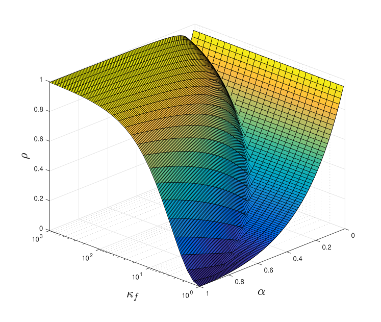
Figure 1: Optimal upper bound to linear convergence rate $\rho$ over $f\in\mathcal{F}(m_{f},L_{f})$, $g\in\mathcal{F}(0,\infty)$ as a function of step size $\alpha$ and condition number $\kappa_{f}=L_{f}/m_{f}$.

V Numerical Experiments

We investigate how our theoretical results compare with the experimental performance of DRS in the three scenarios described above. For the non-smooth and non-strongly convex case, we consider a basis pursuit problem (see [3]),

$$\underset{x,z\in\mathbb{R}^{n}}{\text{minimize}} \quad\mathrm{1}_{\{y\in\mathbb{R}^{n}|Ay=b\}}(x)+\|z\|_{1}$$

subject to $$\quad x-z=0,$$

with data $A\in\mathbb{R}^{300\times 10000}$ and $b\in\mathbb{R}^{300}$. We run DRS on the dual of this problem (ADMM) which is non-smooth and non-strongly convex. We test the convergence over a range of values of $\lambda_{k}=\lambda$, including $\lambda^{\star}=1$ (see Remark 2), and fixed $\alpha=1$.

For the smooth cases we consider a LASSO problem,

$$\mathrm{minimize}_{x}\quad\frac{1}{2}\|Ax-b\|_{2}^{2}+\gamma\|x\|_{1}.$$

with $A\in\mathbb{R}^{300\times 200}$, $b\in\mathbb{R}^{300}$ and $\gamma=0.1$. For the non-strongly convex case we set $A$ to be rank deficient and plot the convergence of DRS over a range of $\alpha$ with $\lambda_{k}=1$ fixed. The value $\alpha^{\star}$ is found by performing a grid search over possible values and choosing that which maximizes the rate given by Theorem 2. For the strongly convex case $A$ is set to be full rank and plot the convergence of DRS over a range of $\alpha$ with $\lambda_{k}=2$ fixed. Again, $\alpha^{\star}$ is the value of $\alpha$ which gives the best rate as provided by Theorem 3. The results are presented in Figure 2.

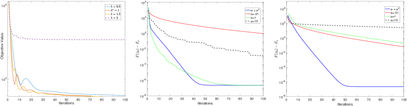
Figure 2: From left to right: convergence of DRS on basis pursuit problem with $\alpha=1$ and varying $\lambda$, convergence of DRS on LASSO problem with row-rank deficient $A$ with $\lambda=1$ and varying $\alpha$, convergence of DRS on LASSO problem with full row-rank $A$ with fixed $\lambda=2$ and varying $\alpha$.

VI Conclusion

We presented a unified framework for deriving convergence bounds for DRS and parameter settings that optimize these bounds. Our framework encompasses different assumptions on the smoothness and convexity of $f$. We are able to give simple proofs of convergence and find optimal choices for the relaxation parameter by solving a small convex program for a fixed $\alpha$. It is important to note that the parameter selections optimize our bounds in the sense of the best worst-case convergence rate over the entire class of objective functions with $f\in\mathcal{F}(m_{f},L_{f})$. While there are scenarios where additional structure in the problem might make alternate parameter settings more effective, the settings we see here bound the worst-case performance agnostic of any additional problem structure. For future work, this framework will be extended to encompass accelerated variants of DRS, as well as three or more operator splitting and multi-block ADMM.

References

- [1] J. Douglas and H. H. Rachford, “On the numerical solution of heat conduction problems in two and three space variables,” Transactions of the American mathematical Society, vol. 82, no. 2, pp. 421–439, 1956.
- [2] G. Stathopoulos, H. Shukla, A. Szucs, Y. Pu, C. N. Jones et al., “Operator splitting methods in control,” Foundations and Trends® in Systems and Control, vol. 3, no. 3, pp. 249–362, 2016.
- [3] S. Boyd, N. Parikh, E. Chu, B. Peleato, J. Eckstein et al., “Distributed optimization and statistical learning via the alternating direction method of multipliers,” Foundations and Trends® in Machine learning, vol. 3, no. 1, pp. 1–122, 2011.
- [4] D. Gabay, “Chapter ix applications of the method of multipliers to variational inequalities,” in Studies in mathematics and its applications. Elsevier, 1983, vol. 15, pp. 299–331.
- [5] J. Eckstein, “Splitting methods for monotone operators with applications to parallel optimization,” Ph.D. dissertation, Massachusetts Institute of Technology, 1989.
- [6] P.-L. Lions and B. Mercier, “Splitting algorithms for the sum of two nonlinear operators,” SIAM Journal on Numerical Analysis, vol. 16, no. 6, pp. 964–979, 1979.
- [7] J. Eckstein and D. P. Bertsekas, “On the douglas—rachford splitting method and the proximal point algorithm for maximal monotone operators,” Mathematical Programming, vol. 55, no. 1-3, pp. 293–318, 1992.
- [8] B. He and X. Yuan, “On the o(1/n) convergence rate of the douglas–rachford alternating direction method,” SIAM Journal on Numerical Analysis, vol. 50, no. 2, pp. 700–709, 2012.
- [9] W. Deng and W. Yin, “On the global and linear convergence of the generalized alternating direction method of multipliers,” Journal of Scientific Computing, vol. 66, no. 3, pp. 889–916, 2016.
- [10] P. Giselsson and S. Boyd, “Linear convergence and metric selection for douglas-rachford splitting and admm,” IEEE Transactions on Automatic Control, vol. 62, no. 2, pp. 532–544, 2017.
- [11] P. L. Combettes, “Solving monotone inclusions via compositions of nonexpansive averaged operators,” Optimization, vol. 53, no. 5-6, pp. 475–504, 2004.
- [12] R. Nishihara, L. Lessard, B. Recht, A. Packard, and M. Jordan, “A general analysis of the convergence of admm,” in International Conference on Machine Learning, 2015, pp. 343–352.
- [13] Y. Drori and M. Teboulle, “Performance of first-order methods for smooth convex minimization: a novel approach,” Mathematical Programming, vol. 145, no. 1-2, pp. 451–482, 2014.
- [14] L. Lessard, B. Recht, and A. Packard, “Analysis and design of optimization algorithms via integral quadratic constraints,” SIAM Journal on Optimization, vol. 26, no. 1, pp. 57–95, 2016.
- [15] M. Fazlyab, A. Ribeiro, M. Morari, and V. M. Preciado, “Analysis of optimization algorithms via integral quadratic constraints: Nonstrongly convex problems,” SIAM Journal on Optimization, vol. 28, no. 3, pp. 2654–2689, 2018.
- [16] B. Hu and L. Lessard, “Dissipativity theory for nesterov’s accelerated method,” in International Conference on Machine Learning, 2017, pp. 1549–1557.
- [17] B. Van Scoy, R. A. Freeman, and K. M. Lynch, “The fastest known globally convergent first-order method for minimizing strongly convex functions,” IEEE Control Systems Letters, vol. 2, no. 1, pp. 49–54, 2018.
- [18] E. K. Ryu, A. B. Taylor, C. Bergeling, and P. Giselsson, “Operator splitting performance estimation: Tight contraction factors and optimal parameter selection,” arXiv preprint arXiv:1812.00146, 2018.
- [19] M. Fazlyab, M. Morari, and V. M. Preciado, “Design of first-order optimization algorithms via sum-of-squares programming,” in 2018 IEEE Conference on Decision and Control (CDC). IEEE, 2018, pp. 4445–4452.
- [20] G. França and J. Bento, “An explicit rate bound for over-relaxed admm,” in Information Theory (ISIT), 2016 IEEE International Symposium on. IEEE, 2016, pp. 2104–2108.
- [21] ——, “Tuning over-relaxed admm,” arXiv preprint arXiv:1703.03863, 2017.
- [22] E. Ghadimi, A. Teixeira, I. Shames, and M. Johansson, “Optimal parameter selection for the alternating direction method of multipliers (admm): quadratic problems,” IEEE Transactions on Automatic Control, vol. 60, no. 3, pp. 644–658, 2015.
- [23] P. Giselsson and S. Boyd, “Diagonal scaling in douglas-rachford splitting and admm,” in Decision and Control (CDC), 2014 IEEE 53rd Annual Conference on. IEEE, 2014, pp. 5033–5039.
- [24] B. Açıkmeşe and M. Corless, “Observers for systems with nonlinearities satisfying incremental quadratic constraints,” Automatica, vol. 47, no. 7, pp. 1339–1348, 2011.
- [25] Y. Nesterov, Introductory lectures on convex optimization: A basic course. Springer Science & Business Media, 2013, vol. 87.
- [26] W. M. Haddad and V. Chellaboina, Nonlinear dynamical systems and control: a Lyapunov-based approach. Princeton University Press, 2011.
- [27] R. A. Horn, R. A. Horn, and C. R. Johnson, Matrix analysis. Cambridge university press, 1990.
- [28] S. Boyd and L. Vandenberghe, Convex optimization. Cambridge university press, 2004.