Motion of grain boundaries with dynamic lattice misorientations and with triple junctions drag

Abstract.

Most technologically useful materials are polycrystalline microstructures composed of a myriad of small monocrystalline grains separated by grain boundaries. The energetics and connectivities of grain boundaries play a crucial role in defining the main characteristics of materials across a wide range of scales. In this work, we propose a model for the evolution of the grain boundary network with dynamic boundary conditions at the triple junctions, triple junctions drag, and with dynamic lattice misorientations. Using the energetic variational approach, we derive system of geometric differential equations to describe motion of such grain boundaries. Next, we relax curvature effect of the grain boundaries to isolate the effect of the dynamics of lattice misorientations and triple junctions drag, and we establish local well-posedness result for the considered model.

1. Introduction

Most technologically useful materials are polycrystalline microstructures composed of a myriad of small monocrystalline grains separated by grain boundaries. The energetics and connectivities of grain boundaries play a crucial role in defining the main characteristics of materials across a wide range of scales. More recent mesoscale experiments and simulations provide large amounts of information about both geometric features and crystallography of the grain boundary network in material microstructures.

For the time being, we will focus on a planar grain boundary network. A classical model, due to Mullins and Herring [18, 28, 29], for the evolution of grain boundaries in polycrystalline materials is based on the motion by mean curvature as the local evolution law. Under the assumption that the total grain boundary energy depends only on the surface tension of the grain boundaries, the motion by mean curvature is consistent with the dissipation principle for the total grain boundary energy. In addition, to have a well-posed model of the evolution of the grain boundary network, one has to impose a separate condition at the triple junctions where three grain boundaries meet [20]. Note, that at equilibrium state, the energy is minimized, which implies that a force balance, known as the Herring Condition, holds at the triple junctions. Herring condition is the natural boundary condition for the system at the equilibrium. However, during the evolution of the grain boundaries, the normal velocity of the boundary is proportional to a driving force. Therefore, unlike the equilibrium state, there is no natural boundary condition for an evolutionary system, and one must be stated. A standard choice is the Herring condition [8, 9, 20, 19], and reference therein. There are several mathematical studies about the motion by mean curvature of grain boundaries with the Herring condition at the triple junctions, see for example [20, 23, 24, 25, 26, 27, 3, 4, 5, 2, 22, 6, 1]. There are some computational studies too [33, 34, 5, 14, 13, 12, 2].

A basic assumption in the theory and simulations of the grain growth is the motion of the grain boundaries themselves and not the motion of the triple junctions. However, recent experimental studies indicate that the motion of triple junctions together with anisotropy of the grain boundary network can have an important effect on the grain growth [6], and see also a recent work on dynamics of line defects [35, 36, 32]. In this work, to investigate the evolution of the anisotropic network of grain boundaries, we propose a new model that assumes that interfacial/grain boundary energy density is a function of dynamic lattice misorientations. Moreover, we impose a dynamic boundary condition at the triple junctions, a triple junctions drag. The proposed model can be viewed as a multiscale model containing the local and long-range interactions of the lattice misorientations and the interactions of the triple junctions of the grain boundaries. Using the energetic variational approach, we derive the system of geometric differential equations to describe the motion of such grain boundaries. Next, we relax the curvature effect of the grain boundaries to isolate the effect of the dynamics of lattice misorientations and triple junctions drag, and we establish local well-posedness result for the considered model. Note that, the current work is motivated and closely related to the work [20] (where well-posedness of the grain boundary network model with Herring condition at the triple junctions and with no misorientation effect was established), and to the work [4, 5, 2] (where a reduced 1D model based on the dynamical system was studied for texture evolution and was used to identify texture evolution as a gradient flow).

The paper is organized as follows. In Section 2 we derive a new model for the grain boundaries. In Sections 3-6 we show local well-posedness of the proposed model under assumption of a single triple junction. Finally, in Section 7, we extend the obtained results for a system with a single triple junction to the grain boundary network with multiple junctions.

2. Derivation of the model

In this section we present the derivation of the model with dynamic lattice misorientations and with triple junctions drag. This is further extension of the model in [20], and it is motivated by the work in [4, 5, 2].

First, we obtain our model for the evolution of the grain boundaries using energy dissipation principle for the system. Note, while critical events (such as, disappearance of the grains and/or grain boundaries during coarsening of the system) pose a great challenge on the modeling, simulation and analysis, see Fig. 1, here we start with a system of one triple junction to obtain a consistent model, see Fig. 2. Thus, we start the derivation by considering the system of three curves only, that meet at a single point – a triple junction $\bm{a}(t)$, see Fig. 2:

$$\Gamma_{t}^{(j)}:\bm{\xi}^{(j)}(s,t),\quad 0\leq s\leq 1,\quad t>0,\quad j=1,2,3.$$

These curves satisfy the following conditions at the triple junction and at the end points of the curves,

$$\bm{a}(t):=\bm{\xi}^{(1)}(0,t)=\bm{\xi}^{(2)}(0,t)=\bm{\xi}^{(3)}(0,t),\quad\text{and}\quad\bm{\xi}^{(j)}(1,t)=\bm{x}^{(j)},\quad j=1,2,3.$$

Here, we assume that curves $\Gamma_{t}^{(j)},j=1,2,3$ are sufficiently smooth functions of parameter $s$ (not necessarily the arc length) and time $t$. Also, for now we assume that endpoints of the curves $\bm{x}^{(j)}\in\mathbb{R}^{2}$ are fixed points, see Fig. 2. We define a tangent vector $\bm{b}^{(j)}=\bm{\xi}^{(j)}_{s}$ and a normal vector $\bm{n}^{(j)}=R\bm{b}^{(j)}$ (not necessarily the unit vectors) to each curve, where $R$ is the rotation matrix through $\pi/2$. We denote $\Gamma_{t}:=\Gamma_{t}^{(1)}\cup\Gamma_{t}^{(2)}\cup\Gamma_{t}^{(3)}$. We also consider below a standard euclidean vector norm denoted $|\cdot|$.

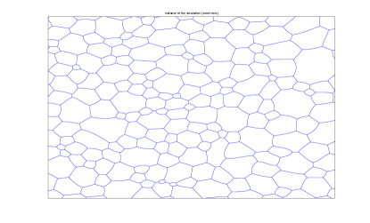
Figure 1. Time instance from the simulation of the 2D grain boundary network with dynamic/time-dependent orientation (zoom view).

Now, for $j=1,2,3$, let $\alpha^{(j)}=\alpha^{(j)}(t)$ be the lattice orientation angle of the grain which is enclosed between grain boundaries $\Gamma_{t}^{(j)}$ and $\Gamma_{t}^{(j+1)}$, and we set that $\Gamma_{t}^{(4)}=\Gamma_{t}^{(1)}$ for the simplicity of the notation. Similar to work [3, 4, 5, 2, 15], we assume here that the orientation $\alpha^{(j)}$ is a bounded scalar since we consider a planar grain boundary network. In this work, we make an assumption that lattice orientations are functions of time $t$ (we assume that during grain growth, grains can change their lattice orientations due to rotation), but independent of the parameter $s$. Next, we define, the surface energy density or interfacial grain boundary energy of $\Gamma_{t}^{(j)}$ as

$$\sigma=\sigma(\bm{n}^{(j)},\alpha^{(j-1)}-\alpha^{(j)})=\sigma(\bm{n}^{(j)},\Delta\alpha^{(j)})\geq 0,$$

where we denote $\Delta\alpha^{(j)}:=\alpha^{(j-1)}-\alpha^{(j)}$ to be misorientation angle across the grain boundary (a common boundary for two neighboring grains with orientations $\alpha^{(j-1)}$ and $\alpha^{(j)}$), and we set for convenience $\alpha^{(0)}:=\alpha^{(3)}$, see Fig. 2. See also Remark 5.5 in Section 5.

The total grain boundary energy of the system $\Gamma_{t}$ can be obtained as

(2.1) $$E(t)=\sum_{j=1}^{3}\int_{\Gamma_{t}^{(j)}}\sigma(\bm{n}^{(j)},\Delta\alpha^{(j)})\,d\mathscr{H}^{1}=\sum_{j=1}^{3}\int_{0}^{1}\sigma(\bm{n}^{(j)},\Delta\alpha^{(j)})|\bm{b}^{(j)}|\,ds,$$

where $\mathscr{H}^{1}$ is the $1$-dimensional Hausdorff measure, (see Fig. 2).

Figure 2. The model of grain boundaries/curves $\Gamma^{(j)}_{t}$ with triple junction $\bm{a}(t)$ and with orientations angles (scalars) $\alpha^{(j)}$.

Next, we use the coordinate $(\bm{n},\theta)\in\mathbb{R}^{2}\times\mathbb{R}$ for the surface energy density $\sigma(\bm{n},\theta)$ and assume that $\sigma$ is taken to be positively homogeneous of degree $0$ in $\bm{n}$. Note, that in general, grain boundaries are identified by lattice misorientation and the orientation of the normal vector to the grain boundary. For simplicity of notations, we denote $\sigma^{(j)}:=\sigma(\bm{n}^{(j)},\Delta\alpha^{(j)})$.

Let us now define grain boundary motion that will result in the dissipation of the total grain boundary energy (2.1). Denote by $\hat{\phantom{n}}$ the normalization operator of vectors, e.g. $\hat{\bm{n}}^{(j)}=\frac{\bm{n}^{(j)}}{|\bm{n}^{(j)}|}$. Then, we can compute the rate of change in energy at time $t$ due to grain boundary motion as follows:

(2.2) $$\begin{split}\frac{d}{dt}E(t)&=\sum_{j=1}^{3}\biggl{(}\int_{0}^{1}\nabla_{\bm{n}}\sigma^{(j)}\cdot\frac{d\bm{n}^{(j)}}{dt}|\bm{b}^{(j)}|\,ds+\int_{0}^{1}\sigma^{(j)}\frac{\bm{b}^{(j)}}{|\bm{b}^{(j)}|}\cdot\frac{d\bm{b}^{(j)}}{dt}\,ds\\ &\quad+\int_{0}^{1}\sigma^{(j)}_{\theta}\frac{d(\Delta\alpha^{(j)}))}{dt}|\bm{b}^{(j)}|\,ds\biggr{)}\\ &=\sum_{j=1}^{3}\biggl{(}\int_{0}^{1}\left(|\bm{b}^{(j)}|\mathstrut^{t}\!R\nabla_{\bm{n}}\sigma^{(j)}+\sigma^{(j)}\hat{\bm{b}}^{(j)}\right)\cdot\frac{d\bm{b}^{(j)}}{dt}\,ds\\ &\quad+\int_{0}^{1}\sigma^{(j)}_{\theta}\frac{d(\Delta\alpha^{(j)}))}{dt}|\bm{b}^{(j)}|\,ds\biggr{)}.\end{split}$$

Next, consider a polar angle $\phi^{(j)}$ and set $\hat{\bm{n}}^{(j)}=(\cos\phi^{(j)},\sin\phi^{(j)})$. Since $\sigma^{(j)}$ is positively homogeneous of degree $0$ in $\bm{n}^{(j)}$, we have

$$\nabla_{\bm{n}}\sigma\cdot\bm{n}=0,\quad\mathstrut^{t}R\nabla_{\bm{n}}\sigma=(\mathstrut{}^{t}R\nabla_{\bm{n}}\sigma\cdot\hat{\bm{n}})\hat{\bm{n}},\quad\sigma^{(j)}_{\phi}\hat{\bm{n}}^{(j)}=|\bm{b}^{(j)}|\mathstrut^{t}\!R\nabla_{\bm{n}}\sigma^{(j)},$$

and, thus, we define the vector $\bm{T}^{(j)}$ known as the line tension or capillary stress vector,

$$\bm{T}^{(j)}:=\sigma^{(j)}_{\phi}\hat{\bm{n}}^{(j)}+\sigma^{(j)}\hat{\bm{b}}^{(j)}=|\bm{b}^{(j)}|\mathstrut^{t}\!R\nabla_{\bm{n}}\sigma^{(j)}+\sigma^{(j)}\hat{\bm{b}}^{(j)}.$$

Now, using the change of variable

$$\frac{d\bm{b}^{(j)}}{dt}=\frac{d}{ds}\frac{d\bm{\xi}^{(j)}}{dt},$$

we can rewrite (2.2) as:

(2.3) $$\begin{split}\frac{d}{dt}E(t)&=\sum_{j=1}^{3}\biggl{(}\int_{0}^{1}\bm{T}^{(j)}\cdot\frac{d}{ds}\frac{d\bm{\xi}^{(j)}}{dt}\,ds+\int_{0}^{1}\sigma^{(j)}_{\theta}\frac{d(\Delta\alpha^{(j)}))}{dt}|\bm{b}^{(j)}|\,ds\biggr{)}\\ &=-\sum_{j=1}^{3}\int_{0}^{1}\bm{T}^{(j)}_{s}\cdot\frac{d\bm{\xi}^{(j)}}{dt}\,ds+\sum_{j=1}^{3}\int_{0}^{1}\sigma^{(j)}_{\theta}\frac{d(\Delta\alpha^{(j)}))}{dt}|\bm{b}^{(j)}|\,ds\\ &\quad-\sum_{j=1}^{3}\bm{T}^{(j)}(0,t)\cdot\frac{d\bm{a}}{dt}(t).\end{split}$$

For the reader’s convenience, we will recall below the following property for a divergence of the capillary stress vector $\bm{T}^{(j)}.$

Lemma 2.1.

Let $\kappa^{(j)}$ is the curvature of $\Gamma_{t}^{(j)}$. Then

(2.4) $$\bm{T}^{(j)}_{s}=|\bm{b}^{(j)}|(\sigma_{\phi\phi}^{(j)}+\sigma^{(j)})\kappa^{(j)}\hat{\bm{n}}^{(j)}.$$

Proof.

From the Frenet-Serret formula for the non-arc length parameter,

(2.5) $$\hat{\bm{b}}_{s}^{(j)}=|\bm{b}^{(j)}|\kappa^{(j)}\hat{\bm{n}}^{(j)},\quad\hat{\bm{n}}_{s}^{(j)}=-|\bm{b}^{(j)}|\kappa^{(j)}\hat{\bm{b}}^{(j)}.$$

Thus we obtain,

(2.6) $$\begin{split}\bm{T}_{s}^{(j)}&=\left(\nabla_{\bm{n}}\sigma^{(j)}_{\phi}\cdot\bm{n}^{(j)}_{s}\right)\hat{\bm{n}}^{(j)}+\sigma^{(j)}_{\phi}\hat{\bm{n}}^{(j)}_{s}+\left(\nabla_{\bm{n}}\sigma^{(j)}\cdot\bm{n}^{(j)}_{s}\right)\hat{\bm{b}}^{(j)}+\sigma^{(j)}\hat{\bm{b}}^{(j)}_{s}\\ &=\left(\mathstrut{}^{t}\!R\nabla_{\bm{n}}\sigma^{(j)}_{\phi}\cdot\bm{b}^{(j)}_{s}+|\bm{b}^{(j)}|\sigma^{(j)}\kappa^{(j)}\right)\hat{\bm{n}}^{(j)}+\left(-|\bm{b}^{(j)}|\sigma^{(j)}_{\phi}\kappa^{(j)}+\mathstrut^{t}\!R\nabla_{\bm{n}}\sigma^{(j)}\cdot\bm{b}^{(j)}_{s}\right)\hat{\bm{b}}^{(j)}.\end{split}$$

Since $\sigma^{(j)}$ and $\sigma_{\phi}^{(j)}$ are positively homogeneous of degree $0$ in $\bm{n}^{(j)}$, we have,

(2.7) $$\sigma^{(j)}_{\phi}\hat{\bm{n}}^{(j)}=|\bm{b}^{(j)}|\mathstrut^{t}\!R\nabla_{\bm{n}}\sigma^{(j)},\quad\sigma^{(j)}_{\phi\phi}\hat{\bm{n}}^{(j)}=|\bm{b}^{(j)}|\mathstrut^{t}\!R\nabla_{\bm{n}}\sigma_{\phi}^{(j)}.$$

Using the orthogonal relation $\bm{b}^{(j)}\cdot\hat{\bm{n}}^{(j)}=0$ and the Frenet-Serret formula (2.5), we obtain,

(2.8) $$\bm{b}_{s}^{(j)}\cdot\hat{\bm{n}}^{(j)}=-\bm{b}^{(j)}\cdot\hat{\bm{n}}^{(j)}_{s}=|\bm{b}^{(j)}|^{2}\kappa^{(j)}.$$

Plugging (2.7) and (2.8) into (2.6), we derive (2.4).

∎

Next, to ensure that the entire system of grain boundaries is dissipative, i.e.

$$\frac{d}{dt}E(t)\leq 0,$$

we impose Mullins theory (curvature driven growth) [29, 30] as the local evolution law stating that the normal velocity $v_{n}^{(j)}$ of a grain boundary of $\Gamma_{t}^{(j)}$ (the rate of growth of area adjacent to the boundary $\Gamma^{(j)}_{t}$), is proportional to the line force $\bm{T}_{s}^{(j)}$ (to the work done through deforming the curve), through the factor of the mobility $\mu^{(j)}>0:$

(2.9) $$v_{n}^{(j)}\hat{\bm{n}}^{(j)}=\mu^{(j)}\frac{1}{|\bm{b}^{(j)}|}\bm{T}_{s}^{(j)}=\mu^{(j)}(\sigma_{\phi\phi}^{(j)}+\sigma^{(j)})\kappa^{(j)}\hat{\bm{n}}^{(j)}\quad\text{on}\ \Gamma_{t}^{(j)},\quad j=1,2,3.$$

Note, that using variation of the energy $E$ with respect to the curve $\bm{\xi}^{(j)}$, namely,

$$v_{n}^{(j)}\hat{\bm{n}}^{(j)}=-\mu^{(j)}\frac{\delta E}{\delta\bm{\xi}^{(j)}},$$

one can derive the following relation for the line force $\bm{T}_{s}^{(j)}$ [20],

(2.10) $$\mu^{(j)}\frac{1}{|\bm{b}^{(j)}|}\bm{T}_{s}^{(j)}=\mu^{(j)}(\sigma_{\phi\phi}^{(j)}+\sigma^{(j)})\kappa^{(j)}\hat{\bm{n}}^{(j)}\quad\text{on}\ \Gamma_{t}^{(j)},\quad j=1,2,3.$$

Since $v_{n}^{(j)}=\frac{d\bm{\xi}^{(j)}}{dt}\cdot\hat{\bm{n}}^{(j)}$, we obtain that,

(2.11) $$\bm{T}^{(j)}_{s}\cdot\frac{d\bm{\xi}^{(j)}}{dt}=\frac{1}{\mu^{(j)}}|v_{n}^{(j)}|^{2}|\bm{b}^{(j)}|\geq 0,$$

and, thus, the first term on the right-hand side of (2.3) is non-positive. Next, we consider the second term on the right-hand side of (2.3) which depends on the derivative of lattice misorientation, we have that (since $\alpha^{(j)}$ is independent of $s$),

$$\sum_{j=1}^{3}\int_{0}^{1}\sigma^{(j)}_{\theta}\frac{d(\Delta\alpha^{(j)}))}{dt}|\bm{b}^{(j)}|\,ds=\sum_{j=1}^{3}\biggl{(}\int_{0}^{1}\Bigl{(}\sigma^{(j+1)}_{\theta}|\bm{b}^{(j+1)}|-\sigma^{(j)}_{\theta}|\bm{b}^{(j)}|\Bigr{)}\,ds\biggr{)}\frac{d\alpha^{(j)}}{dt},$$

where we used that $\sigma^{(4)}=\sigma^{(1)}$. To ensure, $\frac{d}{dt}E(t)\leq 0$ in (2.3), we make an assumption that for a constant $\gamma>0$, we have the following relation for the rate of change of the lattice orientations,

(2.12) $$\frac{d\alpha^{(j)}}{dt}=-\gamma\biggl{(}\int_{0}^{1}\Bigl{(}\sigma^{(j+1)}_{\theta}|\bm{b}^{(j+1)}|-\sigma^{(j)}_{\theta}|\bm{b}^{(j)}|\Bigr{)}\,ds\biggr{)},\quad j=1,2,3$$

since the relation (2.12) results in the condition,

(2.13) $$\sum_{j=1}^{3}\int_{0}^{1}\sigma^{(j)}_{\theta}\frac{d(\Delta\alpha^{(j)}))}{dt}|\bm{b}^{(j)}|\,ds=-\frac{1}{\gamma}\sum_{j=1}^{3}\left|\frac{d\alpha^{(j)}}{dt}\right|^{2}\leq 0$$

on the second term in the right-hand side of (2.3). Note, that the proposed relation (2.12) can also be derived using variation of the energy $E$ with respect to lattice orientation $\alpha^{(j)}$, namely,

$$\frac{d\alpha^{(j)}}{dt}=-\gamma\frac{\delta E}{\delta\alpha^{(j)}}.$$

Remark 2.2.

1. As we discussed, the misorientations are defined using the orientations, $\alpha^{(j)}$ as, $\Delta\alpha^{(j)}=\alpha^{(j-1)}-\alpha^{(j)}$. Conversely, if the sum of the misorientations is zero, namely, $\Delta\alpha^{(1)}+\Delta\alpha^{(2)}+\Delta\alpha^{(3)}=0$, then the following linear relation,

$$\left\{\begin{split}\alpha^{(3)}-\alpha^{(1)}&=\Delta\alpha^{(1)},\\ \alpha^{(1)}-\alpha^{(2)}&=\Delta\alpha^{(2)},\\ \alpha^{(2)}-\alpha^{(3)}&=\Delta\alpha^{(3)}\end{split}\right.$$

can be solved in terms of $\alpha^{(j)}$, and the (inverse) mapping,

$$\begin{pmatrix}\Delta\alpha^{(1)},\ \Delta\alpha^{(2)},\ \Delta\alpha^{(3)}\end{pmatrix}\mapsto\begin{pmatrix}c-\Delta\alpha^{(1)},\ c+\Delta\alpha^{(3)},\ c\end{pmatrix}=\begin{pmatrix}\alpha^{(1)},\ \alpha^{(2)},\ \alpha^{(3)}\end{pmatrix}$$

gives the orientations from the misorientations $\Delta\alpha^{(j)}$. Here $c$ is an arbitrary parameter. Thus, if we would formulate/derive equations for the misorientation evolution, instead of the equation for the orientation (2.12), we would have to impose additional constraint, $(\Delta\alpha^{(1)}+\Delta\alpha^{(2)}+\Delta\alpha^{(3)})(0)=0$. Furthermore, in that case, the orientation of each grain may not be determined uniquely due to the arbitrary parameter $c$. On the other hand, from (2.12) it follows directly that,

$$\frac{d}{dt}(\alpha^{(1)}+\alpha^{(2)}+\alpha^{(3)})=0.$$

Hence, the sum of the orientations $\alpha^{(1)}+\alpha^{(2)}+\alpha^{(3)}$ has to be a constant. This constraint for the orientations is easily determined by the initial configuration, and both the orientations and the misorientations can be determined from the equation (2.12).
2. As discussed above, in our work, we consider the orientation as the primary variable, and we enforce dissipation in the system by assuming relation (2.12) through the orientation. Note that, we consider the rate of the change on the orientation (rather than on the misorientation) since we study system before critical events/disappearance events. Moreover, this choice of the orientation as the primary variable is also consistent with a case of grain boundary energy $\sigma(\bm{n}^{(j)},\Delta\alpha^{(j)})$. In addition, note that, the traditional texture distribution is the orientation distribution. However, in general, one can obtain the misorientation distribution, by considering the convolution of the orientation distribution with itself, or see the above remark.

We also note that (2.12) is not a unique way to ensure dissipative system, and other relations for the rate of change of the lattice orientations which enforce dissipation may be possible. In this work, the particular assumption on the rate of change of the lattice orientation (2.12) is motivated by the approximation to the gradient flow dynamics near equilibrium [4, 2]. Experimental study of the dynamics of the lattice orientations/misorientations will be part of future research.

Finally, as a part of $\frac{d}{dt}E(t)\leq 0$ condition in (2.3), we also assume the dynamic boundary conditions for the triple junctions, namely, for a constant $\eta>0$,

(2.14) $$\frac{d\bm{a}}{dt}(t)=\eta\sum_{j=1}^{3}\bm{T}^{(j)}(0,t),\quad t>0.$$

This assumption implies that the last term in (2.3) satisfies,

(2.15) $$-\sum_{j=1}^{3}\bm{T}^{(j)}(0,t)\cdot\frac{d\bm{a}}{dt}(t)=-\frac{1}{\eta}\left|\frac{d\bm{a}}{dt}(t)\right|^{2}\leq 0.$$

Therefore, we obtain from (2.11), (2.13), and (2.15), that the entire system of grain boundaries $\Gamma_{t}^{(j)}$ is dissipative, namely,

(2.16) $$\frac{d}{dt}E(t)=-\sum_{j=1}^{3}\int_{\Gamma_{t}^{(j)}}\frac{1}{\mu^{(j)}}|v_{n}^{(j)}|^{2}\,d\mathscr{H}^{1}-\frac{1}{\eta}\left|\frac{d\bm{a}}{dt}(t)\right|^{2}-\frac{1}{\gamma}\sum_{j=1}^{3}\left|\frac{d\alpha^{(j)}}{dt}\right|^{2}\leq 0.$$

Finally, we combine assumptions (2.9), (2.12), and (2.14) to obtain the following system of geometric evolution differential equations to describe motion of grain boundaries $\Gamma^{(j)}_{t},j=1,2,3$ together with a motion of the triple junction $\bm{a}(t)$:

(2.17) $$\left\{\begin{aligned} v_{n}^{(j)}&=\mu^{(j)}(\sigma^{(j)}_{\phi\phi}+\sigma^{(j)})\kappa^{(j)},\quad\text{on}\ \Gamma_{t}^{(j)},\ t>0,\quad j=1,2,3,\\ \frac{d\alpha^{(j)}}{dt}&=-\gamma\biggl{(}\int_{0}^{1}\Bigl{(}\sigma^{(j+1)}_{\theta}|\bm{b}^{(j+1)}|-\sigma^{(j)}_{\theta}|\bm{b}^{(j)}|\Bigr{)}\,ds\biggr{)},\quad j=1,2,3,\\ \frac{d\bm{a}}{dt}(t)&=\eta\sum_{k=1}^{3}\bm{T}^{(k)}(0,t)=\eta\sum_{k=1}^{3}(\sigma_{\phi}^{(k)}\hat{\bm{n}}^{(k)}+\sigma^{(k)}\hat{\bm{b}}^{(k)})(0,t),\quad t>0,\\ \Gamma_{t}^{(j)}&:\bm{\xi}^{(j)}(s,t),\quad 0\leq s\leq 1,\quad t>0,\quad j=1,2,3,\\ \bm{a}(t)&=\bm{\xi}^{(1)}(0,t)=\bm{\xi}^{(2)}(0,t)=\bm{\xi}^{(3)}(0,t),\quad\text{and}\quad\bm{\xi}^{(j)}(1,t)=\bm{x}^{(j)},\quad j=1,2,3.\end{aligned}\right.$$

Remark 2.3.

The entire system (2.17) satisfies energy dissipation principle (2.16). However, it is important to note, that there are three independent relaxation time scales in the system (2.17), namely, $\mu^{(j)},\gamma$ and $\eta$ (length, misorientation and position of the triple junction). Classical approach is to let $\gamma\rightarrow\infty$ and $\eta\rightarrow\infty$.

In this work, we let $\mu^{(j)}\rightarrow\infty$, and set $\gamma=\eta=1$ to study the effect of the dynamics of lattice orientations $\alpha^{(j)}(t),j=1,2,3$ together with the effect of the dynamics of a triple junction $\bm{a}(t)$ on a grain boundary motion. Then, in this limit, $\Gamma^{(j)}_{t}$ becomes a line segment from the triple junction $\bm{a}(t)$ to the boundary point $\bm{x}^{(j)}$. Hence, we have

$$\left\{\begin{aligned} \bm{\xi}^{(j)}(s,t)&=\bm{a}(t)+s\bm{b}^{(j)}(t),\quad 0\leq s\leq 1,\quad t>0,\quad j=1,2,3,\\ \bm{a}(t)+\bm{b}^{(j)}(t)&=\bm{x}^{(j)},\quad j=1,2,3.\end{aligned}\right.$$

We assume that the surface tension $\sigma$ is independent of the normal vector $\bm{n}$. Hereafter, we further assume the following three conditions for the surface tension $\sigma$. First, we assume positivity, namely, there exists a positive constant $\Cl{const:2.Assumption1}>0$ such that,

(2.18) $$\sigma(\theta)\geq\Cr{const:2.Assumption1},$$

for $\theta\in\mathbb{R}$. Second, we assume convexity, for all $\theta\in\mathbb{R},$

(2.19) $$\sigma_{\theta}(\theta)\theta\geq 0.$$

Furthermore, we assume,

(2.20) $$\sigma_{\theta}(\theta)=0\ \text{if and only if}\ \theta=0.$$

Remark 2.4.

1. In this work we assume a more general surface energy $\sigma(\Delta\alpha^{(j)})$ (2.18), (2.20), since we consider a non-equilibrium state at time scale $\mu^{(j)}\rightarrow\infty$ and $\gamma=\eta=1$. Note that a different example of Read-Shockley type surface energy [31] is the classical example of the grain boundary energy derived under the assumption of small misorientation angle $\Delta\alpha^{(j)}$, and the assumption of the equilibrium state for a single fixed grain boundary at time scale $\mu^{(j)}\rightarrow\infty,\eta\rightarrow\infty$ and $\gamma=0$.
2. In this work, for simplicity we consider cases of surface tensions without normal dependence. This assumption is not as restrictive since our model is in terms of the orientation, instead of misorientation, as we had discussed in Remark 2.2. Note also, that the convexity condition (2.19) is not needed for local existence results and dissipation estimates for the energy, Sections 4 -5 and Section 7. The condition (2.19) is essentially used to show the misorientation/orientation estimates, see Sections 3, 5 and 7, and, as a part of future work, we will investigate possibility of relaxing this assumption to derive similar estimates. In addition, in this work, to show uniqueness of the solution to (4.1), we proceed using misorientation/orientation estimates from Section 5. However, one can obtain uniqueness result without the use of those estimates, and instead using the estimate (4.21), in proof of Theorem 4.1.

Thus, the system of geometric evolution differential equations (2.17) becomes the following system of ordinary differential equations (ODE):

(2.21) $$\left\{\begin{aligned} \frac{d\alpha^{(j)}}{dt}&=-\Bigl{(}\sigma_{\theta}(\Delta\alpha^{(j+1)})|\bm{b}^{(j+1)}|-\sigma_{\theta}(\Delta\alpha^{(j)})|\bm{b}^{(j)}|\Bigr{)},\quad j=1,2,3,\\ \frac{d\bm{a}}{dt}(t)&=\sum_{j=1}^{3}\sigma(\Delta\alpha^{(j)})\frac{\bm{b}^{(j)}}{|\bm{b}^{(j)}|},\quad t>0,\\ \bm{a}(t)+\bm{b}^{(j)}(t)&=\bm{x}^{(j)},\quad j=1,2,3.\end{aligned}\right.$$

Below, we continue with a study of the local well-posedness of the problem (2.21) with the initial data given by $\alpha^{(1)}_{0},\alpha^{(2)}_{0},\alpha^{(3)}_{0},\bm{a}_{0}$.

Remark 2.5.

1. Note, that the reduced model (2.21) is not a standard ODE system. This is the ODE system where each variable is locally constrained. Moreover, local well-posedness result (e.g. local existence result) for the original model (2.17) will not imply local well-posedness result for the reduced system (2.21) (it is unknown if the reduced model (2.21) is actually a small perturbation of (2.17).).
2. The reduced model (2.21) captures the dynamics of the orientations/misorientations and the triple junctions, and at the same time is more accessible for the analysis than the model (2.17). In addition, the system (2.21) is consistent/motivated by the model in [4, 5]. The well-posedness analysis of (2.21) is a step towards similar analysis for the model in [4, 5], as well as for the original system (2.17).

3. Equilibrium

We study an associated equilibrium solution of the system (2.21), namely,

(3.1) $$\left\{\begin{aligned} 0&=\Bigl{(}\sigma_{\theta}(\Delta\alpha_{\infty}^{(j+1)})|\bm{b}_{\infty}^{(j+1)}|-\sigma_{\theta}(\Delta\alpha_{\infty}^{(j)})|\bm{b}_{\infty}^{(j)}|\Bigr{)},\\ \bm{0}&=\sum_{j=1}^{3}\left(\sigma(\Delta\alpha_{\infty}^{(j)})\right)\frac{\bm{b}_{\infty}^{(j)}}{|\bm{b}_{\infty}^{(j)}|},\\ \bm{a}_{\infty}+\bm{b}^{(j)}_{\infty}&=\bm{x}^{(j)},\quad j=1,2,3.\end{aligned}\right.$$

To consider the equilibrium system (3.1), we assume that each Dirichlet point $\bm{x}^{(j)}$ does not coincide with the other Dirichlet point.

Lemma 3.1.

Let $(\alpha_{\infty}^{(1)},\alpha_{\infty}^{(2)},\alpha_{\infty}^{(3)},\bm{a}_{\infty})$ be a solution of the equilibrium system (3.1). Assume (2.19) and (2.20). Then $\alpha_{\infty}^{(1)}=\alpha_{\infty}^{(2)}=\alpha_{\infty}^{(3)}$.

Proof.

We multiply the first equation of (3.1) by $\alpha_{\infty}^{(j)}$ and sum to $j=1,2,3$, to obtain

(3.2) $$0=\sum_{j=1}^{3}\Bigl{(}\sigma_{\theta}(\Delta\alpha_{\infty}^{(j+1)})|\bm{b}_{\infty}^{(j+1)}|-\sigma_{\theta}(\Delta\alpha_{\infty}^{(j)})|\bm{b}_{\infty}^{(j)}|\Bigr{)}\alpha^{(j)}_{\infty}=\sum_{j=1}^{3}\Bigl{(}\sigma_{\theta}(\Delta\alpha_{\infty}^{(j)})|\bm{b}_{\infty}^{(j)}|\Bigr{)}\Delta\alpha^{(j)}_{\infty}.$$

Note that, at least two of the terms $|\bm{b}_{\infty}^{(j)}|,j=1,2,3$ are non zero, otherwise it will contradict the assumption that the Dirichlet points $\bm{x}^{(j)}$ are distinct. Hence, from (2.19)-(2.20), we obtain that $\alpha_{\infty}^{(1)}=\alpha_{\infty}^{(2)}=\alpha_{\infty}^{(3)}$. ∎

From Lemma 3.1, it follows that, in the equilibrium state, there is no lattice misorientation between neighboring grains that have grain boundaries meeting at that triple junction. As a consequence, the equilibrium system (3.1) becomes,

(3.3) $$\left\{\begin{aligned} \bm{0}&=\sum_{j=1}^{3}\frac{\bm{b}_{\infty}^{(j)}}{|\bm{b}_{\infty}^{(j)}|},\\ \bm{a}_{\infty}+\bm{b}^{(j)}_{\infty}&=\bm{x}^{(j)},\quad j=1,2,3.\end{aligned}\right.$$

The equation (3.3) is related to the Fermat-Torricelli problem. More precisely, if we have that, for each $i=1,2,3$,

(3.4) $$\left|\sum_{j=1,\ i\neq j}^{3}\frac{\bm{x}^{(j)}-\bm{x}^{(i)}}{|\bm{x}^{(j)}-\bm{x}^{(i)}|}\right|>1,$$

then $\bm{a}_{\infty}$ is the unique minimizer of the function,

(3.5) $$f(\bm{a})=\sum_{j=1}^{3}|\bm{a}-\bm{x}^{(j)}|,\quad\bm{a}\in\mathbb{R}^{2},$$

and $\bm{a}_{\infty}\neq\bm{x}^{(j)}$ for $j=1,2,3$ (See [7, Theorem 18.28]). Note, that the assumption (3.4) satisfies if and only if all three angles of the triangle, formed by vertices located at the nodes $\bm{x}^{(1)}$, $\bm{x}^{(2)}$, $\bm{x}^{(3)}$, are less than $120^{\circ}$.

4. Local existence

Here, we discuss local existence which validates the consistency of the proposed model. Let $\bm{x}^{(j)}\in\mathbb{R}^{2}$, $\bm{\alpha}_{0}=(\alpha_{0}^{(1)},\alpha_{0}^{(2)},\alpha_{0}^{(3)})\in\mathbb{R}^{3}$, and $\bm{a}_{0}\in\mathbb{R}^{2}$ be given initial data and we consider the local existence of the problem of (2.21), namely

(4.1) $$\left\{\begin{aligned} \frac{d\alpha^{(j)}}{dt}&=-\Bigl{(}\sigma_{\theta}(\Delta\alpha^{(j+1)})|\bm{b}^{(j+1)}|-\sigma_{\theta}(\Delta\alpha^{(j)})|\bm{b}^{(j)}|\Bigr{)},\quad j=1,2,3,\\ \frac{d\bm{a}}{dt}(t)&=\sum_{j=1}^{3}\sigma(\Delta\alpha^{(j)})\frac{\bm{b}^{(j)}}{|\bm{b}^{(j)}|},\quad t>0,\\ \bm{\alpha}(t)&=(\alpha^{(1)}(t),\alpha^{(2)}(t),\alpha^{(3)}(t)),\quad t>0,\\ \bm{a}(t)+\bm{b}^{(j)}(t)&=\bm{x}^{(j)},\quad t>0,\quad j=1,2,3,\\ \bm{\alpha}(0)&=\bm{\alpha}_{0},\quad\bm{a}(0)=\bm{a}_{0}.\end{aligned}\right.$$

Assume for each $i=1,2,3$,

(4.2) $$\left|\sum_{j=1,\ i\neq j.}^{3}\frac{\bm{x}^{(j)}-\bm{x}^{(i)}}{|\bm{x}^{(j)}-\bm{x}^{(i)}|}\right|>1.$$

We denote by $\bm{a}_{\infty}\neq\bm{x}^{(j)}$ for each $j=1,2,3$, a solution to the system,

(4.3) $$\left\{\begin{aligned} \bm{0}&=\sum_{j=1}^{3}\frac{\bm{b}_{\infty}^{(j)}}{|\bm{b}_{\infty}^{(j)}|},\\ \bm{a}_{\infty}+\bm{b}^{(j)}_{\infty}&=\bm{x}^{(j)},\quad j=1,2,3.\end{aligned}\right.$$

The point $\bm{a}_{\infty}$ is a triple junction point (see Section 3).

Theorem 4.1 (Local existence).

Let $\bm{x}^{(1)}$, $\bm{x}^{(2)}$, $\bm{x}^{(3)}\in\mathbb{R}^{2}$, $\bm{a}_{0}\in\mathbb{R}^{2}$, and $\bm{\alpha}_{0}\in\mathbb{R}^{3}$ be given initial data. Assume condition (4.2) for $i=1,2,3$, and let $\bm{a}_{\infty}$ be a solution of (4.3). Further, assume that for all $j=1,2,3$,

(4.4) $$|\bm{a}_{0}-\bm{a}_{\infty}|<\frac{1}{2}|\bm{b}^{(j)}_{\infty}|.$$

Then, there exists a local in time solution $(\bm{\alpha},\bm{a})$ of (4.1) on $[0,T_{\text{max}})$, such that

(4.5) $$|\bm{a}(t)-\bm{a}_{\infty}|<|\bm{b}^{(j)}_{\infty}|\quad\text{for all}\quad j=1,2,3,\ \text{and}\ 0\leq t<T_{\text{max}}.$$

Furthermore, the maximal existence time $T_{\text{max}}$ of the solution is estimated by

(4.6) $$T_{\text{max}}\geq\min\left\{\frac{|\bm{\alpha}_{0}|}{4(M_{1}+8M_{2}|\bm{\alpha}_{0}|)\sum_{j=1}^{3}|\bm{b}^{(j)}_{\infty}|},\ \frac{|\bm{a}_{0}-\bm{a}_{\infty}|}{3M_{0}},\ \frac{1}{12M_{1}},\ \frac{1}{8M_{0}\sum_{j=1}^{3}\frac{1}{|\bm{b}_{\infty}^{(j)}|-2|\bm{a}_{0}-\bm{a}_{\infty}|}}\right\},$$

where

$$M_{0}:=\sup_{|\theta|\leq 4|\bm{\alpha}_{0}|}|\sigma(\theta)|,\quad M_{1}:=\sup_{|\theta|\leq 4|\bm{\alpha}_{0}|}|\sigma_{\theta}(\theta)|,\quad M_{2}:=\sup_{|\theta_{1}|,|\theta_{2}|\leq 4|\bm{\alpha}_{0}|}\frac{|\sigma_{\theta}(\theta_{1})-\sigma_{\theta}(\theta_{2})|}{|\theta_{1}-\theta_{2}|}.$$

Remark 4.2.

The Theorem 4.1 provides not only existence of the local in time solution for the model (4.1), but it also gives the local existence of the triple junction. The estimate (4.5) guarantees that $\bm{a}(t)$ is the position of the triple junction formed by the grain boundaries $\bm{x}^{(j)}-\bm{a}(t)$. Note, if $\bm{a}(t)$ is sufficiently far from the position of the triple junction $\bm{a}_{\infty}$ of the equilibrium state, for instance if $\bm{x}^{(j)}-\bm{x}^{(k)}$ is a part of $\bm{a}(t)-\bm{x}^{(k)}$, then $\bm{a}(t)$ might not be the triple junction. Further, (4.6) gives the explicit dependence of the maximal existence time $T_{\text{max}}$ on $|\bm{a}_{0}-\bm{a}_{\infty}|$. This is an important result for the analysis of the global in time solution which will be part of a forthcoming work.

To show Theorem 4.1, we construct a contraction mapping on a complete metric space. Let $\Cl{const:4.1}$, $\Cl{const:4.2}>0$ and $T>0$ be positive constants that we will define later, and denote,

$$X_{T}:=\{(\bm{\alpha},\bm{a})\in C([0,T]\,;\,\mathbb{R}^{3}\times\mathbb{R}^{2}),\ \|\bm{\alpha}\|_{C([0,T])}\leq\Cr{const:4.1},\ \|\bm{a}-\bm{a}_{\infty}\|_{C([0,T])}\leq\Cr{const:4.2}\}.$$

Note that in the definition of the space $X_{T}$, we use the position of the triple junction $\bm{a}_{\infty}$ at the equilibrium state as the point of reference, rather than the position of the triple junction $\bm{a}_{0}$ at the initial time as one would consider in the classical ODE theory. Such definition of the space $X_{T}$ is employed in order to obtain the estimates on the position of the triple junctions from the one of the equilibrium state $\bm{a}_{\infty}$, (4.5), as well as to derive the maximal existence time estimate (4.6).

Next, define for $(\bm{\alpha},\bm{a})\in X_{T}$, $i=1,2,3$, and $t>0$

(4.7) $$\begin{split}\Phi^{(i)}(\bm{\alpha},\bm{a})(t)&:=\alpha^{(i)}_{0}-\int_{0}^{t}\left(\sigma_{\theta}(\Delta\alpha^{(j+1)}(\tau))|\bm{b}^{(j+1)}(\tau)|-\sigma_{\theta}(\Delta\alpha^{(j)}(\tau))|\bm{b}^{(j)}(\tau)|\right)\,d\tau,\\ \Psi(\bm{\alpha},\bm{a})(t)&:=\bm{a}_{0}+\sum_{j=1}^{3}\int_{0}^{t}\sigma(\alpha(\tau))\frac{\bm{b}^{(j)}(\tau)}{|\bm{b}^{(j)}(\tau)|}\,d\tau,\end{split}$$

where $\bm{b}^{(j)}(\tau)=\bm{x}^{(j)}-\bm{a}(\tau)$. Our goal now is to show that $(\Phi=(\Phi^{(1)},\Phi^{(2)},\Phi^{(3)}),\Psi)$ is a contraction mapping on $X_{T}$ for the appropriate choice of positive constants $\Cr{const:4.1}$, $\Cr{const:4.2}$, and $T>0$. Hereafter we define,

$$M_{0}:=\sup_{|\theta|\leq 2C_{2}}|\sigma(\theta)|,\quad M_{1}:=\sup_{|\theta|\leq 2C_{2}}|\sigma_{\theta}(\theta)|,\quad M_{2}:=\sup_{|\theta_{1}|,|\theta_{2}|\leq 2\Cr{const:4.1}}\frac{|\sigma_{\theta}(\theta_{1})-\sigma_{\theta}(\theta_{2})|}{|\theta_{1}-\theta_{2}|}.$$

Later, the constant $\Cr{const:4.1}$ will be taken to be $2|\bm{\alpha}_{0}|$. Next, two Lemmas 4.3, 4.4 show that $\Phi$ and $\Psi$ is a map on $X_{T}$.

Lemma 4.3.

If the conditions below are satisfied,

(4.8) $$2|\bm{\alpha}_{0}|\leq\Cr{const:4.1},$$

and

(4.9) $$(2M_{1}+4M_{2}\Cr{const:4.1})(|\bm{b}^{(1)}_{\infty}|+|\bm{b}^{(2)}_{\infty}|+|\bm{b}^{(3)}_{\infty}|+3\Cr{const:4.2})T\leq\frac{1}{2}\Cr{const:4.1},$$

then $|\Phi(\bm{\alpha},\bm{a})|\leq\Cr{const:4.1}$ for all $(\bm{\alpha},\bm{a})\in X_{T}$.

Proof of Lemma 4.3.

By the triangle inequality, for $0\leq t\leq T$,

$$\begin{split}|\Phi(\bm{\alpha},\bm{a})(t)|&\leq|\bm{\alpha}_{0}|+\sum_{j=1}^{3}\left|\int_{0}^{t}\left(\sigma_{\theta}(\Delta\alpha^{(j+1)}(\tau))|\bm{b}^{(j+1)}(\tau)|-\sigma_{\theta}(\Delta\alpha^{(j)}(\tau))|\bm{b}^{(j)}(\tau)|\right)\,d\tau\right|\\ &\leq|\bm{\alpha}_{0}|+\sum_{j=1}^{3}\bigg{(}\int_{0}^{t}|\sigma_{\theta}(\Delta\alpha^{(j+1)}(\tau))-\sigma_{\theta}(\Delta\alpha^{(j)}(\tau))||\bm{b}^{(j+1)}(\tau)|\,d\tau\\ &\quad+\int_{0}^{t}|\sigma_{\theta}(\Delta\alpha^{(j)}(\tau))|\left||\bm{b}^{(j+1)}(\tau)|-|\bm{b}^{(j)}(\tau)|\right|\,d\tau\bigg{)}.\end{split}$$

Next, using that $|\Delta\alpha^{(j)}|\leq 2\Cr{const:4.1}$, and that,

$$|\sigma_{\theta}(\Delta\alpha^{(j+1)}(\tau))-\sigma_{\theta}(\Delta\alpha^{(j)}(\tau))|\leq M_{2}|\Delta\alpha^{(j+1)}(\tau)-\Delta\alpha^{(j)}(\tau)|\leq 4M_{2}\Cr{const:4.1},$$

we have that,

$$|\Phi(\bm{\alpha},\bm{a})(t)|\leq|\bm{\alpha}_{0}|+(2M_{1}+4M_{2}\Cr{const:4.1})T\sum_{j=1}^{3}\sup_{0\leq\tau\leq T}|\bm{b}^{(j)}(\tau)|.$$

On the other hand, for $j=1,2,3$,

(4.10) $$|\bm{b}^{(j)}(t)|=|\bm{x}^{(j)}-\bm{a}_{\infty}+\bm{a}_{\infty}-\bm{a}(t)|\leq|\bm{b}^{(j)}_{\infty}|+\Cr{const:4.2}.$$

Therefore, from (4.8) and (4.9),

$$|\Phi(\bm{\alpha},\bm{a})(t)|\leq|\bm{\alpha}_{0}|+(2M_{1}+4M_{2}\Cr{const:4.1})(|\bm{b}^{(1)}_{\infty}|+|\bm{b}^{(2)}_{\infty}|+|\bm{b}^{(3)}_{\infty}|+3\Cr{const:4.2})T\leq\Cr{const:4.1}.$$

∎

Lemma 4.4.

Assume for $j=1,2,3$ we have that,

(4.11) $$\Cr{const:4.2}<|\bm{b}_{\infty}^{(j)}|.$$

Then, $0<|\bm{b}_{\infty}^{(j)}|-\Cr{const:4.2}\leq|\bm{b}^{(j)}(t)|\leq|\bm{b}^{(j)}_{\infty}|+\Cr{const:4.2},$ for all $j=1,2,3$, $(\bm{\alpha},\bm{a})\in X_{T}$, and $0\leq t\leq T$. Further if

(4.12) $$2|\bm{a}_{0}-\bm{a}_{\infty}|\leq\Cr{const:4.2},$$

and

(4.13) $$3M_{0}T\leq\frac{1}{2}\Cr{const:4.2},$$

then $|\Psi(\bm{\alpha},\bm{a})(t)-\bm{a}_{\infty}|\leq\Cr{const:4.2},$ for all $(\bm{\alpha},\bm{a})\in X_{T}$ and $0\leq t\leq T$.

Proof of Lemma 4.4.

For $(\bm{\alpha},\bm{a})\in X_{T}$, and $0\leq t\leq T$

$$|\bm{b}_{\infty}^{(j)}|=|\bm{x}^{(j)}-\bm{a}(t)+\bm{a}(t)-\bm{a}_{\infty}|\leq|\bm{b}^{(j)}(t)|+|\bm{a}(t)-\bm{a}_{\infty}|\leq|\bm{b}^{(j)}(t)|+\Cr{const:4.2},$$

thus we obtain $0<|\bm{b}_{\infty}^{(j)}|-\Cr{const:4.2}\leq|\bm{b}^{(j)}(t)|$. And $|\bm{b}^{(j)}(t)|\leq|\bm{b}^{(j)}_{\infty}|+\Cr{const:4.2}$ follows from (4.10). To show estimate $|\Psi(\bm{\alpha},\bm{a})(t)-\bm{a}_{\infty}|\leq\Cr{const:4.2}$, we use the assumption (4.12) and (4.13), to obtain that for any $(\bm{\alpha},\bm{a})\in X_{T}$,

$$\begin{split}|\Psi(\bm{\alpha},\bm{a})(t)-\bm{a}_{\infty}|&\leq|\bm{a}_{0}-\bm{a}_{\infty}|+\sum_{j=1}^{3}\left|\int_{0}^{t}\sigma(\Delta\alpha^{(j)}(\tau))\frac{\bm{b}^{(j)}(\tau)}{|\bm{b}^{(j)}(\tau)|}\,d\tau\right|\\ &\leq\frac{1}{2}\Cr{const:4.2}+\sum_{j=1}^{3}\sup_{0\leq\tau\leq T}\sigma(\Delta\alpha^{(j)}(\tau))T\\ &\leq\frac{1}{2}\Cr{const:4.2}+3M_{0}T\leq\Cr{const:4.2},\end{split}$$

for all $0\leq t\leq T$. ∎

The next two Lemmas 4.5 and 4.6 give the Lipschitz property of the map $(\Phi,\Psi)$.

Lemma 4.5 (Lipschitz estimates).

For $(\bm{\alpha}_{1},\bm{a}_{1})$, $(\bm{\alpha}_{2},\bm{a}_{2})\in X_{T}$, we have that

(4.14) $$\begin{split}&\quad\|\Phi(\bm{\alpha}_{1},\bm{a}_{1})-\Phi(\bm{\alpha}_{2},\bm{a}_{2})\|_{C([0,T])}\\ &\leq 4M_{2}(|\bm{b}_{\infty}^{(1)}|+|\bm{b}_{\infty}^{(2)}|+|\bm{b}_{\infty}^{(3)}|+3\Cr{const:4.2})T\|\bm{\alpha}_{1}-\bm{\alpha}_{2}\|_{C([0,T])}+6M_{1}T\|\bm{a}_{1}-\bm{a}_{2}\|_{C([0,T])}.\end{split}$$

Proof of Lemma 4.5.

For $0\leq t\leq T$, by the Lipschitz continuity of $\sigma_{\theta}$ we obtain that

$$\begin{split}&\quad|\Phi(\bm{\alpha}_{1},\bm{a}_{1})(t)-\Phi(\bm{\alpha}_{2},\bm{a}_{2})(t)|\\ &\leq\sum_{j=1}^{3}\left|\int_{0}^{t}\left(\sigma_{\theta}(\Delta\alpha^{(j+1)}_{1})|\bm{b}^{(j+1)}_{1}|-\sigma_{\theta}(\Delta\alpha^{(j)}_{1})|\bm{b}^{(j)}_{1}|-\sigma_{\theta}(\Delta\alpha^{(j+1)}_{2})|\bm{b}^{(j+1)}_{2}|+\sigma_{\theta}(\Delta\alpha^{(j)}_{2})|\bm{b}^{(j)}_{2}|\right)\,d\tau\right|\\ &\leq\sum_{j=1}^{3}\int_{0}^{t}\left(\left|\sigma_{\theta}(\Delta\alpha^{(j+1)}_{1})\right|\left||\bm{b}^{(j+1)}_{1}|-|\bm{b}^{(j+1)}_{2}|\right|+\left|\sigma_{\theta}(\Delta\alpha^{(j+1)}_{1})-\sigma_{\theta}(\Delta\alpha^{(j+1)}_{2})\right||\bm{b}^{(j+1)}_{2}|\right)\,d\tau\\ &\quad+\sum_{j=1}^{3}\int_{0}^{t}\left(\left|\sigma_{\theta}(\Delta\alpha^{(j)}_{1})\right|\left||\bm{b}^{(j)}_{1}|-|\bm{b}^{(j)}_{2}|\right|+\left|\sigma_{\theta}(\Delta\alpha^{(j)}_{1})-\sigma_{\theta}(\Delta\alpha^{(j)}_{2})\right||\bm{b}^{(j)}_{2}|\right)\,d\tau.\end{split}$$

Next, using $\bm{b}^{(j)}_{k}=\bm{x}^{(j)}-\bm{a}_{k},$ $\Delta\alpha^{(j)}=\alpha^{(j-1)}-\alpha^{(j)}$ and (4.10), we have,

$$|\Phi(\bm{\alpha}_{1},\bm{a}_{1})(t)-\Phi(\bm{\alpha}_{2},\bm{a}_{2})(t)|\leq 6M_{1}T\|\bm{a}_{1}-\bm{a}_{2}\|_{C([0,T])}+4M_{2}(|\bm{b}_{\infty}^{(1)}|+|\bm{b}_{\infty}^{(2)}|+|\bm{b}_{\infty}^{(3)}|+3\Cr{const:4.2})T\|\bm{\alpha}_{1}-\bm{\alpha}_{2}\|_{C([0,T])}.$$

Thus, we obtain the inequality (4.14).

∎

Lemma 4.6 (Lipschitz estimates).

Assume condition (4.11) holds true. Then for $(\bm{\alpha}_{1},\bm{a}_{1})$, $(\bm{\alpha}_{2},\bm{a}_{2})\in X_{T}$, we have that

(4.15) $$\begin{split}&\quad\|\Psi(\bm{\alpha}_{1},\bm{a}_{1})(t)-\Psi(\bm{\alpha}_{2},\bm{a}_{2})(t)\|_{C([0,T])}\\ &\leq 6M_{1}T\|\bm{\alpha}_{1}-\bm{\alpha}_{2}\|_{C([0,T])}+2M_{0}\left(\frac{1}{|\bm{b}_{\infty}^{(1)}|-\Cr{const:4.2}}+\frac{1}{|\bm{b}_{\infty}^{(2)}|-\Cr{const:4.2}}+\frac{1}{|\bm{b}_{\infty}^{(3)}|-\Cr{const:4.2}}\right)T\|\bm{a}_{1}-\bm{a}_{2}\|_{C([0,T])}.\end{split}$$

Proof of Lemma 4.6.

For $k=1,2$, denote $\sigma^{(j)}_{k}(t):=\sigma(\Delta\alpha^{(j)}_{k}(t))$. For $0\leq t\leq T$, we can obtain the following estimate

$$\begin{split}|\Psi(\bm{\alpha}_{1},\bm{a}_{1})(t)-\Psi(\bm{\alpha}_{2},\bm{a}_{2})(t)|&=\left|\sum_{j=1}^{3}\int_{0}^{t}\left(\sigma^{(j)}_{1}(\tau)\frac{\bm{b}_{1}^{(j)}(\tau)}{|\bm{b}_{1}^{(j)}(\tau)|}-\sigma^{(j)}_{2}(\tau)\frac{\bm{b}_{2}^{(j)}(\tau)}{|\bm{b}_{2}^{(j)}(\tau)|}\right)\,d\tau\right|\\ &\leq\sum_{j=1}^{3}\int_{0}^{T}\left|\sigma^{(j)}_{1}(\tau)\frac{\bm{b}_{1}^{(j)}(\tau)}{|\bm{b}_{1}^{(j)}(\tau)|}-\sigma^{(j)}_{2}(\tau)\frac{\bm{b}_{2}^{(j)}(\tau)}{|\bm{b}_{2}^{(j)}(\tau)|}\right|\,d\tau\\ &\leq\sum_{j=1}^{3}\int_{0}^{T}\left|\sigma^{(j)}_{1}(\tau)-\sigma^{(j)}_{2}(\tau)\right|\,d\tau\\ &\quad+\sum_{j=1}^{3}\int_{0}^{T}\sigma^{(j)}_{2}(\tau)\left|\frac{\bm{b}_{1}^{(j)}(\tau)}{|\bm{b}_{1}^{(j)}(\tau)|}-\frac{\bm{b}_{2}^{(j)}(\tau)}{|\bm{b}_{2}^{(j)}(\tau)|}\right|\,d\tau.\end{split}$$

Since $(\bm{\alpha}_{k},\bm{a}_{k})\in X_{T}$, we have

$$\begin{split}\left|\sigma^{(j)}_{1}(\tau)-\sigma^{(j)}_{2}(\tau)\right|&=|\sigma(\Delta\alpha_{1}^{(j)}(\tau))-\sigma(\Delta\alpha_{2}^{(j)}(\tau))|\\ &\leq M_{1}|\Delta\alpha_{1}^{(j)}(\tau)-\Delta\alpha_{2}^{(j)}(\tau)|\\ &\leq 2M_{1}\|\bm{\alpha}_{1}-\bm{\alpha}_{2}\|_{C([0,T])}.\end{split}$$

Hence, we derive that

$$\sum_{j=1}^{3}\int_{0}^{T}\left|\sigma^{(j)}_{1}(\tau)-\sigma^{(j)}_{2}(\tau)\right|\,d\tau\leq 6M_{1}T\|\bm{\alpha}_{1}-\bm{\alpha}_{2}\|_{C([0,T])}.$$

Next, due to condition (4.11), we can apply Lemma 4.4. Therefore, we have that $|\bm{b}_{k}^{(j)}(\tau)|\neq 0$ for $j=1,2,3$, $k=1,2$, and $0\leq\tau\leq T$. By direct calculations, we have that

(4.16) $$\begin{split}\left|\frac{\bm{b}_{1}^{(j)}(\tau)}{|\bm{b}_{1}^{(j)}(\tau)|}-\frac{\bm{b}_{2}^{(j)}(\tau)}{|\bm{b}_{2}^{(j)}(\tau)|}\right|&=\frac{1}{|\bm{b}_{1}^{(j)}(\tau)|}\left|\bm{b}_{1}^{(j)}(\tau)-\frac{|\bm{b}_{1}^{(j)}(\tau)|}{|\bm{b}_{2}^{(j)}(\tau)|}\bm{b}_{2}^{(j)}(\tau)\right|\\ &\leq\frac{1}{|\bm{b}_{1}^{(j)}(\tau)|}\left(\left|\bm{b}_{1}^{(j)}(\tau)-\bm{b}_{2}^{(j)}(\tau)\right|+\left|\left(1-\frac{|\bm{b}_{1}^{(j)}(\tau)|}{|\bm{b}_{2}^{(j)}(\tau)|}\right)\bm{b}_{2}^{(j)}(\tau)\right|\right)\\ &\leq\frac{1}{|\bm{b}_{1}^{(j)}(\tau)|}\left(\left|\bm{b}_{1}^{(j)}(\tau)-\bm{b}_{2}^{(j)}(\tau)\right|+\left||\bm{b}_{2}^{(j)}(\tau)|-|\bm{b}_{1}^{(j)}(\tau)|\right|\right)\\ &\leq\frac{2}{|\bm{b}_{1}^{(j)}(\tau)|}\left|\bm{b}_{1}^{(j)}(\tau)-\bm{b}_{2}^{(j)}(\tau)\right|.\end{split}$$

Again, using Lemma 4.4, and due to uniqueness of the point $\bm{a}_{\infty}$ (see Section 3), we have that $0<|\bm{b}_{\infty}^{(j)}|-\Cr{const:4.2}\leq|\bm{b}_{1}^{(j)}(\tau)|$ for $j=1,2,3$, and $0\leq\tau\leq T$. Thus, we derive that

$$\left|\frac{\bm{b}_{1}^{(j)}(\tau)}{|\bm{b}_{1}^{(j)}(\tau)|}-\frac{\bm{b}_{2}^{(j)}(\tau)}{|\bm{b}_{2}^{(j)}(\tau)|}\right|\leq\frac{2}{|\bm{b}_{\infty}^{(j)}|-\Cr{const:4.2}}\|\bm{a}_{1}-\bm{a}_{2}\|_{C([0,T])},$$

and,

$$\begin{split}&\quad\sum_{j=1}^{3}\int_{0}^{T}\sigma^{(j)}_{2}(\tau)\left|\frac{\bm{b}_{1}^{(j)}(\tau)}{|\bm{b}_{1}^{(j)}(\tau)|}-\frac{\bm{b}_{2}^{(j)}(\tau)}{|\bm{b}_{2}^{(j)}(\tau)|}\right|\,d\tau\\ &\leq\sum_{j=1}^{3}\int_{0}^{T}\frac{2M_{0}}{|\bm{b}_{\infty}^{(j)}|-\Cr{const:4.2}}\|\bm{a}_{1}-\bm{a}_{2}\|_{C([0,T])}\,d\tau\\ &\leq 2M_{0}\left(\frac{1}{|\bm{b}_{\infty}^{(1)}|-\Cr{const:4.2}}+\frac{1}{|\bm{b}_{\infty}^{(2)}|-\Cr{const:4.2}}+\frac{1}{|\bm{b}_{\infty}^{(3)}|-\Cr{const:4.2}}\right)T\|\bm{a}_{1}-\bm{a}_{2}\|_{C([0,T])}.\end{split}$$

Hence, we obtain the desired estimate,

$$\begin{split}&\quad|\Psi(\bm{\alpha}_{1},\bm{a}_{1})(t)-\Psi(\bm{\alpha}_{2},\bm{a}_{2})(t)|\\ &\leq 6M_{1}T\|\bm{\alpha}_{1}-\bm{\alpha}_{2}\|_{C([0,T])}+2M_{0}\left(\frac{1}{|\bm{b}_{\infty}^{(1)}|-\Cr{const:4.2}}+\frac{1}{|\bm{b}_{\infty}^{(2)}|-\Cr{const:4.2}}+\frac{1}{|\bm{b}_{\infty}^{(3)}|-\Cr{const:4.2}}\right)T\|\bm{a}_{1}-\bm{a}_{2}\|_{C([0,T])}.\end{split}$$

∎

Proof of Theorem 4.1.

We start with given constants $\Cr{const:4.1}$ and $\Cr{const:4.2}$ for, $\Cr{const:4.1}:=2|\bm{\alpha}_{0}|$ and $\Cr{const:4.2}:=2|\bm{a}_{0}-\bm{a}_{\infty}|$. Note, that due to assumption (4.4), we obtain that $\Cr{const:4.2}<|\bm{b}_{\infty}^{(j)}|$ for all $j=1,2,3$, and hence, we have that,

$$|\bm{b}_{\infty}^{(1)}|+|\bm{b}_{\infty}^{(2)}|+|\bm{b}_{\infty}^{(3)}|+3\Cr{const:4.2}\leq 2(|\bm{b}_{\infty}^{(1)}|+|\bm{b}_{\infty}^{(2)}|+|\bm{b}_{\infty}^{(3)}|).$$

Next, we will find the bound for the existence time $T$ which will guarantee the contraction mapping on $X_{T}$. Take time $T>0$ as defined below,

(4.17) $$T:=\min\left\{\frac{\Cr{const:4.1}}{8(M_{1}+4M_{2}\Cr{const:4.1})\sum_{j=1}^{3}|\bm{b}^{(j)}_{\infty}|},\ \frac{\Cr{const:4.2}}{6M_{0}},\ \frac{1}{12M_{1}},\ \frac{1}{8M_{0}\sum_{j=1}^{3}\frac{1}{|\bm{b}_{\infty}^{(j)}|-\Cr{const:4.2}}}\right\}.$$

Recall, that the space $X_{T}$ (see Section 4) is a complete metric space endowed with a distance

$$d_{X_{T}}((\bm{\alpha}_{1},\bm{a}_{1}),(\bm{\alpha}_{2},\bm{a}_{2}))=\|\bm{\alpha}_{1}-\bm{\alpha}_{2}\|_{C([0,T])}+\|\bm{a}_{1}-\bm{a}_{2}\|_{C([0,T])}.$$

In addition, definition of constants $\Cr{const:4.1}$ and $\Cr{const:4.2}$ above implies condition (4.8), (4.11), and (4.12) in Lemmas 4.3-4.4. Moreover, since we selected $T$, as

$$T\leq\frac{\Cr{const:4.1}}{8(M_{1}+4M_{2}\Cr{const:4.1})\sum_{j=1}^{3}|\bm{b}^{(j)}_{\infty}|}\ \text{and}\ T\leq\frac{\Cr{const:4.2}}{6M_{0}},$$

we also have that,

$$(2M_{1}+4M_{2}\Cr{const:4.1})(|\bm{b}^{(1)}_{\infty}|+|\bm{b}^{(2)}_{\infty}|+|\bm{b}^{(3)}_{\infty}|+3\Cr{const:4.2})T\leq 4(M_{1}+4M_{2}\Cr{const:4.1})(|\bm{b}^{(1)}_{\infty}|+|\bm{b}^{(2)}_{\infty}|+|\bm{b}^{(3)}_{\infty}|)T\leq\frac{1}{2}{\Cr{const:4.1}},$$

and

$$3M_{0}T\leq\frac{1}{2}\Cr{const:4.2}$$

Thus, the other conditions (4.9) and (4.13) in Lemmas 4.3-4.4 are also satisfied. Therefore, we can employ Lemmas 4.3 and 4.4 to show that the mapping

$$X_{T}\ni(\bm{\alpha},\bm{a})\mapsto(\Phi(\bm{\alpha},\bm{a}),\Psi(\bm{\alpha},\bm{a}))\in X_{T}$$

is well-defined. Next, combining estimates (4.14) and (4.15) in Lemmas 4.5-4.6 together, we obtain that,

(4.18) $$\begin{split}&\quad d_{X}((\Phi(\bm{\alpha}_{1},\bm{a}_{1}),\Psi(\bm{\alpha}_{1},\bm{a}_{1})),(\Phi(\bm{\alpha}_{2},\bm{a}_{2}),\Psi(\bm{\alpha}_{2},\bm{a}_{2})))\\ &\leq\left(6M_{1}+8M_{2}(|\bm{b}^{(1)}_{\infty}|+|\bm{b}^{(2)}_{\infty}|+|\bm{b}^{(3)}_{\infty}|)\right)T\|\bm{\alpha}_{1}-\bm{\alpha}_{2}\|_{C([0,T])}\\ &\quad+\left(6M_{1}+2M_{0}\left(\frac{1}{|\bm{b}_{\infty}^{(1)}|-\Cr{const:4.2}}+\frac{1}{|\bm{b}_{\infty}^{(2)}|-\Cr{const:4.2}}+\frac{1}{|\bm{b}_{\infty}^{(3)}|-\Cr{const:4.2}}\right)\right)T\|\bm{a}_{1}-\bm{a}_{2}\|_{C([0,T])}\\ \end{split}$$

for $(\bm{\alpha}_{1},\bm{a}_{1})$, $(\bm{\alpha}_{2},\bm{a}_{2})\in X_{T}$. Next, since we selected time $T$ as in (4.17) we have that,

(4.19) $$T\leq\frac{\Cr{const:4.1}}{8(M_{1}+4M_{2}\Cr{const:4.1})\sum_{j=1}^{3}|\bm{b}^{(j)}_{\infty}|}\leq\frac{1}{32M_{2}\sum_{j=1}^{3}|\bm{b}^{(j)}_{\infty}|},\quad T\leq\frac{1}{12M_{1}},$$

and,

(4.20) $$T\leq\left(8M_{0}\sum_{j=1}^{3}\frac{1}{|\bm{b}_{\infty}^{(j)}|-\Cr{const:4.2}}\right)^{-1}.$$

Using the above estimates on time $T$, (4.19)-(4.20) in (4.18) we obtain that,

$$d_{X}((\Phi(\bm{\alpha}_{1},\bm{a}_{1}),\Psi(\bm{\alpha}_{1},\bm{a}_{1})),(\Phi(\bm{\alpha}_{2},\bm{a}_{2}),\Psi(\bm{\alpha}_{2},\bm{a}_{2}))\leq\frac{3}{4}d_{X}((\bm{\alpha}_{1},\bm{a}_{1}),(\bm{\alpha}_{2},\bm{a}_{2})).$$

Therefore, by the contraction mapping principle, there is a fixed point $(\bm{\alpha},\bm{a})\in X_{T}$, such that

$$\bm{\alpha}=\Phi(\bm{\alpha},\bm{a}),\quad\bm{a}=\Psi(\bm{\alpha},\bm{a}),$$

which is a solution of the system of differential equations(4.1).

Moreover, we obtain the following estimates:

(4.21) $$\begin{split}\|\bm{\alpha}\|_{C([0,T])}&\leq 2|\bm{\alpha}_{0}|,\quad\|\bm{a}-\bm{a}_{\infty}\|_{C([0,T])}\leq 2|\bm{a}-\bm{a}_{\infty}|,\\ T_{\text{max}}&\geq\min\left\{\frac{|\bm{\alpha}_{0}|}{4(M_{1}+8M_{2}|\bm{\alpha}_{0}|)\sum_{j=1}^{3}|\bm{b}^{(j)}_{\infty}|},\ \frac{|\bm{a}_{0}-\bm{a}_{\infty}|}{3M_{0}},\ \frac{1}{12M_{1}},\ \frac{1}{8M_{0}\sum_{j=1}^{3}\frac{1}{|\bm{b}_{\infty}^{(j)}|-2|\bm{a}_{0}-\bm{a}_{\infty}|}}\right\},\end{split}$$

where $T_{\text{max}}$ is a maximal existence time of the solution $(\bm{\alpha},\bm{a})$. ∎

Remark 4.7.

Note, that once some a priori estimates for $\|\bm{\alpha}\|_{C([0,T])}$ and $\|\bm{a}-\bm{a}_{\infty}\|_{C([0,T])}$ are deduced, a global solution of (4.1) can be obtained using the estimate of a maximal existence time $T_{\text{max}}$.

5. A priori estimates

We first derive the energy dissipation principle for the system (4.1). The system does not depend on parametrization $s$, hence the energy of the system (4.1) is given by

(5.1) $$E(t)=\sum_{j=1}^{3}\sigma(\Delta\alpha^{(j)}(t))|\bm{b}^{(j)}(t)|.$$

Proposition 5.1 (Energy dissipation).

Let $(\bm{\alpha},\bm{a})$ be a solution of (4.1) for $0\leq t\leq T$. Then, for all $0<t\leq T$, we have the local dissipation equality,

(5.2) $$E(t)+\int_{0}^{t}\left|\frac{d\bm{\alpha}}{dt}(\tau)\right|^{2}\,d\tau+\int_{0}^{t}\left|\frac{d\bm{a}}{dt}(\tau)\right|^{2}\,d\tau\\ =E(0).$$

Proof of Proposition 5.1.

Let us first compute the rate of the dissipation of the energy of the system (4.1) at time $t$,

(5.3) $$\frac{d}{dt}E(t)=\sum_{j=1}^{3}\sigma_{\theta}(\Delta\alpha^{(j)})\left(\frac{d\alpha^{(j-1)}}{dt}-\frac{d\alpha^{(j)}}{dt}\right)|\bm{b}^{(j)}|+\sum_{j=1}^{3}\sigma(\Delta\alpha^{(j)})\frac{\bm{b}^{(j)}}{|\bm{b}^{(j)}|}\cdot\frac{d\bm{b}^{(j)}}{dt}.$$

Since $(\bm{\alpha},\bm{a})$ is a solution of the system (4.1), the right hand side of (5.3) can be calculated as,

$$\begin{split}\sum_{j=1}^{3}\sigma_{\theta}(\Delta\alpha^{(j)})\left(\frac{d\alpha^{(j-1)}}{dt}-\frac{d\alpha^{(j)}}{dt}\right)|\bm{b}^{(j)}|&=\sum_{j=1}^{3}\Bigl{(}\sigma_{\theta}(\Delta\alpha^{(j+1)})|\bm{b}^{(j+1)}|-\sigma_{\theta}(\Delta\alpha^{(j)})|\bm{b}^{(j)}|\Bigr{)}\frac{d\alpha^{(j)}}{dt}\\ &=-\sum_{j=1}^{3}\left|\frac{d\alpha^{(j)}}{dt}\right|^{2},\end{split}$$

and

$$\sum_{j=1}^{3}\sigma(\Delta\alpha^{(j)})\frac{\bm{b}^{(j)}}{|\bm{b}^{(j)}|}\cdot\frac{d\bm{b}^{(j)}}{dt}=-\left|\frac{d\bm{a}}{dt}\right|^{2}.$$

Thus, we obtain the energy dissipation for the system,

(5.4) $$\frac{d}{dt}E(t)=-\left|\frac{d\bm{\alpha}}{dt}\right|^{2}-\left|\frac{d\bm{a}}{dt}\right|^{2}.$$

Next, integrating (5.4) with respect to $t$, we have the local dissipation equality (5.2). ∎

From the energy dissipation and the assumption (2.18), we obtain,

Corollary 5.2.

Let $(\bm{\alpha},\bm{a})$ be a solution of (4.1) for $0\leq t\leq T$. Then, for all $0<t\leq T$,

(5.5) $$|\bm{b}^{(j)}(t)|\leq\frac{1}{\Cr{const:2.Assumption1}}E(0).$$

Proposition 5.3 (Maximum principle).

Let $(\bm{\alpha},\bm{a})$ be a solution of the system (4.1) for $0\leq t\leq T$. Then, for all $0<t\leq T$, we have,

(5.6) $$|\bm{\alpha}(t)|^{2}\leq|\bm{\alpha}_{0}|^{2}.$$

Proof of Proposition 5.3.

Multiplying the first equation of (2.21) by $\alpha^{(j)}$ and taking the sum for $j=1,2,3$, we obtain,

(5.7) $$\begin{split}\frac{1}{2}\frac{d}{dt}|\bm{\alpha}(t)|^{2}&=-\sum_{j=1}^{3}\left(\sigma_{\theta}(\Delta\alpha^{(j+1)})|\bm{b}^{(j+1)}|-\sigma_{\theta}(\Delta\alpha^{(j)})|\bm{b}^{(j)}|\right)\alpha^{(j)}\\ &=-\sum_{j=1}^{3}\left(\sigma_{\theta}(\Delta\alpha^{(j)})|\bm{b}^{(j)}|\right)(\alpha^{(j-1)}-\alpha^{(j)})=-\sum_{j=1}^{3}\left(\sigma_{\theta}(\Delta\alpha^{(j)})|\bm{b}^{(j)}|\right)\Delta\alpha^{(j)}.\end{split}$$

Next, integrating with respect to $t$, and using the assumption (2.19), we obtain the result (5.6). ∎

Proposition 5.4 (Misorientation estimates).

Let $(\bm{\alpha},\bm{a})$ be a solution of (4.1) for $0\leq t\leq T$. Then, for all $0<t\leq T$, we have the following estimate for the misorientation,

(5.8) $$\sum_{j=1}^{3}(\Delta\alpha^{(j)}(t))^{2}\leq\sum_{j=1}^{3}(\Delta\alpha^{(j)}(0))^{2}.$$

Proof of Proposition 5.4.

We take a derivative on the misorientation $\Delta\alpha^{(j)}$ with respect to $t$,

(5.9) $$\frac{d}{dt}\Delta\alpha^{(j)}=\alpha_{t}^{(j-1)}-\alpha_{t}^{(j)}=-2\sigma_{\theta}(\Delta\alpha^{(j)})|\bm{b}^{(j)}|+\sigma_{\theta}(\Delta\alpha^{(j-1)})|\bm{b}^{(j-1)}|+\sigma_{\theta}(\Delta\alpha^{(j+1)})|\bm{b}^{(j+1)}|.$$

Next we multiply (5.9) by $\Delta\alpha^{(j)}$ and take the sum for $j=1,2,3$, we obtain,

(5.10) $$\begin{split}&\quad\frac{1}{2}\frac{d}{dt}\left(\sum_{j=1}^{3}(\Delta\alpha^{(j)}(t))^{2}\right)\\ &=\sum_{j=1}^{3}\left(-2\sigma_{\theta}(\Delta\alpha^{(j)})|\bm{b}^{(j)}|+\sigma_{\theta}(\Delta\alpha^{(j-1)})|\bm{b}^{(j-1)}|+\sigma_{\theta}(\Delta\alpha^{(j+1)})|\bm{b}^{(j+1)}|\right)\Delta\alpha^{(j)}\\ &=\sum_{j=1}^{3}\sigma_{\theta}(\Delta\alpha^{(j)})|\bm{b}^{(j)}|\left(-2\Delta\alpha^{(j)}+\Delta\alpha^{(j+1)}+\Delta\alpha^{(j-1)}\right)\\ &=-3\sum_{j=1}^{3}\sigma_{\theta}(\Delta\alpha^{(j)})|\bm{b}^{(j)}|\Delta\alpha^{(j)}.\end{split}$$

Next, integrating (5.10) with respect to $t$, we obtain,

(5.11) $$\sum_{j=1}^{3}(\Delta\alpha^{(j)}(t))^{2}+6\sum_{j=1}^{3}\int_{0}^{t}\sigma_{\theta}(\Delta\alpha^{(j)})|\bm{b}^{(j)}|\Delta\alpha^{(j)}\,d\tau=\sum_{j=1}^{3}(\Delta\alpha^{(j)}(0))^{2}.$$

Similar to the Proposition 5.3, we use the convexity assumption (2.19), hence we obtain final result (5.8). ∎

Remark 5.5.

1. Usually, the misorientations are assumed to be bounded by some constant, hence the orientations are also bounded. In 2D case, it is reasonable to consider misorientations in the interval between $-\pi/4$ and $\pi/4$ (see, for example, [4]). In this case, one can consider the orientations within $-\pi/8$ and $\pi/8$.
2. Proposition 5.4 guarantees consistency for misorientations, which is $-\pi/4\leq\Delta\alpha^{(j)}(t)\leq\pi/4$, see work, for example, ([3, 4, 5, 2, 15]) for bounds on misorientation in 2D. Indeed, if the $l^{2}$ sum of three initial misorientations is bounded by $\pi/4$, that is $(\sum_{j=1}^{3}(\Delta\alpha^{(j)}(0))^{2})^{\frac{1}{2}}\leq\pi/4$, then the magnitude of the misorientation has the same bounds $|\Delta\alpha^{(j)}(t)|<\pi/4$ for $t>0$.

6. Uniqueness and continuous dependence

In this section, we show uniqueness and continuous dependence on the initial data of the solution of the system (4.1).

Lemma 6.1.

For $\bm{x}^{(1)}$, $\bm{x}^{(2)}$, $\bm{x}^{(3)}\in\mathbb{R}^{2}$, $\bm{a}_{01},\bm{a}_{02}\in\mathbb{R}^{2}$, and $\bm{\alpha}_{01},\bm{\alpha}_{02}\in\mathbb{R}^{3}$, assume that $(\bm{\alpha}_{1}(t),\bm{a}_{1}(t))$ and $(\bm{\alpha}_{2}(t),\bm{a}_{2}(t))$ are classical solutions of (4.1) on time interval $0\leq t\leq T$, associated with the given initial data $(\bm{\alpha}_{01},\bm{a}_{01})$ and $(\bm{\alpha}_{02},\bm{a}_{02})$, respectively. Next, assume that there exists a constant $\Cl{const:6.1}>0$ such that $|\bm{b}^{(j)}_{k}(t)|\geq\Cr{const:6.1}$ for $0\leq t\leq T$, $j=1,2,3$ and $k=1,2$. Here, $\bm{b}^{(j)}_{k}(t):=\bm{x}^{(j)}-\bm{a}_{k}(t)$, $j=1,2,3$ and $k=1,2$. Then,

(6.1) $$\frac{d}{dt}(|\bm{\alpha}_{1}-\bm{\alpha}_{2}|^{2}+|\bm{a}_{1}-\bm{a}_{2}|^{2})\leq\Cl{const:6.6}(|\bm{\alpha}_{1}-\bm{\alpha}_{2}|^{2}+|\bm{a}_{1}-\bm{a}_{2}|^{2})$$

holds, where $\Cr{const:6.6}>0$ is a positive constant that is independent of $(\bm{\alpha}_{1},\bm{a}_{1})$ and $(\bm{\alpha}_{2},\bm{a}_{2})$.

Remark 6.2.

To be precise, the constant $\Cr{const:6.6}>0$, in Lemma 6.1, depends on $\Cr{const:2.Assumption1}$, $\Cr{const:6.1}$, $E_{1}(0)=\sum_{j=1}^{3}\sigma(\Delta\alpha_{1}^{(j)}(0))|\bm{b}^{(j)}(0)|$, and

(6.2) $$M:=\sup\left\{|\sigma(\theta)|+|\sigma_{\theta}(\theta)|+\frac{|\sigma_{\theta}(\theta_{1})-\sigma_{\theta}(\theta_{2})|}{|\theta_{1}-\theta_{2}|}:|\theta|,|\theta_{1}|,|\theta_{2}|\leq\max_{k=1,2}(\sum_{j=1}^{3}|\Delta\alpha_{k}^{(j)}(0)|^{2})^{\frac{1}{2}}\right\}.$$

Proof of Lemma 6.1.

Using the equation (4.1), we have that,

$$\begin{split}&\quad\frac{d}{dt}(\alpha^{(j)}_{1}-\alpha^{(j)}_{2})\\ &=-\left(\sigma_{\theta}(\Delta\alpha^{(j+1)}_{1})|\bm{b}_{1}^{(j+1)}|-\sigma_{\theta}(\Delta\alpha^{(j+1)}_{2})|\bm{b}_{2}^{(j+1)}|\right)+\left(\sigma_{\theta}(\Delta\alpha^{(j)}_{1})|\bm{b}_{1}^{(j)}|-\sigma_{\theta}(\Delta\alpha^{(j)}_{2})|\bm{b}_{2}^{(j)}|\right),\end{split}$$

and, hence, multiplying by $\alpha^{(j)}_{1}-\alpha^{(j)}_{2}$ and taking the sum for $j=1,2,3$, we obtain,

(6.3) $$\begin{split}\frac{1}{2}\frac{d}{dt}|\bm{\alpha}_{1}-\bm{\alpha}_{2}|^{2}&=-\sum_{j=1}^{3}\left(\sigma_{\theta}(\Delta\alpha^{(j+1)}_{1})|\bm{b}_{1}^{(j+1)}|-\sigma_{\theta}(\Delta\alpha^{(j+1)}_{2})|\bm{b}_{2}^{(j+1)}|\right)(\alpha_{1}^{(j)}-\alpha_{2}^{(j)})\\ &\qquad+\sum_{j=1}^{3}\left(\sigma_{\theta}(\Delta\alpha^{(j)}_{1})|\bm{b}_{1}^{(j)}|-\sigma_{\theta}(\Delta\alpha^{(j)}_{2})|\bm{b}_{2}^{(j)}|\right)(\alpha_{1}^{(j)}-\alpha_{2}^{(j)}).\\ \end{split}$$

The estimate for the first term on the right hand side of (6.3) is obtained using Lipschitz continuity of $\sigma_{\theta}$, (5.5), and (5.6),

$$\begin{split}&\quad\left(\sigma_{\theta}(\Delta\alpha^{(j+1)}_{1})|\bm{b}_{1}^{(j+1)}|-\sigma_{\theta}(\Delta\alpha^{(j+1)}_{2})|\bm{b}_{2}^{(j+1)}|\right)(\alpha_{1}^{(j)}-\alpha_{2}^{(j)})\\ &\leq|\bm{\alpha}_{1}-\bm{\alpha}_{2}|\left(\left|\sigma_{\theta}(\Delta\alpha^{(j+1)}_{1})-\sigma_{\theta}(\Delta\alpha^{(j+1)}_{2})\right||\bm{b}_{1}^{(j+1)}|+\left|\sigma_{\theta}(\Delta\alpha^{(j+1)}_{2})\right||\bm{b}_{1}^{(j+1)}-\bm{b}_{2}^{(j+1)}|\right)\\ &\leq|\bm{\alpha}_{1}-\bm{\alpha}_{2}|\left(\frac{M}{\Cr{const:2.Assumption1}}E_{1}(0)\left|\Delta\alpha^{(j+1)}_{1}-\Delta\alpha^{(j+1)}_{2}\right|+M|\bm{a}_{1}-\bm{a}_{2}|\right)\\ &\leq\frac{2M}{\Cr{const:2.Assumption1}}E_{1}(0)|\bm{\alpha}_{1}-\bm{\alpha}_{2}|^{2}+M|\bm{\alpha}_{1}-\bm{\alpha}_{2}||\bm{a}_{1}-\bm{a}_{2}|,\end{split}$$

where the constant $M>0$ is given by (6.2) and $E_{1}(0)=\sum_{j=1}^{3}\sigma(\Delta\alpha_{1}^{(j)}(0))|\bm{b}^{(j)}(0)|$. The second term on the right hand side of (6.3) can be handled the same way. Next, using the Young’s inequality for the estimate in the right-hand side of (6.3), we deduce,

(6.4) $$\frac{d}{dt}|\bm{\alpha}_{1}-\bm{\alpha}_{2}|^{2}\leq 6M\left(\frac{4}{\Cr{const:2.Assumption1}}E(0)+1\right)|\bm{\alpha}_{1}-\bm{\alpha}_{2}|^{2}+6M|\bm{a}_{1}-\bm{a}_{2}|^{2}.$$

Similarly, from the equation (4.1), we have that,

$$\begin{split}\frac{d}{dt}(\bm{a}_{1}-\bm{a}_{2})&=\sum_{j=1}^{3}\sigma(\Delta\alpha_{1}^{(j)})\frac{\bm{b}_{1}^{(j)}}{|\bm{b}_{1}^{(j)}|}-\sigma(\Delta\alpha_{2}^{(j)})\frac{\bm{b}_{2}^{(j)}}{|\bm{b}_{2}^{(j)}|}\\ &=\sum_{j=1}^{3}\left(\sigma(\Delta\alpha_{1}^{(j)})-\sigma(\Delta\alpha_{2}^{(j)})\right)\frac{\bm{b}_{1}^{(j)}}{|\bm{b}_{1}^{(j)}|}+\sum_{j=1}^{3}\sigma(\Delta\alpha_{2}^{(j)})\left(\frac{\bm{b}_{1}^{(j)}}{|\bm{b}_{1}^{(j)}|}-\frac{\bm{b}_{2}^{(j)}}{|\bm{b}_{2}^{(j)}|}\right).\end{split}$$

Hence, we obtain,

(6.5) $$\begin{split}&\quad\frac{1}{2}\frac{d}{dt}|\bm{a}_{1}-\bm{a}_{2}|^{2}\\ &=\sum_{j=1}^{3}\left(\sigma(\Delta\alpha_{1}^{(j)})-\sigma(\Delta\alpha_{2}^{(j)})\right)\left(\frac{\bm{b}_{1}^{(j)}}{|\bm{b}_{1}^{(j)}|}\cdot(\bm{a}_{1}-\bm{a}_{2})\right)+\sum_{j=1}^{3}\sigma(\Delta\alpha_{2}^{(j)})\left(\frac{\bm{b}_{1}^{(j)}}{|\bm{b}_{1}^{(j)}|}-\frac{\bm{b}_{2}^{(j)}}{|\bm{b}_{2}^{(j)}|}\right)\cdot\left(\bm{a}_{1}-\bm{a}_{2}\right)\\ &\leq\sum_{j=1}^{3}M|\Delta\alpha_{1}^{(j)}-\Delta\alpha_{2}^{(j)}|\left|\bm{a}_{1}-\bm{a}_{2}\right|+\sum_{j=1}^{3}\sigma(\Delta\alpha_{2}^{(j)})\left|\frac{\bm{b}_{1}^{(j)}}{|\bm{b}_{1}^{(j)}|}-\frac{\bm{b}_{2}^{(j)}}{|\bm{b}_{2}^{(j)}|}\right|\left|\bm{a}_{1}-\bm{a}_{2}\right|\\ &\leq 6M|\bm{\alpha}_{1}-\bm{\alpha}_{2}|\left|\bm{a}_{1}-\bm{a}_{2}\right|+\sum_{j=1}^{3}\sigma(\Delta\alpha_{2}^{(j)})\left|\frac{\bm{b}_{1}^{(j)}}{|\bm{b}_{1}^{(j)}|}-\frac{\bm{b}_{2}^{(j)}}{|\bm{b}_{2}^{(j)}|}\right|\left|\bm{a}_{1}-\bm{a}_{2}\right|.\end{split}$$

Next, let us estimate the second term on the right-hand side of the (6.5). Applying (4.16), and using that $|\bm{b}^{(j)}_{k}(t)|\geq\Cr{const:6.1}$, $\bm{b}^{(j)}_{k}(t)=\bm{x}^{(j)}-\bm{a}_{k}(t)$ for $j=1,2,3$ and $k=1,2$, we have that,

$$\sigma(\Delta\alpha_{2}^{(j)})\left|\frac{\bm{b}_{1}^{(j)}}{|\bm{b}_{1}^{(j)}|}-\frac{\bm{b}_{2}^{(j)}}{|\bm{b}_{2}^{(j)}|}\right|\left|\bm{a}_{1}-\bm{a}_{2}\right|=\frac{2}{|\bm{b}_{1}^{(j)}|}\sigma(\Delta\alpha_{2}^{(j)})\left|\bm{b}_{1}^{(j)}-\bm{b}_{2}^{(j)}\right|\left|\bm{a}_{1}-\bm{a}_{2}\right|\leq\frac{2M}{\Cr{const:6.1}}\left|\bm{a}_{1}-\bm{a}_{2}\right|^{2}.$$

Hence, we have that,

(6.6) $$\frac{d}{dt}|\bm{a}_{1}-\bm{a}_{2}|^{2}\leq 6M|\bm{\alpha}_{1}-\bm{\alpha}_{2}|^{2}+6M\left(\frac{2}{\Cr{const:6.1}}+1\right)\left|\bm{a}_{1}-\bm{a}_{2}\right|^{2}.$$

Therefore, by (6.4) and (6.6), we have,

$$\frac{d}{dt}(|\bm{\alpha}_{1}-\bm{\alpha}_{2}|^{2}+|\bm{a}_{1}-\bm{a}_{2}|^{2})\leq\Cl{const:6.4}|\bm{\alpha}_{1}-\bm{\alpha}_{2}|^{2}+\Cl{const:6.5}|\bm{a}_{1}-\bm{a}_{2}|^{2},$$

where,

$$\Cr{const:6.4}:=12M\left(\frac{2}{\Cr{const:2.Assumption1}}E(0)+1\right),\quad\Cr{const:6.5}:=12M\left(\frac{1}{\Cr{const:6.1}}+1\right).$$

∎

By the neighboring inequality, we can now show uniqueness of the classical solution to the system (4.1).

Theorem 6.3 (Uniqueness).

Consider $\bm{x}^{(1)}$, $\bm{x}^{(2)}$, $\bm{x}^{(3)}\in\mathbb{R}^{2}$, and initial data $\bm{a}_{0}\in\mathbb{R}^{2}$ and $\bm{\alpha}_{0}\in\mathbb{R}^{3}$. Assume also, that there exists a constant $\Cl{const:6.2}>0$, such that $|\bm{b}^{(j)}_{k}(t)|\geq\Cr{const:6.2}$ for $0\leq t\leq T$, $j=1,2,3$ and $k=1,2$. Then, there exists a unique classical solution $(\bm{\alpha}(t),\bm{a}(t))$ $0\leq t\leq T$ of the system (4.1).

Note that, $\Cr{const:6.6}$ stays bounded when $(\bm{\alpha}_{01},\bm{a}_{01})\rightarrow(\bm{\alpha}_{02},\bm{a}_{02})$. Thus, we obtain,

Theorem 6.4 (Continuous dependence on the initial data).

For $\bm{x}^{(1)}$, $\bm{x}^{(2)}$, $\bm{x}^{(3)}\in\mathbb{R}^{2}$, $\bm{a}_{01},\bm{a}_{02}\in\mathbb{R}^{2}$ and $\bm{\alpha}_{01},\bm{\alpha}_{02}\in\mathbb{R}^{3}$, let $(\bm{\alpha}_{1},\bm{a}_{1})$ and $(\bm{\alpha}_{2},\bm{a}_{2})$ be two classical solutions of the system (4.1) on $0\leq t\leq T$, associated with the given initial data $(\bm{\alpha}_{01},\bm{a}_{01})$ and $(\bm{\alpha}_{02},\bm{a}_{02})$, respectively. Assume, that there exists a constant $\Cl{const:6.3}>0$, such that $|\bm{b}^{(j)}_{k}(t)|\geq\Cr{const:6.3}$ for $0\leq t\leq T$, $j=1,2,3$ and $k=1,2$. Then,

(6.7) $$|\bm{\alpha}_{1}-\bm{\alpha}_{2}|^{2}+|\bm{a}_{1}-\bm{a}_{2}|^{2}\leq e^{\Cr{const:6.6}t}(|\bm{\alpha}_{01}-\bm{\alpha}_{02}|^{2}+|\bm{a}_{01}-\bm{a}_{02}|^{2})$$

holds, where $\Cr{const:6.6}>0$ is a positive constant given in Lemma 6.1. In particular, continuous dependence on the initial data holds, namely,

$$\|\bm{\alpha}_{1}-\bm{\alpha}_{2}\|_{C([0,T])}+\|\bm{a}_{1}-\bm{a}_{2}\|_{C([0,T])}\rightarrow 0$$

as $(\bm{\alpha}_{01},\bm{a}_{01})\rightarrow(\bm{\alpha}_{02},\bm{a}_{02})$.

7. Evolution of grain boundary network

In this section, we extend the results obtained above for a system with a single junction to a network of grains that have lattice orientations $\{\alpha^{(k)}\}_{k=1}^{N^{\text{SG}}}$, grain boundaries $\{\Gamma_{t}^{(j)}\}_{j=1}^{N^{\text{GB}}}$ and the triple junctions $\{\bm{a}^{(l)}\}_{l=1}^{N^{\text{TJ}}}$. We identify the lattice $\alpha^{(k)}$ with the single grain $k$. Hence, the grain boundary energy of the entire network is defined now as,

(7.1) $$E(t)=\sum_{j=1}^{N^{\text{GB}}}\int_{\Gamma_{t}^{(j)}}\sigma(\bm{n}^{(j)},\Delta^{(j)}\alpha)\,d\mathscr{H}^{1},$$

where $\Delta^{(j)}\alpha$ is a difference between the lattice orientions of the two grains that share the same grain boundary $\Gamma^{(j)}$. The difference $\Delta^{(j)}\alpha$ is called a misorientation of the grain boundary $\Gamma^{(j)}$. Next, using the same argument as in Section 2 for a system with a single triple junction, we obtain similar expression for the dissipation rate of the energy of the grain boundary network,

(7.2) $$\begin{split}\frac{d}{dt}E(t)&=-\sum_{j=1}^{N^{\text{GB}}}\int_{\Gamma^{(j)}}\frac{d}{ds}\bm{T}^{(j)}\,d\mathscr{H}^{1}+\sum_{k=1}^{N^{\text{SG}}}\frac{\partial E}{\partial\alpha^{(k)}}\frac{d\alpha^{(k)}}{dt}-\sum_{l=1}^{N^{\text{TJ}}}\sum_{\bm{a}^{(l)}\in\Gamma^{(j)}_{t}}\bm{T}^{(j)}\cdot\frac{d\bm{a}^{(l)}}{dt}.\end{split}$$

Here,

(7.3) $$\bm{T}^{(j)}=\sigma_{\phi}^{(j)}\hat{\bm{n}}^{(j)}+\sigma^{(j)}\hat{\bm{b}}^{(j)},$$

and $\bm{a}^{(l)}$ denotes the triple junction where three grain boundaries meet (we assume in our model that only triple junctions are stable). Note that, the line tension vector $\bm{T}^{(j)}$ points toward an inward direction of the grain boundary at the triple junction $\bm{a}^{(l)}$.

Next, similar to Section 2, we obtain the following system of differential equations to ensure that the entire system is dissipative:

(7.4) $$v^{(j)} =\mu^{(j)}\frac{d}{ds}\bm{T}^{(j)}\cdot\hat{\bm{n}}^{(j)}, j=1,\ldots,N^{\text{GB}},$$

$$\frac{d\alpha^{(k)}}{dt} =-\gamma\frac{\delta E}{\delta\alpha^{(k)}}, k=1,\ldots,N^{\text{SG}},$$

$$\frac{d\bm{a}^{(l)}}{dt} =\eta\sum_{\bm{a}^{(l)}\in\Gamma_{t}^{(j)}}\bm{T}^{(j)}, l=1,\ldots,N^{\text{TJ}},$$

where $\mu^{(j)},\gamma,\eta>0$ are positive constants. For simplicity of the calculations below, we further assume that the energy density $\sigma(\bm{n},\theta)$ is an even function with respect to the misorientation $\theta=\Delta^{(j)}\alpha$, that is, the misorientation effects are symmetric with respect to the difference between the lattice orientations. For the two grains $k_{1}$ and $k_{2}$ with orientations $\alpha^{(k_{1})}$ and $\alpha^{(k_{2})}$, respectively, we introduce notation that will be helpful for calculations below, $\Gamma^{(j)}:=\Gamma^{(j(k_{1},k_{2}))}$ a grain boundary which is formed by grains $k_{1}$ and $k_{2}$ (See Figure 3). We also assume, that if grains $k_{1}$ and $k_{2}$ have no common interface/grain boundary, then we just set $\Gamma^{(j(k_{1},k_{2}))}=\emptyset$. Then,

(7.5) $$\frac{\delta E}{\delta\alpha^{(k)}}=\sum_{\begin{subarray}{c}k^{\prime}=1,\\ k^{\prime}\neq k\end{subarray}}^{N^{\text{SG}}}\int_{\Gamma^{(j(k,k^{\prime}))}_{t}}\sigma_{\theta}(\bm{n}^{(j(k,k^{\prime}))},\alpha^{(k)}-\alpha^{(k^{\prime})})\,d\mathscr{H}^{1}.$$

Figure 3. Example of $\Gamma^{(j(k_{1},k_{2}))}$

We let $\mu^{(j)}\rightarrow\infty$, $\gamma=\eta=1$ and as before, we consider surface tension (2.18)-(2.20) without normal dependence. Then, the problem (7.4) is turned into,

(7.6) $$\Gamma_{t}^{(j)} \text{is a line segment between some}\ \bm{a}^{(l_{j,1})}\ \text{and}\ \bm{a}^{(l_{j,2})}, j=1,\ldots,N^{\text{GB}},$$

$$\frac{d\alpha^{(k)}}{dt} =-\sum_{\begin{subarray}{c}k^{\prime}=1,\\ k^{\prime}\neq k\end{subarray}}^{N^{\text{SG}}}|\Gamma^{(j(k,k^{\prime}))}_{t}|\sigma_{\theta}(\alpha^{(k)}-\alpha^{(k^{\prime})}), k=1,\ldots,N^{\text{SG}},$$

$$\frac{d\bm{a}^{(l)}}{dt} =\sum_{\bm{a}^{(l)}\in\Gamma_{t}^{(j)}}\bm{T}^{(j)}, l=1,\ldots,N^{\text{TJ}},$$

Due to the convexity assumption (2.19), we obtain the maximum principle for $\alpha^{(k)}$. In fact, for a fixed $j=1,\ldots,N^{\text{GB}}$, there are only two grains $k_{j_{1}},k_{j_{2}}\in\{1,\ldots,N^{\text{SG}}\}$ such that $\Gamma^{(j)}$ is formed between grains $k_{j_{1}}$ and $k_{j_{2}}$. Using this fact, we find that,

(7.7) $$\begin{split}&\quad\sum_{k=1}^{N^{\text{SG}}}\sum_{\begin{subarray}{c}k^{\prime}=1,\\ k^{\prime}\neq k\end{subarray}}^{N^{\text{SG}}}|\Gamma^{(j(k,k^{\prime}))}_{t}|\sigma_{\theta}(\alpha^{(k)}-\alpha^{(k^{\prime})})\alpha^{(k)}\\ &=\sum_{j=1}^{N^{\text{GB}}}|\Gamma^{(j)}_{t}|\left(\sigma_{\theta}(\alpha^{(k_{j,1})}-\alpha^{(k_{j,2})})\alpha^{(k_{j,1})}+\sigma_{\theta}(\alpha^{(k_{j,2})}-\alpha^{(k_{j,1})})\alpha^{(k_{j,2})}\right)\\ &=\sum_{j=1}^{N^{\text{GB}}}|\Gamma^{(j)}_{t}|\sigma_{\theta}(\alpha^{(k_{j,1})}-\alpha^{(k_{j,2})})\left(\alpha^{(k_{j,1})}-\alpha^{(k_{j,2})}\right)\geq 0.\end{split}$$

Thus, we can proceed now using the same arguments as in Sections 4-6. To show the existence of solution of (7.6), we integrate (7.6) and rewrite in the form of integral equations. After that, we can make a contraction mapping argument as it was done in Section 4 for a single triple junction. The key ingredient in this approach is to show a priori lower bounds for the distance of two triple junctions, similar to Lemma 4.4. If an initial grain boundary network is sufficiently close to some equilibrium state, then any triple junction is close to its associated initial position (moreover, no critical events happen during short enough time interval). Thus, we can obtain a priori lower bounds for the distance between the two triple junctions. The uniqueness and continuous dependence on the initial data can be obtained in a similar way as discussed in Theorem 6.3 and 6.4. Indeed, as in Remark 2.4, the convexity assumption (2.19) is not needed to show the uniqueness and continuous dependence. Nevertheless, the convexity assumption (2.19) and its consequence, the result (7.7) are important if one would like to guarantee the maximum principle type result for the orientations, similar to Proposition 5.3. Therefore, we obtain,

Theorem 7.1.

In a grain boundary network with lattice orientations, if triple junctions at the initial state are sufficiently close to triple junctions at the equilibrium state, then the problem (7.6) has a unique time local solution and the magnitude of the orientation of each grain is bounded by the $l^{2}$ sum of the initial orientations of the grains in the network, that is, $(\alpha^{(k^{\prime})}(t))^{2}\leq\sum_{k}(\alpha^{(k)}(0))^{2}$ for $t>0$.

Remark 7.2.

Note, that the proposed model of dynamic orientations (7.4) (and, hence, dynamic misorientations, (7.6), or Langevin type equation if critical events/grain boundaries disappearance events are taken into account) is reminiscent of the recently developed theory for the grain boundary character distribution (GBCD) [3, 4, 5, 2], which suggests that the evolution of the GBCD satisfies a Fokker-Planck Equation (GBCD is an empirical distribution of the relative length (in 2D) or area (in 3D) of interface with a given lattice misorientation and normal). More details will be presented in future studies.

Large time asymptotic analysis of the model proposed in the current work will be presented in the forthcoming paper.

References

• [1] H. Abels, H. Garcke,L. Müller, Stability of spherical caps under the volume-preserving mean curvature flow with line tension, Nonlinear Anal. 117(2015), 8–37.
• [2] Patrick Bardsley, Katayun Barmak, Eva Eggeling, Yekaterina Epshteyn, David Kinderlehrer, and Shlomo Ta’asan. Towards a gradient flow for microstructure. Atti Accad. Naz. Lincei Rend. Lincei Mat. Appl., 28(4):777–805, 2017.
• [3] K. Barmak, E. Eggeling, M. Emelianenko, Y. Epshteyn, D. Kinderlehrer, and S. Ta’asan. Geometric growth and character development in large metastable networks. Rend. Mat. Appl. (7), 29(1):65–81, 2009.
• [4] K. Barmak, E. Eggeling, M. Emelianenko, Y. Epshteyn, D. Kinderlehrer, R. Sharp, and S. Ta’asan. Critical events, entropy, and the grain boundary character distribution. Phys. Rev. B, 83:134117, Apr 2011.
• [5] K. Barmak, E. Eggeling,M. Emelianenko, Y. Epshteyn, D. Kinderlehrer, R. Sharp, S. Ta’asan, An entropy based theory of the grain boundary character distribution, Discrete Contin. Dyn. Syst. 30(2011), 427–454.
• [6] Katayun Barmak, Eva Eggeling, David Kinderlehrer, Richard Sharp, Shlomo Ta’asan, Anthony D. Rollett, and Kevin R. Coffey. Grain Growth and the Puzzle of its Stagnation in Thin Films: The Curious Tale of a Tail and an Ear. Prog. Mater. Sci., 58:987–1055, 2013.
• [7] V. Boltyanski, H. Martini, V. Soltan, Geometric methods and optimization problems, Combinatorial Optimization, vol. 4, Kluwer Academic Publishers, Dordrecht, 1999.
• [8] K.  A. Brakke, The motion of a surface by its mean curvature, Princeton University Press, 1978.
• [9] L. Bronsard, F. Reitich, On three-phase boundary motion and the singular limit of a vector-valued Ginzburg-Landau equation, Arch. Rational Mech. Anal. 124(1993), 355–379.
• [10] Y. G. Chen, Y. Giga, S. Goto, Uniqueness and existence of viscosity solutions of generalized mean curvature flow equations, J. Differential Geom. 33(1991), 749–786.
• [11] K. Ecker, Regularity theory for mean curvature flow, Progress in Nonlinear Differential Equations and their Applications 57, Birkhäuser, 2004,
• [12] Matt Elsey and Selim Esedoḡlu. Threshold dynamics for anisotropic surface energies. Math. Comp., 87(312):1721–1756, 2018.
• [13] Matt Elsey, Selim Esedoḡlu, and Peter Smereka. Diffusion generated motion for grain growth in two and three dimensions. J. Comput. Phys., 228(21):8015–8033, 2009.
• [14] Matt Elsey, Selim Esedoḡlu, and Peter Smereka. Large-scale simulation of normal grain growth via diffusion-generated motion. Proc. R. Soc. Lond. Ser. A Math. Phys. Eng. Sci., 467(2126):381–401, 2011.
• [15] Selim Esedoḡlu, and Felix Otto, Threshold dynamics for networks with arbitrary surface tensions, Comm. Pure Appl. Math.68(2015), 808–864.
• [16] L. C. Evans, J. Spruck, Motion of level sets by mean curvature. I, J. Differential Geom. 33(1991), 635–681.
• [17] H. Garcke, Y. Kohsaka, D. Ševčovič, Nonlinear stability of stationary solutions for curvature flow with triple function Hokkaido Math. J. 38(2009), 721–769.
• [18] C. Herring, Surface tension as a motivation for sintering, Fundamental Contributions to the Continuum Theory of Evolving Phase Interfaces in Solids, Springer, 1999,33–69.
• [19] L. Kim, Y. Tonegawa, On the mean curvature flow of grain boundaries, Ann. Inst. Fourier (Grenoble) 67(2017), 43–142.
• [20] D. Kinderlehrer, C. Liu, Evolution of grain boundaries, Math. Models Methods Appl. Sci. 11(2001), 713–729.
• [21] D. Kinderlehrer, I. Livshits, S. Ta’asan, A variational approach to modeling and simulation of grain growth, SIAM J. Sci. Comput. 28(2006), 1694–1715.
• [22] Robert V. Kohn. Irreversibility and the statistics of grain boundaries. Physics, 4:33, Apr 2011.
• [23] A. Magni, C. Mantegazza, M. Novaga, Motion by curvature of planar networks, II Ann. Sc. Norm. Super. Pisa Cl. Sci. (5) 15(2016), 117–144.
• [24] C. Mantegazza, Evolution by curvature of networks of curves in the plane, in Variational problems in Riemannian geometry, Progr. Nonlinear Differential Equations Appl. 59(2014), 95–109.
• [25] C. Mantegazza, M. Novaga, A. Pluda, Motion by curvature of networks with two triple junctions, Geom. Flows 2(2016), 18–48.
• [26] C. Mantegazza, M. Novaga, A. Pluda, F. Schulze Evolution of networks with multiple junctions, preprint, arXiv:1611.08254.
• [27] C. Mantegazza, M. Novaga, V. M. Tortorelli, Motion by curvature of planar networks, Ann. Sc. Norm. Super. Pisa Cl. Sci. (5) 3(2004), 235–324.
• [28] W. W. Mullins, Two-Dimensional Motion of Idealized Grain Boundaries, J. Appl. Phy. 27(1956), 900–904.
• [29] W. W. Mullins, Theory of thermal grooving, J. Appl. Phy. 28(1957), 333–339.
• [30] W.W. Mullins. Solid Surface Morphologies Governed by Capillarity, pages 17–66. American Society for Metals, Metals Park, Ohio, 1963.
• [31] W. T. Read and W.  Shockley, Dislocation models of crystal grain boundaries, Physical Review, 78 (1950), 275–289.
• [32] S. L. Thomas, C. Wei, J. Han, Y. Xiang, and D. J.  Srolovitz, Disconnection description of triple-junction motion, Proc. Natl. Acad. Sci. USA 116(2019), 8756–8765.
• [33] M. Upmanyu, D. J. Srolovitz, L. S. Shvindlerman, G. Gottstein, Triple junction mobility: A molecular dynamics study Interface Science 7(1999), 307–319.
• [34] M. Upmanyu, D. J. Srolovitz, L. S. Shvindlerman, G. Gottstein, Molecular dynamics simulation of triple junction migration, Acta materialia 50(2002), 1405–1420.
• [35] L. Zhang, J. Han, Y. Xiang, and D. J. Srolovitz, Equation of Motion for a Grain Boundary, Phys. Rev. Lett. 119(2017), 246101.
• [36] L. Zhang and Y. Xiang, Motion of grain boundaries incorporating dislocation structure, J. Mech. Phys. Solids 117(2018), 157–178.