Engineering passive swimmers by shaking liquids

Abstract

The locomotion and design of microswimmers are topical issues of current fundamental and applied research. In addition to numerous living and artificial active microswimmers, a passive microswimmer was identified only recently: a soft, $\Lambda$-shaped, non-buoyant particle propagates in a shaken liquid of zero-mean velocity [Jo et al. Phys. Rev. E 94, 063116 (2016)]. We show that this novel passive locomotion mechanism works for realistic non-buoyant, asymmetric Janus microcapsules as well. According to our analytical approximation, this locomotion requires a symmetry breaking caused by different Stokes drags of soft particles during the two half periods of the oscillatory liquid motion. It is the intrinsic anisotropy of Janus capsules and $\Lambda$-shaped particles that break this symmetry for sinusoidal liquid motion. Further, we show that this passive locomotion mechanism also works for the wider class of symmetric soft particles, e.g., capsules, by breaking the symmetry via an appropriate liquid shaking. The swimming direction can be uniquely selected by a suitable choice of the liquid motion. Numerical studies, including lattice Boltzmann simulations, also show that this locomotion can outweigh gravity, i.e., non-buoyant particles may be either elevated in shaken liquids or concentrated at the bottom of a container. This novel propulsion mechanism is relevant to many applications, including the sorting of soft particles like healthy and malignant (cancer) cells, which serves medical purposes, or the use of non-buoyant soft particles as directed microswimmers .

1 Introduction

Biological microswimmers and their artificial counterparts attract a great deal of attention in research both for their fundamental relevance and their potential applications in a variety of physical, biological, chemical or biomedical applications (see e.g., [1, 2, 3, 4, 5]). Several studies focus on the dynamics of soft particles in microflows, such as capsules and red blood cells [6, 7, 8, 9, 10]. Their exploration and understanding inspires, among others, passive microswimmers that are indirectly driven by a time-dependent liquid motion. An example is a recently identified inertia-driven, passive microswimmer: A non-buoyant asymmetric soft microparticle in oscillatory liquid motion of zero mean displacement was studied in [11, 12]. Here we show how this inertia-driven locomotion mechanism can be generalized to the much wider class of homogeneous, soft particles, such as capsules, by engineering an appropriate time-dependent liquid motion.

Mechanisms that underly the propulsion of microswimmers include the propulsion via chemical reactions on the anisotropic surface of Janus particles, by magnetic fields or acoustic fields (see e.g., [4]). Common propulsion mechanisms of microorganisms at low Reynolds number are periodic motions of flagella, cilia or the deformation of the body shape (amoeboid motion) [2, 3, 13, 5, 14, 15, 16]. To achieve a net displacement at these length scales the mechanism has to be non-reciprocal to break Purcell’s scallop theorem [17, 2].

The non-reciprocal motion of biological swimmers inspired also passive artificial microswimmers recently. One example is a soft Janus capsule in a temporally periodic linear shear flow at low Reynolds number, whereby the intrinsically asymmetric Janus particle is propelled perpendicular to the streamlines [18]. This type of passive swimming and the theoretical model of a brake controlled triangle [19] are similar to cross-stream migration of droplets and soft particles in stationary low Reynolds number Poiseuille flows [20, 21, 22, 23, 24]. Other recent studies identified the finite inertia of soft particles in oscillatory homogeneous liquid motion as a crucial property for passive swimming [11, 12]. The non-reciprocal body shape and therefore the different Stokes drag in both half periods of the periodic liquid motion is the driving force of these novel locomotion mechanism. The first inertia driven particle locomotion at low Reynolds number was demonstrated for a soft, asymmetric, $\Lambda$-shaped particle in a shaken liquid [11]. This was extended to an internally structured capsule with an inhomogeneous mass distribution in a gravitation field [12].

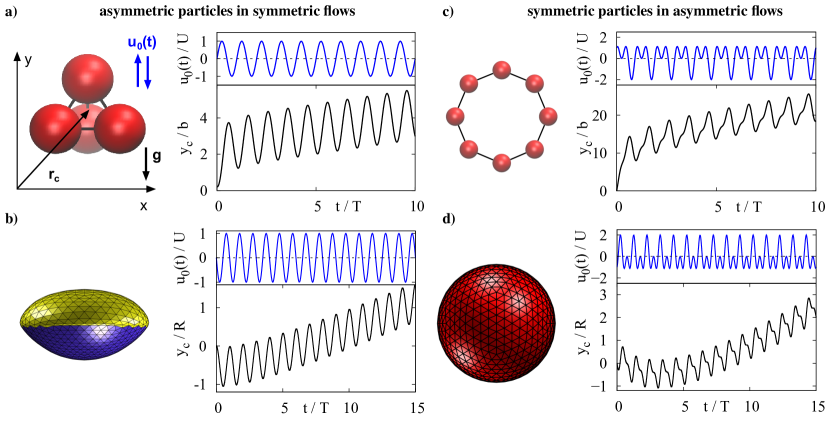
Figure 1: Sketch of four different particles with a mass density different from that of the surrounding liquid. The liquid shaken with the velocity ${\bf u}_{0}(t)=u_{0}(t){\bf e}_{y}$ causes an inertia-driven particle locomotion. The actuation is indicated by the motion of the particle’s center of mass ${\bf r}_{c}(t)=y_{c}(t){\bf e}_{y}$. Part a) shows an asymmetric bead-spring tetrahedron and part b) an asymmetric Janus capsule with different stiffness of each half (soft part yellow). Both asymmetric particles are considered in a sinusoidal velocity of the liquid with period $T$, as indicated by the upper blue curves in a) and b). We observe for both particles a net motion along the direction of shaking against gravitation, as described by the black curves in a) and b). The ring in c) and the symmetric capsule in d) are shaken by non-symmetric velocities as indicated by the blue curves in part c) and d). Also the ring and the symmetric capsule show a net progress against gravity as indicated by the black curves in c) and d). Parameters are given in sections 2 and 4.

In this work we show that the inertia induced passive swimming of realistic and experimentally available soft particles in oscillatory liquid motion can outweigh gravitation. We show this at first for an Janus capsule with an asymmetric elasticity (see e.g. [25]). We explain that an intrinsic particle asymmetry is not required for passive swimming and we demonstrate that the inertia driven particle propulsion works also for the much wider class of homogeneous and symmetric soft particles, such as soft capsules. This is achieved by appropriately engineering the time-dependence of shaking the liquid. The time-dependence of the shaking determines also the direction of passive swimming. This motion is distinct from particle locomotion in oscillatory flows at finite Re, where propulsion is related to streaming flows and a fluid jet in the wake of the swimmer [26].

The work is organized as follows: In section 2 we describe the modeling and simulation of the particles sketched in figure 1. We show in section 3 by an approximate analytical approach, that the locomotion of non-buoyant soft particles in a periodically oscillating fluid motion requires the symmetry breaking caused by different particle deformations and Stokes drags during the two half-periods of the shaking of the liquid. The analytical results are confirmed in section 4 by numerical simulations of the bead-spring models and capsules shown in figure 1. We study an asymmetric bead-spring tetrahedron in a sinusoidal liquid motion and a symmetric semiflexible bead-spring ring in a non-symmetric periodic liquid motion for a wide parameter range. The results of these simulations are complemented and verified by Lattice Boltzmann simulations of realistic soft asymmetric Janus capsules and symmetric capsules. For instance, we provide parameter ranges where the passive locomotion mechanism outweighs gravitation. Discussions of the results and the conclusions are given in sec. 5.

2 Model and Approach

The dynamics of four deformable particles in a shaken liquid is investigated by taking into account particle inertia. We use two asymmetric particles, namely a bead-spring tetrahedron composed of four beads, and a Janus capsule, as sketched in figures 1 a) and b), respectively. As examples of common symmetric particles we choose a bead-spring ring, as shown in figure 1c), and a symmetric capsule, as shown in figure 1d). The positions and the motion of the beads of the ring are restricted to the $(x,y)$ plane.

The shaking velocity of the liquid is given by

$$\mathbf{u}_{0}(t) =u_{0}(t)\hat{e}_{y}=U\,\left[\sin\left(\omega t\right)+\varepsilon\cos\left(2\omega t\right)\right]\hat{e}_{y}\,,$$ (1)

with the frequency $\omega=2\pi/T$ and a vanishing mean velocity $\langle\mathbf{u}_{0}(t)\rangle=0$. For $\varepsilon=0$ the velocity is sinusoidal and antisymmetric with respect to a shift $t\to t+T/2$, i.e., ${\bf u}_{0}(t)=-{\bf u}_{0}(t+T/2)$. For $\varepsilon\not=0$ this symmetry is broken and the velocity of the liquid is non-symmetric as indicated by the blue curves in figures 1c) and 1d).

In section 2.1 we describe the modeling of the bead-spring models and the capsules. In section 2.2, we present the equations of motion of the bead spring models, the Maxey and Riley equations [27] for several beads. They take the particle inertia into account and are extended by the hydrodynamic particle-particle interaction via the dynamical Oseen-tensor. The Lattice-Boltzmann-Method (LBM) for the particle simulations is explained in section 2.3.

2.1 Modeling the bead-spring models and the capsules

The beads of the bead-spring models have the mass $m_{i}$. Their mass density $\rho_{i}$ may be different from the mass density of the fluid, $\rho_{f}\not=\rho_{i}$. With the gravitational force along the negative $y$ direction, this leads to the buoyancy force

$${\bf F}_{g,i}=-F_{g,i}{\bf e}_{y},$$ (2)

which acts on a particle immersed in the liquid with

$$F_{g,i}=gV_{i}(\rho_{i}-\rho_{f})=g(m_{i}-m_{f})\,.$$ (3)

The tetrahedron in figure 1a) consists of $N=4$ beads at positions $\mathbf{r}_{i}$. The beads have the same radius $a$, but may have different masses. They are connected by springs with the stiffness $k$. The center of mass is given by

$$\mathbf{r}_{c}=\frac{1}{\sum_{i}m_{i}}\sum_{i}m_{i}\mathbf{r}_{i}\,.$$ (4)

Each bead experiences a force that is composed of the buoyancy force ${\bf F}_{g}$ and forces imposed by springs,

$$\mathbf{F}_{i}^{(P)}=-F_{g,i}\hat{e}_{y}-\nabla_{i}V_{spring}$$ (5)

with the spring potential

$$V_{spring}=\sum\limits_{i,j\neq i}^{N}k(|\mathbf{r}_{i}-\mathbf{r}_{j}|-b)^{2}\,\\$$ (6)

and the undistorted spring length $b$.

Also for the bead-spring model shown in figure 1c) (with $N=8$ beads) the neighboring beads are connected by Hookean springs. In addition to equation (5) a bending potential with the stiffness $\kappa$ is taken into account

$$V_{bend}=-\frac{\kappa}{2}\sum\limits_{i=1}^{N}\ln\left(1+\cos\beta_{i}\right)\,$$ (7)

where ${\bf R}_{i}={\bf r}_{i}-{\bf r}_{i+1}$ is the the bond vector between the next-neighbor beads $i$ and $i+1$ and the angle $\beta_{i}$ is defined via $\cos\beta_{i}={\bf{e}}_{R_{i-1}}\cdot{\bf{e}}_{R_{i}}$ with the bond unit vectors ${\bf{e}}_{R_{j}}={\bf R}_{j}/R_{j}$. This bending potential causes a circular ring shape in equilibrium.

The capsules are modeled by discretizing their surface with $N=642$, which is done iteratively as described in more detail in Ref. [28]. We assume that the surface is thin and has a constant surface shear elastic modulus $G_{s}$. In this case the relation between the deformation and the forces is given by the neo-Hookean law described by the potential $V_{NH}$ (for details we refer to  [29, 30]). Furthermore a bending potential $V_{b}$ is assumed [31, 32], which is given by

$$V_{b}=\frac{\kappa_{c}}{2}\sum\limits_{i,j}\beta_{i,j}^{2}\,,$$ (8)

where $\kappa_{c}$ denotes the bending stiffness and $\beta_{i,j}$ is the angle between the normal vectors of neighboring triangles.

For Janus capsules the stiffness is different in both halves of the capsule, as indicated in figure. 1(c). We use a penalty force to keep the capsule’s volume ${\cal V}(t)$ close to the reference volume ${\cal V}_{0}$ during the simulations. Its potential $V_{v}$ is given by

$$V_{v}=\frac{k_{v}}{{\cal V}_{0}}({\cal V}(t)-{\cal V}_{0})^{2}\,$$ (9)

with the rigidity $k_{v}$ [32]. The complete potential related to the forces acting on the capsule is given by

$$V({\bf r})=V_{NH}+V_{b}+V_{v}.$$ (10)

2.2 Maxey and Riley equations, including the dynamic Oseen-Tensor

The dynamics of the beads is described by the equations for the particle velocities ${\bf v}_{i}$ of Maxey and Riley [27]. The flow in presence of the particles is denoted by ${\bf u}({\bf r})$ and the flow field without the particles as ${\bf u}_{0}({\bf r})$ (given by equation (1)). The flow in presence of the particles must fulfill the conditions

$$\rho_{f}\frac{\partial\bf u}{\partial t} = \rho{\bf g}-\nabla p+\eta\Delta{\bf u},$$ (11)

$$\nabla\cdot{\bf u} = 0$$ (12)

$${\bf u}({\bf r}) = {\bf u}_{0}({\bf r})\mbox{ at }|{\bf r}|\rightarrow\infty$$ (13)

and no slip boundary conditions on the surface of the beads. The equation of motion of the spheres is

$$m_{i}\frac{d{\bf v}_{i}}{dt}=m_{p}{\bf g}+\oint\sigma d{\bf A}_{i}\,,$$ (14)

i.e. the integral over the stress tensor must be calculated. In this equation 14, the inertia of the beads is considered by the term $m_{i}\frac{d{\bf v}_{i}}{dt}$. This inertia of the particle is often neglected in bead spring models, but becomes important e.g. if the external flow has a high enough frequency (see sec. 14). This inertia can also occur if the Reynolds number of the flow around the particle is zero. The Reynolds number influences only the flow and thus the integral over the stress tensor in eq. (14). To calculate the integral in equation 14, a small Reynolds number, defined by $\mbox{Re}=\rho_{f}aw/\eta$ with the relative velocity ${\bf w}$ between the fluid velocity ${\bf u}_{0}$ and the particles velocity ${\bf v}$ is assumed, which allows to neglect the advective terms in the Navier-Stokes equation. We keep the time-derivative ${\partial_{t}\bf u}$ due to the high Strouhal number. The calculation of the integral over the stress tensor is given in [27] and leads to the following forces on the beads:

A bead experiences besides ${\bf F}_{i}^{(P)}$ the inertial force

$$\mathbf{F}_{i}^{(0)}=m_{f,i}\frac{d\mathbf{u}_{i}}{dt}\,$$ (15)

caused by the liquid acceleration at the position ${\bf r}_{i}$ of the bead. Note that the liquid velocity includes the externally imposed homogeneous liquid motion ${\bf u}_{0}(t)$ described in equation (1) and the flow perturbations caused by the motion of all other particles with respect to the liquid. Furthermore, the force ${\bf F}_{i}^{(1)}$ created by the difference between the particle velocity ${\bf v}_{i}$ and the liquid velocity ${\bf u}_{i}$ must be considered. This is composed of three contributions, the added mass, the Stokes drag and the Basset force,

$$\mathbf{F}_{i}^{(1)} = -\frac{1}{2}m_{f,i}\frac{d}{dt}\left(\mathbf{v}_{i}-\mathbf{u}_{i}\right)-\zeta_{b}(\mathbf{v}_{i}-\mathbf{u}_{i})$$ (16)

$$\qquad-6\pi\eta a^{2}\int_{0}^{t}d\tau\frac{\frac{d}{d\tau}\left[\mathbf{v}_{i}(\tau)-\mathbf{u}_{i}(\tau)\right]}{\sqrt{\pi\nu(t-\tau)}}\,,$$

with the Stokes drag coefficient $\zeta_{b}=6\pi\eta a$. Alltogether we obtain the dynamical equation for the velocity of the $i$th bead

$$m_{i}\frac{d\mathbf{v}_{i}}{dt}=\mathbf{F}_{i}^{(0)} + \mathbf{F}_{i}^{(1)}+\mathbf{F}_{i}^{(P)}\,.$$ (17)

The flow disturbances at ${\bf r}_{i}$ caused by all the other beads are determined via the dynamic Oseen tensor [33], which is the Greens function of the time-dependent linear Stokes equation. This provides the flow at the $i$th bead

$$\mathbf{u}_{i}=\mathbf{u}_{0}(t)+\sum\limits_{j\neq i}\int\limits_{0}^{t}dt^{\prime}\ \mathbf{H}_{i,j}(t^{\prime})\cdot\mathbf{F}_{j}^{(1)}(t^{\prime})\,.\\$$ (18)

For the explicit expression of $\mathbf{H}_{i,j}(t^{\prime})$ we refer to A.

Equation (16) is solved numerically for the bead-spring tetrahedron as shown in figure 1a) and for the bead-spring ring shown in figure 1c) by using a Runge-Kutta-scheme of fourth order. The dimensionless parameters given below are used for simulations of equation (17) for the bead-spring tetrahedron and the bead-spring ring. These parameters can be converted to SI units if the dimensionless time is multiplied by the factor $s_{t}=1\ \mbox{ms}$, the length by $s_{l}=50\ \mu\mbox{m}$ and mass by $s_{m}=5.2\cdot 10^{-13}\ \mbox{kg}$. This leads to the density and viscosity of water ($\rho_{water}=1000\ \mbox{kg}/\mbox{m}^{3}$, $\eta_{water}=1\mbox{ mPas }$) and the correct gravitational acceleration $g\approx 10\ \mbox{m}/\mbox{s}^{2}$.

The Parameters used in simulations of the bead-spring tetrahedron are: number of beads $N=4$, bead radius $a=0.1$, equilibrium spring length $b=0.25$, spring stiffness $k=15000$, mass density $\rho_{i}=3600$ of a bead, mass density of the fluid $\rho_{f}=240$, fluid viscosity $\eta=100.0$, amplitude of the shaking velocity $U=10.0$ in equation (1), asymmetry parameter $\varepsilon=0$, shaking period $T=0.4$, gravitational acceleration $g=0.21$ and time step $dt=2.5\cdot 10^{-4}$ in numerical integrations of equation (17).

The Parameters used in simulations of the semiflexible bead-spring ring are: number of beads $N=8$, bead radius $a=0.1$, equilibrium spring length $b=0.5$, spring stiffness $k=2000$, bending stiffness $\kappa=500$, mass density $\rho_{i}=3600$ of a bead, mass density of the liquid $\rho_{f}=240$, viscosity of the liquid $\eta=100$, amplitude $U=20$ of the shaking velocity in equation (1), asymmetry parameter $\varepsilon=0.8$, shaking period $T=0.4$, gravitational acceleration $g=0.21$ and time step $dt=2.5\cdot 10^{-4}$ in numerical integrations of equation (17).

Especially the flow amplitude is varied which leads to Reynolds numbers $\mbox{Re}=\rho_{f}Ub/\eta$ ranging from $0$ to $6$ and Strouhal numbers $\mbox{St}=b/(TU)$ ranging from $0.06$ to $\infty$. Due to the high range of the Strouhal number the time-derivative in the Navier-Stokes equation is kept. We neglect the advective terms in the Navier-Stokes equation to show that the locomotion of the particles is not induced by the non-linearity of the Navier-Stokes equation but by the simple Stokes drag. To verify this approximation the qualitative results are compared with simulations of the lattice-Boltzmann Method, which solves the full Navier-Stokes equation.

2.3 The Lattice Boltzmann Method

We use also the LBM to simulate the full Navier–Stokes equation including the dynamics of the particles. We utilize the common D3Q19 lattice-Boltzmann method (LBM) to simulate the distribution $f(\mathbf{x},t)$ of the fluid elements on a 3D grid of positions $\mathbf{x}_{i}=(x,y,z)$ along the discrete directions $\mathbf{c}_{i}$ ($i=0,\dots,19$) [34]. The lattice constants are $\Delta x=1$ for spatial and $\Delta t=1$ for temporal discretization. The evolution of the distribution function is governed by the discrete Boltzmann equation

$$f_{i}(\mathbf{x}+\mathbf{c}_{i}\Delta t,t+\Delta t)=f_{i}(\mathbf{x},t)+\mathcal{C},$$ (19)

where $\mathcal{C}$ defines the collision operator. Walls are incorporated by the standard bounce back scheme (bb) [35, 36] by adding the contribution $\mathcal{W}=2w_{i}\rho\frac{\mathbf{c}_{i}\cdot\mathbf{u}_{w}}{c_{s}^{2}}$ for wall links to equation (19) [37, 36], where $\mathbf{u}_{w}$ is the wall velocity. The weighting factor $w_{i}$ and the speed-of sound $c_{s}$ are constants for the chosen set of velocity directions [34].

Tetrahedron dynamics:

For the simulations of the tetrahedron, the Bhatnagar-Gross-Krook (BGK) collision operator

$$\mathcal{C}=-\frac{1}{\tau} \left[f_{i}(\mathbf{x},t)-f^{eq}_{i}(\mathbf{x},t)\right]+\mathcal{F}$$ (20)

is extend by the Guo force-coupling $\mathcal{F}=\Delta t\left(1-\frac{1}{2\tau}\right)w_{i}\left[\frac{c_{i}-\mathbf{u}}{c_{s}^{2}}+\frac{(\mathbf{c_{i}}\cdot\mathbf{u})}{c_{s}^{4}}\mathbf{c}_{i}\right]\cdot\mathbf{F}^{(e)}$ for external volume forces $\mathbf{F}^{(e)}$ [38]. $f^{eq}$ is an expansion of the Maxwell-Boltzmann distribution and $\tau$ is the relaxation parameter. The macroscopic density and momentum are obtained from the first two moments via $\rho=\sum_{i}f_{i}$ and $\rho\mathbf{u}=\sum_{i}\mathbf{c}_{i}f_{i}+\frac{\Delta t}{2}\mathbf{F}^{(e)}$, respectively. The viscosity of the fluid is given by $\nu=c_{s}^{2}\Delta t\left(\tau-1/2\right)$. The hard spheres are implemented as moving walls according to [35], with an additional lubrication-correction for squeezing motion of near particles, as discussed in [39]. This simulations are used to compare the Oseen simulations and the LBM simulations (see also B).

Capsule dynamics:

For the simulations of capsules, an adapted LBM-scheme of the multi-relaxation time LBM for a spatially dependent density is used [40]. The time evolution of the mean density $\rho_{0}(\mathbf{x},t)=\sum_{i}f_{i}+\frac{1}{2}\mathbf{u}\nabla\rho\Delta t$, the local density $\rho(\mathbf{x},t)$ and its gradient $\nabla\rho$ is used as input for the collision operator

$$\mathcal{C}= -S_{il}\left[f_{l}(\mathbf{x},t)-f_{l}^{eq}(\mathbf{x},t)\right]$$ (21)

$$+F_{i}(\mathbf{x},t)-\frac{1}{2}S_{il}F_{l}(\mathbf{x},t).$$

For the collision matrix $\mathbf{S}$ and its corresponding transformation matrix we use the set given in [41]. The correction term $F_{i}(\mathbf{x},t)=\Delta t\frac{(\mathbf{c}_{i}-\mathbf{u})}{c_{s}^{2}}\cdot\left[\nabla\rho c_{s}^{2}(\Gamma_{i}-w_{i})+\mathbf{F}^{(e)}\Gamma_{i}\right]$ accounts for the density inhomogeneity and external forces, with $\Gamma_{i}=w_{i}\left[1+\frac{\mathbf{e}_{i}\cdot\mathbf{u}}{c_{s}^{2}}+\frac{(\mathbf{c}_{i}\cdot\mathbf{u})^{2}}{2c_{s}^{4}}-\frac{|\mathbf{u}|^{2}}{2c_{s}^{2}}\right]$ [40]. The fluid velocity is linked to the density $\rho$ via the second moment $\rho\mathbf{u}=\sum_{i}f_{i}\mathbf{c}_{i}+\frac{1}{2}\mathbf{F}^{(e)}\Delta t$. The equilibrium distribution has the form $f_{l}^{eq}(\mathbf{x},t)=w_{l}\left[\rho_{0}+\rho\left(\frac{(\mathbf{c}_{l}\cdot u)}{c_{s}^{2}}+\frac{(\mathbf{c}_{l}\cdot\mathbf{u})^{2}}{2c_{s}^{4}}-\frac{|\mathbf{u}|^{2}}{2c_{s}^{2}}\right)\right]$. The capsule mesh is coupled to the LBM-grid via the immersed-boundary method using the four-point stencil [42]. The calculation of the field for the density $\rho(\mathbf{x},t)$ used in [40] is replaced by tracking nodes inside the capsule and setting $\rho(\mathbf{x},t)$ as $\rho_{capsule}$ inside and $\rho_{fluid}$ outside of the membrane and updating the capsule surface via the membrane-forces.

Oscillating flow.

To drive the oscillating flow, an external (volume-)force $\mathbf{F}^{(e)}_{flow}=U\rho\,\omega[\cos(t\omega)-2\varepsilon\sin(2t\omega)]\hat{\mathbf{e}}_{y}$ is applied to the LBM. To screen hydrodynamic self-interaction, we use bb walls in $x$ and $z$-direction with velocity $\mathbf{u}_{w}(t)=\mathbf{u}(t)$ to ensure Dirichlet boundary conditions of the flow.

Parameters and unit-conversion.

The used LBM parameters can be obtained from the SI parameters via the conversion values for length $s_{{L}}=7.57\cdot 10^{-7}\mbox{m}$, mass $s_{{M}}=4.348\cdot 10^{-16}\mbox{kg}$ and time $s_{{T}}=4.54\cdot 10^{-8}\mbox{s}$. All LBM simulations are performed with a viscosity $\eta=\eta_{water}=1\mbox{ mPas }$, gravitational acceleration $g=9.81\mbox{m}/\mbox{s}^{2}$, fluid density $\rho=\rho_{water}=1000\frac{\mbox{kg}}{\mbox{m}^{3}}$ and $k_{v}=2.78\cdot 10^{5}\frac{\mbox{kg}}{\mbox{s}^{2}\mbox{m}}$. The amplitude of the liquid’s velocity is $U=0.5\frac{\mbox{m}}{\mbox{s}}$ and the period is $T=90\mu\mbox{s}$ if not given otherwise. The cubic simulation box has a length of $1.14\times 10^{-4}$m.

3 Inertia driven actuation: Approximate analytical results

Soft particles are periodically deformed in shaken liquids, which causes a time-dependent viscous drag coefficient of the particle. How this deformability drives passive swimming of a particle in a shaken liquid is determined by an approximate analytical approach.

We discuss here a particle with a drag coefficient $\zeta_{tot}$. This already simplifies the dynamical equation (17). We further neglect the Basset force and the added mass in equation (16) but take the force $\mathbf{F}^{(0)}$ and the dominant viscous drag contribution to $\mathbf{F}^{(1)}$ into account. In this case we obtain the approximate dynamical equation for the velocity of a stiff particle

$$M\frac{d\mathbf{v}(t)}{dt}=\zeta_{tot}\left[\mathbf{u}_{0}(t)-\mathbf{v}(t)\right]+M_{f}\frac{d\mathbf{u}_{0}(t)}{dt}\,,$$ (22)

with the particle mass $M$, the displaced fluid mass $M_{f}$ and the constant Stokes drag coefficient $\zeta_{tot}$. To justify the validity of this approximations we compare them with the full numerical results in the next section.

For a sinusoidal liquid motion ${\bf u}_{0}(t)$ as described by equation (1) with $\varepsilon=0$ the solution of equation (22) is $\mathbf{v}(t)=v(t)\hat{e}_{y}$ with

$$v (t)=Ce^{-\frac{\zeta_{tot}}{M}t}+A\sin\left(\omega t+\phi\right)\,,$$ (23)

whereby

$$A = U\sqrt{\frac{M_{f}^{2}\omega^{2}+\zeta^{2}_{tot}}{M^{2}\omega^{2}+\zeta^{2}_{tot}}}=U\sqrt{\frac{\left({M_{f}\omega}/{\zeta_{tot}}\right)^{2}+1}{\left({M\omega}/{\zeta_{tot}}\right)^{2}+1}}$$ (24)

is the amplitude of the particle oscillation and the phase shift relative to the time-dependent liquid motion is given by

$$\phi = -\arctan\left(\frac{\zeta_{tot}\omega(M-M_{f})}{MM_{f}\omega^{2}+\zeta^{2}_{tot}}\right).$$ (25)

The exponential contribution to equation (23) includes the relaxation time $\tau_{v}=\frac{M}{\zeta_{tot}}$ that the particle needs to adjust its velocity ${\bf v}$ to the velocity of the liquid ${\bf u}_{0}$. We approximate this time scale by

$$\tau_{v}=\frac{M}{\zeta_{tot}}\approx\frac{4m}{4\zeta_{b}}=\frac{m}{\zeta_{b}}\,$$ (26)

for the bead spring models and for the capsule by

$$\tau_{v}=\frac{M}{\zeta_{tot}}=\frac{2R^{2}\rho}{9\eta}$$ (27)

with

$$\zeta_{tot}=6\pi\eta R\,,\quad V=\frac{4}{3}\pi R^{3}\,,\quad M=\rho V.$$ (28)

We discuss in the following the case $M\geq M_{f}$ (but also $M<M_{f}$ is possible). For a high friction or slow frequency, i.e. $\frac{M}{\zeta_{tot}}\omega\ll 1$, the particle velocity adjusts rather quickly to the liquid motion. This means the particle quickly adapts to the motion of the liquid, i.e. $A\rightarrow U$ and $\phi\rightarrow 0$ (cf. equations (24) and (25)) and the particle’s inertia is negligible in this case.

In the range $\frac{M}{\zeta_{tot}}\omega\gtrapprox 1$ the particle’s inertia becomes important and it can not follow the liquid velocity, which results in $A<U$, $\phi<0$. This lag behind of the particle can be used to achieve a non-vanishing mean velocity: If the shape of the deformable particle and therefore the drag is different in each half cycle of the shaking, as indicated in figure 2b), the delay of the particle with respect to the fluid is different in each half cycle. This difference may finally lead to a net motion of the particle with respect to the fluid. Since the liquid does not move in the mean, this relative net motion results in an absolute particle actuation.

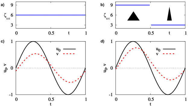
Figure 2: We consider a particle of mass $M$ different from the surrounding liquid of mass $M_{f}$ for the identical volume. We assume a sinusoidal fluid velocity $u_{0}(t)$ given by equation (1) for $\varepsilon=0$, see also solid lines in c) and d). If the shape and the Stokes drag of the particle is constant in time, the particle velocity is also a sinusoidal, but has a smaller amplitude and follows with a small phase shift (dashed line in figure c)). For a different shape and a Stokes drag in both half periods, i.e. $\zeta_{1}\not=\zeta_{2}$, the particle velocity is also differently, as indicated by the dashed line in figure d). This leads to a different mean velocity of the particle in each half cycle. Therefore, the actuation step is different in each half cycle which results in a net particle actuation. Parameters: $U=1$, $T=1$, $M_{f}=1$, $M=2$.

In order to gain further analytical insight, we consider an asymmetric, i.e. anisotropic, deformable particle as illustrated in figure 2b). We assume a fixed shape and therefore a fixed Stokes drag during each half period as described by

$$\zeta_{tot}(t)=\left\{\begin{array}[]{l}\zeta_{1}\mbox{ at }0<t<\frac{T}{2}\,,\\ \zeta_{2}\mbox{ at }\frac{T}{2}<t<T\,,\end{array}\right.$$ (29)

and continued analogously in the following periods. These two different constant values of the Stokes drag just mimic the essence of the different time-dependent shapes and Stokes drags of the particles sketched in figure 1. Numerical results of the full equations, i.e. that include the deformations of the particles, are given in the next section.

For a sinusoidal liquid velocity the particle velocities in both half periods are

$$v_{1,2}(t)=C_{1,2}e^{-\frac{\zeta_{1,2}}{M}t}+A_{1,2}\sin\left(\omega t+\phi_{1,2}\right)\,,$$ (30)

whereby $A_{i}$ and $\phi_{i}$ are calculated as given in equations (24) and (25) but with the according value of $\zeta_{tot}(t)$. Due to the periodic liquid motion, the boundary conditions for the particle velocities are

$$v_{1}(0)=v_{2}(T),\qquad v_{1}\left(\frac{T}{2}\right)=v_{2}\left(\frac{T}{2}\right)\,.$$ (31)

This allow the determination of the constants $C_{1,2}$ as

$$C_{1} = -U\omega\Gamma\frac{(\omega^{2}M^{2}-\zeta_{1}\zeta_{2})(e^{-\frac{2\zeta_{2}\pi}{\omega M}}+e^{-\frac{\zeta_{2}\pi}{\omega M}})}{e^{-\frac{\pi(\zeta_{1}+2\zeta_{2})}{\omega M}}-e^{-\frac{\zeta_{2}\pi}{\omega M}}}\,,$$ (32)

$$C_{2} = -U\omega\Gamma\frac{(\omega^{2}M^{2}-\zeta_{1}\zeta_{2})(1+e^{-\frac{\zeta_{1}\pi}{\omega M}})}{e^{-\frac{\pi(\zeta_{1}+2\zeta_{2})}{\omega M}}-e^{-\frac{\zeta_{2}\pi}{\omega M}}}$$ (33)

with the abbreviation

$$\Gamma=\frac{(\zeta_{1}-\zeta_{2})(M-M_{f})}{(\omega^{2}M^{2}+\zeta_{2}^{2})(\omega^{2}M^{2}+\zeta_{1}^{2})}\,.$$ (34)

The mean velocity of the particle is then given by

$$v_{n} = \frac{\int_{0}^{T}v(t)dt}{T}$$ (35)

$$= \Gamma\ \frac{U\omega^{2}M}{2\zeta_{1}\zeta_{2}\pi}\left[(\zeta_{1}+\zeta_{2})(\zeta_{1}\zeta_{2}+\omega^{2}M^{2})\right.$$

$$\qquad+\left.(\zeta_{1}-\zeta_{2})(\omega^{2}M^{2}-\zeta_{1}\zeta_{2})\frac{\exp\frac{\zeta_{2}\pi}{\omega M}-\exp\frac{\zeta_{1}\pi}{\omega M}}{\exp\frac{\pi(\zeta_{1}+\zeta_{2})}{\omega M}-1}\right]\,.$$

The equations (34) and (35) allows to discuss the requirements of a particle actuation, i.e. a non-vanishing mean velocity $v_{n}$ and its direction. All factors of the product in equation (35) are positive (with assuming $U>0$), except $\Gamma$, so that the direction of the motion is determined by $\Gamma$ (this is shown in C). Furthermore, to achieve a mean velocity the factor $\Gamma$ must not be zero. This means firstly that the mass density of the particle and the surrounding fluid must differ, i.e. $M\not=M_{f}$. In addition the drag coefficients in both half cycles have to be different, i.e., $\zeta_{1}\not=\zeta_{2}$. This is further illustrated in figure 2.

For an equal mass density of the particle and the liquid, $M=M_{f}$, the particle follows the fluid motion instantaneously and the mean velocity vanishes. For $M\not=M_{f}$ but identical drag coefficients in both half periods, as in figure 2a), the fluid velocity ${\bf u}_{0}$ and the particle velocity ${\bf v}(t)$ are both sinusoidal as indicated in figure 2c). Both velocities have a different amplitude and there is a relative phase shift, but there is again no net progress of the particle.

If the shape and drag coefficients of the anisotropic particle in figure 2b) are different in both half cycles of the shaking, i.e. $\zeta_{1}\not=\zeta_{2}$, then one has a non-symmetric velocity ${\bf v}(t)$ of the particle as shown in figure 2d). This asymmetry of ${\bf v}(t)$ causes a net progress of the particle per cycle.

The net progress of a deformable particle depends strongly on the relaxation time $\tau_{v}$. For a small frequency, i.e., $\tau_{v}\omega\ll 1$, one obtains only a small actuation because the particle follows the liquid’s motion nearly instantaneously, i.e. ${\bf v}(t)\approx{\bf u}_{0}$. This means $v_{n}\rightarrow 0$ for $\omega\rightarrow 0$ which follows also with equation (35).

The direction is determined by $\Gamma$ (eq. (34)) if $U>0$ is assumed. This means the direction is given by the half period with the higher drag coefficient, i.e. by $\zeta_{1}$ or $\zeta_{2}$. It is also important if the particle has a higher or lower density than the surrounding fluid which determines if $M_{f}<M$ or $M_{f}>M$. With $M_{f}<M$ the particle lags behind the flow and with a lighter particle $M_{f}<M$ the opposite is the case.

Hence the requirements of the particle actuation can be discussed with equation (35). Note that it takes the particle inertia into account, i.e. the terms proportional to the mass of the particle in eqs. (14), (17) or (22) are important. The fluid Reynolds number is not important for the actuation, because the Stokes friction in equation (22) occurs also at a low Reynolds number.

A time-dependence of the drag coefficient can be achieved with a soft particle in a shaken fluid. The difference in the drag coefficient in both half periods, i.e. $\zeta(t)\neq\zeta(t+T/2)$, (as sketched in figure 2b)) can be achieved with an asymmetric particle in a sinusoidal shaken fluid. In case of a symmetric soft particle a different shape and therefore a different drag coefficient of the particle in each half cycle can be achieved by a non-symmetric periodic fluid velocity ${\bf u}_{0}(t)$ with $\varepsilon\not=0$ in equation (1). This is further exemplified in the next section.

To compare the approximation in this section for ${\bf v}$ and the results from simulations in the next section, gravity must be taken into account. Gravity leads approximately to the additional contribution

$$v_{s}=\frac{g}{2}\left(\frac{M_{f}-M}{\zeta_{1}}+\frac{M_{f}-M}{\zeta_{2}}\right)\,$$ (36)

to the mean actuation velocity, cf. equation (35).

4 Numerical Results

In this section, we explore numerically the inertia driven dynamics and locomotion of four soft particles in a shaken liquid, which are sketched in figure 1. The selected numerical simulations are guided by the results of the previous section i.e., particle locomotion is expected in parameter ranges with different mass densities of the particles and the liquid and the Stokes drag of a particle is is unequal during each half of a shaking period $T$. Such a time-dependent Stokes drag can be realized by asymmetric particles but also with symmetric ones.

Firstly, the dynamics of the asymmetric particles is investigated for the sinusoidal shaking velocity ${\bf u}_{0}$ in equation (1) with $\varepsilon=0$. We show simulations of the bead-spring tetrahedron in section 4.1 and compare the results with a more realistic Janus capsule in section 4.2. The intrinsic anisotropic of both particles causes different deformations and Stokes drags during each half period of the sinusoidal velocity ${\bf u}_{0}$.

Secondly, symmetric particles are investigated. To achieve different deformations and Stokes drags during the two halves of the shaking period for these particles as well, we utilize a non-symmetric shaking velocity in equation (1) with $\varepsilon\not=0$. We discuss the dynamics of a symmetric bead-spring ring and show that a symmetric capsule behaves similar to the ring in section 4.4.

All particles are soft particles with a different mass density than the liquid. They are deformed in shaken liquids, which is taken into account in the numerical simulations. Hence, besides the velocity relaxation time $\tau_{v}$ (cf. equations (26) and (27)) considered in sec. 3, also the shape relaxation time $\tau_{k}$ and especially the ratio $T/\tau_{k}$ are important. The shape relaxation time is given by the time the particles needs to relax to their equilibrium shape after a deformation. To determine the order of the relaxation-time scale, we use as an estimate for the bead spring models

$$\tau_{k}\approx\sqrt{\frac{m}{k}}$$ (37)

with the spring constant $k$, cf. equation (6), and the bead mass $m$ and for the capsules

$$\tau_{k}\approx\sqrt{\frac{\rho_{capsule}V}{G}}$$ (38)

with the capsule volume $V$ and the surface shear elastic modulus $G$.

4.1 Actuation of a tetrahedron in a sinusoidally shaken liquid

We investigate at first the motion of asymmetric particles in a sinusoidally shaken fluid. We begin with the simple bead-spring tetrahedron. Two orientations of the bead-spring tetrahedron in a vertically shaken fluid are investigated, one with a corner upward ($\blacktriangle$), cf. figure 3a), and one with a corner downward ($\blacktriangledown$). These positions are stable against a rotational perturbation. Figure 3a) shows the $\blacktriangle$-tetrahedron at four deformations during one period $T$ of a sinusoidally shaken liquid.

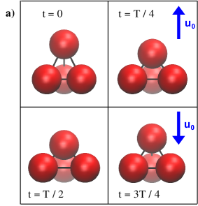
Figure 3: a) shows four snapshots of a deformable, upward oriented tetrahedron($\blacktriangle$) during one period $T$ in a sinusoidally shaken fluid. In b) the mean propulsion velocity $v_{n}$ of the tetrahedron is given for two ratios between the mass density of the beads and of the fluid, i.e. for $\rho/\rho_{f}=5,15$. $v_{n}$ is given in units of the related sedimentation velocities $v_{s,i}$, respectively. The $\blacktriangle$-tetrahedron outweighs gravity for $\rho/\rho_{f}=15$ in the range $U/v_{s,15}\gtrsim 160$ and rises in the shaken liquid. For $\rho/\rho_{f}=5$ the $\blacktriangle$-tetrahedron rises in the range $U/v_{s,15}\gtrsim 210$. The sedimentation velocity of the $\blacktriangledown$-tetrahedron is enhanced by liquid shaking as indicated by the dash-dotted line. Parameters: see section 2.2.

The center of mass of the tetrahedron, $y_{c}(t)$, follows via the viscous drag the oscillatory motion of the shaken liquid. Moreover, $y_{c}(t)$ exhibits besides an oscillatory motion also a mean net propulsion as indicated in figure 1a). The resulting mean velocity $v_{n}$ of the center of mass, which is studied in the following, is determined by fitting a straight line to $y_{c}(t)$ over a sufficient number of periods after a transient phase. The parameters for the numerical studies are given in section 2.2. We give the mean velocity $v_{n}$ and the amplitude $U$ of the shaking velocity in units of the sedimentation velocity (absolute value) denoted by $v_{s,r}$, whereby the index $r$ indicates the ratio of the density of the tetrahedron and the fluid, $\rho/\rho_{f}=r$. The sedimentation velocities $v_{s,5}=8.9\cdot 10^{-3}$ and $v_{s,15}=3.1\cdot 10^{-2}$ (absolute values) are determined without a shaking of the liquid (pure sedimentation).

In figure 3b) we show the mean velocity $v_{n}$ of the tetrahedra in the gravitational field as function of the amplitude $U$. For the $\blacktriangle$-tetrahedron for two ratios $\rho/\rho_{f}=5,15$ and for the $\blacktriangledown$-tetrahedron for $\rho/\rho_{f}=15$. The sedimentation velocity $v_{s,r}$ and $v_{n}$ increase with the density ratio $\rho/\rho_{f}$. For $\blacktriangle$-tetrahedra the mean velocity $v_{n}$ becomes positive for $\rho/\rho_{f}=15$ beyond $U/v_{s,15}\gtrsim 160$ and for $\rho/\rho_{f}=5$ beyond $U/v_{s,15}\gtrsim 210$. In both ranges the locomotion of a tetrahedron outweighs the downward oriented gravitation and heavy particles can be elevated. Therefore, for smaller mass differences between soft particles and the liquid this locomotion mechanism becomes less effective and a higher velocity amplitude $U$ is required to outweigh gravitation. A downward orientated shaken heavy tetrahedron ($\blacktriangledown$) will sediment faster than without shaking. Furthermore, a buoyant particle with $\rho/\rho_{f}=1$ follows the oscillatory liquid motion and its mean velocity $v_{n}$ vanishes in agreement with the reasoning given in the previous section. The inertial actuation is also found for tetrahedra lighter than the liquid, i.e. $\rho/\rho_{f}<1$. Note that the dependence on the initial condition can be avoided by an asymmetric mass distribution of the beads, because this leads to a reorientation of the tetrahedron. For example with one bead lighter than the other three beads, the lighter bead will point upwards after a certain time. The inertia driven actuation of such a tetrahedron is discussed in B.

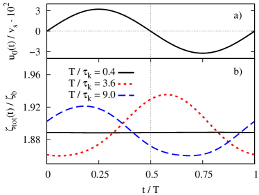
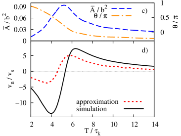
Figure 4: a) shows the shaking velocity $u_{0}(t)$ with $\varepsilon=0$ in equation (1) in units of the sedimentation velocity $v_{s}$ of an upward oriented tetrahedron ($\blacktriangle$) with $\rho/\rho_{f}=15$. The deformation of a tetrahedron, cf. figure 3a), is accompanied by a time-dependent Stokes drag $\zeta_{tot}$ as shown in b) (in units of $\zeta_{b}=6\pi\eta a$) for three different ratios $T/\tau_{k}$. c) shows the time-dependent deviation $\bar{A}$ from the mean area $A_{0}$ of the lower triangle of a $\blacktriangle$-tetrahedron, as defined in equation (39), as well as the phase shift $\Theta/\pi$ between the velocity $u_{0}(t)$ and the deformation. In d) the dependence of the mean velocity $v_{n}/v_{s}$ is given as a function of $T/\tau_{k}$ for the velocity amplitude $U/v_{s}\simeq 32$. The dashed line is obtained by equation (35) with $\zeta_{1,2}$. Parameters: $k=30000$ and those given in section 2.2.

The mean velocity $v_{n}$ depends also on ratio between the shaking period $T$ and the bead-spring relaxation time $\tau_{k}$ (cf. equation (37)). This dependence is shown in figure 4d) for a $\blacktriangle$-tetrahedron. This figure shows in part b) also the time-dependence of the drag coefficient of the tetrahedron, $\zeta_{tot}(t)$ (cf. A ), which is caused by the time-dependent deformation. Thus, in addition the deformation amplitude $\bar{A}$ of the bottom triangle of the tetrahedron with area

$$A(t)=\bar{A}\sin\left(\frac{2\pi}{T}t-\Theta\right)+A_{0}\,,$$ (39)

is given in figure 4c). Also the phase shift $\Theta$ of the deformation and the flow is shown. The area A(t) is determined by a fit to the data.

If $T$ is considerably smaller than the relaxation time $\tau_{k}$, the deformation of the tetrahedron cannot follow the liquid oscillation and remains small, as indicated for the deformation amplitude ${\bar{A}}$ in figure 4c). Consistently, the drag coefficient $\zeta_{tot}$ is nearly constant as indicated for $T/\tau_{k}=0.4$ in figure 4b). In this case particles just sediment in a shaken liquid. For larger $T$ the tetrahedron becomes deformed during liquid shaking and the drag coefficient $\zeta_{tot}(t)$ shows similar as $u_{0}(t)$ a sinusoidal time-dependence as indicated for $T/\tau_{k}=3.6$ in figure 4b). However, for such short shaking periods the tetrahedron deformation can still not follow the liquid oscillation and $\zeta_{tot}$ is nearly in antiphase to $u_{0}(t)$ as indicated by in figure 4b) and in figure 4c). Due to this phase shift for $T/\tau_{k}=3.6$ the Stokes drag in figure 4b) is larger during the downward liquid motion with $u_{0}(t)<0$ than during its upward motion. Therefore, the inertia induced locomotion is downward oriented for $T/\tau_{k}=3.6$ as also indicated in figure 4d) for the whole range $T/\tau_{k}\lesssim 5.7$. For $T/\tau_{k}=9$ beyond the maximum of $v_{n}/v_{s}$ in 4d) the deformation of the tetrahedron follows $u_{0}(t)$ more closely with a smaller phase difference $\Theta$ and the drag is slightly larger during the upward motion, cf. figure 4b). In this case and in the range $T/\tau_{k}\gtrsim 5.7$ the locomotion mechanism points into the opposite direction to the gravitation and can even outweigh gravitation for $U/v_{s}\simeq 32$, i.e., $v_{n}/v_{s}$ becomes positive. $v_{n}/v_{s}$ remains positive up to about $T/\tau_{k}\sim 27$ and beyond this ratio the tetrahedron sinks again due to the gravitation. This shows that indeed the time-dependent Stokes drag coefficient is a cause of the non-zero mean velocity. Note hereby that the model neglects the advective terms of the Navier-Stokes equation, i.e. they are not important for the actuation.

Besides the shape relaxation time also the velocity relaxation time $\tau_{v}$ (cf. equation (26)) plays a role as stated in section 3. We have chosen similar values of $\tau_{v}\approx 0.07$ and $\tau_{k}\approx 0.03$. The period $T$ is in the range $1\lesssim T/\tau_{v}\lesssim 6$, so that the particle’s inertia is significant.

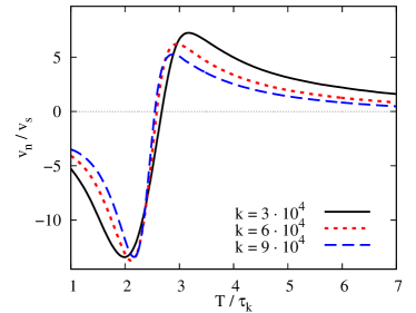
Figure 5: The mean locomotion velocity $v_{n}$ of the $\blacktriangle$-tetrahedron, cf. figure 3a), is given as a function of $T/\tau_{k}$ for three different values of the spring stiffness $k$ in equation (6) with $\rho/\rho_{f}=15$. The minima of the curve occur at similar values of $T/\tau_{k}\approx 2$ and the maxima at $T/\tau_{k}\approx 3$ despite different values of $k$.

One can also use the approximate mean velocity in equation (35) by selecting the drag coefficient $\zeta_{tot}$ from simulations of the tetrahedron. We use the maximal drag during each half period for $\zeta_{1,2}$. The resulting dependence of $v_{n}/v_{s}$ is indicated in figure 4d). This result confirms that the approximate approach presented in section 3 covers the essential inertia driven locomotion mechanism considered in this work.

In figure 5 the dependence of $v_{n}/v_{s}$ on the ratio $T/\tau_{k}$ is shown for different values of the spring constant $k$ of the tetrahedron. The extrema and the zero of $v_{n}/v_{s}$ are located at similar values of $T/\tau_{k}$. Moreover, the magnitudes of the minima and maxima of $v_{n}/v_{s}$ differ only slightly for different values of $k$. This emphasis again the importance of the ratio between shaking period and the particle’s relaxation time $\tau_{k}$

4.2 Actuation of a Janus capsule in a sinusoidally shaken liquid

With a Janus capsule that is composed of two parts of different elasticity we consider in this section a realistic soft anisotropic particle. The four snapshots shown in 6a) highlight the different deformations during a sinusoidal shaking cycle $T$. We investigate two orientations of the asymmetric Janus particle in the shaken liquid: One with the soft half on top as in figure 6a) (upward oriented Janus capsule $\blacktriangle$), or with the soft part at the bottom ($\blacktriangledown$). These orientations are stable against a rotational perturbation.

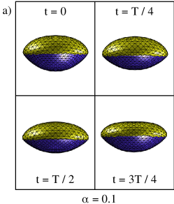
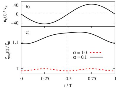
Figure 6: a) shows four snapshots of a deformable, with the soft side upward oriented Janus capsule ($\blacktriangle$) during a period $T$ in a shaken fluid with the elasticity ratio $\alpha=0.1$. Figure b) shows the sinusoidal shaking velocity $u_{0}(t)/v_{s}$ in units of the sedimentation velocity $v_{s}$ of the Janus capsule. The lower part in b) shows the Stokes drag $\zeta_{tot}(t)$ in units of the Stokes drag $\zeta_{0}=6\pi\eta R$ of the undeformed capsule for the elasticity ratio $\alpha=0.1$ (solid line) and the symmetric capsule with $\alpha=1$ (dashed line).

The capsule simulations are performed with the LBM and, besides the parameters given in section 2.3, the following values are used: radius of the capsule $R=10\mu\mbox{m}$, $\rho_{Janus}=2\rho_{fluid}$, $G^{(0)}=3.95\cdot 10^{-3}\mbox{kg}/\mbox{s}^{2}$ and $\kappa_{c}^{(0)}=3,77\cdot 10^{-13}\mbox{kg m}^{2}/\mbox{s}^{2}$. For the elastic properties of the second half of the capsule we set $\kappa_{c}^{(var)}=\alpha\kappa^{(0)}$ and $G^{(var)}=\alpha G^{(0)}$ with an elasticity ratio $\alpha=0.1$. This results in the two ratios $T/\tau_{k}\approx 2$ and $T/\tau_{v}\approx 2$ (cf. equations (27) and (38), determined with $G^{(0)}$), which ensure that the Janus capsule is deformed during the shaking of the liquid and that the inertia of the capsule is significant.

For Janus capsules neither the deformation nor the Stokes drag $\zeta_{tot}$ has a symmetry, i.e. $\zeta_{tot}(t)\neq\zeta_{tot}(t+T/2)$, as indicted for $\alpha=0.1$ by the snapshots in figure 6a) and in figure 6c), respectively. Therefore the time-dependence of $y_{c}(t)$ for a $\blacktriangle$ Janus capsule in figure 1b) displays the inertia induced locomotion (cf. figure 1b) ). This is not the case for the symmetric capsule with $\alpha=1.0$: The Stokes drag $\zeta_{tot}(t)$ given in figure 6c) has the symmetry $\zeta_{tot}(t)=\zeta_{tot}(t+T/2)$. Consequently, the symmetric capsule just sinks in a sinusoidally shaken fluid in the presence of gravitation.

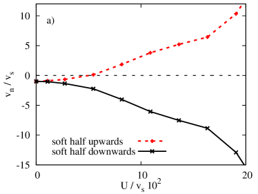
Figure 7: The mean actuation velocity $v_{n}$ of a Janus capsule is given as a function of the shaking-velocity amplitude $U$ in equation (1) with the soft side either upwards ($\blacktriangle$) or downwards ($\blacktriangledown$). In the $\blacktriangle$-case the capsule locomotion outweighs gravitation if $U\gtrsim 500\,v_{s}$ and $v_{n}$ becomes positive. In the $\blacktriangledown$-case the shaking of the liquid enhances the sinking velocity. b) shows $v_{n}/v_{s}$ for the $\blacktriangle$-capsule as function of the elasticity ratio $\alpha$. At $\alpha=1$ the particle sinks. By enhancing the asymmetry (decreasing $\alpha$) the capsule locomotion outweighs gravitation for $\alpha\lesssim 0.8$.

The mean velocity of the Janus capsule $v_{n}/v_{s}$ is shown in figure 7 as function of the velocity amplitude $U$. The sedimentation velocity of the $\blacktriangledown$ Janus capsule is enhanced by the oscillatory fluid motion as shown by the lower curve in 7a). For a velocity amplitude $U\gtrsim 500\,v_{s}$ (with $v_{s}\approx 0.15\frac{\mbox{mm}}{\mbox{s}}$) the locomotion of the $\blacktriangle$ capsule outweighs gravitation and moves upward, i.e., $v_{n}>0$. This is indicated by the dashed curve in 7a). As for the tetrahedron the locomotion increases with the difference between the mass density of the capsule and the liquid. This also means, the critical amplitude $U$ to outweigh gravitation is reduced by increasing the ratio $\rho_{capsule}/\rho_{liquid}$. The mean locomotion velocity $v_{n}/v_{s}$ for an upward oriented Janus capsule in a gravitational field is also shown as function of elasticity ratio $\alpha$ in figure 7b). This graph shows that the inertia induced locomotion increases with increasing elastic asymmetry (i.e., decreasing $\alpha$) and outweighs in the range $\alpha\lesssim 0.8$ gravitation for the given parameters. The symmetric capsule with $\alpha=1.0$ just sinks in the mean.

In figure 7a) the Reynolds number Re in LBM simulations is finite with $0\leq$ Re $\lesssim 3$ and an inertia induced capsule locomotion is found at small and intermediate values of the Reynolds number (and also beyond this values). The qualitative behavior of this capsule locomotion is similar as for the tetrahedron in the limit of vanishing Reynolds number. The reason is that the locomotion of the particles is driven by the inertia of the particles and the time-dependent stokes drag, which is both included in the model of the bead-spring tetrahedron.

4.3 Bead-spring ring in a non-symmetrically shaken liquid

In this and the following section, we explore the conditions for which also common symmetric soft micro-particles behave in shaken liquids as passive microswimmers. We begin with a symmetric bead-spring ring as sketched in figure 1. The parameters used in simulations are given in section 2.2 and the velocities are given in units of the sedimentation velocity $v_{s}=0.031$ (determined without shaking of the liquid).

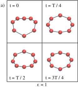
Figure 8: a) shows four snapshots of the bead-spring ring during one period $T$ of the liquid velocity as shown by the solid line in b) and as given by equation (1) for $\varepsilon=1$. In this case the drag coefficient $\zeta_{tot}(t)$ (in units of $\zeta_{b}=6\pi\eta a$) is different in both half periods as shown by the solid line in c), i.e., $\zeta_{tot}(t+T/2)\not=\zeta_{tot}(t)$. This causes a finite mean actuation velocity $v_{n}$. For $\varepsilon=0$ the shaking is sinusoidal, cf. dashed line in b), the drag coefficient is the same in both half periods of the shaking, i.e., $\zeta_{tot}(t)=\zeta_{tot}(t+T/2)$, and $v_{n}=0$.

Figure 8a) shows four snapshots of a bead-spring ring during one period $T$ of a non-symmetric shaking velocity $u_{0}(t)$ given by equation (1) and as shown in figure 8b) for $\varepsilon=1$. For a sinusoidally shaken liquid with $\varepsilon=0$ and $u_{0}(t)=-u_{0}(t+T/2)$ the drag coefficient $\zeta_{tot}(t)$ (cf. A ) is the same in both half periods with $\zeta_{tot}(t)=\zeta_{tot}(t+T/2)$, as indicated in figure 8c). In this case the ring exhibits no net actuation and sinks in the gravitational field. For a non-symmetric periodic shaking velocity with $\varepsilon\neq 0$ and $u_{0}(t)\neq-u_{0}(t+T/2)$ the drag coefficient of the ring is different in both half periods as shown for $\varepsilon=1$ in 8c). This leads to the passive swimming as shown in figure 1c).

Figure 9 shows the mean velocity $v_{n}$ of the bead-spring ring as a function of $\varepsilon$. For $\varepsilon\gtrsim 0.05$ the upward directed, inertia induced actuation is sufficiently strong to outweigh gravitation and $v_{n}$ becomes positive. For $\varepsilon<0$ liquid shaking enhances the sedimentation velocity. Thus the sign of $\varepsilon$ determines the direction of the inertia induced actuation of the semiflexible ring.

Figure 9: The mean actuation velocity $v_{n}$ varies linearly with the modulation parameter $\varepsilon$ of the shaking velocity in equation (1). For sufficiently positive values $\varepsilon\gtrsim 0.05$ the liquid shaking outweighs gravitation and $v_{n}$ becomes positive. For sinusoidal shaking with $\varepsilon=0$ the particle sinks due to gravity and at negative values of $\varepsilon$ the inertial actuation leads to an enhanced sedimentation velocity.

The mean velocity $v_{n}$ is given as function of the amplitude $U$ of the shaking velocity in figure 10. Without shaking at $U=0$ the ring sinks. With increasing values of $U$ and $\varepsilon=1$ the sinking velocity slows down until it turns over to an upward motion at larger values $U\gtrsim 225v_{s}$.

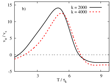
Figure 10: a) shows the mean propulsion velocity $v_{n}$ as a function of the shaking amplitude $U$. For positive $\varepsilon$ the actuation is upward directed and for $\varepsilon=1$ it outweighs gravitation in the range $U\gtrsim 225v_{s}$, i.e., $v_{n}$ becomes positive. b) shows the mean velocity of the ring as a function of the ratio ${T}/{\tau_{k}}$ for two different values of the spring stiffness $k$. At small values of ${T}/{\tau_{k}}$ the ring can not follow the liquid motion, it is not deformed and just sinking. At intermediate values ${T}/{\tau_{k}}$ the mean velocity becomes positive for both values of $k$ with a maximum in the range ${T}/{\tau_{k}}\approx 5$. For longer shaking periods the ring sinks again.

The mean velocity $v_{n}$ depends also on the ratio between the shaking period and the relaxation time $T/\tau_{k}$ as shown in figure 10b) for two values of the spring stiffness $k$. At small values of ${T}/{\tau_{k}}\lesssim 0.4$ the ring sinks because the shaking period is too small to cause sufficient deformations and differences between the Stokes drags during the two half periods. For longer periods $T$ and intermediate values of $T/\tau_{k}$ the acceleration induced shape and Stokes drag changes of the ring become sufficiently strong to outweigh gravitation. For both spring constants $k$ the mean velocity becomes positive in a wide range and reaches its maximum at a value of ${T}/{\tau_{k}}\approx 5$ due to the large deformation, as indicated in figure 10b). At higher values of ${T}/{\tau_{k}}$ the deformation becomes smaller and therefore the ring sinks again due to gravitation. The values of the shape relaxation time $\tau_{k}\approx 0.08$ (cf. equation (37)) and the velocity relaxation time $\tau_{v}\approx 0.07$ (cf. equation (26)) are comparable, so that $T/\tau_{v}$ is in a range where the particle’s inertia is important.

4.4 Actuation of a symmetric capsule in a non-symmetrically shaken liquid

In the previous section we demonstrated that a symmetric, semiflexible bead-spring ring is actuated in a liquid that is non-symmetrically shaken with $u_{0}(t)\neq-u_{0}(t+T/2)$. This is also the case for a realistic symmetric capsule as we show by LBM simulations in this section. Besides the parameters given in section 2.3, the following ones are used: $R=10\mu\mbox{m}$, $\rho_{capsule}=2\rho_{fluid}=2000\frac{\mbox{kg}}{\mbox{m}^{3}}$, $k_{v}=2.78\cdot 10^{5}\frac{\mbox{kg}}{\mbox{s}^{2}\mbox{m}}$, $G=7.89\cdot 10^{-4}\frac{\mbox{kg}}{\mbox{s}^{2}}$, $\varepsilon=-1$ and $\kappa_{c}=1.51\cdot 10^{-14}\frac{\mbox{kg m}^{2}}{\mbox{s}^{2}}$. The shaking period $T$ is chosen so, that the capsule’s inertia is significant and the capsule is sufficiently deformed: $T/\tau_{v}\approx 2$ and $T/\tau_{k}\approx 0.9$ (cf. equations (27) and (38)).

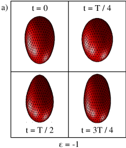
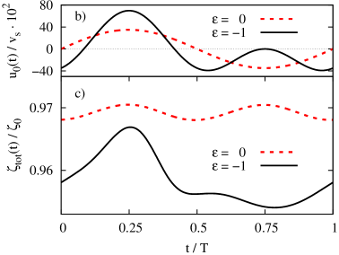
Figure 11: a) shows the capsule’s shape at different times in a shaken liquid with a non-symmetric liquid velocity, i.e., $u_{0}(t+T/2)\not=u_{0}(t)$, as shown by the solid line in b) and as given by equation (1) for $\varepsilon=-1.0$. In c) the drag coefficient $\zeta_{tot}(t)$ of the capsule is shown in units of $\zeta_{0}=6\pi\eta R$. In a sinusoidally shaken liquid, cf. dashed line in b), $\zeta_{tot}(t)$ is identical in both half periods. For a non-symmetrically shaken liquid also $\zeta_{tot}(t)$ is non-symmetric, cf. solid line and $\varepsilon=-1$, as well as the capsule shapes in a).

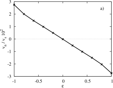
Figure 12: a) shows the mean-propulsion velocity $v_{n}$ of a homogeneous capsule as a function of the asymmetry parameter $\varepsilon$ of the shaking velocity in equation (1). For a sinusoidal shaking with $\varepsilon=0$ the capsule sinks. At sufficiently negative values $\varepsilon<0$ the capsule moves upwards and for $\varepsilon>0$ downwards. This allows to control the direction of $v_{n}$ via the time-dependence of liquid shaking. In b) $v_{n}$ is given as function of the amplitude $U$ of the shaking velocity. At low values of $U$ the shaking effect is weak and the capsule sinks. In the range $U\geq 450v_{s}$ the actuation induced by the shaking is stronger than the gravity and the capsule moves upwards.

In figure 11a) the shape of the capsule is shown during one period $T$ of the non-symmetric shaking velocity with $u_{0}(t+T/2)\not=u_{0}(t)$. For a sinusoidal shaking as displayed in figure 11b), i.e., $\varepsilon=0$ and $u_{0}(t)=-u_{0}(t+T/2)$, the capsule’s drag coefficient $\zeta_{tot}(t)$ (cf. A ) shown in figure 11c) is the same during both half periods of the shaking with $\zeta_{tot}(t)=\zeta_{tot}(t+T/2)$. In this case there is no mean actuation and the capsule just sediments due to gravity. If the liquid is shaken non-symmetrically with $\varepsilon\not=0$ the drag coefficient differs in both half periods, i.e., $\zeta_{tot}(t)\neq\zeta_{tot}(t+T/2)$. In this case the capsule is actuated by liquid shaking.

Figure 12a) shows how the mean velocity $v_{n}$ of the capsule depends on the asymmetry parameter $\varepsilon$ of the shaking velocity. At sufficient negative values of $\varepsilon\lesssim-0.01$ the upward oriented actuation overcomes gravity and we find a positive mean velocity $v_{n}$. Positive values of $\varepsilon$ enhance the sedimentation. Thus the direction of the mean capsule actuation can be controlled via the asymmetry parameter $\varepsilon$ of the shaking velocity. Note that the mean velocity induced by the shaking also depends on the period $T$.

Besides the asymmetry $\varepsilon$ also a sufficiently high amplitude $U$ of the shaking velocity is required to overcome gravity. Figure 12b) displays the mean velocity $v_{n}$ as a function of the amplitude $U$: At low values of $U$ the capsule sinks due to the gravity. For the chosen parameters one finds with $U=0$ the sedimentation velocity $v_{s}=0.19\frac{\mbox{mm}}{\mbox{s}}$. For $U\gtrsim 450v_{s}$ the mean velocity $v_{n}$ induced by liquid shaking is stronger than sedimentation and the capsule moves upwards for $\varepsilon=-1.0$. The Reynolds number used in figure 12b) is $0<$ Re $\lesssim 2$. Hence, the inertia induced actuation effect is found at small as well as at intermediate values of Re. The qualitative results are comparable to those found for the ring in the previous section in the limit of a vanishing Reynolds number, compare e.g., figure 10a) and figure 12b). The reason is that the requirements of the particle locomotion are the inertia of the particle and the time-dependent stokes drag, which is both included in the model of the bead-spring ring.

5 Summary and conclusions

We investigated a new kind of microswimmers, so-called passive swimmers. These microswimmers are soft particles with a mass density different from the liquid, which are driven by an oscillating background flow or a shaking of the liquid.

Previous studies focused on the propulsion of intrinsically asymmetric soft particles in sinusoidal liquid motion [11, 12]. With our extension to soft bead-spring tetrahedrons and to asymmetric, soft Janus capsules, we show that the inertia driven propulsion mechanism can even outweigh gravity. Moreover, we show that this novel inertia driven passive swimming mechanism works for the wider class of symmetric soft particles, such as capsules.

By a semi-analytical model calculation we cover the essential properties of the inertia driven propulsion mechanism in liquids shaken periodically with the velocity ${\bf u}_{0}(t+T)={\bf u}_{0}(t)$. It shows the following requirements: First, the mass densities of the particles and the liquid must be different. Secondly, the Stokes drag during both periods of the shaking with different directions must differ (e.g., due to a deformation). Thirdly, the shaking period $T$ has to be chosen in the order of magnitude of the relaxation time that the particles needs to adjust to the liquid velocity. The essential difference in the drag coefficient during both half periods is achieved by the asymmetry of the particle.

We suggest that this asymmetry can also be achieved by a non-symmetric shaking velocity with ${\bf u}_{0}(t+T/2)\not={\bf u}_{0}(t)$, as given for instance by equation (1), instead of the intrinsic particle asymmetry. Such a non-symmetric liquid shaking leads to a non-reciprocal particle deformation and Stokes drag.

This qualitative reasoning and the analytical considerations are verified and supported by simulations. We use symmetric and asymmetric bead spring models and complementary Lattice Boltzmann Simulations of realistic soft symmetric capsules and asymmetric Janus capsules. Asymmetric particles in a sinusoidally shaken fluid have two stable orientations and they exhibit therefore two directions of passive swimming, depending on the initial orientation. In contrast, for the wider class of symmetric particles in non-symmetrically shaken liquids the propulsion direction is determined by the shaking. Therefore the swimming direction can be selected by the engineered time-dependence of liquid shaking.

To provide examples of achievable propulsion velocities for symmetric and asymmetric Janus capsules we chose a realistic capsule size of about $10\,\mu$m and a stiffness of $8\cdot 10^{-4}~{}\frac{\mbox{N}}{\mbox{m}}$, which fits the values of common capsules [25, 43, 44]. A higher mass density for capsules than for the liquid can be achieved if salt is dissolved in the liquid inside the capsule [45], whereby water with dissolved salt can reach densities up to three times higher than pure water (without salt). Here we chose the mass density ratio $\rho_{caps}/\rho_{liquid}=2.0$ and the shaking frequency 10 kHz (see e.g., [46, 47, 48]) of the order of the inverse of velocity relaxation time of about $44\mu\mbox{s}$. For this choice of parameters and a maximal amplitude 0.5 $\frac{\mbox{m}}{\mbox{s}}$ of the liquid velocity one obtains for a symmetric capsule with in Lattice Boltzmann simulations an upward swim velocity of about 57 $\frac{\mbox{mm}}{\mbox{s}}$. For a Janus capsule one obtains for shaking-velocity amplitude 0.3 $\frac{\mbox{m}}{s}$ an upward swim velocity of about 15 $\frac{\mbox{mm}}{\mbox{s}}$.

Besides the possibility to engineer passive swimmers, the described effects have further applications: The inertia induced actuation may be exploited for separating particles with respect to their different mass and different elasticity (deformability). The separation of two kinds of soft particles with a different stiffness is achieved by choosing a shaking period that fits the shape relaxation time of one type of particles but not of the others. In this case one particle type is stronger actuated and can be accumulated for instance near one container wall. An example are biological cells. They have often a different density than water [49] or other carrier liquids. In addition the stiffness of cells is often an indicator of their health status [50, 51, 52]. In this case healthy cells may be separated for instance from malignant cells by non-symmetric liquid shaking. Our insights about inertia driven particle propulsion might also have impact on further systems studied at finite values of the Reynolds number [53, 54].

6 Acknowledgments

We acknowledge the support by the French-German University (Grant CFDA-Q1-14, program “Living fluids”).

Appendix A Dynamic Oseen tensor and drag coefficient

Dynamic Oseen tensor.

The liquid velocity ${\bf u}({\bf r}_{i})$ at the particle positions ${\bf r}_{i}$ includes the imposed homogeneous flow ${\bf u}_{0}$ as described by equation (1) and the flow disturbances caused by differences between the particle velocities ${\bf v}_{j}$ and the liquid velocity ${\bf u}_{0}({\bf r}_{j})$. For this we use the general solution of the linear part of the Navier-Stokes-equation $\rho_{f}\frac{\partial\mathbf{u}}{\partial t}=\eta\Delta\mathbf{u}-\nabla p+\mathbf{f}(\mathbf{r},t)$ for an arbitrary point-like force acting on the fluid. The solution of this problem with a point force $\mathbf{f}(\mathbf{r},t)=\mathbf{F}(t)\delta(r-r^{\prime})$ is given by [33]

$$\mathbf{u}_{\delta}(\mathbf{r}) = \frac{1}{\rho_{f}}\int_{0}^{t}dt^{\prime}\ \mathbf{H}({\mathbf{r}-\mathbf{r}^{\prime}},t^{\prime})\mathbf{F}(t^{\prime})\,,$$ (40)

$$\mathbf{H}(\mathbf{r}) = p(r,t)\mathbf{1}-q(r,t)\frac{\mathbf{r\otimes r}}{r^{2}}\,,$$ (41)

$$p(r,t) = \left(1+\frac{2\nu t}{r^{2}}\right)f(r,t)-\frac{g(r,t)}{r^{2}}\,,$$ (42)

$$q(r,t) = \left(1+\frac{6\nu t}{r^{2}}\right)f(r,t)-\frac{3g(r,t)}{r^{2}}\,,$$ (43)

$$f(r,t) = \frac{1}{(4\pi\nu t)^{3/2}}\exp\left[\frac{-r^{2}}{4\nu t}\right]\,,$$ (44)

$$g(r,t) = \frac{1}{4\pi r}\Phi\left[\frac{r}{(4\nu t)^{1/2}}\right]\,,$$ (45)

with $\nu=\frac{\eta}{\rho}$, the error function $\Phi$, the unit matrix $\mathbf{1}$ and the dyadic product $\otimes$. This allows to calculate the liquid velocity at a bead position $\mathbf{u}_{i}=\mathbf{u}(\mathbf{r}_{i})$,

$$\mathbf{u}_{i}=\mathbf{u}_{0}(t)-\frac{1}{\rho_{f}}\sum\limits_{j\neq i}\int\limits_{0}^{t}dt^{\prime}\ \mathbf{H}_{i,j}(t^{\prime})\cdot\mathbf{F}_{j}^{(1)}(t^{\prime})\\$$ (46)

with $\mathbf{H}_{i,j}(t)=\mathbf{H}({\mathbf{r}_{i}-\mathbf{r}_{j}},t)$. This velocity is composed of the homogeneous background flow and the liquid velocity changes caused by the differences between the particle velocities and the flow ${\bf u}_{0}$, which are induced by the forces ${\bf F}_{j}^{(1)}$ given in section 2.2.

Determination of the drag coefficient.

To calculate the drag $\zeta_{tot}(t)$, we follow the procedure given in [55, 56, 57]. For this, we use the positions of the beads/nodes on the particle surface obtained by simulations. The drag at time $t$ is determined by assuming a fixed shape which implies a constant velocity $\mathbf{v}_{i}=\mathbf{v}=v\hat{\mathbf{e}}_{y}$ on each bead/node. We calculate the forces via

$$\mathbf{v}_{i}=\sum_{j}\mathbf{H}_{i,j}\cdot\mathbf{F}^{(P)}_{j},$$ (47)

where

$$\mathbf{H}_{i,j}=\left\{\begin{array}[]{l}\mathbf{O}(\mathbf{r}_{i}-\mathbf{r}_{j}),\\ \frac{1}{\zeta}_{b}\mathbf{1}\end{array}\right.$$ (48)

is the mobility matrix including the hydrodynamic interaction between particle $\mathbf{r}_{i}$ and $\mathbf{r}_{j}$ described by the Oseen tensor $\mathbf{O}(\mathbf{r})=\frac{1}{8\pi\eta r}\left(\mathbf{1}+\frac{\mathbf{r}\otimes\mathbf{r}}{r^{2}}\right)$. The drag finally follows with

$$\mathbf{F}_{tot}=\sum_{j}\mathbf{F}_{j}=\zeta_{tot}\mathbf{v}.$$ (49)

The values $\zeta_{1}$ and $\zeta_{2}$ (used in equation (29)) are chosen as the maximal value during the first or the second halve period, respectively.

Appendix B Tetrahedron consisting of beads with different mass

Here we investigate the effects of the mass inhomogeneity on the propulsion velocity of a tetrahedron. If all beads of a tetrahedron have the same mass density, the upward oriented tetrahedron ($\blacktriangle$) and the downward oriented one ($\blacktriangledown$) are both stable. By changing the mass density of one of the four beads then one of both orientations with respect to the gravitational field is preferred, similar as in reference [12]. For example, if the tetrahedron sinks (without liquid shaking) the lighter bead points upwards after a certain time. For this orientation we investigate the effect of a inhomogeneous mass density on the propulsion velocity.

We introduce the density ratio $\alpha$ between one and the other three beads, i.e., $\rho_{1}=\alpha\rho_{2,3,4}$, and keep the mean density $\bar{\rho}$ constant:

$$\overline{\rho} = \frac{1}{N}\sum\limits_{i=1}^{N}\rho_{i}\,,$$ (50)

$$\rho_{1} = \alpha\rho_{2},\ \rho_{2}=\rho_{3}=\rho_{4}\,.$$ (51)

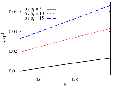
Figure 13: The left part shows the mean propulsion velocity of the tetrahedron for different mass-density ratios $\bar{\rho}/\rho_{f}$ as function of the density ratio $\alpha$ and the right part the amplitude of the shape deformation $\bar{A}$ as defined in equation (39).

Figure 13 shows the mean velocity $v_{n}$ of the tetrahedron and the amplitude of the shape deformation $\bar{A}$ (defined in equation (39)) as a function of the mass-density ratio $\alpha$ simulated with the Maxey Riley equations. The tetrahedron moves slower with an increasing difference of the densities of the beads, which can be explained as follows. A lighter bead can follow the heavier ones easily and thus the lighter bead moves more in phase with the heavy beads than a bead of the same mass density. This results in smaller spring deformation and in a lower deformation amplitude $\bar{A}$, cf. figure 13. A smaller amplitude $\bar{A}$ leads to smaller temporal changes of the drag coefficient $\zeta_{tot}$ and therefore to slower mean velocity.

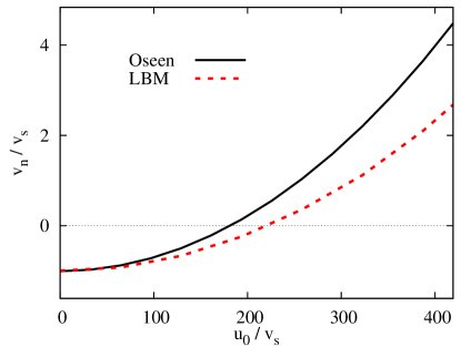
Figure 14: The mean propulsion velocity of a tetrahedron is shown for $\alpha=0.6$ as a function of the amplitude $U$ of the liquid velocity, obtained by simulations of the Maxey-Riley equations and Lattice Boltzmann simulations.

So far we have used the Maxey and Riley equations and the dynamic Oseen tensor, i.e., we have neglected effects of a finite Reynolds number. Here we compare the results with Lattice Boltzmann simulations of the full Navier-Stokes equation with the tetrahedron. Figure 14 shows the mean velocity of a tetrahedron with $\alpha=0.6$ as function of the amplitude $U$ of the shaking velocity. Both methods show that the mean velocity increases continuously with the amplitude $U$. Furthermore both simulations show that at low values of $U$ the tetrahedron sinks and above a critical value of $U$ the tetrahedron rises against gravity. Thus the numerical methods agree qualitatively. This means the LBM simulations, taking effects of a finite Reynolds number into account, and the Maxey and Riley equations including the dynamic Oseen tensor in the limit $Re=0$ describe inertia induced propulsion of the tetrahedron. This confirms that the mean velocity is the result of the temporal change of the drag coefficient $\zeta_{tot}(t)$ and a finite Reynolds number just modifies this result quantitatively.

Appendix C Discussion of the sign of the mean velocity

The mean velocity $v_{n}$ of the particle is given by equations (34) and (35) in the main text as follows

$$\Gamma = \frac{(\zeta_{1}-\zeta_{2})(M-M_{f})}{(\omega^{2}M^{2}+\zeta_{2}^{2})(\omega^{2}M^{2}+\zeta_{1}^{2})}\,,$$

$$v_{n} = \frac{\int_{0}^{T}v(t)dt}{T}$$

$$= \Gamma\ \frac{U\omega^{2}M}{2\zeta_{1}\zeta_{2}\pi}\left[(\zeta_{1}+\zeta_{2})(\zeta_{1}\zeta_{2}+\omega^{2}M^{2})\right.$$

$$\qquad+\left.(\zeta_{1}-\zeta_{2})(\omega^{2}M^{2}-\zeta_{1}\zeta_{2})\frac{\exp\frac{\zeta_{2}\pi}{\omega M}-\exp\frac{\zeta_{1}\pi}{\omega M}}{\exp\frac{\pi(\zeta_{1}+\zeta_{2})}{\omega M}-1}\right]\,.$$

We show here that the sign of the mean velocity is determined by $\Gamma$ because all other factors in the equation of $v_{n}$ (equation (35)) are positive.

The factor $\frac{U\omega^{2}M}{2\zeta_{1}\zeta_{2}\pi}$ is positive because we assume $U>0$. We define furthermore

$$A=(\zeta_{1}+\zeta_{2})(\zeta_{1}\zeta_{2}+\omega^{2}M^{2})$$ (52)

$$B=(\zeta_{1}-\zeta_{2})(\omega^{2}M^{2}-\zeta_{1}\zeta_{2})\frac{\exp\frac{\zeta_{2}\pi}{\omega M}-\exp\frac{\zeta_{1}\pi}{\omega M}}{\exp\frac{\pi(\zeta_{1}+\zeta_{2})}{\omega M}-1}$$ (53)

which leads to

$$v_{n}=\Gamma\ \frac{U\omega^{2}M}{2\zeta_{1}\zeta_{2}\pi}\left[A+B\right]\,.$$

It is trivial that $A$ is positive. We demonstrate now $A+B>0$ by showing that $|A|>|B|$. We compare the absolute values of $A$ and by $B$ for each factor. It is clear that

$$|\zeta_{1}+\zeta_{2}|>|\zeta_{1}-\zeta_{2}|\,,$$ (54)

$$|\zeta_{1}\zeta_{2}+\omega^{2}M^{2}|>|\omega^{2}M^{2}-\zeta_{1}\zeta_{2}|\,.$$ (55)

To show

$$1\geq\left|\frac{\exp\frac{\zeta_{2}\pi}{\omega M}-\exp\frac{\zeta_{1}\pi}{\omega M}}{\exp\frac{\pi(\zeta_{1}+\zeta_{2})}{\omega M}-1}\right|$$ (56)

we define

$$a_{1,2} = \frac{\zeta_{1,2}\pi}{\omega M}>0\,,$$ (57)

$$f(a_{1},a_{2}) = \frac{\exp a_{2}-\exp a_{1}}{\exp(a_{1}+a_{2})-1}\,.$$ (58)

The function $f$ has the following properties: it increases monotonously with $a_{2}$ and decreases monotonously with $a_{1}$. Furthermore it is

$$f(0,a_{2})=1\,,$$ (59)

$$\lim_{a_{1}\to\infty}f(a_{1},a_{2})=-\exp{(-a_{2})}\,,$$ (60)

$$f(a_{1},0)=-1\,,$$ (61)

$$\lim_{a_{2}\to\infty}f(a_{1},a_{2})=\exp{(-a_{1})}\,.$$ (62)

With $a_{1,2}\geq 0$ follows

$$-1\leq f(a_{1},a_{2})\leq 1\,,$$ (63)

$$|f(a_{1},a_{2})|<1\,.$$ (64)

The equations (54), (55), (64) lead to $|A|>|B|$ and with $A>0$ follows $A+B>0$. Therefore we get for eq. (equation (35)

$$v_{n} = \Gamma\ \underbrace{\frac{U\omega^{2}M}{2\zeta_{1}\zeta_{2}\pi}}_{>0}$$

$$\underbrace{\left[(\zeta_{1}+\zeta_{2})(\zeta_{1}\zeta_{2}+\omega^{2}M^{2})(\zeta_{1}-\zeta_{2})(\omega^{2}M^{2}-\zeta_{1}\zeta_{2})\frac{\exp\frac{\zeta_{2}\pi}{\omega M}-\exp\frac{\zeta_{1}\pi}{\omega M}}{\exp\frac{\pi(\zeta_{1}+\zeta_{2})}{\omega M}-1}\right]}_{>0}$$

which means the sign of $v_{n}$, i.e. the direction of the mean velocity is determined by the factor $\Gamma$ if $U>0$ is assumed.

References

- [1] Lauga E and Goldstein R E 2012 Physics Today 65 30
- [2] Lauga E and Powers T R 2009 Phys. Rep. 72 096601
- [3] Guasto J S, Rusconi R and Stocker R 2012 Annu. Rev. Fluid Mech. 44 373
- [4] Bechinger C, Leonardo R D, Löwen H, Reichardt C, Volpe G and Volpe G 2016 Rev. Mod. Phys. 88 045006
- [5] Lauga E 2016 Annu. Rev. Fluid Mech. 48 105
- [6] Squires T M and Quake S R 2005 Rev. Mod. Phys. 77 978
- [7] Sackmann E K, Fulton A L and Beebe D L 2014 Nature 507 181
- [8] Dahl J B, Lin J M G, Muller S J and Kumar S 2015 Ann. Rev. Chem. Biomol. Eng. 6 293
- [9] Amini H, Lee W and Carlo D D 2014 Lap Chip 14 2739
- [10] Secomb T W 2017 Annu. Rev. Fluid Mech. 49 443
- [11] Jo I, Huang Y, Zimmermann W and Kanso E 2016 Phys. Rev. E 94 063116
- [12] Morita T, Omori T and Ishikawa T 2018 Phys. Rev. E 98 023108
- [13] Goldstein R E 2015 Annu. Rev. Fluid Mech. 47 343
- [14] Wu H, Thiébaud M, Hu W F, Farutin A, Rafaï S, Lai M C, Peyla P and Misbah C 2015 Phys. Rev. E 92 050701
- [15] Wu H, Farutin A, Hu W F, Thiébaud M, Rafaï S, Peyla P, Lai M C and Misbah C 2016 Soft Matter 12 7470
- [16] Farutin A, Rafaï S, Dysthe D K, Duperray A, Peyla P and Misbah C 2013 Phys. Rev. Lett. 111 228102
- [17] Purcell E M 1977 Am. J. Phys. 45 3
- [18] Laumann M, Bauknecht P, Gekle S, Kienle D and Zimmermann W 2017 EPL 117 44001
- [19] Olla P 2010 Phys. Rev. E 82 015302(R)
- [20] Leal L G 1980 Annu. Rev. Fluid Mech. 12 435
- [21] Mandal S, Bandopadhyay A and Chakraborty S 2015 Phys. Rev. E 92 023002
- [22] Kaoui B, Ristow G H, Cantat I, Misbah C and Zimmermann W 2008 Phys. Rev. E 77 021903
- [23] Coupier G, Kaoui B, Podgorski T and Misbah C 2008 Phys. Fluids 20 111702
- [24] Doddi S K and Bagchi P 2008 Int. J. Multiphase Flow 34 966
- [25] Chen L, An H Z and Doyle P S 2015 Langmuir 31 9228
- [26] Klosta D, Baldwin K A, Baldwin R J A, Hill R J A, Bowley R M and Swift M R 2015 Phys. Rev. Lett. 115 248102
- [27] Maxey M R and Riley J J 1983 Phys. Fluids 26 883
- [28] Krueger T, Varnik F and Raabe D 2011 Comput. Math. Appl. 61 3485
- [29] Ramanjan S and Pozrikidis C 1998 J. Fluid Mech. 361 117
- [30] Barthès-Biesel D 2016 Annu. Rev. Fluid Mech. 48 25
- [31] G Gompper and DM Kroll 1996 J. Phys. I France 6 1305
- [32] Krueger T, Gross M, Raabe D and Varnik F 2013 Soft Matter 9 9008
- [33] Español P, Rubio M A and Zúñiga I 1995 Phys. Rev. E 51 803
- [34] Aidun C K and Clausen J R Annu. Rev. Fluid. Mech.
- [35] Aidun C K, Lu Y and Ding E J 1998 J. Fluid Mech. 373 287
- [36] d’Humières D, Ginzburg I, Krafczyk M, Lallemand P and Luo L S 2002 Phil. Trans. R. Soc. Lond. A 360 437
- [37] Ladd A J C 1994 J. Fluid Mech. 271 285
- [38] Guo Z, Zheng C and Shi B 2002 Phys. Rev. E 65 046308
- [39] Ladd A J C and Verberg R 2001 J. Stat. Phys. 104 1191
- [40] Shao J Y and Shu C 2015 Int. J. Numer. Methods Fluids 77 526
- [41] Premnath K N and Abraham J 2007 J. Comput. Phys. 224 539
- [42] Peskin C S 2002 Acta Numer. 11 479
- [43] Sun H, Wong E H H, Yan Y, Cui J, Dai Q, Guo J, Qiao G G and Caruso F 2015 Chem. Sci. 6 3505
- [44] Amstad E 2017 CHIMIA 71 334
- [45] Koroznikova L, Klutke C, McKnight S and Hall S 2008 J. S. Afr. Inst. Min. Metall. 108 25
- [46] Gerlach T, Schuenemann M and Wurmus H 1995 J. Micromech. Microeng. 5 199
- [47] Nabavi M and Mongeau L 2009 Microfluid. Nanofluid. 7 669
- [48] Roberts D C, Li H, Steyn J, Turner K T, Mlcak R, Saggere L, Spearing S, Schmidt M A and Hagood N W 2002 Sens. Actuators, A 97-98 620
- [49] Milo R and Phillips R 2016 Cell biology by the numbers (New York, NY: Garland Science)
- [50] Karimi A, Yazdi S and Ardekani A M 2013 Biomicrofluidics 7 021501
- [51] Cross S E, Jin Y S, Rao J and Gimzewski J K 2007 Nat. Nanotechnol. 2 780
- [52] Guck J, Schinkinger S, Lincoln B, Wottawah F, Ebert S, Romeyke M, Lenz D, Erickson H M, Ananthakrishnan R, Mitchell D, Käs J, Ulvick S and Bilby C 2005 Biophys. J. 88 3689
- [53] Sorokin V S, Blekhmann I I and Vasilkow V B 2012 Nonlinear Dyn. 67 147
- [54] Scholz C, Jahanshai S, Ldov A and Löwen H 2018 Nature Comm. 9 5156
- [55] Dhont J K G 1996 An Introduction to dynamics of colloids (Amsterdam: Elsevier)
- [56] Doi M and Edwards S F 1986 The Theory of Polymer Dynamics (Oxford: Clarendon Press)
- [57] Leal L G 2007 Advanced Transport Phenomena (Cambridge: Cambridge University Press)