On the uniqueness of Gibbs measure in the Potts model on a Cayley tree with external field

Abstract.

The paper concerns the $q$-state Potts model (i.e., with spin values in $\{1,\dots,q\}$) on a Cayley tree $\mathbb{T}^{k}$ of degree $k\geq 2$ (i.e., with $k+1$ edges emanating from each vertex) in an external (possibly random) field. We construct the so-called splitting Gibbs measures (SGM) using generalized boundary conditions on a sequence of expanding balls, subject to a suitable compatibility criterion. Hence, the problem of existence/uniqueness of SGM is reduced to solvability of the corresponding functional equation on the tree. In particular, we introduce the notion of translation-invariant SGMs and prove a novel criterion of translation invariance. Assuming a ferromagnetic nearest-neighbour spin-spin interaction, we obtain various sufficient conditions for uniqueness. For a model with constant external field, we provide in-depth analysis of uniqueness vs. non-uniqueness in the subclass of completely homogeneous SGMs by identifying the phase diagrams on the “temperature–field” plane for different values of the parameters $q$ and $k$. In a few particular cases (e.g., $q=2$ or $k=2$), the maximal number of completely homogeneous SGMs in this model is shown to be $2^{q}-1$, and we make a conjecture (supported by computer calculations) that this bound is valid for all $q\geq 2$ and $k\geq 2$.

1. Introduction

1.1. Background and motivation

The Potts model was introduced by R. B. Potts [43] as a lattice system with $q\geq 2$ spin states and nearest-neighbour interaction, aiming to generalize the Kramers–Wannier duality [28] of the Ising model ($q=2$). Since then, it has become the darling of statistical mechanics, both for physicists and mathematicians [4, 64], as one of few “exactly soluble” (or at least tractable) models demonstrating a phase transition [11, 15, 16, 27, 31, 35]. Due to its intuitive appeal to describe multistate systems, combined with a rich structure of inner symmetries, the Potts model has been quickly picked up by a host of research in diverse areas, such as probability [25], algebra [33], graph theory [5], conformally invariant scaling limits [46, 54], computer science [18], statistics [23, 39], biology [24], medicine [58, 59], sociology [53, 55], financial engineering [45, 60], computational algorithms [10, 17], technological processes [52, 62], and many more.

Much of this modelling has involved interacting spin system on graphs. In this context, tree-like graphs are especially attractive for the analysis due to their recursive structure and the lack of circuits. In particular, regular trees (known as Cayley trees or Bethe lattices [6]) have become a standard trial template for various models of statistical physics (see, e.g., [1, 2, 3, 34, 37, 61, 63]), which are interesting in their own right but also provide useful insights into (harder) models in more realistic spaces (such as lattices $\mathbb{Z}^{d}$) as their “infinite-dimensional” approximation [4, Chapter 4]. On the other hand, the use of Cayley trees is often motivated by the applications, such as information flows [38] and reconstruction algorithms on networks [15, 36], DNA strands and Holliday junctions [48], evolution of genetic data and phylogenetics [14], bacterial growth and fire forest models [12], or computational complexity on graphs [18]. Crucially, the criticality in such models is governed by phase transitions in the underlying spin systems.

It should be stressed, however, that the Cayley tree is distinctly different from finite-dimensional lattices, in that the ratio of the number of boundary vertices to the number of interior vertices in a large finite subset of the tree does not vanish in the thermodynamic limit. For example, if $k\geq 2$ is the degree of the tree (i.e., each vertex has $k+1$ neighbours), $V_{n}$ is a “ball” of radius $n$ (centred at some point $x_{\circ}$) and $\partial V_{n}=V_{n+1}\setminus V_{n}$ is the boundary “sphere”, then

$$\frac{|\partial V_{n}|}{|V_{n}|}=\frac{(k+1)\mbox{$\>\!$}k^{n}}{1+(k+1)(k^{n}-1)/(k-1)}\to k-1\geq 1,\qquad n\to\infty.$$

Therefore, the remote boundary may be expected to have a very strong influence on spins located deep inside the graph, which in turn pinpoints a rich and complex picture of phase transitions, including the number of possible pure phases of the system as a function of temperature.

Mathematical foundations of random fields on Cayley trees were laid by Preston [44] and Spitzer [57], followed by an extensive analysis of Gibbs measures and phase transitions (see Georgii [22, Chapter 12] and Rozikov [47], including historical remarks and further bibliography). The Ising model on a Cayley tree has been studied in most detail (see [47, Chapter 2] for a review). In particular, Bleher et al. [8] described the phase diagram of a ferromagnetic Ising model in the presence of an external random field. Using physical argumentation, Peruggi et al. [41, 42] considered the Potts model on a Cayley tree (both ferromagnetic and antiferromagnetic) with a (constant) external field, and discussed the “order/disorder” transitions (cf. [15, 18]).

In the present paper, we consider a similar (ferromagnetic) model but we are primarily concerned with more general “uniqueness/non-uniqueness” transitions. We choose to work with the so-called splitting Gibbs measures (SGM), which are conveniently defined in the thermodynamic limit using generalized boundary conditions (GBC). To be consistent, permissible GBC fields must satisfy a certain functional equation, which can then be used as a tool to identify the number of solutions. In this approach, it is crucial that any extremal Gibbs measure is SGM, and so the problem of uniqueness is reduced to that in the SGM class.

Külske et al. [30] described the full set of completely homogeneous SGMs for the $q$-state Potts model on a Cayley tree with zero external field; in particular, it was shown that, at sufficiently low temperatures, their number is $2^{q}-1$. Recently, Külske and Rozikov [29] found some regions for the temperature parameter ensuring that a given completely homogeneous SGM is extreme/non-extreme; in particular, there exists a temperature interval in which there are at least $2^{q-1}+q$ extreme SGMs. In contrast, in the antiferromagnetic Potts model on a tree, a completely homogeneous SGM is unique at all temperatures and for any field (see [47, Section 5.2.1]).

1.2. Set-up

We start by summarizing the basic concepts for Gibbs measures on a Cayley tree, and also fix some notation.

1.2.1. Cayley tree

Let $\mathbb{T}^{k}$ be a (homogeneous) Cayley tree of degree $k\geq 2$, that is, an infinite connected cycle-free (undirected) regular graph with each vertex incident to $k+1$ edges. For example, $\mathbb{T}^{1}=\mathbb{Z}$. Denote by $V=\{x\}$ the set of the vertices of the tree and by $E=\{\langle x,y\rangle\}$ the set of its (non-oriented) edges connecting pairs of neighbouring vertices. The natural distance $d(x,y)$ on $\mathbb{T}^{k}$ is defined as the number of edges on the unique path connecting vertices $x,y\in V$. In particular, $\langle x,y\rangle\in E$ whenever $d(x,y)=1$. A (non-empty) set $\varLambda\subset V$ is called connected if for any $x,y\in\varLambda$ the path connecting $x$ and $y$ lies in $\varLambda$. We denote the complement of $\varLambda$ by $\varLambda^{c}:=V\setminus\varLambda$ and its boundary by $\partial\varLambda:=\{x\in\varLambda^{c}\colon\exists\mbox{$\>\!$}y\in\varLambda,\ d(x,y)=1\}$, and we write $\bar{\varLambda}=\varLambda\cup\partial\varLambda$. The subset of edges in $\varLambda$ is denoted $E_{\varLambda}:=\{\langle x,y\rangle\in E\colon x,y\in\varLambda\}$.

Fix a vertex $x_{\circ}\mbox{$\;\!\!$}\in V$, interpreted as the root of the tree. We say that $y\in V$ is a direct successor of $x\in V$ if $x$ is the penultimate vertex on the unique path leading from the root $x_{\circ}$ to the vertex $y$; that is, $d(x_{\circ},y)=d(x_{\circ},x)+1$ and $d(x,y)=1$. The set of all direct successors of $x\in V$ is denoted $S(x)$. It is convenient to work with the family of the radial subsets centred at $x_{\circ}$, defined for $n\in\mathbb{N}_{0}:=\{0\}\cup\mathbb{N}$ by

$$V_{n}:=\{x\in V\colon d(x_{\circ},x)\leq n\},\qquad W_{n}:=\{x\in V\colon d(x_{\circ},x)=n\},$$

interpreted as the “ball” and “sphere”, respectively, of radius $n$ centred at the root $x_{\circ}$. Clearly, $\partial V_{n}=W_{n+1}$. Note that if $x\in W_{n}$ then $S(x)=\{y\in W_{n+1}\colon d(x,y)=1\}$. In the special case $x=x_{\circ}$ we have $S(x_{\circ})=W_{1}$. For short, we set $E_{n}:=E_{V_{n}}$.

Remark 1.1.

Note that the sequence of balls $(V_{n})$ ($n\in\mathbb{N}_{0}$) is cofinal (see [22, Section 1.2, page 17]), that is, any finite subset $\varLambda\subset V$ is contained in some $V_{n}$.

1.2.2. The Potts model and Gibbs measures

In the $q$-state Potts model, the spin at each vertex $x\in V$ can take values in the set $\varPhi:=\{1,\dots,q\}$. Thus, the spin configuration on $V$ is a function $\sigma\colon V\!\to\varPhi$ and the set of all configurations is $\varPhi^{V}$ . For a subset $\varLambda\subset V$, we denote by $\sigma_{\mbox{$\;\!\!$}\varLambda}\colon\varLambda\to\varPhi$ the restriction of configuration $\sigma$ to $\varLambda$,

$$\sigma_{\mbox{$\;\!\!$}\varLambda}(x):=\sigma(x),\qquad x\in\varLambda.$$

The Potts model with a nearest-neighbour interaction kernel $\{J_{xy}\}_{x,\mbox{$\>\!$}y\mbox{$\>\!$}\in\mbox{$\>\!$}V}$ (i.e., such that $J_{xy}=J_{yx}$ and $J_{xy}=0$ if $d(x,y)\neq 1$) is defined by the formal Hamiltonian

$$H(\sigma)=-\sum_{\langle x,\mbox{$\>\!$}y\rangle\in E}\!J_{xy}\mbox{$\;\!$}\delta_{\sigma(x),\mbox{$\>\!$}\sigma(y)}-\sum_{x\in V}\xi_{\sigma(x)}(x),\qquad\sigma\in\varPhi^{V},$$ (1.1)

where $\delta_{ij}$ is the Kronecker delta symbol (i.e., $\delta_{ij}=1$ if $i=j$ and $\delta_{ij}=0$ otherwise), and $\boldsymbol{\xi}(x)=(\xi_{1}(x),\dots,\allowbreak\xi_{q}(x))\allowbreak\in\mathbb{R}^{q}$ is the external (possibly random) field. According to (1.1), the spin-spin interaction is activated only when the neighbouring spins are equal, whereas the additive contribution of the external field is provided, at each vertex $x\in V$, by the component of the vector $\boldsymbol{\xi}(x)$ corresponding to the spin value $\sigma(x)$.

For each finite subset $\varLambda\subset V$ ($\varLambda\neq\varnothing$) and any fixed subconfiguration $\eta\in\varPhi^{\varLambda^{c}}$ (called the configurational boundary condition), the Gibbs distribution $\gamma^{\eta}_{\mbox{$\;\!\!$}\varLambda}$ is a probability measure in $\varPhi^{\varLambda}$ defined by the formula

$$\gamma^{\eta}_{\mbox{$\;\!\!$}\varLambda}(\varsigma)=\frac{1}{Z^{\eta}_{\mbox{$\;\!\!$}\varLambda}(\beta)}\exp\biggl{\{}-\beta H_{\mbox{$\;\!\!$}\varLambda}(\varsigma)+\beta\sum_{x\in\varLambda}\sum_{y\in\varLambda_{\vphantom{t}}^{c}}\!J_{xy}\mbox{$\;\!$}\delta_{\varsigma(x),\mbox{$\>\!$}\eta(y)}\biggr{\}},\qquad\varsigma\in\varPhi^{\varLambda},$$ (1.2)

where $\beta\in(0,\infty)$ is a parameter (having the meaning of inverse temperature), $H_{\mbox{$\;\!\!$}\varLambda}$ is the restriction of the Hamiltonian (1.1) to subconfigurations in $\varLambda$,

$$H_{\mbox{$\;\!\!$}\varLambda}(\varsigma)=-\sum_{\langle x,\mbox{$\>\!$}y\rangle\in E_{\varLambda}}\!\!J_{xy}\mbox{$\;\!$}\delta_{\varsigma(x),\mbox{$\>\!$}\varsigma(y)}-\sum_{x\in\varLambda}\xi_{\varsigma(x)}(x),\qquad\varsigma\in\varPhi^{\varLambda},$$ (1.3)

and $Z^{\eta}_{\mbox{$\;\!\!$}\varLambda}(\beta)$ is the normalizing constant (often called the canonical partition function),

$$Z^{\eta}_{\mbox{$\;\!\!$}\varLambda}(\beta)=\sum_{\varsigma\in\varPhi^{\varLambda}}\exp\mbox{$\;\!\!$}\Biggl{\{}-\beta H_{\mbox{$\;\!\!$}\varLambda}(\varsigma)+\beta\sum_{x\in\varLambda}\sum_{y\in\varLambda_{\vphantom{t}}^{c}}J_{xy}\mbox{$\;\!$}\delta_{\varsigma(x),\mbox{$\>\!$}\eta(y)}\Biggr{\}}.$$

Due to the nearest-neighbour interaction, formula (1.2) can be rewritten as

$$\gamma^{\eta}_{\mbox{$\;\!\!$}\varLambda}(\varsigma)=\frac{1}{Z^{\eta}_{\mbox{$\;\!\!$}\varLambda}(\beta)}\exp\mbox{$\;\!\!$}\Biggl{\{}-\beta H_{\varLambda}(\varsigma)+\beta\sum_{x\in\varLambda}\sum_{y\in\partial\varLambda}\!J_{xy}\mbox{$\;\!$}\delta_{\varsigma(x),\mbox{$\>\!$}\eta(y)}\Biggr{\}},\qquad\varsigma\in\varPhi^{\varLambda}.$$ (1.4)

Finally, a measure $\mu=\mu_{\beta,\mbox{$\>\!$}\xi}$ on $\varPhi^{V}$ is called a Gibbs measure if, for any non-empty finite set $\varLambda\subset V$ and any $\eta\in\varPhi^{\varLambda^{c}}\!$,

$$\mu(\sigma_{\mbox{$\;\!\!$}\varLambda}=\varsigma\mbox{$\;\!$}|\mbox{$\;\!$}\sigma_{\mbox{$\;\!\!$}\varLambda^{c}}\mbox{$\;\!\!$}=\eta)\equiv\gamma_{\mbox{$\;\!\!$}\varLambda}^{\eta}\mbox{$\;\!\!$}(\varsigma),\qquad\varsigma\in\varPhi^{\varLambda}.$$ (1.5)

1.2.3. SGM construction

It is convenient to construct Gibbs measures on the Cayley tree $\mathbb{T}^{k}$ using a version of Gibbs distributions on the balls $(V_{n})$ defined via auxiliary fields encapsulating the interaction with the exterior of the balls. More precisely, for a vector field $V\ni x\mapsto\boldsymbol{h}(x)=(h_{1}(x),\dots,h_{q}(x))\in\mathbb{R}^{q}$ and each $n\in\mathbb{N}_{0}$, define a probability measure in $V_{n}$ by the formula

$$\mu^{h}_{n}(\sigma_{n})=\frac{1}{Z_{n}}\exp\left\{-\beta H_{n}(\sigma_{n})+\beta\!\sum_{x\in W_{n}}\!h_{\sigma_{n}(x)}(x)\right\},\qquad\sigma_{n}\in\varPhi^{V_{n}},$$ (1.6)

where $Z_{n}=Z_{n}(\beta,\boldsymbol{h})$ is the normalizing factor and $H_{n}:=H_{V_{n}}$, that is (see (1.3)),

$$H_{n}(\sigma_{n})=-\sum_{\langle x,y\rangle\in E_{n}}\!\!J_{xy}\mbox{$\;\!$}\delta_{\sigma_{n}(x),\mbox{$\>\!$}\sigma_{n}(y)}-\sum_{x\in V_{n}}\xi_{\sigma_{n}(x)}(x),\qquad\sigma_{n}\in\varPhi^{V_{n}}.$$ (1.7)

The vector field $\{\boldsymbol{h}(x)\}_{x\in V}$ in (1.6) is called generalized boundary conditions (GBC).

We say that the probability distributions (1.6) are compatible (and the intrinsic GBC $\{\boldsymbol{h}(x)\}$ are permissible) if for each $n\in\mathbb{N}_{0}$ the following identity holds,

$$\sum_{\omega\in\varPhi^{W_{n+1}}}\!\mu^{h}_{n+1}(\sigma_{n}\mbox{$\;\!\!$}\mbox{$\>\!\!$}\vee\omega)\equiv\mu^{h}_{n}(\sigma),\qquad\sigma_{n}\in\varPhi^{V_{n}},$$ (1.8)

where the symbol $\vee$ stands for concatenation of subconfigurations. A criterion for permissibility of GBC is provided by Theorem 2.1 (see Section 2.1 below). By Kolmogorov’s extension theorem (see, e.g., [56, Chapter II, § 3, Theorem 4, page 167]), the compatibility condition (1.8) ensures that there exists a unique measure $\mu^{h}=\mu^{h}_{\beta,\mbox{$\>\!$}\xi}$ on $\varPhi^{V}$ such that, for all $n\in\mathbb{N}_{0}$,

$$\mu^{h}(\sigma_{V_{n}}\mbox{$\;\!\!$}\mbox{$\>\!\!$}=\sigma_{n})\equiv\mu^{h}_{n}(\sigma_{n}),\qquad\sigma_{n}\in\varPhi^{V_{n}},$$ (1.9)

or more explicitly (substituting (1.6)),

$$\mu^{h}(\sigma_{V_{n}}\!=\sigma_{n})=\frac{1}{Z_{n}}\exp\left\{-\beta H_{n}(\sigma_{n})+\beta\sum_{x\in W_{n}}h_{\sigma_{n}(x)}(x)\right\},\qquad\sigma_{n}\in\varPhi^{V_{n}}.$$ (1.10)

It is easy to show that $\mu^{h}$ so defined is a Gibbs measure (see (1.5)); since the family $(V_{n})$ is cofinal (see Remark 1.1), according to a standard result [22, Remark (1.24), page 17] it suffices to check that, for each $n\in\mathbb{N}_{0}$ and any $\eta\in\varPhi^{V_{n\vphantom{t}}^{c}}$,

$$\mu^{h}(\sigma_{V_{n}}\mbox{$\;\!\!$}\mbox{$\>\!\!$}=\sigma_{n}\mbox{$\>\!$}|\mbox{$\;\!$}\sigma_{V_{n\vphantom{t}}^{c}}=\eta)\equiv\gamma_{n}^{\eta}\mbox{$\;\!\!$}(\sigma_{n}),\qquad\sigma_{n}\in\varPhi^{V_{n}},$$ (1.11)

where $\gamma^{\eta}_{n}$ is the Gibbs distribution in $V_{n}$ with configurational boundary condition $\eta$ (cf. (1.2)). Indeed, denote $\omega:=\eta_{\mbox{$\>\!$}W_{n+1}\mbox{$\>\!\!$}}\in\varPhi^{W_{n+1}}\mbox{$\>\!\!$}$, then, due to the nearest-neighbour interaction in the Hamiltonian (1.1) and according to (1.9), we have

$$\mu^{h}(\sigma_{V_{n}}\mbox{$\;\!\!$}\mbox{$\>\!\!$}=\sigma_{n}\mbox{$\>\!$}|\mbox{$\;\!$}\sigma_{V_{n\vphantom{t}}^{c}}=\eta) =\mu^{h}(\sigma_{V_{n}}\mbox{$\;\!\!$}\mbox{$\>\!\!$}=\sigma_{n}\mbox{$\>\!$}|\mbox{$\;\!$}\sigma_{W_{n+1}}\mbox{$\;\!\!$}\mbox{$\>\!\!$}=\omega)$$

$$=\frac{\mu^{h}(\sigma_{V_{n+1}\mbox{$\>\!\!$}}\mbox{$\>\!\!$}=\sigma_{n}\mbox{$\>\!\!$}\vee\omega)}{\mu^{h}(\sigma_{W_{n+1}}\mbox{$\;\!\!$}\mbox{$\>\!\!$}=\omega)}$$

$$=\frac{\mu^{h}_{n+1}(\sigma_{n}\mbox{$\>\!\!$}\vee\omega)}{\mu^{h}_{n+1}(\omega)}.$$

Furthermore, recalling the definitions (1.4) and (1.6), and using the proportionality symbol $\propto$ to indicate omission of factors not depending on $\sigma_{n}$, we obtain

$$\mu^{h}(\sigma_{V_{n}}\mbox{$\;\!\!$}\mbox{$\>\!\!$}=\sigma_{n}\mbox{$\>\!$}|\mbox{$\;\!$}\sigma_{V_{n\vphantom{t}}^{c}}=\eta) \propto\mu^{h}_{n+1}(\sigma_{n}\mbox{$\>\!\!$}\vee\omega)$$

$$\propto\exp\mbox{$\;\!\!$}\Biggl{\{}-\beta H_{n+1}(\sigma_{n}\mbox{$\>\!\!$}\vee\omega)+\beta\sum_{x\in W_{n+1}}h_{\omega(x)}(x)\Biggr{\}}$$

$$\propto\exp\mbox{$\;\!\!$}\Biggl{\{}-\beta H_{n}(\sigma_{n})+\beta\sum_{x\in W_{n}}\sum_{y\in S(x)}J_{xy}\mbox{$\;\!$}\delta_{\sigma_{n}(x),\mbox{$\;\!$}\omega(y)}\Biggr{\}}$$

$$\propto\gamma^{\eta}_{V_{n}}(\sigma_{n}),$$ (1.12)

and since both the left- and the right-hand sides of (1.12) are probability measures on $\varPhi^{V_{n}}\mbox{$\;\!\!$}$, the relation (1.11) follows.

Definition 1.1.

Measure $\mu^{h}$ satisfying (1.9) is called a splitting Gibbs measure (SGM).

The term splitting was coined by Rozikov and Suhov [50] to emphasize that, in addition to the Markov property (see [22, Section 12.1] and also Remark 1.4 below), such measures enjoy the following factorization property: conditioned on a fixed subconfiguration $\sigma_{n}\mbox{$\>\!\!$}\in\varPhi^{V_{n}}$, the values $\{\sigma(x)\}_{x\in W_{n+1}}$ are independent under the law $\mu^{h}$. Indeed, using (1.6) and (1.9), it is easy to see that, for each $n\in\mathbb{N}_{0}$ and any $\omega\in\varPhi^{W_{n+1}}$,

$$\mu^{h}\bigl{(} \sigma_{W_{n+1}}\!=\omega\mbox{$\;\!$}|\mbox{$\;\!$}\sigma_{V_{n}}\!=\sigma_{n}\bigr{)}$$

$$\propto\prod_{x\in W_{n+1}}\exp\left\{\beta J_{x^{\prime}x}\mbox{$\;\!$}\delta_{\sigma_{n}(x^{\prime}),\mbox{$\;\!$}\omega(x)}+\beta\mbox{$\>\!$}\xi_{\omega(x)}(x)+\beta\mbox{$\>\!$}h_{\omega(x)}(x)\right\}$$

$$\propto\prod_{x\in W_{n+1}}\mu^{h}\bigl{(}\sigma(x)=\omega(x)\mbox{$\>\!$}|\mbox{$\;\!$}\sigma_{V_{n}}=\sigma_{n}\bigr{)},$$

where the proportionality symbol $\propto$ indicates omission of factors not depending on $\omega$, and $x^{\prime}\mbox{$\>\!\!$}=x^{\prime}(x)\in W_{n}$ is the unique vertex such that $x\in S(x^{\prime})$.

Remark 1.2.

Note that adding a constant $c=c(x)$ to all coordinates $h_{i}(x)$ of the vector $\boldsymbol{h}(x)$ does not change the probability measure (1.6) due to the normalization $Z_{n}$. The same is true for the external field $\boldsymbol{\xi}(x)$ in the Hamiltonian (1.7). Therefore, without loss of generality we can consider reduced GBC $\boldsymbol{\check{h}}(x)$, for example defined as

$$\check{h}_{i}(x)=h_{i}(x)-h_{q}(x),\qquad i=1,\dots,q-1.$$

The same remark also applies to the external field $\boldsymbol{\xi}$ and its reduced version $\boldsymbol{\check{\xi}}(x)$, defined by

$$\check{\xi}_{i}(x):=\xi_{i}(x)-\xi_{q}(x),\qquad i=1,\dots,q-1.$$

Of course, such a reduction can equally be done by subtracting any other coordinate,

$${}_{\ell}\check{h}_{i}(x):=h_{i}(x)-h_{\ell}(x),\qquad{}_{\ell}\check{\xi}_{i}(x):=\xi_{i}(x)-\xi_{\ell}(x)\qquad(i\neq\ell).$$

Remark 1.3.

For $q=2$, the Potts model is equivalent to the Ising model with redefined spins

$$\tilde{\sigma}(x):=2\mbox{$\>\!$}\sigma(x)-3\in\{-1,1\},\qquad x\in V,$$

whereby the Hamiltonians in the two models are linked through the relations

$$\delta_{\sigma(x),\mbox{$\>\!$}\sigma(y)}=\frac{\tilde{\sigma}(x)\mbox{$\>\!$}\tilde{\sigma}(y)+1}{2},\qquad\xi_{\sigma(x)}(x)=\frac{\xi_{2}(x)-\xi_{1}(x)}{2}\,\tilde{\sigma}(x)+\frac{\xi_{1}(x)+\xi_{2}(x)}{2}.$$

In turn, this leads to rescaling of the inverse temperature $\beta=\frac{1}{2}\mbox{$\;\!$}\tilde{\beta}$.

1.2.4. Boundary laws

Let us comment on the link between the SGM construction outlined in Section 1.2.3 and an alternative (classical) approach to defining Gibbs measures on tree-like graphs (including Cayley trees), as presented in the book by Georgii [22, Chapter 12]. As was already mentioned in [29, pages 641–642], the family of permissible GBC $\{\boldsymbol{h}(x)\}_{x\in V}$ defines a boundary law $\{\boldsymbol{z}(x,y)\}_{\langle x,y\rangle\in E}$ in the sense of [22, Definition (12.10)] (see also [65]); that is, for any $x,y\in V$ such that $\langle x,y\rangle\in E$, and for all $i\in\varPhi$ it holds

$$z_{i}(x,y)=c(x,y)\prod_{v\in\partial\{x\}\setminus\{y\}}\sum_{j\in\varPhi}z_{j}(v,x)\mbox{$\>\!$}\exp\bigl{\{}\beta J_{xv}\mbox{$\>\!$}\delta_{ij}+\beta\mbox{$\>\!$}\xi_{i}(x)+\beta\mbox{$\>\!$}\xi_{j}(v)\bigr{\}},$$ (1.13)

where $c(x,y)>0$ is an arbitrary constant (not depending on $i\in\varPhi$).

To see this, for any $y\in V$ and $x\in S(y)$ (so that $d(x_{\circ},y)=d(x_{\circ},x)-1$), set

$$z_{i}(x,y):=\exp\{\beta\mbox{$\>\!$}h_{i}(x)\},\qquad i\in\varPhi,$$ (1.14)

which defines the values of the boundary law on ordered edges $\langle x,y\rangle$ pointing to the root $x_{\circ}$. This definition is consistent, in that the equation (1.13) is satisfied (for such edges) due to the assumed permissibility of the GBC $\{\boldsymbol{h}(x)\}_{x\in V}$ (see Theorem 2.1).

The values $z_{i}(x,y)$ on the edges $\langle x,y\rangle$ pointing away from the root $x_{\circ}$ (i.e., such that $d(x_{\circ},y)=d(x_{\circ},x)+1$) can be identified inductively (up to proportionality constants) using formula (1.13). The base of induction is set out by choosing $x=x_{\circ}$ and $y\in\partial\{x_{\circ}\}=S(x_{\circ})$. Then for all $v\in S(x_{\circ})$ we have $z_{i}(v,x_{\circ})=\exp\{\beta\mbox{$\>\!$}h_{i}(v)\}$ (see (1.14)), and equation (1.13) yields

$$z_{i}(x_{\circ},y)=c(x_{\circ},y)\prod_{v\in S(x_{\circ})\setminus\{y\}}\sum_{j\in\varPhi}\exp\bigl{\{}\beta\mbox{$\>\!$}h_{j}(v)+\beta J_{x_{\circ},\mbox{$\>\!$}v}\mbox{$\>\!$}\delta_{ij}+\beta\mbox{$\>\!$}\xi_{i}(x_{\circ})+\beta\mbox{$\>\!$}\xi_{j}(v)\bigr{\}},$$

which defines $z_{i}(x_{\circ},y)$ ($i\in\varPhi$) up to an unimportant constant factor. If $z_{i}(x,y)$ is already defined for all $x\in V_{n}$ and $y\in S(x)$, then for $x\in W_{n+1}$ and $y\in S(x)$ we have

$$\partial\{x\}\setminus\{y\}=\bigl{(}S(x)\setminus\{y\}\bigr{)}\cup\{x^{\prime}\},$$

where $x^{\prime}\in W_{n}$ is the unique vertex such that $x\in S(x^{\prime})$. Noting that the values $z_{j}(x^{\prime}\mbox{$\>\!\!$},x)$ ($j\in\varPhi$) are already defined by the induction hypothesis and that $z_{j}(v,x)=\exp\{\beta\mbox{$\>\!$}h_{j}(v)\}$ for all $v\in S(x)$, formula (1.13) yields $z_{i}(x,y)$ (again, up to a proportionality constant), which completes the induction step.

Remark 1.4.

As a consequence of the equivalence between (permissible) GBC $\{\boldsymbol{h}(x)\}_{x\in V}$ and boundary laws $\{\boldsymbol{z}(x,y)\}_{\langle x,y\rangle\in E}$, it follows from [22, Theorem (12.12), page 243] that any SGM $\mu^{h}$ determines a unique Markov chain $\mu$ (see [22, Definition (12.2), page 239]), and vice versa, each Markov chain $\mu$ defines a unique SGM $\mu^{h}$.

Remark 1.5.

It is known that for each $\beta>0$ the Gibbs measures form a non-empty convex compact set $\mathscr{G}$ in the space of all probability measures on $\varPhi^{V}$ endowed with the weak topology (see, e.g., [22, Chapter 7]). A measure $\mu\in\mathscr{G}$ is called extreme if it cannot be expressed as $\frac{1}{2}\mbox{$\>\!$}\mu_{1}+\frac{1}{2}\mbox{$\>\!$}\mu_{2}$ for some $\mu_{1},\mu_{2}\in\mathscr{G}$ with $\mu_{1}\neq\mu_{2}$. The set of all extreme measures in $\mathscr{G}$ denoted by $\operatorname{\rm ex}\mathscr{G}$ is a Choquet simplex, in the sense that any $\mu\in\mathscr{G}$ can be represented as $\mu=\int_{\operatorname{\rm ex}\mathscr{G}}\nu\,\rho(\mathrm{d}{\nu})$, with some probability measure $\rho$ on $\operatorname{\rm ex}\mathscr{G}$. The crucial observation, which will be instrumental throughout the paper, is that, by virtue of combining [22, Theorem (12.6)] with Remark 1.4, any extreme measure $\mu\in\operatorname{\rm ex}\mathscr{G}$ is SGM; therefore, the question of uniqueness of the Gibbs measure is reduced to that in the SGM class.

Using the boundary law $\{\boldsymbol{z}(x,y)\}_{\langle x,y\rangle\in E}$, formula (1.10) can be extended to more general subsets in $V$. Namely, according to [22, formula (12.13), page 243] (adapted to our notation), for any finite connected set $\varnothing\neq\varLambda\subset V$ (and $\bar{\varLambda}=\varLambda\cup\partial\varLambda$),

$$\mu^{h}(\sigma_{\mbox{$\;\!\!$}\bar{\varLambda}}\mbox{$\;\!\!$}=\varsigma)=\frac{1}{Z_{\mbox{$\;\!\!$}\bar{\varLambda}}}\exp\mbox{$\;\!\!$}\Biggl{\{}-\beta H_{\mbox{$\;\!\!$}\bar{\varLambda}}(\varsigma)+\beta\mbox{$\>\!\!$}\sum_{x\in\partial\varLambda}h^{\dagger}_{\varsigma(x)}(x,x_{\mbox{$\;\!\!$}\varLambda})\Biggr{\}},\qquad\varsigma\in\varPhi^{\bar{\varLambda}},$$ (1.15)

where $Z_{\bar{\varLambda}}=Z_{\bar{\varLambda}}(\beta,\boldsymbol{h})$ is the normalizing factor, $x_{\mbox{$\;\!\!$}\varLambda}$ denotes the unique neighbour of $x\in\partial\varLambda$ belonging to $\varLambda$, and

$$h^{\dagger}_{i}(x,y):=\beta^{-1}\ln z_{i}(x,y),\qquad i\in\varPhi.$$ (1.16)

In particular, if $x\in S(y)$ then (combining (1.16) with (1.14))

$$h^{\dagger}_{i}(x,y)=h_{i}(x),\qquad i\in\varPhi.$$ (1.17)

To link the general expression (1.15) with formula (1.10) for balls $V_{n}$, consider part of the boundary $\partial\varLambda$ defined as

$$\partial\varLambda^{\downarrow}:=\{x\in\partial\varLambda\colon S(x)\cap\varLambda=\varnothing\}.$$ (1.18)

In other words, $\partial\varLambda^{\downarrow}$ consists of the points $x\in\partial\varLambda$ such that the corresponding vertex $x_{\mbox{$\;\!\!$}\varLambda}\in\varLambda$ is closer to the root $x_{\circ}$ than $x$ itself. In view of the definition (1.14), for $x\in\partial\varLambda^{\downarrow}$ we get $h^{\dagger}_{i}(x,x_{\mbox{$\;\!\!$}\varLambda})\equiv h_{i}(x)$. Clearly, if $x_{\circ}\in\varLambda$ then $\partial\varLambda^{\downarrow}=\partial\varLambda$, but if $x_{\circ}\notin\varLambda$ then the set $\partial\varLambda\setminus\partial\varLambda^{\downarrow}$ is non-empty and, moreover, it contains exactly one vertex, which we denote by $\check{x}$. Note that $\check{x}\in\partial\varLambda$ is closer to the root $x_{\circ}$ than $\check{x}_{\mbox{$\;\!\!$}\varLambda}\in\varLambda$, and in this case $h^{\dagger}_{i}(\check{x},\check{x}_{\mbox{$\;\!\!$}\varLambda})$ is only expressible through the GBC $\{\boldsymbol{h}(x)\}$ via a recursive procedure, as explained above.

Thus, formula (1.15) can be represented more explicitly as follows,

$$\mu^{h}(\sigma_{\mbox{$\;\!\!$}\bar{\varLambda}}\mbox{$\;\!\!$}=\varsigma)=\frac{1}{Z_{\mbox{$\;\!\!$}\bar{\varLambda}}}\exp\mbox{$\;\!\!$}\Biggl{\{}-\beta H_{\mbox{$\;\!\!$}\bar{\varLambda}}(\varsigma)+\beta\!\sum_{x\in\partial\varLambda^{\downarrow}}\!h_{\varsigma(x)}(x)+\beta\!\!\sum_{x\in\partial\varLambda\setminus\partial\varLambda^{\downarrow}}\!h^{\dagger}_{\varsigma(x)}(x,x_{\mbox{$\;\!\!$}\varLambda})\Biggr{\}}.$$ (1.19)

In fact, the last sum in (1.19) includes at most one term, which corresponds to $x=\check{x}$; more precisely, the latter sum is vacuous whenever $x_{\circ}\in\varLambda$, in which case the first sum in (1.19) is reduced to the sum over all $x\in\partial\varLambda$. In particular, the formula (1.10) is consistent with (1.19) by picking the set $\varLambda=V_{n-1}$ ($n\geq 1$), with boundary $\partial{\varLambda}=W_{n}$. For a graphical illustration of the sets involved in formula (1.19), see Figure 1 (for a single-vertex set $\varLambda=\{v\}$ with $v\neq x_{\circ}$).

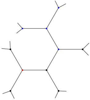
Figure 1. Illustration of the sets in formula (1.19) relative to the root $x_{\circ}$: $\varLambda=\{v\}$, $\partial\varLambda=\{x_{1},x_{2},\check{x}\}$ (here $\check{x}_{\mbox{$\;\!\!$}\varLambda}=v$), $\bar{\varLambda}=\{v,x_{1},x_{2},\check{x}\}$, and $\partial\varLambda^{\downarrow}=\{x_{1},x_{2}\}$ (see (1.18)).

1.2.5. Layout

The rest of the paper is organized as follows (cf. the table of contents). We state our main results in Section 2, starting with a general compatibility criterion (Theorem 2.1), which reduces the existence of SGM $\mu^{h}$ to the solvability of an infinite system of non-linear equations for permissible GBC $\{\boldsymbol{h}(x)\}$. This is followed by various sufficient conditions for uniqueness of SGM with uniform ferromagnetic interaction (Theorems 2.2, 2.3 and 2.5). As part of our general treatment of the Potts model on the Cayley tree, in Section 2.3.1 we introduce the notion of translation-invariant SGMs (based on a bijection between $\mathbb{T}^{k}$ and a free group with $k+1$ generators of period $2$ each), and state a novel criterion of translation invariance (Proposition 2.6) in terms of the external field and the GBC.

Non-uniqueness results for a subclass of completely homogeneous SGMs (i.e., where the reduced fields $\{\check{\boldsymbol{\xi}}(x)\}$ and $\{\check{\boldsymbol{h}}(x)\}$ are constant) are summarized in Theorems 2.8, 2.9 and 2.10. The number of such measures is estimated in several special cases by $2^{q}-1$ (Theorem 2.11), and we conjecture that this is a universal upper bound. In Section 3, we record some auxiliary lemmas. The proofs of the uniqueness results (Theorems 2.2, 2.3 and 2.5) are presented in Section 4. Section 5 is devoted to the in-depth analysis of completely homogeneous SGMs, culminating in the proof of Theorems 2.8–2.11 (given in Sections 5.2–5.5, respectively). In Section 6, we study some fine properties (such as monotonicity, bounds and zeros) of the critical curves on the temperature–field plane, summarized in Propositions 6.4, 6.5, 6.11–6.14, 6.16 and 6.17. Finally, Appendix A presents the proof of Proposition 2.6, while Appendix B is devoted to the proof of a technical Lemma 5.3 addressing the special case $q=3$.

2. Results

2.1. Compatibility criterion

In view of Remark 1.2, when working with vectors and vector-valued functions and fields it will often be convenient to pass from a generic vector $\boldsymbol{u}=(u_{1},\dots,u_{q})\in\mathbb{R}^{q}$ to a “reduced vector” $\boldsymbol{\check{u}}=(\check{u}_{1},\dots,\check{u}_{q-1})\in\mathbb{R}^{q-1}$ by setting $\check{u}_{i}:=u_{i}-u_{q}$ ($i=1,\dots,q-1$).

The following general statement describes a criterion for the GBC $\{\boldsymbol{h}(x)\}_{x\in V}$ to guarantee compatibility of the measures $\{\mu^{h}_{n}\}_{n\in\mathbb{N}_{0}}$.

Theorem 2.1.

The probability distributions $\{\mu^{h}_{n}\}_{n\in\mathbb{N}_{0}}$ defined in (1.6) are compatible (and the underlying GBC $\{\boldsymbol{h}(x)\}_{x\in V}$ are permissible) if and only if the following vector identity holds

$$\beta\mbox{$\>\!$}\boldsymbol{\check{h}}(x)=\sum_{y\in S(x)}\boldsymbol{F}\bigl{(}\beta\mbox{$\>\!$}\boldsymbol{\check{h}}(y)+\beta\mbox{$\>\!$}\boldsymbol{\check{\xi}}(y);\mbox{$\>\!$}\mathrm{e}^{\beta J_{xy}}\bigr{)},\qquad x\in V,$$ (2.1)

where $\boldsymbol{\check{h}}(x)=(\check{h}_{i}(x),\dots,\check{h}_{q-1}(x))$,  $\boldsymbol{\check{\xi}}(x)=(\check{\xi}_{i}(x),\dots,\check{\xi}_{q-1}(x))$,

$$\check{h}_{i}(x):=h_{i}(x)-h_{q}(x),\qquad\check{\xi}_{i}(x):=\xi_{i}(x)-\xi_{q}(x),\qquad i=1,\dots,q-1,$$ (2.2)

and the map $\boldsymbol{F}(\boldsymbol{u};\theta)=(F_{1}(\boldsymbol{u};\theta),\dots,F_{q-1}(\boldsymbol{u};\theta))$ is defined for $\boldsymbol{u}=(u_{1},\dots,u_{q-1})\in\mathbb{R}^{q-1}$ and $\theta>0$ by the formulas

$$F_{i}(\boldsymbol{u};\theta):=\ln\frac{(\theta-1)\mbox{$\;\!$}\mathrm{e}^{u_{i}}+1+\sum_{j=1}^{q-1}\mathrm{e}^{u_{j}}}{\theta+\sum_{j=1}^{q-1}\mathrm{e}^{u_{j}}},\qquad i=1,\dots,q-1.$$ (2.3)

Remark 2.1.

Likewise, Theorem 2.1 is true for any of the $q$ possible reductions (see Remark 1.2).

Remark 2.2.

Note that $\boldsymbol{F}(\boldsymbol{0};\theta)=\boldsymbol{0}$ for any $\theta>0$.

Remark 2.3.

In view of the link (discussed in Section 1.2.4) between GBC $\{\boldsymbol{h}(x)\}_{x\in V}$ and boundary laws $\{\boldsymbol{z}(x,y)\}_{\langle x,y\rangle\in E}$, the compatibility criterion (2.1) is but a reformulation of the consistency property (1.13) of the boundary law.

By virtue of Theorem 2.1, if the GBC $\{\boldsymbol{h}(x)\}$ and the external field $\{\boldsymbol{\xi}(x)\}$ satisfy the functional equation (2.1) for some $\beta>0$ then there is a (unique) SGM $\mu^{h}_{\beta,\mbox{$\>\!$}\xi}$.

2.2. Uniqueness results

From now on, we confine ourselves to the case of uniform (ferromagnetic) nearest-neighbour interaction by setting $J_{xy}=J\geq 0$ if $d(x,y)=1$ (and $J_{xy}=0$ otherwise). It will also be convenient to re-parameterize the model by introducing the new parameter $\theta=\mathrm{e}^{\beta J}\geq 1$ termed activity.

For $\theta\geq 1$, consider the function

$$\varphi(t;\theta):=\frac{(\theta-1)\mbox{$\;\!$}t}{\bigl{(}\sqrt{\theta\mbox{$\>\!$}(t-1)}+\sqrt{t-\theta}\mbox{$\;\!$}\bigr{)}^{2}},\qquad t\geq\theta,$$ (2.4)

which can also be written as

$$\varphi(t;\theta)=\frac{\sqrt{\theta\mbox{$\>\!$}(t-1)}-\sqrt{t-\theta}}{\sqrt{\theta\mbox{$\>\!$}(t-1)}+\sqrt{t-\theta}},\qquad t\geq\theta.$$ (2.5)

Noting that

$$\varphi(t;\theta)=\frac{\theta-1}{\left(\sqrt{\theta-\theta/t}+\sqrt{1-\theta/t}\mbox{$\;\!$}\right)^{2}},$$

it is evident that $t\mapsto\varphi(t;\theta)$ is a decreasing function; in particular, for all $t\geq\theta$

$$1=\varphi(\theta;\theta)\geq\varphi(t;\theta)\geq\varphi(\infty;\theta)=\frac{\sqrt{\theta}-1}{\sqrt{\theta}+1}.$$ (2.6)

For brevity, introduce the notation

$$Q(\theta):=(q-2)\mbox{$\;\!$}\frac{\sqrt{\theta}-1}{\sqrt{\theta}+1},$$ (2.7)

and for $k\geq 2$, $q\geq 2$ consider the equation

$$Q(\theta)+\varphi(\theta+1;\theta)=\frac{1}{k},\qquad\theta\geq 1,$$ (2.8)

or more explicitly (noting that $\varphi(\theta+1;\theta)=(\theta-1)/(\theta+1)$),

$$Q(\theta)+\frac{\theta-1}{\theta+1}=\frac{1}{k},\qquad\theta\geq 1.$$ (2.9)

The left-hand side of (2.9) is a continuous increasing function of $\theta\in[1,\infty)$ ranging from $0$ to $q-1>k^{-1}$, which implies that there is a unique solution of the equation (2.9), denoted $\theta_{0}=\theta_{0}(k,q)$. In particular, for $q=2$ we get

$$\theta_{0}(k,2)=\frac{k+1}{k-1}.$$ (2.10)

Let us also consider the equation

$$(q-1)\mbox{$\;\!$}\frac{\theta-1}{\theta+1}=\frac{1}{k},$$ (2.11)

which has the unique root

$$\theta_{*}=\theta_{*}(k,q):=\frac{k(q-1)+1}{k(q-1)-1}.$$ (2.12)

Noting from (2.7) that, for any $\theta>1$,

$$(q-1)\mbox{$\;\!$}\frac{\sqrt{\theta}-1}{\sqrt{\theta}+1}<Q(\theta)+\frac{\theta-1}{\theta+1}\leq(q-1)\mbox{$\;\!$}\frac{\theta-1}{\theta+1},$$

and comparing equations (2.9) and (2.11), it follows that

$$\theta_{*}(k,q)\leq\theta_{0}(k,q)<\left(\theta_{*}(k,q)\right)^{2},$$

where the first inequality is in fact strict unless $q=2$.

Theorem 2.2.

Let $\theta_{0}=\theta_{0}(k,q)$ be the unique solution of the equation (2.9). Then the Gibbs measure $\mu_{\theta,\mbox{$\>\!$}\xi}$ is unique for $\theta\in(1,\theta_{0})$ and any external field $\boldsymbol{\xi}$.

Remark 2.4.

It is known that the Ising model on a Cayley tree with zero external field has a unique Gibbs measure if and only if $\theta\leq\theta_{\rm c}(k)=\sqrt{1+\vphantom{(^{T}}\smash{\frac{2}{k-1}}}$  (see [8]); that is to say, $\theta_{\rm c}(k)$ is the critical activity of the Ising model. Since $\theta_{\rm c}(k)=\theta_{0}(k,2)$, our Theorem 2.2 is sharp in this case. Let $\theta_{\rm cr}(k,q)$ be the critical activity for the Potts model; its exact value is known only for the binary tree ($k=2$), namely $\theta_{\rm cr}(2,q)=1+2\sqrt{q-1}\,$ [30]. Note that $\theta_{\rm cr}(2,2)=\theta_{0}(2,2)\,(=3)$ but $\theta_{\rm cr}(2,q)>\theta_{0}(2,q)$ for $q\geq 3$, so Theorem 2.2 is not sharp already for $k=2$, $q\geq 3$.

For $k\geq 2$, $q\geq 2$ and any $\gamma\in\mathbb{R}$, consider the equation (cf. (2.8))

$$Q(\theta)+\varphi\bigl{(}t_{\gamma}(\theta);\theta\bigr{)}=\frac{1}{k},\qquad\theta\geq 1,$$ (2.13)

where $\varphi(t;\theta)$ and $Q(\theta)$ are defined in (2.4) and (2.7), respectively, and

$$t_{\gamma}(\theta):=\theta+1+(q-2)\mbox{$\;\!$}\theta^{\gamma}.$$ (2.14)

It can be shown (see Lemma 3.5) that equation (2.13) has a unique root, $\theta^{*}_{\mbox{$\;\!\!$}\gamma}=\theta^{*}_{\mbox{$\;\!\!$}\gamma}(k,q)$. More specifically, if $q=2$ then $t_{\gamma}(\theta)=\theta+1$ and equation (2.13) is reduced to equation (2.8) (with $Q(\theta)\equiv 0$), so that $\theta_{\gamma}^{*}(k,2)\equiv\theta_{0}(k,2)=(k+1)/(k-1)$ (see (2.10)). However, if $q\geq 3$ then the root $\theta^{*}_{\mbox{$\;\!\!$}\gamma}$ is an increasing function of parameter $\gamma$ with the asymptotic bounds

$$\theta_{0}(k,q)=\lim_{\gamma\to-\infty}\theta^{*}_{\mbox{$\;\!\!$}\gamma}(k,q)<\theta^{*}_{\mbox{$\;\!\!$}\gamma}(k,q)<\lim_{\gamma\to+\infty}\theta^{*}_{\mbox{$\;\!\!$}\gamma}(k,q)=\left(\theta_{*}(k,q)\right)^{2}.$$ (2.15)

Definition 2.1.

Given the external field $\boldsymbol{\xi}(x)=(\xi_{1}(x),\dots,\xi_{q}(x))$ ($x\in V$), define the asymptotic “gap” between its coordinates as follows,

$$\varDelta^{\xi}:=\max_{1\leq\ell\leq q}\liminf_{x\in V}\,{}_{\ell}\check{\xi}_{(1)}(x),$$ (2.16)

where

$${}_{\ell}\check{\xi}_{(1)}(x):=\min_{i\neq\ell}{}_{\ell}\check{\xi}_{i}(x)\equiv\min_{i\neq\ell}(\xi_{i}(x)-\xi_{\ell}(x)),\qquad x\in V.$$ (2.17)

Theorem 2.3.

The Gibbs measure $\mu_{\beta,\mbox{$\>\!$}\xi}$ is unique for any $\beta\in\bigl{(}0,\ln\theta^{*}_{\mbox{$\>\!\!$}\varDelta^{\xi}-k}\bigr{)}$, where $\theta_{\gamma}^{*}\!$ denotes the unique solution of the equation (2.13).

Remark 2.5.

As already mentioned, if $q=2$ then $\theta_{\gamma}^{*}(k,2)\equiv\theta_{0}(k,2)$ and we recover Theorem 2.2 in this case. But if $q\geq 3$ then $\theta_{\mbox{$\>\!\!$}\mbox{$\>\!$}\gamma}^{*}(k,q)>\theta_{0}(k,q)$ for any $\gamma\in\mathbb{R}$ (see (2.15)), so that Theorem 2.3 ensures the uniqueness of the SGM $\mu_{\beta,\mbox{$\>\!$}\xi}$ on a wider interval of temperatures as compared to Theorem 2.2, for any $\varDelta^{\xi}$. Moreover, due to the monotonicity of the map $\gamma\mapsto\theta_{\mbox{$\>\!\!$}\mbox{$\>\!$}\gamma}^{*}$ (Lemma 3.5), a larger gap $\varDelta^{\xi}$ facilitates uniqueness of SGM; however, the domain of guaranteed uniqueness (in parameter $\theta$) is bounded in all cases (see (2.15)) by $(\theta_{*}(k,q))^{2}\leq(\theta_{*}(2,3))^{2}=25/9\doteq 2.7778$.

Remark 2.6.

If the external field $\boldsymbol{\xi}$ is random then the gap (2.16) is a random variable measurable with respect to the “tail” $\sigma$-algebra $\mathscr{F}^{\infty}=\bigcap_{n=0}^{\infty}\sigma\{\boldsymbol{\xi}(x),\,x\in V_{n}^{c}\}$. Intuitively, this means that $\varDelta^{\xi}$ does not depend on the values of the field $\boldsymbol{\xi}(x)$ on any finite set $\varLambda\subset V$. If the values of $\boldsymbol{\xi}(x)$ are assumed to be independent (not necessarily identically distributed) for different $x\in V$ then, by Kolmogorov’s zero–one law, $\varDelta^{\xi}=\mathrm{const}$ (and therefore $\theta^{*}_{\mbox{$\>\!\!$}\varDelta^{\xi}-k}=\mathrm{const}$) almost surely (a.s.).

Example 2.1.

Let us compute the asymptotic gap $\varDelta^{\xi}$ in a few examples.

• Let the random vectors $\boldsymbol{\xi}(x)$ ($x\in V$) be mutually independent, with independent and identically distributed (i.i.d.) coordinates $\xi_{i}(x)$ ($i=1,\dots,q)$, each taking the values $\pm 1$ with probabilities $\frac{1}{2}$. Note that ${}_{\ell}\check{\xi}_{(1)}(x)\in\{0,\pm 2\}$  ($\ell=1,\dots,q$) and

  $$\mathbb{P}\bigl{(}{}_{\ell}\check{\xi}_{(1)}(x)=-2\bigr{)} =\mathbb{P}\Bigl{(}\xi_{\ell}(x)=1,\,\min_{i\neq\ell}\xi_{i}(x)=-1\Bigr{)}$$

  $$=\mathbb{P}\bigl{(}\xi_{\ell}(x)=1\bigr{)}\cdot\bigl{(}1-\mathbb{P}(\xi_{i}(x)=1,\,i\neq\ell)\bigr{)}$$

  $$=\tfrac{1}{2}\Bigl{(}1-\left(\tfrac{1}{2}\right)^{q-1}\Bigr{)}>0.$$ (2.18)

  The Borel–Cantelli lemma then implies that $\liminf_{x\in V}{}_{\ell}\check{\xi}_{(1)}(x)=-2$ a.s. and hence, according to (2.16), $\varDelta^{\xi}=-2$ a.s.

• In the previous example, let us remove the i.i.d. assumption for the coordinates, and instead suppose that each of the random vectors $\boldsymbol{\xi}(x)$ (still mutually independent for different $x\in V$) can take two values, $\pm(1,\dots,1)$, with probability $\frac{1}{2}$ each. Then it is clear that ${}_{\ell}\check{\xi}_{(1)}(x)\equiv 0$ ($\ell=1,\dots,q$), hence $\varDelta^{\xi}=0$ a.s.

• Extending example (b), suppose that, with some $\alpha\in\mathbb{R}$,

  $$\mathbb{P}\bigl{(}\xi_{i}(x)=\alpha\ \text{and}\ \xi_{j}(x)=0\ \text{for all}\ j\neq i\bigr{)}=q^{-1}\qquad(i=1,\dots,q).$$

  Of course, for $\alpha=0$ we have $\boldsymbol{\xi}(x)\equiv\boldsymbol{0}$ and hence $\varDelta^{\xi}=0$; thus, let $\alpha\neq 0$. If $q=2$ then it is straightforward to see that

  $$\mathbb{P}\bigl{(}{}_{\ell}\check{\xi}_{(1)}(x)=\pm\alpha\bigr{)}=\tfrac{1}{2},\qquad\ell=1,2.$$

  For $q\geq 3$, if $\alpha>0$ then, similarly,

  $$\mathbb{P}\bigl{(}{}_{\ell}\check{\xi}_{(1)}(x)=-\alpha\bigr{)}=q^{-1},\qquad\mathbb{P}\bigl{(}{}_{\ell}\check{\xi}_{(1)}(x)=0\bigr{)}=1-q^{-1},$$ (2.19)

  whereas if $\alpha<0$ then

  $$\mathbb{P}\bigl{(}{}_{\ell}\check{\xi}_{(1)}(x)=-\alpha\bigr{)}=q^{-1},\qquad\mathbb{P}\bigl{(}{}_{\ell}\check{\xi}_{(1)}(x)=\alpha\bigr{)}=1-q^{-1}.$$ (2.20)

  Thus, in all cases, the Borel–Cantelli lemma yields that $\varDelta^{\xi}=-|\alpha|$ a.s. (which also includes the case $\alpha=0$).

• Consider i.i.d. vectors $\boldsymbol{\xi}(x)$ ($x\in V$) with i.i.d. coordinates $\xi_{i}(x)$ ($i=1,\dots,q)$, each with the uniform distribution on $[0,1]$. Note that $-1\leq{}_{\ell}\check{\xi}_{(1)}(x)\leq 1$ ($\ell=1,\dots,q$) and, for any $\varepsilon\in(0,1)$,

  $$\mathbb{P}\bigl{(}{}_{\ell}\check{\xi}_{(1)}(x)\leq-1+2\varepsilon\bigr{)} \geq\mathbb{P}\Bigl{(}\xi_{\ell}(x)\geq 1-\varepsilon,\,\min_{i\neq\ell}\xi_{i}(x)\leq\varepsilon\Bigr{)}$$

  $$=\mathbb{P}\bigl{(}\xi_{\ell}(x)\geq 1-\varepsilon\bigr{)}\cdot\Bigl{(}1-\mathbb{P}\bigl{\{}\min_{i\neq\ell}\xi_{i}(x)\geq\varepsilon\bigr{\}}\Bigr{)}$$

  $$=\varepsilon\left(1-(1-\varepsilon)^{q-1}\right)>0.$$

  The Borel–Cantelli lemma then implies that $\liminf_{x\in V}{}_{\ell}\check{\xi}_{(1)}(x)\leq-1+2\varepsilon$ a.s., and since $\varepsilon>0$ is arbitrary, it follows that $\liminf_{x\in V}{}_{\ell}\check{\xi}_{(1)}(x)=-1$ a.s., for each $\ell=1,\dots,q$; hence, according to (2.16), $\varDelta^{\xi}=-1$ a.s.

• For a “non-ergodic” type of example leading to a random gap $\varDelta^{\xi}$, suppose that $\boldsymbol{\xi}(x)\equiv\boldsymbol{\xi}(x_{\circ})$ ($x\in V$), where the distribution of $\boldsymbol{\xi}(x_{\circ})$ is as in example (a). That is to say, the values of the field $\boldsymbol{\xi}(x)$ are obtained by duplicating its (random) value at the root. Then, similarly to (2.18), we compute

  $$\mathbb{P}(\varDelta^{\xi}=-2)=\tfrac{1}{2}-\left(\tfrac{1}{2}\right)^{q},\qquad\mathbb{P}(\varDelta^{\xi}=2)=\left(\tfrac{1}{2}\right)^{q},\qquad\mathbb{P}(\varDelta^{\xi}=0)=\tfrac{1}{2}.$$

• Finally, the simplest “coordinate-oriented” choice $\boldsymbol{\xi}(x)\equiv(\alpha,0,\dots,0)$, $x\in V$, with a fixed $\alpha\in\mathbb{R}$, exemplifies translation-invariant (non-random) external fields, including the case of zero field, $\alpha=0$. Our results for this model will be stated in Section 2.3; for now, let us calculate the value of the gap $\varDelta^{\xi}$. Again, for $\alpha=0$ we have $\boldsymbol{\xi}(x)\equiv\boldsymbol{0}$ and hence $\varDelta^{\xi}=0$; thus, let $\alpha\neq 0$. If $q=2$ then ${}_{1}\check{\xi}_{(1)}(x)=-\alpha$, ${}_{2}\check{\xi}_{(1)}(x)=\alpha$, hence it is easy to see that $\varDelta^{\xi}=\max\{-\alpha,\alpha\}=|\alpha|$. For $q\geq 3$, if $\alpha>0$ then ${}_{1}\check{\xi}_{(1)}(x)=-\alpha$ and ${}_{\ell}\check{\xi}_{(1)}(x)=0$ ($\ell\neq 1$), whereas if $\alpha<0$ then still ${}_{1}\check{\xi}_{(1)}(x)=-\alpha$ but ${}_{\ell}\check{\xi}_{(1)}(x)=\alpha$ ($\ell\neq 1$); as a result, $\varDelta^{\xi}=0$ for $\alpha\geq 0$ and $\varDelta^{\xi}=|\alpha|$ for $\alpha<0$.

The following general assertion summarizes Example 2.1. Recall that random variables $X_{1},\dots,X_{q}$ are said to be exchangeable if the distribution of the random vector $(X_{1},\dots,X_{q})$ is invariant with respect to permutations of the coordinates. The support $\operatorname{\rm supp}X$ of (the distribution of) a random variable $X$ is defined as the (closed) set comprising all points $u\in\mathbb{R}$ such that for any $\varepsilon>0$ we have $\mathbb{P}(|X-u|\leq\varepsilon)>0$.

Proposition 2.4.

Suppose that the random vectors $\{\boldsymbol{\xi}(x)\}_{x\in V}$ are i.i.d., and for each $x\in V$ their coordinates $\xi_{1}(x),\dots,\xi_{q}(x)$ are exchangeable. Then

$$\varDelta^{\xi}=\inf\{\operatorname{\rm supp}\left(\xi_{1}(x)-\xi_{q}(x)\right)\}\quad\text{a.s.}$$

In particular, $\varDelta^{\xi}<0$ a.s., unless $\xi_{1}(x)=\dots=\xi_{q}(x)$ a.s., in which case $\varDelta^{\xi}=0$ a.s.

Proof.

Observe that, by exchangeability of $\{\xi_{i}(x)\}$, the distribution of ${}_{\ell}\xi_{(1)}(x)$ does not depend on $\ell=1,\dots,q$ and, moreover,

$$\operatorname{\rm supp}{}_{\ell}\check{\xi}_{(1)}(x)=\operatorname{\rm supp}\left(\xi_{1}(x)-\xi_{q}(x)\right).$$ (2.21)

Denote $u_{0}:=\inf\{\operatorname{\rm supp}\left(\xi_{1}(x)-\xi_{q}(x)\right)\}$. From (2.21), it follows that ${}_{\ell}\check{\xi}_{(1)}(x)\geq u_{0}$ a.s., and therefore, according to (2.16), $\varDelta^{\xi}\geq u_{0}$ a.s. On the other hand, for any $\varepsilon>0$ we have

$$\mathbb{P}\bigl{(}{}_{\ell}\check{\xi}_{(1)}(x)\leq u_{0}+\varepsilon\bigr{)}=\mathbb{P}\bigl{(}\xi_{1}(x)-\xi_{q}(x)\leq u_{0}+\varepsilon\bigr{)}>0,$$

and the Borel–Cantelli lemma implies that $\liminf_{x\in V}{}_{\ell}\check{\xi}_{(1)}(x)\leq u_{0}+\varepsilon$ a.s., so that $\varDelta^{\xi}\leq u_{0}$ a.s. As a result, $\varDelta^{\xi}=u_{0}$ a.s., as claimed. ∎

Theorem 2.5.

Assume that the random external field $\boldsymbol{\xi}=\{\boldsymbol{\xi}(x)\}_{x\in V}$ is as in Proposition 2.4. Let $\theta^{{\dagger}}=\theta^{{\dagger}}(k,q)$ be the root of the equation

$$Q(\theta)+\mathbb{E}\bigl{\{}\varphi\bigl{(}t_{\check{\xi}_{(1)}(x)-k}(\theta);\theta\bigr{)}\bigr{\}}=\frac{1}{k},\qquad\theta\geq 1,$$ (2.22)

where $\check{\xi}_{(1)}(x)\equiv{}_{q}\mbox{$\>\!$}\check{\xi}_{(1)}(x)=\min_{i\neq q}\bigl{(}\xi_{i}(x)-\xi_{q}(x)\bigr{)}$ (cf. (2.17)) and the notation $t_{\gamma}(\theta)$ is introduced in (2.14). Then, for each $\theta\in[1,\theta^{{\dagger}})$ and for $\mathbb{P}$-almost all realizations of the random field $\boldsymbol{\xi}$, there is a unique Gibbs measure $\mu_{\theta,\mbox{$\>\!$}\xi}$.

Remark 2.7.

Note that Theorem 2.3 guarantees uniqueness of the Gibbs measure in the interval $1<\theta<\theta^{*}_{\mbox{$\>\!\!$}\varDelta^{\xi}-k}$, where $\theta^{*}_{\mbox{$\>\!\!$}\varDelta^{\xi}-k}$ is the solution of the equation

$$Q(\theta)+\varphi\bigl{(}t_{\mbox{$\;\!\!$}\varDelta^{\xi}-k}(\theta);\theta\bigr{)}=\frac{1}{k},\qquad\theta\geq 1.$$

By Proposition 2.4, we have $\check{\xi}_{(1)}(x)\geq\varDelta^{\xi}$ (a.s.), and moreover, $\check{\xi}_{(1)}(x)>\varDelta^{\xi}$ with positive probability, unless $\xi_{1}(x)=\dots=\xi_{q}(x)$ a.s. Thus, excluding the case $q=2$ where $t_{\gamma}(\theta)=\theta+1$, by monotonicity of the function $\gamma\mapsto\varphi(t_{\gamma};\theta)$ we conclude that $\theta^{*}_{\mbox{$\>\!\!$}\varDelta^{\xi}-k}(k,q)<\theta^{{\dagger}}(k,q)$, and therefore the domain of uniqueness in Theorem 2.5 is wider than that in Theorem 2.3.

Example 2.2.

Let us illustrate Theorem 2.5 with a simple model described in Example 2.1(c), assuming that $q\geq 3$. Suppose first that $\alpha>0$. Then, according to the distribution (2.19) and notation (2.14), equation (2.22) specializes to

$$Q(\theta)+\frac{1}{q}\,\varphi\left(\theta+1+\frac{q-2}{\theta^{\alpha+k}_{\vphantom{X}}};\theta\right)+\frac{q-1}{q}\,\varphi\left(\theta+1+\frac{q-2}{\theta^{k}};\theta\right)=\frac{1}{k}.$$

By monotonicity of the function $t\mapsto\varphi(t;\theta)$, it is clear that the root $\theta^{{\dagger}}$ of this equation is strictly bigger than the root $\theta^{*}_{\mbox{$\>\!\!$}\varDelta^{\xi}-k}=\theta^{*}_{-\alpha-k}$ of the equation

$$Q(\theta)+\varphi\left(\theta+1+\frac{q-2}{\theta^{\alpha+k}_{\vphantom{X}}};\theta\right)=\frac{1}{k},$$

in accordance with Remark 2.7. Similarly, if $\alpha<0$ then the distribution (2.19) is replaced by (2.20) and equation (2.22) takes the form

$$Q(\theta)+\frac{1}{q}\,\varphi\left(\theta+1+\frac{q-2}{\theta^{\alpha+k}_{\vphantom{X}}};\theta\right)+\frac{q-1}{q}\,\varphi\left(\theta+1+\frac{q-2}{\theta^{-\alpha+k}_{\vphantom{X}}};\theta\right)=\frac{1}{k},$$

and by the monotonicity argument it is evident that its root $\theta^{{\dagger}}$ is strictly bigger than the root $\theta^{*}_{\mbox{$\>\!\!$}\varDelta^{\xi}-k}=\theta^{*}_{\alpha-k}$ of the equation

$$Q(\theta)+\varphi\left(\theta+1+\frac{q-2}{\theta^{-\alpha+k}};\theta\right)=\frac{1}{k},$$

again confirming the observation of Remark 2.7.

2.3. Translation-invariant SGM and the problem of non-uniqueness

2.3.1. Translation invariance

To introduce the notion of translations on the Cayley tree $\mathbb{T}^{k}$ , let $\mathscr{A}_{k}$ be the free group with generators $a_{1},\dots,\allowbreak a_{k+1}$ of order $2$ each (i.e., $a_{i}^{-1}=a_{i}$). It is easy to see (cf. [20] and also [47, Section 2.2]) that the Cayley tree $\mathbb{T}^{k}=(V,E)$ is in a one-to-one correspondence with the group $\mathscr{A}_{k}$. Namely, start by associating the root $x_{\circ}\in V$ with the identity element $e\in\mathscr{A}_{k}$, and identify the elements $a_{1},\dots,a_{k+1}$ with the $k+1$ nearest neighbours of $x_{\circ}$ (i.e., comprising the set $S(x_{\circ})=W_{1}$). Proceed inductively by expanding the elements $a\in\mathscr{A}_{k}$ along the tree via right-multiplication by the generators $a_{i}$ $(i=1,\dots,k+1$), yielding $k$ new elements corresponding to the set of direct successors of $a$ (see Figure 2). This establishes a bijection $\mathfrak{b}\colon V\!\rightarrow\mathscr{A}_{k}$.

Consider the family of left shifts $T_{g}\colon\mathscr{A}_{k}\to\mathscr{A}_{k}$ ($g\in\mathscr{A}_{k}$) defined by

$$T_{g}(a):=g\mbox{$\>\!$}a,\qquad a\in\mathscr{A}_{k}.$$

By virtue of the bijection $\mathfrak{b}$, this determines conjugate translations on $V$,

$$\widetilde{T}_{z}:=\mathfrak{b}^{-1}\mbox{$\>\!\!$}\circ T_{\mathfrak{b}(z)}\mbox{$\;\!\!$}\circ\mathfrak{b},\qquad z\in V.$$ (2.23)

Clearly, $\widetilde{T}_{z}$ is an automorphism of $V$ preserving the nearest-neighbour relation; indeed, if $\langle x,y\rangle\in E$ and $y\in S(x)$ (so that $\mathfrak{b}(y)=\mathfrak{b}(x)\mbox{$\;\!$}a_{j}$, with some generator $a_{j}$) then, according to (2.23), $x^{\prime}\mbox{$\>\!\!$}:=\widetilde{T}_{z}(x)$ and $y^{\prime}\mbox{$\>\!\!$}:=\widetilde{T}_{z}(y)=\mathfrak{b}^{-1}(\mathfrak{b}(z)\mbox{$\>\!$}\mathfrak{b}(y))=\mathfrak{b}^{-1}(\mathfrak{b}(x^{\prime})\mbox{$\;\!$}a_{j})$ are nearest neighbours, $\langle x^{\prime}\mbox{$\;\!\!$},y^{\prime}\rangle\in E$ (see Figure 2). For example, if $k=1$ (whereby the Cayley tree $\mathbb{T}^{1}$ is reduced to the integer lattice $\mathbb{Z}^{1}$), the action of the shift $\widetilde{T}_{z}$ ($z\in\mathbb{Z}^{1}$) can be written in closed form,

$$\widetilde{T}_{z}(x)=z+(-1)^{z}x,\qquad x\in\mathbb{Z}^{1}.$$

In turn, the map (2.23) induces shifts on configurations $\sigma\in\varPhi^{V}$,

$$(\widetilde{T}_{z}\mbox{$\>\!$}\sigma)(x):=\sigma(\widetilde{T}^{-1}_{z}x),\qquad x\in V.$$ (2.24)

Definition 2.2.

We say that SGM $\mu^{h}=\mu^{h}_{\theta,\mbox{$\>\!$}\xi}$ is translation invariant (with respect to the group of shifts $(\widetilde{T}_{z})$) if for each $z\in V$ the measures $\mu^{h}\circ\widetilde{T}_{z}^{-1}$ and $\mu^{h}$ coincide; that is, for any (finite) $\varLambda\subset V$ and any configuration $\varsigma\in\varPhi^{\varLambda}$

$$\mu^{h}\bigl{(}\sigma_{\widetilde{T}_{z}(\varLambda)}=\widetilde{T}_{z}(\varsigma)\bigr{)}=\mu^{h}(\sigma_{\mbox{$\;\!\!$}\varLambda}=\varsigma).$$ (2.25)

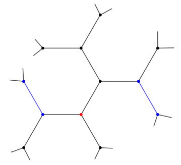
Figure 2. A fragment of the Cayley tree $\mathbb{T}^{2}$ $(k=2$), with vertices represented (one-to-one) by elements of the free group $\mathscr{A}_{2}$ with generators $\{a_{1},a_{2},a_{3}\}$ (of order $2$ each). The identity element $e\in\mathscr{A}_{2}$ designates the root $x_{\circ}\in V$. Starting from $e$, the elements $a\in\mathscr{A_{2}}$ are inductively expanded along the tree via right-multiplication by one of the generators. Translations on $\mathscr{A}_{2}$ are defined as left shifts, $T_{g}\colon a\to ga$ ($g,a\in\mathscr{A}_{2}$). For example, under the shift $T_{a_{1}}\!$ the edge $\langle a_{2},a_{2}\mbox{$\>\!$}a_{3}\rangle$ is mapped to the edge $\langle a_{1}a_{2},a_{1}a_{2}\mbox{$\>\!$}a_{3}\rangle$.

Recall that the quantities $\check{h}_{i}^{\dagger}(x,y)$ ($\langle x,y\rangle\in E$) defining the boundary law were introduced in Section 1.2.4.

Proposition 2.6.

An SGM $\mu^{h}=\mu^{h}_{\theta,\mbox{$\>\!$}\xi}$ is translation invariant under the group of shifts $(\widetilde{T}_{z})_{z\in V}$ if and only if the following conditions are satisfied.

• The reduced field $\{\check{\boldsymbol{\xi}}(x)\}$ is constant over the tree,

  $$\check{\boldsymbol{\xi}}(x)=\check{\boldsymbol{\xi}}(x_{\circ}),\qquad x\in V.$$ (2.26)

• The reduced field $\{\check{\boldsymbol{h}}{}^{\dagger}(x,y)\}$ is symmetric,

  $$\check{\boldsymbol{h}}{}^{\dagger}(x,y)=\check{\boldsymbol{h}}{}^{\dagger}(y,x),\qquad\langle x,y\rangle\in E.$$ (2.27)

• For any $z\in V$,

  $$\check{\boldsymbol{h}}{}^{\dagger}(x,y)=\check{\boldsymbol{h}}{}^{\dagger}\mbox{$\;\!\!$}\bigl{(}\widetilde{T}_{z}(x),\widetilde{T}_{z}(y)\bigr{)},\qquad\langle x,y\rangle\in E.$$ (2.28)

This result will be proved in Appendix A.

For $x\neq x_{\circ}$, denote by $x^{\prime}\mbox{$\>\!\!$}$ the unique vertex such that $x\in S(x^{\prime})$. Then, according to (1.17) and (2.28),

$$\check{\boldsymbol{h}}{}^{\dagger}(x,x^{\prime})=\check{\boldsymbol{h}}(x)=\check{\boldsymbol{h}}\bigl{(}\widetilde{T}^{-1}_{x^{\prime}}(x)\bigr{)}.$$ (2.29)

Note that $\widetilde{T}^{-1}_{x^{\prime}}(x)\in\partial\{x_{\circ}\}=W_{1}$. Thus, there are $k+1$ (vector) values $\check{\boldsymbol{h}}(x_{j})$ ($x_{j}\in W_{1}$) that determine a translation-invariant SGM $\mu^{h}$. By translations (2.29), these values (which can be pictured as $k+1$ “colours”) are propagated to all vertices $x\in V$ in a periodic “chessboard” tiling, except the root $x=x_{\circ}$ where the value $\check{\boldsymbol{h}}(x_{\circ})$ is calculated separately, according to the compatibility formula (2.1).

The criterion of translation invariance given by Proposition 2.6 appears to be new. In Georgii [22, Corollary (12.17)], a version of this result is established (in the language of boundary laws) for completely homogeneous SGM, that is, assuming the invariance under the group of all automorphisms of the tree $\mathbb{T}^{k}$. Namely, we have the following

Corollary 2.7.

An SGM $\mu^{h}=\mu^{h}_{\theta,\mbox{$\>\!$}\xi}$ is completely homogeneous if and only if  $\check{\boldsymbol{\xi}}(x)\equiv\check{\boldsymbol{\xi}}{}^{0}\mbox{$\>\!\!$}$ for all $x\in V$ and $\check{\boldsymbol{h}}(x)\equiv\check{\boldsymbol{h}}{}^{0}\mbox{$\>\!\!$}$ for all $x\neq x_{\circ}$.

Remark 2.8.

In the existing studies of Gibbs measures on trees (see, e.g., [19, 30]), it is common to use the term “translation invariant” (and the abbreviation TISGM) having in mind just completely homogeneous SGM. We prefer to keep the terminological distinction between “single-coloured” completely homogeneous GBC $\check{\boldsymbol{h}}(x)\equiv\check{\boldsymbol{h}}{}^{0}\mbox{$\>\!\!$}$ and “multi-coloured” translation-invariant GBC as characterized by Proposition 2.6. The latter case is very interesting (especially with regard to uniqueness) but technically more challenging, so it is not addressed here in full generality. However, as we will see below, the subclass of completely homogeneous SGM in the Potts model is very rich in its own right.

2.3.2. Analysis of uniqueness

For the rest of Section 2.3, we deal with completely homogeneous SGM $\mu^{h}=\mu^{h}_{\theta,\mbox{$\>\!$}\xi}$, that is, with the external field $\{\boldsymbol{\xi}(x)\}_{x\in V}$ and GBC $\{\boldsymbol{h}(x)\}_{x\in V}$ satisfying the homogeneity conditions of Corollary 2.7. For simplicity, we confine ourselves to the case where all coordinates of the (reduced) vector $\check{\boldsymbol{\xi}}{}^{0}\mbox{$\>\!\!$}$ are zero except one; due to permutational symmetry, we may assume, without loss of generality, that $\check{\xi}_{1}^{0}=\alpha\in\mathbb{R}$ and $\check{\xi}^{0}_{2}=\dots=\check{\xi}^{0}_{q-1}=0$,

$$\boldsymbol{\check{\xi}}{}^{0}\mbox{$\>\!\!$}=(\alpha,0,\dots,0)\in\mathbb{R}^{q-1}.$$ (2.30)

We also write

$$\boldsymbol{\check{h}}{}^{0}\mbox{$\>\!\!$}=(\check{h}_{1}^{0},\dots,\check{h}_{q-1}^{0})\in\mathbb{R}^{q-1}.$$

Then, denoting $z_{i}:=\theta^{\mbox{$\;\!$}\check{h}_{i}^{0}/k}$ ($i=1,\dots,q-1$), the compatibility equations (2.1) are equivalently rewritten in the form

$$\left\{\begin{aligned} z_{1}&=1+\frac{(\theta-1)(\theta^{\alpha}z_{1}^{k}-1)}{\theta+\theta^{\alpha}_{\vphantom{X}}z_{1}^{k}+\sum_{j=2}^{q-1}z_{j}^{k}},\\ z_{i}&=1+\frac{(\theta-1)(z_{i}^{k}-1)}{\theta+\theta^{\alpha}_{\vphantom{X}}z_{1}^{k}+\sum_{j=2}^{q-1}z_{j}^{k}},\qquad i=2,\dots,q-1.\end{aligned}\right.$$ (2.31)

Solvability of the system (2.31) can be analysed in some detail; in particular, we are able to characterize the uniqueness of its solution, which in turn gives a criterion of the uniqueness of completely homogeneous SGM in the Potts model.

The case $\theta=1$ is trivial, as the system (2.31) will then have the unique solution $z_{1}=\dots=z_{q-1}=1$. The case $\theta>1$ and $\alpha=0$ has been studied in [29]; these results can be reproduced directly by the methods developed in the present work similarly to a more general (and difficult) case $\alpha\neq 0$, and are also obtainable in the limit as $\alpha\to 0$ (see Lemma 5.1(b) and Remark 5.1).

Thus, let us focus on the new case $\alpha\neq 0$. By Lemma 5.1(c), the system (2.31) with $\theta>1$ is reduced either to a single equation

$$u=1+\frac{(\theta-1)(\theta^{\alpha}u^{k}-1)}{\theta+\theta^{\alpha}_{\vphantom{X}}u^{k}+q-2}$$ (2.32)

or to the system of equations (indexed by $m=1,\dots,q-2$)

$$\left\{\begin{aligned} u&=1+\frac{(\theta-1)(\theta^{\alpha}u^{k}-1)}{\theta+\theta^{\alpha}_{\vphantom{X}}u^{k}+mv^{k}+q-2-m},\\ 1&=\frac{(\theta-1)(1+v+\dots+v^{k-1})}{\theta+\theta^{\alpha}_{\vphantom{X}}u^{k}+mv^{k}+q-2-m},\end{aligned}\right.$$ (2.33)

subject to the condition

$$v\neq 1.$$ (2.34)

Let us first address the solvability of the equation (2.32). Denote

$$\theta_{\rm c}=\theta_{\rm c}(k,q):=\frac{1}{2}\,\Biggl{(}\sqrt{(q-2)^{2}+4\mbox{$\>\!$}(q-1)\left(\frac{k+1}{k-1}\right)^{2}}-(q-2)\Biggr{)}.$$ (2.35)

In particular, if $q=2$ then $\theta_{\rm c}(k,2)=\frac{k+1}{k-1}\equiv\theta_{0}(k,2)$ (cf. (2.10)). Let us also set

$$b=b(\theta):=\frac{\theta\mbox{$\>\!$}(\theta+q-2)}{q-1}.$$ (2.36)

Clearly, $b(1)=1$ and $b(\theta)>1$ for $\theta>1$. Furthermore, comparing (2.35) and (2.36) observe that $b(\theta_{\rm c})=\left(\frac{k+1}{k-1}\right)^{2}$ and $b(\theta)>\left(\frac{k+1}{k-1}\right)^{2}$ for $\theta>\theta_{\rm c}$. For $\theta\geq\theta_{\rm c}$, denote by $x_{\pm}=x_{\pm}(\theta)$ the roots of the quadratic equation

$$(b+x)(1+x)=k\mbox{$\>\!$}(b-1)\mbox{$\>\!$}x$$ (2.37)

with discriminant

$$D=D(\theta):=\bigl{(}k\mbox{$\>\!$}(b-1)-(b+1)\bigr{)}^{2}-4b=(b-1)(k-1)^{2}\left(b-\left(\frac{k+1}{k-1}\right)^{2}\right),$$ (2.38)

that is,

$$x_{\pm}=x_{\pm}(\theta):=\frac{(b-1)(k-1)-2\pm\sqrt{D}}{2}.$$ (2.39)

Furthermore, introduce the notation

$$a_{\pm}=a_{\pm}(\theta):=\frac{1}{x_{\pm}}\left(\frac{1+x_{\pm}}{b+x_{\pm}}\right)^{k},\qquad\theta\geq\theta_{\rm c}.$$ (2.40)

Of course, $a_{-}(\theta_{\rm c})=a_{+}(\theta_{\rm c})$, and one can also show that $a_{-}(\theta)<a_{+}(\theta)$ for all $\theta>\theta_{\rm c}$ (see the proof of Theorem 2.8 in Section 5.2). Finally, denote

$$\alpha_{\pm}=\alpha_{\pm}(\theta):=-(k+1)+\frac{1}{\ln\theta}\ln\frac{q-1}{a_{\mp}},\qquad\theta\geq\theta_{\rm c},$$ (2.41)

so that $\alpha_{-}(\theta_{\rm c})=\alpha_{+}(\theta_{\rm c})$ and $\alpha_{-}(\theta)<\alpha_{+}(\theta)$ for $\theta>\theta_{\rm c}$.

Theorem 2.8.

Let $\nu_{0}(\theta,\alpha)$ denote the number of solutions $u>0$ of the equation (2.32). Then

$$\nu_{0}(\theta,\alpha)=\begin{cases}1&\text{if}\ \,\theta\leq\theta_{\rm c}\ \,\text{or}\ \,\theta>\theta_{\rm c}\ \,\text{and}\ \,\alpha\notin[\alpha_{-},\alpha_{+}],\\ 2&\text{if}\ \,\theta>\theta_{\rm c}\ \,\text{and}\ \,\alpha\in\{\alpha_{-},\alpha_{+}\},\\ 3&\text{if}\ \,\theta>\theta_{\rm c}\ \,\text{and}\ \,\alpha\in(\alpha_{-},\alpha_{+}),\end{cases}$$

where $\theta_{\rm c}$ is given in (2.35) and $\alpha_{\pm}=\alpha_{\pm}(\theta)$ are defined by (2.41).

Let us now state our results on the solvability of the set of equations (2.33). For each $m\in\{1,\dots,q-2\}$, consider the functions

$$L_{m}(v;\theta):={} (\theta-1)\mbox{$\;\!$}\bigl{(}v^{k-1}+\dots+v\bigr{)}-mv^{k}-(q-1-m),$$ (2.42)

$$K_{m}(v;\theta):={} \frac{\bigl{(}v^{k-1}+\dots+v+1\bigr{)}^{k}L_{m}(v;\theta)}{\bigl{(}v^{k-1}+\dots+v+L_{m}(v;\theta)\bigr{)}^{k}}.$$ (2.43)

It can be checked (see Lemma 5.2) that for any $\theta>1$ there is a unique value $v_{m}=v_{m}(\theta)>0$ such that

$$L_{m}^{*}(\theta):=L_{m}(v_{m};\theta)=\max_{v>0}L_{m}(v;\theta),$$

and moreover, the function $\theta\mapsto L_{m}^{*}(\theta)$ is strictly increasing. Denote by $\theta_{m}$ the (unique) value of $\theta>1$ such that

$$L_{m}^{*}(\theta_{m})=0.$$ (2.44)

Thus, for any $\theta>\theta_{m}$ the range of the functions $v\mapsto L_{m}(v;\theta)$ and $v\mapsto K_{m}(v;\theta)$ includes positive values,

$$\mathscr{V}_{m}^{+}(\theta):=\{v>0\colon L_{m}(v;\theta)>0\}\equiv\{v>0\colon K_{m}(v;\theta)>0\}\neq\varnothing,$$ (2.45)

and, therefore, the function

$$\alpha_{m}(\theta):=\frac{1}{\ln\theta}\max_{v\in\mathscr{V}_{m}^{+}(\theta)}\ln K_{m}(v;\theta)=\frac{\ln K_{m}^{*}(\theta)}{\ln\theta},\qquad\theta>\theta_{m},$$ (2.46)

is well defined, where

$$K_{m}^{*}(\theta):=\max_{v\in\mathscr{V}_{m}^{+}(\theta)}K_{m}(v;\theta).$$

Example 2.3.

In the case $k=2$, from (2.42) and (2.44) we obtain explicitly

$$\theta_{m}=1+2\sqrt{m\mbox{$\>\!$}(q-m-1)},\qquad m=1,\dots,q-2.$$ (2.47)

In particular, $\theta_{1}=1$ for $q=2$, and $\theta_{1}\geq 3$ whenever $q\geq 3$. Comparing (2.35) and (2.47), we also find that $\theta_{\rm c}\leq\theta_{1}$ if and only if $q\geq 6$. For example, for $q=5$ we have $\theta_{1}=1+2\sqrt{3}\doteq 4.4641$, $\theta_{2}=5$, $\theta_{\rm c}=\frac{1}{2}\mbox{$\>\!$}(\sqrt{153}-3)\doteq 4.6847$, that is, $\theta_{1}<\theta_{\rm c}<\theta_{2}$, whereas for $q=6$ and $q=7$ we compute $\theta_{1}=\theta_{\rm c}=5$ and $\theta_{1}=1+2\sqrt{5}\doteq 5.4721>\theta_{\rm c}=\frac{1}{2}\mbox{$\>\!$}(\sqrt{241}-5)\doteq 5.2621$, respectively. Another simple case is $q=3$ (with $m=1$ and any $k\geq 2$); indeed, it is easy to see that the condition (2.44) is satisfied with $v_{1}^{*}=v_{1}(\theta_{1})=1$ (cf. Lemma 5.2(c)), whence we readily find $\theta_{1}=1+\frac{2}{k-1}$.

Theorem 2.9.

For each $m\in\{1,\dots,q-2\}$, let $\nu_{m}(\theta,\alpha)$ denote the number of positive solutions $(u,v)$ of the system (2.33). Then $\nu_{m}(\theta,\alpha)\geq 1$ if and only if $\theta>\theta_{m}$ and $\alpha\leq\alpha_{m}(\theta)$.

As will be shown in Proposition 6.16(b), $\alpha_{+}(\theta)$ has a unique zero given by $\theta^{+}_{0}=1+\frac{q}{k-1}$, whereas $\alpha_{-}(\theta)$ has a unique zero $\theta^{-}_{0}$, which coincides with the zero $\theta_{1}^{\mbox{$\>\!$}0}$ of $\alpha_{1}(\theta)$. It also holds that $\alpha_{1}(\theta)$ is a majorant of the family of functions $\{\alpha_{m}(\theta)\}$ (see Propositions 6.11 and 6.12).

2.3.3. Uniqueness of completely homogeneous SGM

In the case $q=3$, there appears to be an additional critical value (see Lemma 5.3)

$$\tilde{\theta}_{1}=\tilde{\theta}_{1}(k):=\frac{5-k+\sqrt{49k^{2}+62k+49}}{6\mbox{$\>\!$}(k-1)}.$$ (2.48)

For example,

$$\tilde{\theta}_{1}(k)=\begin{cases}\displaystyle\frac{1+\sqrt{41}}{2}\doteq 3.7016,&k=2,\\[6.0pt] \displaystyle\ \frac{7}{3}\doteq 2.3333,&k=3,\\[6.0pt] \displaystyle\frac{1+\sqrt{1081}}{18}\doteq 1.8821,\ \ &k=4.\end{cases}$$ (2.49)

For $q\geq 2$, consider the following subsets of the half-plane $\{\theta\geq 1\}=\{(\theta,\alpha)\colon\theta\geq 1,\,\alpha\in\mathbb{R}\}$,

$$A_{q}:={} \{\theta>\theta_{\rm c},\,\alpha_{-}(\theta)\leq\alpha\leq\alpha_{+}(\theta)\},$$

$$B_{q}:={} \left\{\begin{aligned} &\,\varnothing&&\text{if\ \,}q=2,\\ &\{\theta>\theta_{1},\,\alpha<\alpha_{1}(\theta)\}\cup\{\theta>\tilde{\theta}_{1},\,\alpha=\alpha_{1}(\theta)\}\quad&&\text{if\ \,}q=3,\\ &\{\theta>\theta_{1},\,\alpha\leq\alpha_{1}(\theta)\}\quad&&\text{if\ \,}q\geq 4.\end{aligned}\right.$$ (2.50)

Denote the total number of positive solutions $\boldsymbol{z}=(z_{1},\dots,z_{q-1})$ of the system of equations (2.31) by $\nu(\theta,\alpha)$ ($\theta\geq 1$, $\alpha\in\mathbb{R}$); of course, this number also depends on $k$ and $q$. Theorems 2.8 and 2.9 can now be summarized as follows.

Theorem 2.10 (Non-uniqueness).

• If $q=2$ then $\nu(\theta,\alpha)\geq 2$ if and only if $(\theta,\alpha)\in A_{2}\cup B_{2}=A_{2}$.

• If $q=3$ then $\nu(\theta,\alpha)\geq 2$ if $(\theta,\alpha)\in A_{3}\cup B_{3}$. The “only if” statement holds true at least for $k=2,3,4$.

• If $q\geq 4$ then $\nu(\theta,\alpha)\geq 2$ if and only if $(\theta,\alpha)\in A_{q}\cup B_{q}$.

Remark 2.9.

The special case $q=3$ in the definition (2.50) and in Theorem 2.10 emerges because for $\theta\leq\tilde{\theta}_{1}$ and $\alpha=\alpha_{1}(\theta)$, there is a (hypothetically unique) solution $(u,v)=\bigl{(}\theta-\frac{\theta+2}{k},1\bigr{)}$ of the system (2.33), which is, however, not admissible due to the constraint (2.34) and, therefore, does not destroy the uniqueness of solution to (2.31). This hypothesis is conjectured below; if it is true then “if” in Theorem 2.10(b) (i.e., $q=3$) can be enhanced to “if and only if” for all $k\geq 2$.

Conjecture 2.1.

If $q=3$, $\theta\leq\tilde{\theta}_{1}$ and $\alpha=\alpha_{1}(\theta)$ then $(u,v)=\bigl{(}\theta-\frac{\theta+2}{k},1\bigr{)}$ is the sole solution of the system (2.33).

Remark 2.10.

Regardless of Conjecture 2.1, the inclusion of a proper part of the curve $\alpha=\alpha_{1}(\theta)$ in the uniqueness region in the case $q=3$ is indeed necessary. Namely, it can be proved (see Proposition 5.4) that if $\varepsilon>0$ is small enough then $\nu(\theta,\alpha_{1}(\theta))=1$ for $\theta_{1}<\theta<\theta_{1}+\varepsilon$ but $\nu(\theta,\alpha_{1}(\theta))\geq 2$ for $\theta>\theta^{0}_{1}-\varepsilon$, where $\theta_{1}^{0}$ is the zero of $\alpha_{1}(\theta)$.

Theorem 2.10 provides a sufficient and (almost) necessary condition for the uniqueness of solution of (2.31), illustrated in Figure 3 for $q=5$ and $q=3$, both with $k=2$.

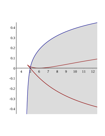
(a)  $q=5$  ($k=2$)

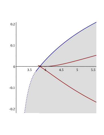
(b)  $q=3$  ($k=2$)

Figure 3. The phase diagram for the Potts model (2.30) showing the non-uniqueness region (shaded in grey) according to Theorem 2.10: (a) regular case $q\geq 4$ (shown here for $q=5$); (b) special case $q=3$, both with $k=2$. The critical boundaries are determined by (parts of) the graphs of the functions $\alpha_{\pm}(\theta)$ and $\alpha_{1}(\theta)$ defined in (2.41) and (2.46), respectively. The dotted part of the boundary on panel (b), given by $\alpha=\alpha_{1}(\theta)$, $\theta\in(\theta_{1},\tilde{\theta}_{1}]$ (see formula (2.50) with $q=3$), is excluded from the shaded region (see Theorem 2.10(b) and Conjecture 2.1, proved for $2\leq k\leq 4$); here, $\theta_{1}=3$ and $\tilde{\theta}_{1}=\frac{1}{2}\bigl{(}1+\sqrt{41}\mbox{$\>\!$}\bigr{)}\doteq 3.7016$.

To conclude this subsection, the following result describes a few cases where it is possible to estimate the maximal number of solutions of the system (2.31).

Theorem 2.11.

• If $q=2$ then $\nu(\theta,\alpha)\leq 3$; moreover, $\nu(\theta,\alpha)=3$ for all $\theta\geq 1$ large enough.

• Let $\alpha=0$ and $k\geq 2$. Then $\nu(\theta,0)\leq 2^{q}-1$ for all $\theta\geq 1$; moreover, $\nu(\theta,0)=2^{q}-1$ for all $\theta$ large enough.

• If $k=2$ then $\nu(\theta,\alpha)\leq 2^{q}-1$ for all $\theta\geq 1$ and $\alpha\in\mathbb{R}$.

Conjecture 2.2.

The upper bound $2^{q}-1$ in Theorem 2.11 appears to be universal. There is empirical evidence from exploration of many specific cases (using the computing package Maple) to conjecture that Theorem 2.11(c) holds true for all $k\geq 2$.

2.3.4. Some comments on earlier work

For $q=2$, when the Potts model is reduced to the Ising model, the result of Theorem 2.11(a) is well known (see [22, Section 12.2] or [47, Chapter 2]). The case $\alpha=0$ (i.e., with zero field) is also well studied (see, e.g., [47, Section 5.2.2.2, Proposition 5.4, pages 114–115] and [30, Theorem 1, page 192]), the result of Theorem 2.11(b) can be considered as a corollary of [30, Theorem 1, page 192]); in particular, it is known that there are $\bigl{\lfloor}\frac{1}{2}(q+1)\bigr{\rfloor}$ critical values of $\theta$, including $\theta_{0}^{-}=\theta_{1}^{\mbox{$\>\!$}0}$ and $\theta_{0}^{+}=1+q/(k-1)$.

The general case $q\geq 3$ with $\alpha\in\mathbb{R}$ was first addressed by Peruggi et al. [41] (and continued in [42]) using physical argumentation. In particular, they correctly identified the critical point $\theta_{\rm c}$ [42, equation (22), page 160] (cf. (2.35)) and also suggested an explicit critical boundary in the phase diagram for $\alpha\geq 0$, defined by the expression [42, equation (21), page 160] (adapted to our notation)

$$\tilde{\alpha}_{-}(\theta)=\frac{(k+1)\ln\bigl{(}1+(q-2)/\theta\bigr{)}-(k-1)\ln(q-1)}{2\ln\theta}.$$

Note that this function enjoys a correct value at $\theta=\theta_{\rm c}$ (i.e., $\tilde{\alpha}_{-}(\theta_{\rm c})=\alpha_{\pm}(\theta_{\rm c})$, see formula (6.4) below), but $\tilde{\alpha}_{-}(\theta)>\alpha_{-}(\theta)$ for all $\theta>\theta_{\rm c}$. The corresponding critical value of activity $\theta$, emerging as zero of $\tilde{\alpha}_{-}(\theta)$, is reported in [42, equation (20), page 158] as

$$\theta_{\rm cr}=\theta_{\rm cr}(k,q):=\frac{q-2}{(q-1)^{(k-1)/(k+1)}-1}.$$

In particular, $\theta_{\rm cr}$ is bigger than the exact critical value $\theta_{0}^{-}=\theta_{1}^{\mbox{$\>\!$}0}$, where the uniqueness breaks down at $\alpha=0$ (see Proposition 6.16). For example, the corresponding numerical values (for $k=5$ and $q=3$ or $q=8$) are given by (cf. [42, figure 1, page 159])

$$\theta_{\rm cr}\doteq\begin{cases}1.7024,&q=3,\\ 2.2562,&q=8,\end{cases}\qquad\theta_{0}^{-}\doteq\begin{cases}1.6966,&q=3,\\ 2.1803,&q=8.\end{cases}$$

The critical boundary in the phase diagram for $\alpha\leq 0$ was described in [42, page 160] only heuristically, as a line “joining” the points $\theta=\theta_{\rm cr}(k,q)$, $\alpha=0$ and $\theta=\theta_{\rm cr}(k,q-1)$, $\alpha=-\infty$, and illustrated by a sketch graph in the vicinity of $\theta_{\rm cr}(k,q)$ (for $k=5$ and $q=3$ or $q=8$).

It should be stressed that the phase transition occurring at these critical boundaries is not of type “uniqueness/non-uniqueness”, with which we are primarily concerned in the present paper, but in fact the so-called “order/disorder” phase transition. The latter was studied rigorously in a recent paper by Galanis et al. [18] in connection with the computational complexity of approximating the partition function of the Potts model. The useful classification of critical points deployed in [18] is based on the notion of dominant phase; in particular, the critical point $\theta_{0}^{+}=1+q/(k-1)$ (conjectured earlier by Häggström [26] in a more general context of random cluster measures on trees) can be explained from this point of view as a threshold beyond which only ordered phases are dominant. Note that the paper [18] studies the Potts model primarily with zero external field ($\alpha=0$); the authors claim that their methods should also work in a more general ferromagnetic framework including a non-zero field, but no details are spelled out clearly.

In the present paper, we do not investigate the thermodynamical nature of phase transitions, instead focussing on the number of completely homogeneous SGMs, especially on the uniqueness issue. In particular, the order/disorder critical point $\theta_{\rm cr}$ is not immediately detectable by our methods. It would be interesting to look into these issues for the Potts model with external field, thus extending the results of [18]. More specifically, our analysis (see Proposition 6.16) shows that the critical point $\theta_{0}^{+}$ is the signature of the upper critical function $\alpha_{+}(\theta)$ at $\alpha=0$, which has a minimum at $\theta=\theta_{0}^{+}$. Therefore, it is reasonable to conjecture that the $\alpha>0$ analogue of the interval of activities $\theta$ between the critical points $\theta_{0}^{-}$ and $\theta_{\rm cr}$ is the interval $[\theta_{\alpha}^{-},\theta_{\alpha}^{+}]$, where $\theta_{\alpha}^{-}$ is the (sole) root of the equation $\alpha_{-}(\theta)=\alpha$ and $\theta_{\alpha}^{+}$ is the smaller root of the similar equation $\alpha_{+}(\theta)=\alpha$. However, it is not clear as to what happens in the interval between the roots of the latter equation. The counterpart of this picture for $\alpha<0$ is likely to be simpler, as only the equation $\alpha_{-}(\theta)=\alpha$ is involved. We intend to address these issues in our forthcoming work.

3. Auxiliary lemmas

In this section, we collect a few technical results that will be instrumental in the proofs of the main theorems. We start with an elementary lemma.

Lemma 3.1.

For $a,b,c,d>0$, consider the function

$$f(t):=\ln\frac{a\mbox{$\>\!$}\mathrm{e}^{t}+b}{c\mbox{$\>\!$}\mathrm{e}^{t}+d},\qquad t\in\mathbb{R}.$$ (3.1)

• If $ad>bc$ then $f(t)$ is monotone increasing on $\mathbb{R}$ and

  $$\ln\frac{b}{d}\leq f(t)\leq\ln\frac{a}{c},\qquad t\in\mathbb{R}.$$ (3.2)

  Similarly, if $ad<bc$ then $f(t)$ is monotone decreasing on $\mathbb{R}$ and

  $$\ln\frac{a}{c}\leq f(t)\leq\ln\frac{b}{d},\qquad t\in\mathbb{R}.$$

• Furthermore,

  $$|f^{\prime}(t)|\leq\frac{|ad-bc|}{\bigl{(}\sqrt{ad}+\sqrt{bc}\mbox{$\>\!$}\bigr{)}^{2}},\qquad t\in\mathbb{R}.$$ (3.3)

Proof.

(a) Differentiating equation (3.1), we get

$$f^{\prime}(t)=\frac{a\mbox{$\>\!$}\mathrm{e}^{t}}{a\mbox{$\>\!$}\mathrm{e}^{t}+b}-\frac{c\mbox{$\>\!$}\mathrm{e}^{t}}{c\mbox{$\>\!$}\mathrm{e}^{t}+d}=\frac{ad-bc}{ac\mbox{$\;\!$}\mathrm{e}^{t}+bd\mbox{$\;\!$}\mathrm{e}^{-t}+ad+bc}.$$ (3.4)

If $ad>bc$ then, according to (3.4), the function $f(t)$ is monotone increasing, and the bounds (3.2) follow by taking the limit as $t\to\pm\infty$. The case $ad<bc$ is similar.

(b) By the inequality between the arithmetic and geometric means, the denominator on the right-hand side of (3.4) is bounded below by

$$2\sqrt{abcd}+ad+bc=\bigl{(}\sqrt{ad}+\sqrt{bc}\mbox{$\>\!$}\bigr{)}^{2},$$

and the result (3.3) follows. ∎

Let us define two norms for vector $u=(u_{1},\dots,u_{q-1})\in\mathbb{R}^{q-1}$,

$$\|u\|_{\infty}:=\max_{1\leq i\leq q-1}|u_{i}|,\qquad\|u\|_{1}:=\sum_{i=1}^{q-1}|u_{i}|.$$ (3.5)

The next two lemmas give useful estimates for the function $\boldsymbol{F}=(F_{1},\dots,F_{q-1})$ defined in (2.3) and for its partial derivatives.

Lemma 3.2.

For any $\theta\geq 1$, the following uniform estimate holds,

$$\sup_{u\in\smash{\mathbb{R}^{q-1}}}\|\boldsymbol{F}(u;\theta)\|_{\infty}\leq\ln\theta.$$ (3.6)

Proof.

Note that $F_{i}$, as a function of $u_{i}$, may be represented by formula (3.1) with the coefficients

$$a=\theta,\quad b=1+s,\quad c=1,\quad d=\theta+s,\quad s:=\sum_{j\neq i}\mathrm{e}^{u_{j}}\geq 0,$$ (3.7)

where

$$ad-bc=\theta\mbox{$\>\!$}(\theta+s)-(1+s)=(\theta-1)(\theta+1+s)>0.$$

Therefore, by the estimates (3.2) we have

$$\ln\frac{1+s}{\theta+s}\leq F_{i}(u;\theta)\leq\ln\theta.$$ (3.8)

Furthermore, noting that $(1+s)/(\theta+s)\geq 1/\theta$, the two-sided bound (3.8) implies the inequality $|F_{i}(u;\theta)|\leq\ln\theta$, and the bound (3.6) follows by taking the maximum over $i=1,\dots,q$. ∎

Recall that the function $\varphi(t;\theta)$ is defined by (2.4). Denote by $\nabla F_{i}$ the gradient of the map $\boldsymbol{u}\mapsto F_{i}(\boldsymbol{u};\theta)$,

$$\nabla F_{i}(\boldsymbol{u};\theta):=\left(\frac{\partial F_{i}(\boldsymbol{u};\theta)}{\partial u_{1}},\dots,\frac{\partial F_{i}(\boldsymbol{u};\theta)}{\partial u_{q-1}}\right),\qquad\boldsymbol{u}\in\mathbb{R}^{q-1}.$$

Recall that the norm $\|\mbox{$\>\!$}{\cdot}\mbox{$\>\!$}\|_{1}$ is defined in (3.5).

Lemma 3.3.

For $\gamma\in\mathbb{R}$ and any $\boldsymbol{u}=(u_{1},\dots,u_{q-1})\in\mathbb{R}^{q-1}$ such that $\min_{1\leq i\leq q-1}u_{i}\geq\gamma\ln\theta$, it holds

$$\max_{1\leq i\leq q-1}\|\nabla F_{i}(\boldsymbol{u};\theta)\|_{1}\leq Q(\theta)+\varphi(t_{\gamma}(\theta);\theta),$$ (3.9)

where $Q(\theta)$ is defined in (2.7) and $t_{\gamma}(\theta)=\theta+1+(q-2)\mbox{$\;\!$}\theta^{\gamma}$ (see (2.14)). Moreover, the following uniform estimate holds,

$$\max_{1\leq i\leq q-1}\sup_{\boldsymbol{u}\in\mathbb{R}^{q-1}}\|\nabla F_{i}(\boldsymbol{u};\theta)\|_{1}\leq Q(\theta)+\frac{\theta-1}{\theta+1}.$$ (3.10)

Proof.

Like in the proof of Lemma 3.2, let us represent $F_{i}(\boldsymbol{u};\theta)$ by formula (3.1) with the coefficients (3.7). Then by Lemma 3.1

$$\left|\frac{\partial F_{i}(\boldsymbol{u};\theta)}{\partial u_{i}}\right|\leq\frac{(\theta-1)(\theta+1+s)}{\bigl{(}\sqrt{\theta\mbox{$\>\!$}(\theta+s)}+\sqrt{1+s}\mbox{$\>\!$}\bigr{)}^{2}}=\varphi(\theta+1+s;\theta),$$ (3.11)

where $s=\sum_{j\neq i}\mathrm{e}^{u_{j}}\geq(q-2)\mbox{$\;\!$}\theta^{\gamma}=t_{\gamma}(\theta)-\theta-1$. Hence, by monotonicity of the map $t\mapsto\varphi(t;\theta)$, from (3.11) it follows that

$$\left|\frac{\partial F_{i}(\boldsymbol{u};\theta)}{\partial u_{i}}\right|\leq\varphi(t_{\gamma}(\theta);\theta).$$ (3.12)

On the other hand, expressing $F_{i}(\boldsymbol{u};\theta)$ by formula (3.1) with

$$a=1,\quad b=\theta\mbox{$\;\!$}\mathrm{e}^{u_{i}}+1+s^{\prime},\quad c=1,\quad d=\theta+\mathrm{e}^{u_{i}}+s^{\prime},\quad s^{\prime}:=\sum_{\ell\neq i,j}\mathrm{e}^{u_{\ell}}\geq 0,$$

by Lemma 3.1 we obtain

$$\left|\frac{\partial F_{i}(\boldsymbol{u};\theta)}{\partial u_{j}}\right| \leq\frac{(\theta-1)\mbox{$\>\!$}|\mathrm{e}^{u_{i}}-1|}{\bigl{(}\sqrt{\theta+\mathrm{e}^{u_{i}}+s^{\prime}}+\sqrt{\theta\mbox{$\>\!$}\mathrm{e}^{u_{i}}+1+s^{\prime}}\mbox{$\>\!$}\bigr{)}^{2}}.$$ (3.13)

If $u_{i}>0$ then the estimate (3.13) specializes to

$$\left|\frac{\partial F_{i}(\boldsymbol{u};\theta)}{\partial u_{j}}\right| \leq\frac{(\theta-1)(\mathrm{e}^{u_{i}}-1)}{\bigl{(}\sqrt{\theta+\mathrm{e}^{u_{i}}+s^{\prime}}+\sqrt{\theta\mbox{$\>\!$}\mathrm{e}^{u_{i}}+1+s^{\prime}}\mbox{$\>\!$}\bigr{)}^{2}}$$

$$\leq\frac{\theta-1}{\bigl{(}\sqrt{1+(\theta+1)/(\mathrm{e}^{u_{i}}-1)}+\sqrt{\theta+(\theta+1)/(\mathrm{e}^{u_{i}}-1)}\mbox{$\>\!$}\bigr{)}^{2}}$$

$$\leq\frac{\theta-1}{(\sqrt{1}+\sqrt{\theta}\mbox{$\>\!$})^{2}}=\frac{\sqrt{\theta}-1}{\sqrt{\theta}+1}.$$ (3.14)

Similarly, if $u_{i}\leq 0$ then $1\geq\mathrm{e}^{u_{i}}>0$ and from (3.13) we obtain

$$\left|\frac{\partial F_{i}(\boldsymbol{u};\theta)}{\partial u_{j}}\right| \leq\frac{(\theta-1)\mbox{$\>\!$}(1-\mathrm{e}^{u_{i}})}{\bigl{(}\sqrt{\theta+\mathrm{e}^{u_{i}}+s^{\prime}}+\sqrt{\theta\mbox{$\>\!$}\mathrm{e}^{u_{i}}+1+s^{\prime}}\mbox{$\>\!$}\bigr{)}^{2}}$$

$$\leq\frac{\theta-1}{(\sqrt{\theta}+\sqrt{1}\mbox{$\>\!$})^{2}}=\frac{\sqrt{\theta}-1}{\sqrt{\theta}+1}.$$ (3.15)

Thus, combining (3.14) and (3.15), we have

$$\left|\frac{\partial F_{i}(\boldsymbol{u};\theta)}{\partial u_{j}}\right|\leq\frac{\sqrt{\theta}-1}{\sqrt{\theta}+1},\qquad i\neq j.$$ (3.16)

As a result, according to the definition (3.5) of the norm $\|\cdot\|_{1}$, the bounds (3.12) and (3.16) imply the estimate (3.9).

Finally, since

$$\lim_{\gamma\to-\infty}\varphi(t_{\gamma}(\theta);\theta)=\varphi(\theta+1;\theta)=\frac{\theta-1}{\theta+1},$$ (3.17)

from (3.9) we obtain (3.10), and the proof of Lemma 3.3 is complete. ∎

Remark 3.1.

Estimates similar to (3.9) were proved in [49].

Lemma 3.4.

For integer $q\geq 2$ and any $\gamma\in\mathbb{R}$, the map $[1,\infty)\ni\theta\mapsto\varphi(t_{\gamma}(\theta);\theta)$ is a continuous, strictly increasing function with the range $[0,1)$.

Proof.

Denoting $\tilde{q}:=q-2\in\mathbb{N}_{0}$, by formula (2.5) we have

$$\varphi(t_{\gamma}(\theta);\theta)=\varphi(\theta+1+\tilde{q}\mbox{$\;\!$}\theta^{\gamma};\theta) =\frac{\sqrt{\theta\mbox{$\>\!$}(\theta+\tilde{q}\mbox{$\;\!$}\theta^{\gamma})}-\sqrt{1+\tilde{q}\mbox{$\;\!$}\theta^{\gamma}}}{\sqrt{\theta\mbox{$\>\!$}(\theta+\tilde{q}\mbox{$\;\!$}\theta^{\gamma})}+\sqrt{1+\tilde{q}\mbox{$\;\!$}\theta^{\gamma}}}$$

$$=1-2\left(1+\sqrt{\frac{\theta^{2}+\tilde{q}\mbox{$\;\!$}\theta^{\gamma+1}}{1+\tilde{q}\mbox{$\;\!$}\theta^{\gamma}}}\,\right)^{\!-1}.$$ (3.18)

Clearly, the function (3.18) is continuous, so we only need to show that

$$A(\theta):=\frac{\theta^{2}+\tilde{q}\mbox{$\;\!$}\theta^{\gamma+1}}{1+\tilde{q}\mbox{$\;\!$}\theta^{\gamma}},\qquad\theta\geq 1,$$ (3.19)

is an increasing function.

First of all, if $\tilde{q}=0$ then (3.19) is reduced to $A(\theta)=\theta^{2}$, so there is nothing to prove. Suppose that $\tilde{q}\geq 1$. Differentiating (3.19), it is easy to see that

$$A^{\prime}(\theta)=\frac{2\mbox{$\>\!$}\theta+\tilde{q}\mbox{$\;\!$}\theta^{\gamma}\bigl{[}\theta+2+\tilde{q}\mbox{$\;\!$}\theta^{\gamma}+(1-\gamma)(\theta-1)\bigr{]}}{\bigl{(}1+\tilde{q}\mbox{$\;\!$}\theta^{\gamma}\bigr{)}^{2}},$$ (3.20)

and it is evident that the right-hand side of (3.20) is positive for all $\theta\geq 1$ as long as $\gamma\leq 1$. On the other hand, for $\gamma\geq 1$ by Bernoulli’s inequality we have

$$\tilde{q}\mbox{$\;\!$}\theta^{\gamma}\geq\theta^{\gamma}=\bigl{(}1+(\theta-1)\bigr{)}^{\gamma}\geq 1+\gamma\mbox{$\;\!$}(\theta-1),$$

and the expression in square brackets in (3.20) is estimated from below by $(\theta+2)+1+(\theta-1)=2\mbox{$\>\!$}\theta+2>0$. Thus, in all cases $A^{\prime}(\theta)>0$ for $\theta\geq 1$, as required.

Finally, from (3.19) we see that $A(1)=1$ and $\lim_{\theta\to\infty}A(\theta)=\infty$, and it follows that the range of the function (3.18) is $[0,1)$, which completes the proof of the lemma. ∎

Lemma 3.5.

For $k\geq 2$, $q\geq 2$ and any $\gamma\in\mathbb{R}$, the equation (2.13) has a unique root $\theta^{*}_{\mbox{$\;\!\!$}\gamma}=\theta^{*}_{\mbox{$\;\!\!$}\gamma}(k,q)$. If $q=2$ then $\theta^{*}_{\mbox{$\;\!\!$}\gamma}(k,2)\equiv\theta_{0}(k,2)=(k+1)/(k-1)$, where $\theta_{0}(k,q)$ is the root of the equation (2.9). For $q\geq 3$, the root $\theta^{*}_{\mbox{$\;\!\!$}\gamma}$ is a continuous monotone increasing function of $\gamma$, such that

$$\lim_{\gamma\to-\infty}\theta^{*}_{\mbox{$\;\!\!$}\gamma}(k,q)=\theta_{0}(k,q),\qquad\lim_{\gamma\to+\infty}\theta^{*}_{\mbox{$\;\!\!$}\gamma}(k,q)=\left(\theta_{*}(k,q)\right)^{2},$$ (3.21)

where $\theta_{*}(k,q)$ is the root of the equation (2.12); in particular,

$$\theta_{0}(k,q)<\theta^{*}_{\mbox{$\;\!\!$}\gamma}(k,q)<\left(\theta_{*}(k,q)\right)^{2}.$$ (3.22)

Proof.

The case $q=2$ is straightforward, so assume that $q\geq 3$. Due to continuity and monotonicity of the function $Q(\theta)$ (see (2.7)) and by virtue of Lemma 3.4, the left-hand side of equation (2.13) is a continuous increasing function of $\theta\in[1,\infty)$, with the range $[0,q-1)$ because

$$\lim_{\theta\downarrow 1}\bigl{(}Q(\theta)+\varphi(t_{\gamma}(\theta);\theta)\bigr{)}=0,\qquad\lim_{\theta\to\infty}\bigl{(}Q(\theta)+\varphi(t_{\gamma}(\theta);\theta)\bigr{)}=q-1.$$

Hence, the equation (2.13) always has a unique solution, $\theta^{*}_{\mbox{$\;\!\!$}\gamma}=\theta^{*}_{\mbox{$\;\!\!$}\gamma}(k,q)$. Since $t_{\gamma}(\theta)$ is a continuous increasing function of $\gamma$, while the map $t\mapsto\varphi(t;\theta)$ is continuous and decreasing, it follows that the root $\theta^{*}_{\mbox{$\;\!\!$}\gamma}$ is continuous and increasing in $\gamma$.

Finally, observing that (see (2.6) and (3.17))

$$\lim_{\gamma\to-\infty}\varphi(t_{\gamma}(\theta);\theta)=\varphi(\theta+1;\theta)=\frac{\theta-1}{\theta+1},\qquad\lim_{\gamma\to\infty}\varphi(t_{\gamma}(\theta);\theta)=\varphi(\infty;\theta)=\frac{\sqrt{\theta}-1}{\sqrt{\theta}+1},$$

and comparing equation (2.13) with the limiting equations as $\gamma\to\pm\infty$ (which have the roots $\theta_{0}$ and $\theta_{*}^{2}$, respectively), we obtain the required limits (3.21), and hence the asymptotic bounds (3.22) for $\theta^{*}_{\mbox{$\;\!\!$}\gamma}$. ∎

4. Proofs of the main results related to uniqueness

4.1. Proof of Theorem 2.1 (criterion of compatibility)

For shorthand, denote temporarily $\boldsymbol{\zeta}(x):=\boldsymbol{h}(x)+\boldsymbol{\xi}(x)$. Suppose that the compatibility condition (1.8) holds. On substituting (1.6), it is easy to see that (1.8) simplifies to

$$\prod_{x\in W_{n}}\prod_{y\in S(x)}\sum_{\omega(y)\in\varPhi}\exp\bigl{\{}\beta\bigl{(}J_{xy}\mbox{$\;\!$}\delta_{\sigma_{n}(x),\mbox{$\;\!$}\omega(y)}+\zeta_{\omega(y)}(y)\bigr{)}\bigr{\}}=\frac{Z_{n+1}}{Z_{n}}\prod_{x\in W_{n}}\exp\bigl{\{}\beta h_{\sigma_{n}(x)}(x)\bigr{\}},$$ (4.1)

for any $\sigma_{n}\in\varPhi^{V_{n}}$. Consider the equality (4.1) on configurations $\sigma_{n}^{1},\sigma_{n}^{2}\in\varPhi^{V_{n}}$ that coincide everywhere in $V_{n}$ except at vertex $x\in W_{n}$, where $\sigma_{n}^{1}(x)=i\leq q-1$ and $\sigma_{n}^{2}(x)=q$. Taking the log-ratio of the two resulting relations, we obtain

$$\sum_{y\in S(x)}\ln\frac{\exp\bigl{\{}\beta\bigl{(}J_{xy}+\zeta_{i}(y)\bigr{)}\bigr{\}}+\sum_{j\neq i}\exp\bigl{\{}\beta\mbox{$\>\!$}\zeta_{j}(y)\bigr{\}}}{\exp\bigl{\{}\beta\bigl{(}J_{xy}+\zeta_{q}(y)\bigr{)}\bigr{\}}+\sum_{j=1}^{q-1}\exp\bigl{\{}\beta\mbox{$\>\!$}\zeta_{j}(y)\bigr{\}}}=\beta\bigl{(}h_{i}(x)-h_{q}(x)\bigr{)},$$

which is readily reduced to (2.1) in view of the notation (2.2) and (2.3).

Conversely, again using (2.2) and (2.3), equation (2.1) can be rewritten in the coordinate form as follows,

$$\prod_{y\in S(x)}\sum_{j=1}^{q}\exp\bigl{\{}\beta\bigl{(}J_{xy}\mbox{$\;\!$}\delta_{ij}+\zeta_{j}(y)\bigr{)}\bigr{\}}=a(x)\exp\{\beta h_{i}(x)\},\qquad i=1,\dots,q-1,$$ (4.2)

where (omitting the immaterial dependence on $\beta$, $\boldsymbol{h}$ and $\boldsymbol{\xi}$) we denote

$$a(x):=\exp\{\beta h_{q}(x)\}\prod_{y\in S(x)}\sum_{j=1}^{q}\exp\bigl{\{}\beta\bigl{(}J_{xy}\mbox{$\;\!$}\delta_{qj}+\zeta_{j}(y)\bigr{)}\bigr{\}},\qquad x\in V.$$

Hence, using (4.2) and setting $A_{n}:=\prod_{x\in W_{n}}a(x)$, we get

$$\sum_{\omega\in\varPhi^{W_{n+1}}}\mu^{h}_{n+1}(\sigma_{n}\mbox{$\>\!\!$}\vee\omega) =\frac{\exp\{-\beta H_{n}(\sigma_{n})\}}{Z_{n+1}}\prod_{x\in W_{n}}\prod_{y\in S(x)}\sum_{j=1}^{q}\exp\bigl{\{}\beta\bigl{(}J_{xy}\mbox{$\;\!$}\delta_{\sigma_{n}(x),\mbox{$\>\!$}j}+\zeta_{j}(y)\bigr{)}\bigr{\}}$$

$$=\frac{A_{n}}{Z_{n+1}}\exp\left\{-\beta H_{n}(\sigma_{n})+\beta\sum_{x\in W_{n}}h_{\sigma_{n}(x)}(x)\right\}=\frac{A_{n}Z_{n}}{Z_{n+1}}\mu_{n}^{h}(\sigma_{n}).$$ (4.3)

Finally, observe that

$$\sum_{\sigma_{n}\in\varPhi^{V_{n}}}\sum_{\omega\in\varPhi^{W_{n+1}}}\mu_{n+1}^{h}(\sigma_{n}\mbox{$\>\!\!$}\vee\omega)=\sum_{\sigma_{n+1}\in\varPhi^{V_{n+1}}}\mu_{n+1}^{h}(\sigma_{n+1})=1,$$

whereas from the right-hand side of (4.3) the same sum is given by

$$\sum_{\sigma_{n}\in\varPhi^{V_{n}}}\frac{A_{n}Z_{n}}{Z_{n+1}}\mu_{n}^{h}(\sigma_{n})=\frac{A_{n}Z_{n}}{Z_{n+1}}.$$

Hence, $A_{n}Z_{n}/Z_{n+1}=1$ and formula (4.3) yields (1.8), as required. This completes the proof of Theorem 2.1.

4.2. Preparatory results for the uniqueness of SGM

First, let us rewrite the functional equation (2.1) in a form more convenient for iterations. Recall that we assume $J_{xy}\equiv J>0$ ($d(x,y)=1$) and use the notation $\theta=\mathrm{e}^{\beta J}$.

Lemma 4.1.

Via the substitutions

$$\boldsymbol{g}(x)=\boldsymbol{F}\bigl{(}\beta\mbox{$\>\!$}\boldsymbol{\check{h}}(x)+\beta\mbox{$\>\!$}\boldsymbol{\check{\xi}}(x);\theta\bigr{)}\in\mathbb{R}^{q-1},\qquad x\in V,$$ (4.4)

and

$$\boldsymbol{\check{h}}(x)=\beta^{-1}\!\sum_{y\in S(x)}\boldsymbol{g}(y),\qquad x\in V,$$ (4.5)

equation (2.1) is equivalent to the fixed-point equation

$$\boldsymbol{g}(x)=\boldsymbol{\varPsi}\boldsymbol{g}(x),\qquad x\in V,$$ (4.6)

where the mapping $\boldsymbol{\varPsi}\colon(\mathbb{R}^{q-1})^{V}\to(\mathbb{R}^{q-1})^{V}$ is defined by

$$\boldsymbol{\varPsi}\boldsymbol{g}(x):=\boldsymbol{F}\!\left(\beta\mbox{$\>\!$}\boldsymbol{\check{\xi}}(x)+\sum_{\smash{y\in S(x)}}\boldsymbol{g}(y);\theta\right),\qquad x\in V.$$ (4.7)

Proof.

By means of (4.4), the recursive equation (2.1) for $\boldsymbol{\check{h}}$ can be written as (4.5). Substituting this into (4.4) and using the notation (4.7), we see that $\boldsymbol{g}$ solves the functional equation (4.6). Conversely, if $\boldsymbol{g}$ satisfies the equation (4.6) then for $\boldsymbol{\check{h}}$ defined by (4.5) we have, using (4.7),

$$\beta\mbox{$\>\!$}\boldsymbol{\check{h}}(x)=\sum_{y\in S(x)}\boldsymbol{g}(y) =\sum_{y\in S(x)}\boldsymbol{\varPsi}\boldsymbol{g}(y)$$

$$=\sum_{y\in S(x)}\boldsymbol{F}\!\left(\beta\mbox{$\>\!$}\boldsymbol{\check{\xi}}(y)+\sum_{\smash{z\in S(y)}}\boldsymbol{g}(z);\theta\right)$$

$$=\sum_{y\in S(x)}\boldsymbol{F}\!\left(\beta\mbox{$\>\!$}\boldsymbol{\check{\xi}}(y)+\beta\mbox{$\>\!$}\boldsymbol{\check{h}}(y);\theta\right),$$

so that $\boldsymbol{\check{h}}$ solves the equation (2.1). Thus, Lemma 4.1 is proved. ∎

In particular, Lemma 4.1 implies that for the proof of uniqueness of SGM it suffices to show that the equation (4.6) has a unique solution $\boldsymbol{g}(x)$ ($x\in V$).

Let us state and prove one general result in the contraction case. On the vector space $(\mathbb{R}^{q-1})^{V}\!$ of $\mathbb{R}^{q-1}$-valued functions on the vertex set $V$ of the Cayley tree $\mathbb{T}^{k}$, introduce the $\sup$-norm

$$\|\boldsymbol{g}\|_{V}:=\sup_{x\in V}\|\boldsymbol{g}(x)\|_{\infty}=\sup_{x\in V}\max_{1\leq i\leq q-1}|g_{i}(x)|,\qquad\boldsymbol{g}(x)=(g_{1}(x),\dots,g_{q-1}(x)).$$

Sometimes, we need the similar norm for functions restricted to subsets $\varLambda\subseteq V$,

$$\|\boldsymbol{g}\|_{\varLambda}:=\sup_{x\in\varLambda}\|\boldsymbol{g}(x)\|_{\infty},\qquad\boldsymbol{g}\in(\mathbb{R}^{q-1})^{\varLambda}\!.$$ (4.8)

The next lemma and its proof are an adaptation of a standard result for $\ell^{\infty}(\mathbb{R})$.

Lemma 4.2.

For any subset $\varLambda\subseteq V$, the space $(\mathbb{R}^{q-1})^{\varLambda}$ is complete with respect to the sup-norm (4.8).

Proof.

Let $\{\boldsymbol{g}^{n}\}$ be a Cauchy sequence in $(\mathbb{R}^{q-1})^{\varLambda}\!$, that is, for any $\varepsilon>0$ there is $N\in\mathbb{N}$ such that for any $n,m\geq N$ we have $\|\boldsymbol{g}^{n}-\boldsymbol{g}^{m}\|_{\varLambda}<\varepsilon$. In particular, $\{\boldsymbol{g}^{n}\}$ is bounded, $\|\boldsymbol{g}^{n}\|_{\varLambda}\!\leq M<\infty$ for some $M>0$ and all $n\in\mathbb{N}$. Note that every coordinate sequence $\{g^{n}_{i}(x)\}$ ($i=1,\dots,q-1$, $x\in\varLambda$) is also a Cauchy sequence (in $\mathbb{R}$) because, according to (3.5), $|g^{n}_{i}(x)-g^{m}_{i}(x)|\leq\|\boldsymbol{g}^{n}-\boldsymbol{g}^{m}\|_{\varLambda}<\varepsilon$; hence, it converges to a limit which we denote $g_{i}(x)$. Clearly, $|g_{i}(x)|\leq M$ and $\|\boldsymbol{g}\|_{\varLambda}\!=\sup_{x\in\varLambda}\max_{i}|g_{i}(x)|\leq M<\infty$.

Now, passing to the limit as $m\to\infty$ in each inequality $|g^{n}_{i}(x)-g^{m}_{i}(x)|<\varepsilon$, we obtain $|g^{n}_{i}(x)-g_{i}(x)|\leq\varepsilon$, which implies that $\|\boldsymbol{g}^{n}-\boldsymbol{g}\|_{\varLambda}\!\leq\varepsilon$, for all $n\geq N$. Since $\varepsilon>0$ is arbitrary, we conclude that $\|\boldsymbol{g}^{n}-\boldsymbol{g}\|_{\varLambda}\!\to 0$ as $n\to\infty$, and the lemma is proved. ∎

We also require the following simple estimate.

Lemma 4.3.

Let $f(\boldsymbol{u})\colon\mathbb{R}^{q-1}\!\to\mathbb{R}$ be a $C^{1}$-function and $\nabla f(\boldsymbol{u})=\bigl{(}\frac{\partial f(\boldsymbol{u})}{\partial u_{1}},\dots,\frac{\partial f(\boldsymbol{u})}{\partial u_{q-1}}\bigr{)}$ its gradient. Then, for any $\boldsymbol{v},\boldsymbol{w}\in\mathbb{R}^{q-1}$,

$$|f(\boldsymbol{w})-f(\boldsymbol{v})|\leq\|\boldsymbol{w}-\boldsymbol{v}\|_{\infty}\,\sup_{\boldsymbol{u}\in\smash{\mathbb{R}^{q-1}}}\|\nabla f(\boldsymbol{u})\|_{1}.$$ (4.9)

Proof.

Define the function $\psi(t):=f(\boldsymbol{v}+t\mbox{$\>\!$}(\boldsymbol{w}-\boldsymbol{v}))$, $t\in[0,1]$, then

$$f(\boldsymbol{w})-f(\boldsymbol{v})=\psi(1)-\psi(0)=\int_{0}^{1}\psi^{\prime}(t)\,\mathrm{d}{t}=\int_{0}^{1}\sum_{i=1}^{q-1}\frac{\partial f(\boldsymbol{v}+t\mbox{$\>\!$}(\boldsymbol{w}-\boldsymbol{v}))}{\partial u_{i}}\mbox{$\;\!$}(w_{i}-v_{i})\,\mathrm{d}{t},$$

whence the estimate (4.9) readily follows. ∎

Theorem 4.4.

Suppose that, for some $\theta>1$,

$$\lambda(\theta):=k\max_{1\leq i\leq q-1}\sup_{\boldsymbol{u}\in\smash{\mathbb{R}^{q-1}}}\|\nabla F_{i}(\boldsymbol{u};\theta)\|_{1}<1.$$ (4.10)

Then, for every realization of the field $\boldsymbol{\xi}=\{\boldsymbol{\xi}(x)\}_{x\in V}$, the equation (4.6) has a unique solution.

Proof.

Consider a mapping $\boldsymbol{\varPsi}=(\varPsi_{1},\dots,\varPsi_{q-1})$ of the space $(\mathbb{R}^{q-1})^{V}$ to itself defined by formula (4.7). Solving the functional equation (4.6) is then equivalent to finding a fixed point of $\boldsymbol{\varPsi}$, that is, $\boldsymbol{\varPsi}\boldsymbol{g}^{*}=\boldsymbol{g}^{*}$. The lemma’s hypothesis implies that $\boldsymbol{\varPsi}$ is a contraction on $(\mathbb{R}^{q-1})^{V_{0}^{c}}$; indeed, for any functions $\boldsymbol{g},\bar{\boldsymbol{g}}\in(\mathbb{R}^{q-1})^{V}$ and each $i=1,\dots,q-1$, we obtain, using (4.7) and Lemma 4.3,

$$|\varPsi_{i}\mbox{$\>\!$}\boldsymbol{g}(x)-\varPsi_{i}\mbox{$\>\!$}\bar{\boldsymbol{g}}(x)| \leq\sup_{\boldsymbol{u}\in\smash{\mathbb{R}^{q-1}}}\|\nabla F_{i}(\boldsymbol{u};\theta)\|_{1}\sum_{y\in S(x)}\|\boldsymbol{g}(y)-\bar{\boldsymbol{g}}(y)\|_{\infty}.$$

Noting that for $x\neq x_{\circ}$ the set $S(x)$ contains exactly $k$ vertices, and recalling condition (4.10) with $\lambda(\theta)\in[0,1)$, it follows that

$$\|\boldsymbol{\varPsi}\boldsymbol{g}-\boldsymbol{\varPsi}\mbox{$\>\!$}\bar{\boldsymbol{g}}\|_{V_{0}^{c}} =\sup_{x\in V_{0}^{c}}\|\boldsymbol{\varPsi}\boldsymbol{g}(x)-\boldsymbol{\varPsi}\mbox{$\>\!$}\bar{\boldsymbol{g}}(x)\|_{\infty}$$

$$\leq\max_{1\leq i\leq q-1}\sup_{\boldsymbol{u}\in\smash{\mathbb{R}^{q-1}}}\|\nabla F_{i}(\boldsymbol{u};\theta)\|_{1}\cdot k\mbox{$\;\!$}\|\boldsymbol{g}-\bar{\boldsymbol{g}}\|_{V_{0}^{c}}=\lambda(\theta)\,\|\boldsymbol{g}-\bar{\boldsymbol{g}}\|_{V_{0}^{c}}.$$

Thus, because $(\mathbb{R}^{q-1})^{V_{0}^{c}}$ is a Banach space (Lemma 4.2), the well-known Banach contraction principle (e.g., [51, Theorem 9.23, page 220]) implies that $\|\boldsymbol{g}-\bar{\boldsymbol{g}}\|_{V_{0}^{c}}=0$, that is, $\boldsymbol{g}(x)=\bar{\boldsymbol{g}}(x)$ for all $x\in V_{0}^{c}$. It remains to notice that the value of the solution $\boldsymbol{g}(x)$ at $x=x_{\circ}$ is uniquely determined from formulas (4.6) and (4.7) using the (unique) values outside $V_{0}=\{x_{\circ}\}$. This completes the proof of Theorem 4.4. ∎

Remark 4.1.

The unique solution $\boldsymbol{g}^{*}$ can be obtained by iterations [51]; for example, put $\boldsymbol{g}^{0}\equiv\boldsymbol{0}$ and define $\boldsymbol{g}^{n}\!:=\boldsymbol{\varPsi}\boldsymbol{g}^{n-1}$ ($n\in\mathbb{N}$), then $\boldsymbol{g}^{n}\to\boldsymbol{g}^{*}$ as $n\to\infty$ (i.e., $\lim_{n\to\infty}{\|\boldsymbol{g}^{n}-\boldsymbol{g}^{*}\|_{V}=0}$).

Remark 4.2.

It is straightforward to generalize Theorem 4.4 to the case where the vector $\beta\mbox{$\>\!$}\boldsymbol{\check{\xi}}(x)+\sum_{y\in S(x)}\boldsymbol{g}(y)$ (see (4.7)) is guaranteed to be in a convex domain $B(x)\subseteq\mathbb{R}^{q-1}$ for any function $\boldsymbol{g}\colon V\to\mathbb{R}^{q-1}$ from a suitable subspace $\mathscr{D}\subseteq(\mathbb{R}^{q-1})^{V}$, such that $\mathscr{D}$ is closed with respect to the norm $\|\mbox{$\;\!$}{\cdot}\mbox{$\;\!$}\|_{V}$ and $\boldsymbol{\varPsi}(\mathscr{D})\subseteq\mathscr{D}$ . In that case, the supremum in (4.10) should be taken over all $\boldsymbol{u}\in B(x)$,

$$\lambda(\theta):=k\sup_{x\in V}\max_{1\leq i\leq q-1}\sup_{\boldsymbol{u}\in B(x)}\|\nabla F_{i}(\boldsymbol{u};\theta)\|_{1}<1,$$

and the unique solution $\boldsymbol{g}^{*}$ automatically belongs to $\mathscr{D}\mbox{$\>\!\!$}$. For our purposes, it will suffice to consider the balls $B(x)=\{\boldsymbol{u}\in\mathbb{R}^{q-1}\colon\|\boldsymbol{u}-\beta\mbox{$\>\!$}\boldsymbol{\check{\xi}}(x)\|_{\infty}\leq k\ln\theta\}$ and the corresponding subspace $\mathscr{D}=\{\boldsymbol{g}\in(\mathbb{R}^{q-1})^{V}\colon\,\|\boldsymbol{g}\|_{V}\leq\ln\theta\}$ (see Lemma 3.2).

4.3. Proofs of Theorems 2.2, 2.3 and 2.5 (uniqueness)

By virtue of Remark 1.5, for the uniqueness in the class of all Gibbs measure it suffices to prove it for SGMs.

4.3.1. Proof of Theorem 2.2

By virtue of the uniform bound (3.10) of Lemma 3.3, for every $\theta\in[1,\theta_{0})$ we have

$$\lambda(\theta)=k\max_{1\leq i\leq q-1}\sup_{\boldsymbol{u}\in\smash{\mathbb{R}^{q-1}}}\|\nabla F_{i}(\boldsymbol{u};\theta)\|_{1}\leq k\left(Q(\theta)+\frac{\theta-1}{\theta+1}\right)<1,$$

and the required result follows by Theorem 4.4.

4.3.2. Proof of Theorem 2.3

In view of equation (2.13) with $\gamma=\varDelta^{\xi}-k$, we have

$$Q(\theta)+\varphi\bigl{(}t_{\mbox{$\;\!\!$}\varDelta^{\xi}-k}(\theta);\theta\bigr{)}<\frac{1}{k},\qquad\theta\in[1,\theta^{*}_{\mbox{$\>\!\!$}\varDelta^{\xi}-k}).$$ (4.11)

By continuity of the map $\gamma\mapsto\varphi(t_{\gamma}(\theta);\theta)$, inequality (4.11) extends to

$$Q(\theta)+\varphi\bigl{(}t_{\mbox{$\;\!\!$}\varDelta^{\xi}-\delta-k}(\theta);\theta\bigr{)}<\frac{1}{k},$$ (4.12)

for some $\delta>0$ small enough.

According to the definition (2.16), there exists an integer $N$ such that

$$\max_{1\leq\ell\leq q}\inf_{x\in V_{\mbox{$\;\!\!$}N}^{c}}{}_{\ell}\check{\xi}_{(1)}(x)\geq\varDelta^{\xi}-\delta.$$ (4.13)

For a specific reduction ${}_{\ell\mbox{$\>\!$}}\boldsymbol{\check{\xi}}(x)\!\in\!{}_{\ell}\check{\mathbb{R}}^{q}$, with components ${}_{\ell}\check{\xi}_{j}(x)=\xi_{j}(x)-\xi_{\ell}(x)$ ($j\neq\ell$), denote by ${}_{\ell}F_{i}(\boldsymbol{u};\theta)$ ($i\neq\ell$) the corresponding functions analogous to $F_{i}(\boldsymbol{u};\theta)$ that were defined in (2.3) under the standard reduction (i.e., with $\ell=q$). Lemma 3.3 (modified to the case of reduction via the $\ell$-th coordinate) implies that

$$\max_{i\neq\ell}\sup_{\boldsymbol{u}\in B_{\ell}(x)}\|\nabla{}_{\ell}F_{i}(\boldsymbol{u};\theta)\|_{1}\leq Q(\theta)+\varphi\bigl{(}t_{\mbox{$\;\!\!$}{}_{\ell}\check{\xi}_{(1)}(x)-k}(\theta);\theta\bigr{)},$$ (4.14)

where

$$B_{\ell}(x):={} \!\Bigl{\{}\boldsymbol{u}\in{}_{\ell}\check{\mathbb{R}}^{q}\!:\,\min_{j\neq\ell}u_{j}\geq\bigl{(}{}_{\ell}\mbox{$\>\!$}\check{\xi}_{(1)}(x)-k\bigr{)}\ln\theta\Bigr{\}}.$$

Furthermore, exploiting monotonicity and continuity of the function $t\mapsto\varphi(t;\theta)$, we obtain from (4.14)

$$\min_{1\leq\ell\leq q}\sup_{x\in V_{\mbox{$\;\!\!$}N}^{c}}\max_{i\neq\ell}\sup_{\boldsymbol{u}\in B_{\ell}(x)}\|\nabla{}_{\ell}F_{i}(\boldsymbol{u};\theta)\|_{1} \leq Q(\theta)+\varphi\bigl{(}t^{*}_{N}(\theta);\theta\bigr{)},$$ (4.15)

with

$$t^{*}_{N}(\theta):=\max_{1\leq\ell\leq q}\,\inf_{x\in V_{\mbox{$\;\!\!$}N}^{c}}t_{\mbox{$\;\!\!$}{}_{\ell}\check{\xi}_{(1)}(x)-k}(\theta).$$

Due to the bound (4.13), we have $t^{*}_{N}(\theta)\geq t_{\mbox{$\;\!\!$}\varDelta^{\xi}-\delta-k}(\theta)$, and by monotonicity of $t\mapsto\varphi(t;\theta)$ it follows that

$$Q(\theta)+\varphi\bigl{(}t^{*}_{N}(\theta);\theta\bigr{)}\leq Q(\theta)+\varphi\bigl{(}t_{\mbox{$\;\!\!$}\varDelta^{\xi}-\delta-k}(\theta);\theta\bigr{)}<\frac{1}{k},$$

according to the estimate (4.12). Together with (4.15), this implies that (cf. condition (4.10))

$$\lambda_{N}(\theta):=k\min_{1\leq\ell\leq q}\sup_{x\in V_{\mbox{$\;\!\!$}N}^{c}}\max_{i\neq\ell}\sup_{\boldsymbol{u}\in B_{\ell}(x)}\|\nabla_{\ell}F_{i}(\boldsymbol{u};\theta)\|_{1}<1.$$

Hence, by an extended version of Theorem 4.4 (see Remark 4.2), it follows that the solution $\boldsymbol{g}(x)$ to the functional equation (4.6) is unique on the subset $\{x\in V_{\mbox{$\;\!\!$}N}^{c}\}$. Finally, the values of the solution $\boldsymbol{g}(x)$ for $x\in V_{N}$ are retrieved uniquely by the “backward” recursion (4.6) using (4.7). Thus, the proof of Theorem 2.3 is complete.

4.3.3. Proof of Theorem 2.5

Let $\mu_{\beta,\mbox{$\>\!$}\xi}$ and $\bar{\mu}_{\beta,\mbox{$\>\!$}\xi}$ be two SGMs determined by the functions $\boldsymbol{g}(x)$ and $\bar{\boldsymbol{g}}(x)$, respectively, each satisfying the functional equation (4.6). Our aim is to show that, under the theorem’s hypotheses, $\boldsymbol{g}(x)\equiv\bar{\boldsymbol{g}}(x)$, which would imply that $\mu_{\beta,\mbox{$\>\!$}\xi}=\bar{\mu}_{\beta,\mbox{$\>\!$}\xi}$. The idea of the proof is to obtain a suitable upper bound on the norm $\|\boldsymbol{g}(x)-\bar{\boldsymbol{g}}(x)\|_{\infty}$ for $x\in W_{n}$ in terms of $\|\boldsymbol{g}(y)-\bar{\boldsymbol{g}}(y)\|_{\infty}$ for $y\in W_{n+1}$, and to propagate this estimate along the tree. To circumvent cumbersome notation arising from the direct iterations, we will use mathematical induction. Consider the filtration $\mathscr{F}_{0}\subset\mathscr{F}_{1}\subset\dots\mathscr{F}_{n}\subset\cdots$ consisting of the sigma-algebras $\mathscr{F}_{n}$ generated by the values of the random field $\boldsymbol{\xi}$ in the sequence of expanding balls $V_{n}=\{x\in V\colon d(x_{\circ},x)\leq n\}$,

$$\mathscr{F}_{n}:=\sigma\{\boldsymbol{\xi}(x)\colon x\in V_{n}\},\qquad n\in\mathbb{N}_{0}.$$

Put

$$\lambda(\theta):=k\,\bigl{(}Q(\theta)+\mathbb{E}\bigl{[}\varphi\bigl{(}t_{\check{\xi}_{(1)}(x)-k}(\theta);\theta\bigr{)}\bigr{]}\bigr{)},$$ (4.16)

where the expectation does not depend on $x\in V$ due to the i.i.d. assumption on the field $\{\boldsymbol{\xi}(x)\}$. Let us first show that for each $x\in W_{n}$ ($n\geq 1$) we have the upper bound

$$\mathbb{E}\bigl{(}\|\boldsymbol{g}(x)-\bar{\boldsymbol{g}}(x)\|_{\infty}\mbox{$\>\!$}|\mbox{$\;\!$}\mathscr{F}_{n-1}\bigr{)}\leq 2\ln\theta\left(\lambda(\theta)\right)^{m},\qquad m\in\mathbb{N}_{0},$$ (4.17)

where $\mathbb{E}(\cdot\mbox{$\;\!$}|\mbox{$\;\!$}\mathscr{F}_{n-1})$ stands for the conditional expectation.

Fix $x\in W_{n}$. The base of induction ($m=0$) is obvious, noting that, due to (4.6), (4.7) and Lemma 3.2,

$$\|\boldsymbol{g}(x)-\bar{\boldsymbol{g}}(x)\|_{\infty}\leq\|\boldsymbol{g}(x)\|_{\infty}+\|\bar{\boldsymbol{g}}(x)\|_{\infty}\leq 2\ln\theta.$$

Suppose now that the bound (4.17) is true for some $m\in\mathbb{N}_{0}$, and show that it holds for $m+1$ as well. By Lemma 4.3 we have

$$\|\boldsymbol{g}(x)-\bar{\boldsymbol{g}}(x)\|_{\infty} =\|\boldsymbol{\varPsi}\mbox{$\>\!$}\boldsymbol{g}(x)-\boldsymbol{\varPsi}\mbox{$\>\!$}\bar{\boldsymbol{g}}(x)\|_{\infty}$$

$$\leq\max_{1\leq i\leq q-1}\sup_{\boldsymbol{u}\in B(x)}\|\nabla F_{i}(\boldsymbol{u};\theta)\|_{1}\sum_{y\in S(x)}\|\boldsymbol{g}(y)-\bar{\boldsymbol{g}}(y)\|_{\infty},$$ (4.18)

where $B(x)\subset\mathbb{R}^{q-1}$ is the ball of radius $k\ln\theta$ centred at $\beta\mbox{$\>\!$}\boldsymbol{\check{\xi}}(x)$,

$$B(x):=\bigl{\{}\boldsymbol{u}\in\mathbb{R}^{q-1}\colon\|\boldsymbol{u}-\beta\mbox{$\>\!$}\boldsymbol{\check{\xi}}(x)\|_{\infty}\leq k\ln\theta\bigr{\}}.$$

Recalling that $\beta=\ln\theta$, observe that if $\boldsymbol{u}=(u_{1},\dots,u_{q-1})\in B(x)$ then, for each $i=1,\dots,q-1$,

$$u_{i}\geq\beta\mbox{$\>\!$}\check{\xi}_{i}(x)-k\ln\theta=\ln\theta\mbox{$\;\!$}(\check{\xi}_{i}(x)-k),$$

and hence

$$\min_{1\leq i\leq q-1}u_{i}\geq\ln\theta\min_{1\leq i\leq q-1}\bigl{(}\check{\xi}_{i}(x)-k\bigr{)}=\ln\theta\mbox{$\;\!$}\bigl{(}\check{\xi}_{(1)}(x)-k\bigr{)},$$

with $\check{\xi}_{(1)}(x)=\min_{1\leq i\leq q-1}\check{\xi}_{i}(x)$. Therefore, on applying Lemma 3.3 we have

$$\max_{1\leq i\leq q-1}\sup_{\boldsymbol{u}\in B(x)}\|\nabla F_{i}(\boldsymbol{u};\theta)\|_{1}\leq Q(\theta)+\varphi\bigl{(}t_{\check{\xi}_{(1)}(x)-k}(\theta);\theta\bigr{)}.$$

Thus, returning to (4.18) we get

$$\|\boldsymbol{g}(x)-\bar{\boldsymbol{g}}(x)\|_{\infty}\leq\bigl{[}Q(\theta)+\varphi\bigl{(}t_{\check{\xi}_{(1)}(x)-k}(\theta);\theta\bigr{)}\bigr{]}\sum_{y\in S(x)}\|\boldsymbol{g}(y)-\bar{\boldsymbol{g}}(y)\|_{\infty}.$$ (4.19)

Now, take the conditional expectation $\mathbb{E}(\cdot\mbox{$\;\!$}|\mbox{$\;\!$}\mathscr{F}_{n})$ on both sides of (4.19), noting that the factor in front of the sum is a random variable measurable with respect to the sigma-algebra $\mathscr{F}_{n}$, so it can be pulled out of the expectation (see [56, Property K*, page 216]). This yields

$$\mathbb{E}\bigl{[}\|\boldsymbol{g}(x)-\bar{\boldsymbol{g}}(x)\|_{\infty}\mbox{$\>\!$}|\mbox{$\;\!$}\mathscr{F}_{n}\bigr{]} \leq\bigl{[}Q(\theta)+\varphi\bigl{(}t_{\check{\xi}_{(1)}(x)-k}(\theta);\theta\bigr{)}\bigr{]}\sum_{y\in S(x)}\mathbb{E}\bigl{[}\|\boldsymbol{g}(y)-\bar{\boldsymbol{g}}(y)\|_{\infty}\mbox{$\>\!$}|\mbox{$\;\!$}\mathscr{F}_{n}\bigr{]}$$

$$\leq k\bigl{[}Q(\theta)+\varphi\bigl{(}t_{\check{\xi}_{(1)}(x)-k}(\theta);\theta\bigr{)}\bigr{]}\cdot 2\ln\theta\left(\lambda(\theta)\right)^{m},$$ (4.20)

where in the last inequality we used that $\mathop{{\mathrm{card}}}\nolimits S(x)=k$ and also applied the induction hypothesis to each $y\in S(x)$ (see (4.17)). In turn, using the tower property of conditional expectation (see [56, Property H*, page 216]) with $\mathscr{F}_{n-1}\subset\mathscr{F}_{n}$, from (4.20) we obtain

$$\mathbb{E}\bigl{(}\|\boldsymbol{g}(x)-\bar{\boldsymbol{g}}(x)\|_{\infty}\mbox{$\>\!$}\bigl{|}\mbox{$\;\!$}\mathscr{F}_{n-1}\bigr{)} =\mathbb{E}\bigl{[}\mathbb{E}\bigl{[}\|\boldsymbol{g}(x)-\bar{\boldsymbol{g}}(x)\|_{\infty}\mbox{$\>\!$}|\mbox{$\;\!$}\mathscr{F}_{n}\bigr{]}\bigl{|}\mbox{$\;\!$}\mathscr{F}_{n-1}\bigr{]}$$

$$\leq k\,\mathbb{E}\bigl{[}Q(\theta)+\varphi\bigl{(}t_{\check{\xi}_{(1)}(x)-k}(\theta);\theta\bigr{)}\mbox{$\>\!$}\bigl{|}\mbox{$\;\!$}\mathscr{F}_{n-1}\bigr{]}\cdot 2\ln\theta\left(\lambda(\theta)\right)^{m}$$

$$=k\,\mathbb{E}\bigl{[}Q(\theta)+\varphi\bigl{(}t_{\check{\xi}_{(1)}(x)-k}(\theta);\theta\bigr{)}\bigr{]}\cdot 2\ln\theta\left(\lambda(\theta)\right)^{m}$$

$$=2\ln\theta\left(\lambda(\theta)\right)^{m+1}$$

(see (4.16)). Thus, the induction step is completed and, therefore, the claim (4.17) is true for all $m\geq 0$. In particular, again using the tower property of conditional expectation, from (4.17) we readily get

$$\mathbb{E}\bigl{(}\|\boldsymbol{g}(x)-\bar{\boldsymbol{g}}(x)\|_{\infty}\bigr{)} =\mathbb{E}\bigl{[}\mathbb{E}\bigl{(}\|\boldsymbol{g}(x)-\bar{\boldsymbol{g}}(x)\|_{\infty}\mbox{$\>\!$}|\mbox{$\;\!$}\mathscr{F}_{n-1}\bigr{)}\bigr{]}$$

$$\leq 2\ln\theta\left(\lambda(\theta)\right)^{m}.$$ (4.21)

Now, if $\theta^{\dagger}>1$ is the (unique) solution of the equation (2.22), then $\lambda(\theta)<1$ for all $\theta\in[1,\theta^{\dagger})$. Hence, taking the limit of (4.21) as $m\to\infty$ gives

$$\mathbb{E}\bigl{(}\|\boldsymbol{g}(x)-\bar{\boldsymbol{g}}(x)\|_{\infty}\bigr{)}=0,\qquad x\neq x_{\circ},$$

and therefore $\boldsymbol{g}(x)=\bar{\boldsymbol{g}}(x)$ (a.s.) for any $x\neq x_{\circ}$. It remains to notice that this equality extends to $x=x_{\circ}$ by the recursion (4.6).

5. Analysis of the model with constant field

5.1. Classification of positive solutions to the system (2.31)

Denote

$$p_{k}(z):=z^{k-1}+\dots+z,$$ (5.1)

so that

$$z^{k}-1=(z-1)\bigl{(}p_{k}(z)+1\bigr{)}.$$ (5.2)

Lemma 5.1.

Let $(z_{1},\dots,z_{q-1})$ be a solution to (2.31), with $z_{i}>0$ ($i=1,\dots,q-1$).

• If $\theta=1$ then $z_{1}=\dots=z_{q-1}=1$ is the unique solution.

• If $\theta>1$ and $\alpha=0$ then either $z_{1}=\dots=z_{q-1}=1$ or there is a non-empty subset $\mathcal{I}_{0}\subseteq\{1,\dots,q-1\}$, with $m:=\mathop{{\mathrm{card}}}\nolimits\mathcal{I}_{0}$ ranging from $1$ to $q-1$, such that

  $$z_{i}=\begin{cases}u&\text{if \,}i\in\mathcal{I}_{0},\\ 1&\text{otherwise},\end{cases}$$

  where $u=u(\theta,m)\neq 1$ satisfies the equation

  $$1=\frac{(\theta-1)(p_{k}(u)+1)}{\theta+mu^{k}+q-1-m}.$$ (5.3)

• If $\theta>1$ and $\alpha\neq 0$ then:

  • either $z_{1}=u$ and $z_{2}=\dots=z_{q-1}=1$, where $u=u(\theta,\alpha)$ satisfies the equation

    $$u=1+\frac{(\theta-1)(\theta^{\alpha}u^{k}-1)}{\theta+\theta^{\alpha}u^{k}+q-2}$$ (5.4)

    and, in particular, $u\neq 1$ ;

  • or, provided that $q\geq 3$, there is a non-empty subset $\mathcal{I}_{1}\subseteq\{2,\dots,q-1\}$, with $m:=\mathop{{\mathrm{card}}}\nolimits\mathcal{I}_{1}$ ranging from $1$ to $q-2$, such that

    $$z_{i}=\begin{cases}u&\text{if \,}i=1,\\ v&\text{if \,}i\in\mathcal{I}_{1},\\ 1\,&\text{otherwise},\end{cases}$$

    where $u=u(\theta,\alpha,m)$ and $v=v(\theta,\alpha,m)\neq 1$ satisfy the set of equations

    $$\left\{\begin{aligned} u&=1+\frac{(\theta-1)(\theta^{\alpha}u^{k}-1)}{\theta+\theta^{\alpha}u^{k}+mv^{k}+q-2-m},\\ 1&=\frac{(\theta-1)(p_{k}(v)+1)}{\theta+\theta^{\alpha}u^{k}+mv^{k}+q-2-m},\end{aligned}\right.$$ (5.5)

    and, in particular, $u\neq 1$ and $u\neq v$.

Proof.

As a general remark, observe that $z_{i}=1$ solves the $i$-th equation of the system (2.31) regardless of all other $z_{j}$ with $j\neq i$.

• Obvious.

• In this case, the system (2.31) takes the form

  $$z_{i}=1+\frac{(\theta-1)(z_{i}^{k}-1)}{\theta+\sum_{j=1}^{q-1}z_{j}^{k}},\qquad i=1,\dots,q-1.$$ (5.6)

  Suppose that the set $\mathcal{I}_{0}:=\{i\geq 1\colon z_{i}\neq 1\}$ is non-empty. By virtue of the identity (5.2), for any $i\in\mathcal{I}_{0}$ equation (5.6) is reduced to

  $$(\theta-1)\mbox{$\;\!$}p_{k}(z_{i})=1+\sum_{j=1}^{q-1}z_{j}^{k}.$$ (5.7)

  Because the right-hand side of (5.7) does not depend on $i\in\mathcal{I}_{0}$ and the function $p_{k}(z)$ is strictly increasing for $z>0$, it follows that $z_{i}=:u=\mathrm{const}$ ($i\in\mathcal{I}_{0}$). Specifically, if $\mathop{{\mathrm{card}}}\nolimits\mathcal{I}_{0}=m\geq 1$ then equation (5.6) specializes to (5.3).

• The proof is similar to part (b). First of all, note that $u:=z_{1}\neq 1$, for otherwise the first equation in (2.31) is not satisfied unless $\theta=1$ or $\alpha=0$, either of which is ruled out. Next, if $z_{2}=\dots=z_{q-1}=1$ then the first equation for $z_{1}=u$ in (2.31) specializes to (5.4), as stated.

  Suppose now that $\mathcal{I}_{1}:=\{i\geq 2\colon z_{i}\neq 1\}\neq\varnothing$, then similarly as above we show that $z_{i}=\mathrm{const}$ ($i\in\mathcal{I}_{1}$), and the system (2.31) specializes to equations (5.5) with $z_{1}=u$ and $z_{i}=v$ ($i\in\mathcal{I}_{1}$).

  Finally, assuming to the contrary that $u=v$ and comparing the equations in (5.5), we would conclude that $\theta^{\alpha}u^{k}=u^{k}$, that is, $\alpha=0$, which is ruled out. Hence, $u\neq v$ as claimed.

Thus, the proof of Lemma 5.1 is complete. ∎

Remark 5.1.

It is not hard to check that, in the limit as $\alpha\to 0$, case (c) of Lemma 5.1 transforms into case (b).

5.2. Proof of Theorem 2.8

By the substitution

$$u^{k}=\frac{(q-1)\mbox{$\;\!$}x}{\theta^{\alpha+1}_{\vphantom{X}}},\qquad x>0,$$ (5.8)

equation (2.32) can be represented in the form

$$ax=f(x),\qquad f(x):=\left(\frac{1+x}{b+x}\right)^{k},$$ (5.9)

with the coefficients (cf. (2.36))

$$a=a(\theta):=\frac{q-1}{\theta^{k+1+\alpha}}>0,\qquad b=b(\theta):=\frac{\theta\mbox{$\>\!$}(\theta+q-2)}{q-1}\geq 1.$$ (5.10)

Equation (5.9) is well known in the theory of Markov chains on the Cayley tree (see, e.g., [44, Proposition 10.7] or [57, page 389]), and it is easy to analyse the number of its positive solutions. The case $b=1$ is obvious. Assuming $b>1$, it is straightforward to check that $f(x)$ is an increasing function, with $f(0)=b^{-k}<1$ and $\lim_{x\to\infty}f(x)=1$; also, it has one inflection point $x_{0}=\frac{1}{2}\left(b\mbox{$\;\!$}(k-1)-(k+1)\right)$, such that $f(x)$ is convex for $x<x_{0}$ and concave for $x>x_{0}$ (note that $x_{0}>0$ only when $b>\frac{k+1}{k-1}$). Therefore, the equation (5.9) has at least one and at most three positive solutions. In fact, by fixing $b>0$ and gradually increasing the slope $a>0$ of the ray $y=ax$ ($x\geq 0$), it is evident that there are more than one solutions (i.e., intersections with the graph $y=f(x)$) if and only if the equation $x\mbox{$\>\!$}f^{\prime}(x)=f(x)$ has at least one solution, each such solution $x=x_{*}$ corresponding to the line $y=ax$, with $a=f^{\prime}(x_{*})$, serving as a tangent to the graph $y=f(x)$ at point $x=x_{*}$. In turn, from (5.9) we compute

$$f^{\prime}(x)=k\left(\frac{1+x}{b+x}\right)^{k-1}\frac{b-1}{(b+x)^{2}}=f(x)\,\frac{k\mbox{$\>\!$}(b-1)}{(b+x)(1+x)},$$ (5.11)

and it readily follows that the condition $x\mbox{$\>\!$}f^{\prime}(x)=f(x)$ transcribes as the quadratic equation (2.37), with discriminant $D$ given by (2.38). Thus, if $D>0$, that is, $b>\left(\frac{k+1}{k-1}\right)^{2}$, then the equation (2.37) has two distinct roots $0<x_{-}\mbox{$\;\!\!$}<x_{+}$, corresponding to the “critical” values $a_{\pm}=f(x_{\pm})/x_{\pm}$ (see (2.39) and (2.40)). Furthermore, using (5.11) it is easy to see that the function $x\mapsto f(x)/x$ is increasing on the interval $x\in[x_{-},x_{+}]$; hence, $a_{-}\mbox{$\;\!\!$}<a_{+}$.

To summarize, if $b\leq\left(\frac{k+1}{k-1}\right)^{2}$ then the equation (5.9) has a unique solution, whereas if $b>\left(\frac{k+1}{k-1}\right)^{2}$ then there are one, two or three solutions according as $a\notin[a_{-},a_{+}]$, $a\in\{a_{-},a_{+}\}$ or $a\in(a_{-},a_{+})$, respectively. Adapting these results to equation (2.32), in view of the second formula in (5.10) the condition $b(\theta)>\left(\frac{k+1}{k-1}\right)^{2}$ is equivalent to $\theta>\theta_{\rm c}$, with $\theta_{\rm c}=\theta_{\rm c}(k,q)$ defined in (2.35). The corresponding critical values $\alpha_{\pm}$ of the field parameter $\alpha$ are determined by the first formula in (5.10), that is,

$$\theta^{\mbox{$\>\!$}k+1+\alpha_{\pm}}=\frac{q-1}{a_{\mp}},$$ (5.12)

leading to formula (2.41). This completes the proof of Theorem 2.8.

5.3. Proof of Theorem 2.9

For $m\in\{1,\dots,q-2\}$, denote by $m^{\prime}\mbox{$\;\!\!$}:=q-1-m$ the “conjugate” index, $m^{\prime}\in\{1,\dots,q-2\}$. Recall the notation (2.42),

$$L_{m}(v;\theta):=(\theta-1)\mbox{$\;\!$}p_{k}(v)-m\mbox{$\>\!$}v^{k}-m^{\prime},\qquad\theta\geq 1,\ v\geq 0,$$ (5.13)

where the polynomial $p_{k}(v)$ is defined in (5.1).

Lemma 5.2.

• For every $\theta>1$, there is $v_{m}=v_{m}(\theta)>0$ such that the function $v\mapsto L_{m}(v;\theta)$ is increasing for $0<v<v_{m}$ and decreasing for $v>v_{m}$, thus attaining its unique maximum value at $v=v_{m}$,

  $$L_{m}^{*}(\theta):=L_{m}(v_{m}(\theta);\theta)=\max_{v>0}L_{m}(v;\theta),\qquad\theta>1.$$ (5.14)

• For each $m\geq 1$, the function $\theta\mapsto L_{m}^{*}(\theta)$ defined in (5.14) is continuous and monotone increasing, with $\lim_{\theta\to\infty}L_{m}^{*}(\theta)=\infty$. Furthermore, $L_{m}^{*}(\theta)$ has a unique zero $\theta_{m}>1$, that is,

  $$L_{m}^{*}(\theta_{m})=L_{m}(v_{m}(\theta_{m});\theta_{m})=0.$$ (5.15)

• The value $v_{m}^{*}:=v_{m}(\theta_{m})$ is the unique positive root of the equation

  $$m\sum_{i=1}^{k-1}i\mbox{$\>\!$}v^{k-i}-m^{\prime}\sum_{i=1}^{k-1}i\mbox{$\>\!$}v^{i-k}=0.$$ (5.16)

  In particular, $v_{m}^{*}=1$ if $m=\frac{1}{2}(q-1)$ and $v_{m}^{*}>1$ if $m<\frac{1}{2}(q-1)$.

Proof.

(a) Differentiating (5.13) with respect to $v$, we get

$$\frac{\partial L_{m}(v;\theta)}{\partial v} =(\theta-1)\mbox{$\;\!$}p^{\prime}_{k}(v)-km\mbox{$\>\!$}v^{k-1}$$

$$=v^{k-1}\left((\theta-1)\sum_{i=1}^{k-1}\frac{k-i}{v^{i}}-km\right).$$ (5.17)

It is evident that the function in the parentheses in (5.17) is continuous and monotone decreasing in $v>0$, with the limiting values $+\infty$ as $v\downarrow 0$ and $-km<0$ as $v\to\infty$. Hence, there is a unique root $v_{m}=v_{m}(\theta)$ of the equation $\partial L_{m}(v;\theta)/\partial v=0$, that is,

$$(\theta-1)\mbox{$\;\!$}p^{\prime}_{k}(v_{m})-km\mbox{$\>\!$}v_{m}^{k-1}=0,$$ (5.18)

and, moreover, $\partial L_{m}/\partial v>0$ for $0<v<v_{m}$ and $\partial L_{m}/\partial v<0$ for $v>v_{m}$. Thus, claim (a) is proved.

(b) Note that the derivative $v^{\prime}_{m}(\theta)$ exists by the inverse function theorem applied to equation (5.17). Differentiating (5.14) and using (5.18), we get

$$\frac{\mathrm{d}L_{m}^{*}(\theta)}{\mathrm{d}\theta} =\frac{\partial L_{m}(v;\theta)}{\partial v}\biggr{|}_{v=v_{m}(\theta)}\!\times\frac{\mathrm{d}v_{m}(\theta)}{\mathrm{d}\theta}+\frac{\partial L_{m}(v;\theta)}{\partial\theta}\biggr{|}_{v=v_{m}(\theta)}$$

$$=p_{k}(v_{m}(\theta))>0.$$

Thus, $L_{m}^{*}(\theta)$ is continuously differentiable and (strictly) increasing. Observe from (5.14) that

$$L_{m}^{*}(\theta) \geq L_{m}(v;\theta)|_{v=1}$$

$$=(\theta-1)\mbox{$\;\!$}p_{k}(1)-m-m^{\prime}$$

$$=(\theta-1)(k-1)-(q-1)\to+\infty,\qquad\theta\to\infty.$$ (5.19)

On the other hand, from (5.17) we see that if $1<\theta<\frac{k}{k-1}$ then, for all $m\geq 1$,

$$\frac{\partial L_{m}(v;\theta)}{\partial v}\biggr{|}_{v=1}\! =(\theta-1)\sum_{i=1}^{k-1}(k-i)-km$$

$$=(\theta-1)\,\frac{(k-1)\mbox{$\>\!$}k}{2}-km$$

$$<k\left(\frac{1}{2}-m\right)<0.$$

Therefore, by part (a), for such $\theta$ we have $0<v_{m}(\theta)<1$, hence, for all $m\leq q-2$,

$$L_{m}^{*}(\theta) =(\theta-1)\mbox{$\;\!$}p_{k}(v_{m})-m\mbox{$\>\!$}v_{m}^{k}-m^{\prime}$$

$$<\left(\frac{k}{k-1}-1\right)p_{k}(1)-m^{\prime}$$

$$=1-m^{\prime}\leq 0.$$ (5.20)

Thus, combining (5.19) and (5.20), it follows that there is a unique root $\theta=\theta_{m}$ of the equation $L_{m}^{*}(\theta)=0$, which proves claim (b).

(c) Elimination of $\theta=\theta_{m}$ from the system of equations (5.15) and (5.18) gives for $v_{m}^{*}=v_{m}(\theta_{m})$ a closed equation,

$$mk\mbox{$\>\!$}v^{k-1}p_{k}(v)-\bigl{(}m\mbox{$\>\!$}v^{k}+m^{\prime}\bigr{)}\mbox{$\;\!$}p^{\prime}_{k}(v)=0,$$ (5.21)

which can be rearranged to a more symmetric form (5.16). The uniqueness of the root $v^{*}_{m}$ is obvious, because the left-hand side of (5.16) is a continuous, increasing function in $v>0$, with the range from $-\infty$ to $+\infty$. Finally, observe that for $v=1$ the left-hand side of (5.16) is reduced to $(m-m^{\prime})\cdot k\mbox{$\>\!$}(k-1)/2$, which vanishes if $m=m^{\prime}$ and is negative if $m<m^{\prime}$, so that, respectively, $v_{m}^{*}=1$ or $v_{m}^{*}>1$, as claimed.

Thus, the proof of Lemma 5.2 is complete. ∎

Remark 5.2.

The statements of Lemma 5.2 including the identity (5.15) are valid with a continuous parameter $m$.

We can now proceed to the proof of Theorem 2.9. Assume that $\alpha\neq 0$. The second equation in the system (5.5) is reduced to

$$\theta+\theta^{\alpha}u^{k}+mv^{k}+m^{\prime}-1=(\theta-1)\mbox{$\;\!$}\bigl{(}p_{k}(v)+1\bigr{)},$$ (5.22)

which can be rewritten, using the notation (5.13), in the form

$$\theta^{\alpha}u^{k}=L_{m}(v;\theta).$$ (5.23)

Furthermore, substituting (5.22) and (5.23) into the denominator and numerator, respectively, of the ratio in the first equation of (5.5), we get

$$u=\frac{p_{k}(v)+L_{m}(v;\theta)}{p_{k}(v)+1}.$$ (5.24)

Finally, substituting (5.24) back into (5.23), we obtain the equation

$$\theta^{\alpha}=K_{m}(v;\theta),$$ (5.25)

where (cf. (2.43))

$$K_{m}(v;\theta):=\frac{L_{m}(v;\theta)(p_{k}(v)+1)^{k}}{(p_{k}(v)+L_{m}(v;\theta))^{k}}.$$ (5.26)

Conversely, all steps above are reversible, so equations (5.24) and (5.25) imply the system (5.5).

Note from (5.25) that $v>0$ must satisfy the condition $K_{m}(v;\theta)>0$, that is, $v\in\mathscr{V}_{m}^{+}(\theta)$ (see (2.45)); by Lemma 5.2(b), this is possible if and only if $\theta>\theta_{m}$. Moreover, the equation (5.25) has a solution $v>0$ if and only if $\alpha\leq\alpha_{m}(\theta)$, with the critical threshold $\alpha_{m}(\theta)$ defined in (2.46). This completes the proof of Theorem 2.9.

5.4. Proof of Theorem 2.10

Recall that the critical point $\tilde{\theta}_{1}$ was defined in (2.48). If $q=2$ then the only solutions of the compatibility system (2.31) are provided by equation (2.32); therefore, Theorem 2.10(a) readily follows from Theorem 2.8.

More generally (i.e., for $q\geq 3$), in order that $\nu(\theta,\alpha)\geq 2$, either there must be at least two solutions of equation (2.32), that is, $(\theta,\alpha)\in A_{q}$ (see Theorem 2.8), or, since we always have $\nu_{0}(\theta,\alpha)\geq 1$, there should exist at least one solution $(u,v)$ of the system (2.33). By Theorem 2.9, such solutions exist if $\alpha\leq\alpha_{m}(\theta)$ for some $m$; since $\alpha_{1}(\theta)$ is a majorant of the family $\{\alpha_{m}(\theta)\}$ (see Proposition 6.12), the latter condition is reduced to $\alpha\leq\alpha_{1}(\theta)$, which leads to the inclusion $(\theta,\alpha)\in B_{q}$. However, we must ensure that this solution also satisfies the constraint $v\neq 1$ (see (2.34)). By Lemma 6.10, this is certainly true if $m=1<\frac{1}{2}(q-1)$, that is, $q>3$, which proves Theorem 2.10(c).

Finally, Theorem 2.10(b) (for $q=3$) readily follows by the next lemma about the maximum of the function $v\mapsto K_{1}(v;\theta)$ over the domain $v\in\mathscr{V}_{1}^{+}(\theta)$ (see (2.45)).

Lemma 5.3.

Let $q=3$ and $k\geq 2$.

• For all $\theta>\tilde{\theta}_{1}$, we have $K_{1}(v;\theta)|_{v=1}<\max_{v\in\mathscr{V}_{1}^{+}(\theta)}K_{1}(v;\theta)$.

• Let $k\in\{2,3,4\}$. If $1<\theta\leq\tilde{\theta}_{1}$ then the function $v\mapsto K_{1}(v;\theta)$ has the unique maximum at $v=1$, that is, $K_{1}(v;\theta)<K_{1}(1;\theta)$ for any $v\neq 1$.

The proof of the lemma is elementary but tedious, so it is deferred to Appendix B.

Remark 5.3.

The maximum of the function $v\mapsto K_{m}(v;\theta)$, as well as the number of solutions $v>0$ of the equation (5.25) for various values of parameters are illustrated in Figure 4 (for the regular case $q\geq 4$) and in Figure 5 (for the special case $q=3$).

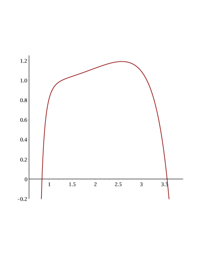
(a) $\theta=5.4$

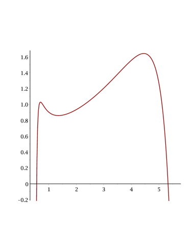
(b) $\theta=6.9$

Figure 4. The graph of the function $v\mapsto K_{1}(v;\theta)$ (i.e., with $m=1$) for $k=2$, $q=5$ and various values of $\theta>\theta_{1}=1+2\mbox{$\;\!$}\sqrt{3}\doteq 4.4641$, illustrating different possible numbers of solutions $\nu_{1}=\nu_{1}(\theta,\alpha)$ of the equation (5.25): (a)  $\theta=5.4$,  $0\leq\nu_{1}\leq 2$; (b)  $\theta=6.9$,  $0\leq\nu_{1}\leq 4$.

(a) $\theta=3.4$

(b) $\theta=4.1$

Figure 5. The graph of the function $v\mapsto K_{1}(v;\theta)$ for $q=3$ and $k=2$, illustrating the location of its maximum point depending on whether $\theta_{\rm c}<\theta<\tilde{\theta}_{1}$ or $\theta>\tilde{\theta}_{1}$; here, $\theta_{\rm c}=3$ and $\tilde{\theta}_{1}=\frac{1}{2}\bigl{(}1+\sqrt{41}\mbox{$\>\!$}\bigr{)}\doteq 3.7016$.

As mentioned in Remark 2.10, the case $q=3$ is truly critical with regard to the uniqueness. Recall that $\nu(\theta,\alpha)$ denotes the number of positive solutions of the system (2.31); the function $\alpha_{1}(\theta)$ is defined in (2.46) and $\theta_{1}^{0}$ is its zero. The proof of the next proposition relies on some lemmas that will be proved later, in Sections 6.2 and 6.3.

Proposition 5.4.

Let $q=3$ and $k\geq 2$. There exists $\varepsilon>0$ small enough such that

• $\nu(\theta,\alpha_{1}(\theta))=1$ if $1\leq\theta<\theta_{1}+\varepsilon$,

• $\nu(\theta,\alpha_{1}(\theta))\geq 2$ for all $\theta>\theta^{0}_{1}-\varepsilon$.

Proof.

(a) As shown in the proof of Lemma 5.3 (see Appendix B), $\partial^{2}K_{1}/\partial v^{2}|_{v=1}\mbox{$\;\!\!$}<0$ for all $\theta\in[\mbox{$\>\!$}\theta_{1},\tilde{\theta}_{1})$; in particular, $\partial^{2}K_{1}(\theta_{1},v)/\partial v^{2}|_{v=1}\mbox{$\;\!\!$}<0$. By Lemma 5.2(c), the set $\mathscr{V}_{1}^{+}(\theta)$ (see (2.45)) is reduced for $\theta=\theta_{1}$ to the single point $v=1$, and $K_{1}^{*}(\theta_{1})=\max_{v\in\mathscr{V}^{+}_{1}(\theta_{1})}K_{1}(v;\theta_{1})=K_{1}(1;\theta_{1})=0$. By continuity, it follows that $\partial^{2}K_{1}(\theta;v)/\partial v^{2}<0$ for each $\theta\in[\mbox{$\>\!$}\theta_{1},\theta_{1}+\varepsilon)$ and all $v\in\mathscr{V}^{+}_{1}(\theta)$; that is, the function $v\mapsto K_{1}(v;\theta)$ is concave on $\mathscr{V}^{+}_{1}(\theta)$ and therefore has a unique maximum located at $v=1$ (remembering that $\partial K_{1}/\partial v|_{v=1}\mbox{$\;\!\!$}=0$). But the solution $(u,v)$ with $v=1$ is not admissible (see (2.34)), hence $\nu(\theta,\alpha_{1}(\theta))=1$, with the only solution of (2.31) coming from equation (2.32).

(b) We have $\alpha_{1}(\theta_{1}^{0})=0$, hence $K_{1}^{*}(\theta_{1}^{0})=1$ (see (2.46)) and, by Lemma 6.15(b), also $L_{1}^{*}(\theta^{0}_{1})=1$. If $v_{1}=v_{1}(\theta_{1}^{0})$ is the point where the latter maximum is attained, that is, $L_{1}(v_{1};\theta_{1}^{0})=L_{1}^{*}(\theta_{1}^{0})=1$, then it holds that $v_{1}>1$ (see Lemma 6.7 below). Furthermore, according to Lemma 5.2(a), $v_{1}$ is the unique maximum of the function $v\mapsto L_{1}(v;\theta_{1}^{0})$, and in particular $L_{1}(1;\theta_{1}^{0})<L_{1}^{*}(\theta_{1}^{0})=1$.

From the definition (5.26), it follows that also $K_{1}(v_{1};\theta_{1}^{0})=1=K_{1}^{*}(\theta_{1}^{0})$, and since $L_{1}(1;\theta_{1}^{0})<1$, Lemma 6.15(a) implies that $K_{1}(1;\theta_{1}^{0})<1=K_{1}^{*}(\theta_{1}^{0})$. Thus, the corresponding solution of the system (2.33) satisfies the condition (2.34), and therefore $\nu(\theta_{1}^{0},\alpha_{1}(\theta_{1}^{0}))\geq 2$.

By continuity of $K_{1}(1;\theta)$ and $K_{1}^{*}(\theta)$, for all $\theta\in(\theta_{1}^{0}-\varepsilon,\theta_{1}^{0}\mbox{$\>\!$}]$ (with $\varepsilon>0$ small enough) we still have that $K_{1}(1;\theta)<K_{1}^{*}(\theta)$, so the maximum is attained outside $v=1$. Thus, by the same argument as before, the claim follows. ∎

5.5. Proof of Theorem 2.11

(a) First, let $q=2$. According to Lemma 5.1, the system (2.31) is reduced to the single equation (2.32), and by Theorem 2.8 the number of its solutions is not more than $3=2^{2}-1$; furthermore, for $\theta>\theta_{\rm c}=\frac{k+1}{k-1}$ and $\alpha_{-}(\theta)<\alpha<\alpha_{+}(\theta)$, there are exactly three solutions, so the upper bound is attained.

(b) Let now $\alpha=0$ (and $q\geq 3$). Due to Lemma 5.1(b), either $z_{i}\equiv 1$ or the system (2.32) is reduced to the equation (5.3) indexed by $m=1,\dots,q-1$, which can be rewritten as $L_{m}(u;\theta)=1$ (see (5.13)). By Lemma 5.2(a), the latter equation has no more than two roots. Hence, considering permutations of the values $u\neq 1$ over the $q-1$ places, it is clear that the total number of solutions to (2.32) is bounded by

$$1+2\sum_{m=1}^{q-1}\binom{q-1}{m}=1+2\mbox{$\;\!$}(2^{q-1}-1)=2^{q}-1.$$ (5.27)

Moreover, for $\theta>1$ large enough, there will be exactly two roots of each of the equations $L_{m}(u;\theta)=1$, because $L_{m}^{*}(\theta)=\max_{u>0}L_{m}(u;\theta)\to\infty$ as $\theta\to\infty$ (see Lemma 5.2(b)). Therefore, the upper bound (5.27) is attained.

(c) Finally, let $k=2$ and $\alpha\neq 0$. First of all, up to three solutions of the system (2.32) arising from the equation (5.4) are ensured by Lemma 5.1 (see also Theorem 2.8). Other solutions are determined by the system (5.5) indexed by $m=1,\dots,q-2$, which in turn depends on the solvability of the equation (5.25). In the case $k=2$, the latter is a polynomial equation of degree $4$, and therefore has at most four roots $v>0$, for each $m$. The value $u>0$ is then determined uniquely by formula (5.24), and it occupies the first place in the vector $\boldsymbol{z}=(z_{1},\dots,z_{q-1})$. As for the root $v>0$, it occupies $m$ out of the $q-2$ remaining places. Counting the total number of such permutations, we get the upper bound

$$3+4\sum_{m=1}^{q-2}\binom{q-1}{m}=3+4\mbox{$\;\!$}(2^{q-2}-1)=2^{q}-1,$$

as required. This completes the proof of Theorem 2.11.

6. Further properties of the critical curves $\alpha_{\pm}(\theta)$ and $\alpha_{m}(\theta)$

6.1. Properties of $\alpha_{\pm}(\theta)$

Lemma 6.1.

The quantities $a_{\pm}$, defined in (2.40) for $b\geq\left(\frac{k+1}{k-1}\right)^{2}$, satisfy the identity

$$a_{+}\times a_{-}=b^{-k-1}.$$ (6.1)

Proof.

Using (2.40) and noting that $x_{-}=b/x_{+}$ (see equation (2.37)), we find

$$a_{-} =\frac{1}{x_{-}}\left(\frac{1+x_{-}}{b+x_{-}}\right)^{k}$$

$$=\frac{x_{+}}{b}\left(\frac{1+b/x_{+}}{b+b/x_{+}}\right)^{k}$$

$$=\frac{x_{+}}{b^{k+1}}\left(\frac{b+x_{+}}{1+x_{+}}\right)^{k}$$

$$=\frac{b^{-k-1}}{a_{+}},$$

and formula (6.1) follows. ∎

Lemma 6.2.

Suppose that $b\geq\left(\frac{k+1}{k-1}\right)^{2}$. Then the following inequalities hold,

$$a_{+}<b^{-1},\qquad a_{-}>b^{-k}.$$ (6.2)

Proof.

From (5.11), for all $x\geq 0$ we get the upper bound

$$f^{\prime}(x) =\left(1+\frac{b-1}{1+x}\right)^{-k}\frac{k\mbox{$\>\!$}(b-1)}{(b+x)(1+x)}<\frac{1}{b+x}\leq\frac{1}{b},$$

noting that, by Bernoulli’s inequality,

$$\left(1+\frac{b-1}{1+x}\right)^{k}>\frac{k\mbox{$\>\!$}(b-1)}{1+x}.$$

Hence, $a_{+}=f^{\prime}(x_{+})<b^{-1}$, and the first inequality in (6.2) is proved. The second inequality then readily follows from the identity (6.1). ∎

Lemma 6.3.

The functions $\alpha_{\pm}(\theta)$ satisfy the following identity,

$$\alpha_{-}(\theta)+\alpha_{+}(\theta)=\frac{2\mbox{$\>\!$}\ln\mbox{$\>\!$}\mbox{$\>\!\!$}(q-1)+(k+1)\bigl{(}\ln b(\theta)-2\bigr{)}}{\ln\theta},\qquad\theta\geq\theta_{\rm c},$$ (6.3)

where $b(\theta)$ is defined in (2.36). In particular, if $q=2$ then $\alpha_{-}(\theta)+\alpha_{+}(\theta)\equiv 0$ for all $\theta\geq\theta_{\rm c}=\frac{k+1}{k-1}$.

Proof.

Using (5.12), we obtain

$$\theta^{\mbox{$\>\!$}2\mbox{$\>\!$}(k+1)+\alpha_{-}(\theta)+\alpha_{+}(\theta)}=\frac{(q-1)^{2}}{a_{-}(\theta)\mbox{$\;\!$}a_{+}(\theta)},\qquad\theta\geq\theta_{\rm c},$$

and the identity (6.3) follows upon substituting formula (6.1). ∎

Proposition 6.4.

The functions $\alpha_{\pm}(\theta)\colon[\theta_{\rm c},\infty)\to\mathbb{R}$ defined in (2.41) have the following “boundary” values,

$$\alpha_{\pm}(\theta_{\rm c}) =-(k+1)+\frac{1}{\ln\theta_{\rm c}}\left(\ln\mbox{$\>\!$}\mbox{$\>\!\!$}(q-1)+(k+1)\ln\frac{k+1}{k-1}\right),$$ (6.4)

$$\alpha_{\pm}(\theta) \to\pm(k-1)\qquad(\theta\to\infty).$$ (6.5)

In particular, $\alpha_{\pm}(\theta_{\rm c})=0$ if $q=2$ and $\alpha_{\pm}(\theta_{\rm c})>0$ if $q>2$.

Proof.

Recall from the proof of Theorem 2.8 (see Section 5.2) that the critical value $\theta=\theta_{\rm c}$ corresponds to $b(\theta_{\rm c})=\bigl{(}\frac{k+1}{k-1}\bigr{)}^{2}$, whereby the quadratic equation (2.37) has the double root

$$x_{\pm}(\theta_{\rm c})=\sqrt{b(\theta_{\rm c})}=\frac{k+1}{k-1}.$$

Hence, using (2.40), we find

$$a_{\pm}(\theta_{\rm c})=\left(\frac{k-1}{k+1}\right)^{k+1},$$

which, together with (5.12), yields formula (6.4).

If $q=2$ then formula (2.35) gives $\theta_{\rm c}=\frac{k+1}{k-1}$, and it readily follows from (6.4) that $\alpha(\theta_{\rm c})=0$. For $q>2$, using the relation (5.12) observe that the required inequality $\alpha_{\pm}(\theta_{\rm c})>0$ is reduced to

$$\theta_{\rm c}^{k+1}<\frac{q-1}{a_{\pm}(\theta_{\rm c})}=\left(\frac{k+1}{k-1}\right)^{k+1}(q-1),$$

that is,

$$\theta_{\rm c}<\left(\frac{k+1}{k-1}\right)(q-1)^{1/(k+1)}.$$ (6.6)

Denote

$$\rho_{k}:=\frac{k+1}{k-1}>1,\qquad s:=(q-1)^{1/(k+1)}>1,$$

then (6.6) takes the form

$$\theta_{\rm c}<\rho_{k}\mbox{$\>\!$}s.$$ (6.7)

Furthermore, recalling that $b(\theta_{\rm c})=\left(\frac{k+1}{k-1}\right)^{2}=\rho_{k}^{2}$ and $b(\theta)$ is monotone increasing for $\theta>1$ (see (2.35) and (2.36)), the inequality (6.7) is equivalent to

$$\rho_{k}^{2}=b(\theta_{\rm c})<b(\rho_{k}\mbox{$\>\!$}s)=\frac{\rho_{k}\mbox{$\>\!$}s\bigl{(}\rho_{k}\mbox{$\>\!$}s+s^{k+1}-1\bigr{)}}{s^{k+1}},$$

that is,

$$s^{k+1}-1>\rho_{k}\mbox{$\>\!$}(s^{k}-s),$$

which is reduced, upon dividing by $s-1>0$ and substituting $\rho_{k}-1=\frac{2}{k-1}$, to

$$\phi_{k}(s):=s^{k}+1-\frac{2\mbox{$\;\!$}p_{k}(s)}{k-1}>0.$$ (6.8)

In fact, it is easy to show that $\phi_{k}(s)>0$ for any $s>1$. Indeed, since $p_{k}(1)=k-1$, we have $\phi_{k}(1)=0$, while

$$\phi_{k}^{\prime}(s) =k\mbox{$\>\!$}s^{k-1}-\frac{2}{k-1}\sum_{i=1}^{k-1}i\mbox{$\>\!$}s^{i-1}$$

$$=s^{k-1}\left(k-\frac{2}{k-1}\sum_{i=1}^{k-1}i\mbox{$\>\!$}s^{-(k-i)}\right)$$

$$>s^{k-1}\left(k-\frac{2}{k-1}\sum_{i=1}^{k-1}i\right)$$

$$=s^{k-1}\left(k-\frac{2}{k-1}\cdot\frac{k\mbox{$\;\!$}(k-1}{2}\right)=0.$$

Thus, inequality (6.8) is verified, which implies that $\alpha(\theta_{\rm c})>0$, as argued above.

Let us now prove (6.5). Using the definition of $b=b(\theta)$ and $D=D(\theta)$ (see (2.36) and (2.38), respectively), we obtain the following asymptotics as $\theta\to\infty$,

$$b=\frac{\theta^{2}}{q-1}+O(\theta),\qquad\sqrt{D}=\frac{\theta^{2}(k-1)}{q-1}+O(\theta),$$

and

$$x_{+}=\frac{\theta^{2}(k-1)}{q-1}+O(\theta),\qquad x_{-}=\frac{b}{x_{+}}=\frac{1}{k-1}+O(\theta^{-1}).$$

Hence,

$$\ln x_{\pm}=(1\pm 1)\ln\theta+O(1),\qquad\ln\frac{b+x_{\pm}}{1+x_{\pm}}=(1\mp 1)\ln\theta+O(1).$$

Using formula (2.40), this yields

$$-\ln a_{\pm}(\theta) =\ln x_{\pm}+k\ln\frac{b+x_{\pm}}{1+x_{\pm}}$$

$$=\bigl{(}(k+1)\mp(k-1)\bigr{)}\ln\theta+O(1).$$

Therefore, from (5.12) we get

$$k+1+\alpha_{\pm}=-\frac{\ln a_{\mp}(\theta)}{\ln\theta}+o(1)=(k+1)\pm(k-1)+o(1),$$

and the limit (6.5) follows. ∎

Proposition 6.5.

The functions $\alpha_{\pm}(\theta)$ satisfy the following bounds,

$$\alpha_{-}(\theta) >-(k-1),\qquad \theta \geq\theta_{\rm c},$$ (6.9)

$$\alpha_{+}(\theta) <k-1,\qquad \theta \geq\max\{\theta_{\rm c},\bar{\theta}\mbox{$\>\!$}\},$$ (6.10)

where

$$\bar{\theta}=\bar{\theta}(k,q):=\begin{cases}\displaystyle\frac{q-2}{(q-1)^{(k-1)/k}-1},\quad&q>2,\\[7.20007pt] \ 1,&q=2.\end{cases}$$ (6.11)

Proof.

Using the relation (5.12), the first inequality in (6.2) and the definition of $b$ in (5.10), we get

$$\theta^{\mbox{$\>\!$}k+1+\alpha_{-}}=\frac{q-1}{a_{+}} >(q-1)\mbox{$\;\!$}b$$

$$=\theta\mbox{$\>\!$}(\theta+q-2)\geq\theta^{2},\qquad q\geq 2,$$

which proves the bound (6.9).

Similarly, using the second inequality in (6.2) we have

$$\theta^{\mbox{$\>\!$}k+1+\alpha_{+}}=\frac{q-1}{a_{-}} <(q-1)\mbox{$\;\!$}b^{k}$$

$$=(q-1)^{1-k}\mbox{$\;\!$}\theta^{2k}\!\left(1+\frac{q-2}{\theta}\right)^{k}.$$ (6.12)

Noting from (6.11) that, for $\theta\geq\bar{\theta}$,

$$1+\frac{q-2}{\theta}\leq 1+\frac{q-2}{\bar{\theta}}=(q-1)^{(k-1)/k},\qquad q\geq 2,$$

it is easy to see that the right-hand side of (6.12) is bounded above by $\theta^{2k}$; hence, the inequality (6.10) follows. ∎

Remark 6.1.

Note that $\bar{\theta}>1$ for $q\geq 3$. Of course, if $\theta_{\rm c}\geq\bar{\theta}$ then the upper bound (6.10) holds for all $\theta\geq\theta_{\rm c}$; however, the ordering between $\theta_{\rm c}$ and $\bar{\theta}$ depends on $k$ and $q$. For example, for $k=2$ and $q=5$

$$\bar{\theta}=3<\theta_{\rm c}\doteq 4.6847,$$

whereas for $k=2$ and $q=50$

$$\bar{\theta}=8>\theta_{\rm c}\doteq 7.8904.$$

In fact, for large $q$ the upper bound (6.10) fails near $\theta_{\rm c}$; indeed, using (2.35) we get

$$\theta_{\rm c}=\frac{q-2}{2}\left(\sqrt{1+\frac{4\mbox{$\>\!$}(q-1)}{(q-2)^{2}}\left(\frac{k+1}{k-1}\right)^{2}}-1\right)\sim\left(\frac{k+1}{k-1}\right)^{2},\qquad q\to\infty,$$

and, according to (6.4),

$$\alpha_{\pm}(\theta_{\rm c})\sim\frac{\ln q}{\ln\theta_{\rm c}}\to\infty,\qquad q\to\infty.$$

Conjecture 6.1.

The function $\alpha_{-}(\theta)$ is monotone decreasing for all $\theta\geq\theta_{\rm c}$, whereas $\alpha_{+}(\theta)$ is decreasing for $\theta\leq\theta^{+}_{0}$ and increasing for $\theta\geq\theta^{+}_{0}$, with the unique minimum $\alpha_{+}(\theta^{+}_{0})=0$ at the critical point

$$\theta^{+}_{0}=\theta^{+}_{0}(k,q):=1+\frac{q}{k-1}.$$ (6.13)

In the case $q=2$, we have $\theta_{\rm c}=\theta_{0}^{+}=\frac{k+1}{k-1}$ and, by Lemma 6.3, $\alpha_{+}(\theta)\equiv-\alpha_{-}(\theta)$; hence, the function $\alpha_{+}(\theta)$ should be monotone increasing for all $\theta\geq\theta_{\rm c}$.

This conjecture is supported by computer plots (see Figure 6). Towards a proof, we have been able to characterize the unique zero $\theta_{0}^{-}$ of $\alpha_{-}(\theta)$ and to show rigorously that $\alpha_{+}(\theta^{+}_{0})=0$ and $\alpha^{\prime}_{+}(\theta^{+}_{0})=0$ (see Proposition 6.16(b)), but the monotonicity properties are more cumbersome to verify.

Remark 6.2.

Note that the value (6.13) coincides with a known critical point in the case $\alpha=0$, above which the solution $\boldsymbol{z}=\boldsymbol{1}$ is unstable (see [47, Section 5.2.2.2, Proposition 5.4]). Our Proposition 6.16(b-i) explains the emergence of this critical point and its explicit value (6.13).

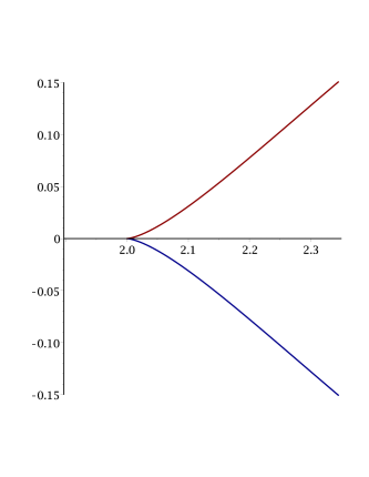
(a) $q=2$ ($k=3$)

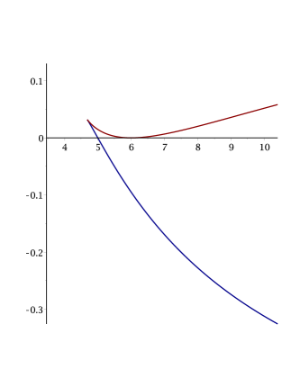
(b) $q=5$ ($k=2$)

Figure 6. The graphs of the functions $\alpha_{+}(\theta)$ and $\alpha_{-}(\theta)$ (see (2.41)): (a) $q=2$, $k=3$; (b) $q=5$, $k=2$. The coordinates of the cusp point $C$ (see (2.35) and (6.4)) are given numerically by: (a) $\theta_{\rm c}=2$, $\alpha_{\pm}(\theta_{\rm c})=0$; (b) $\theta_{\rm c}\doteq 4.6847$, $\alpha_{\pm}(\theta_{\rm c})\doteq 0.0319$. The axis $\alpha=0$ is a tangent line for $\alpha_{+}(\theta)$ at $\theta^{+}_{0}\!=1+q/(k-1)$ (see Proposition 6.16(b-i)): (a) $\theta^{+}_{0}\!=2\;({=}\>\theta_{\rm c})$; (b) $\theta^{+}_{0}\!=6$. In panel (b), the function $\alpha_{-}(\theta)$ has zero at $\theta^{-}_{0}\!=5$ (see Proposition 6.16(b-ii) and Example 6.1), whereas in panel (a) we have $\theta_{0}^{-}\!=\theta_{0}^{+}\!=2$ (see Proposition 6.4). Note that the graphs display the monotone behaviour as predicted by Conjecture 6.1.

6.2. Properties of $L_{m}(v;\theta)$ and $K_{m}(v;\theta)$

Here and below, we assume that $q\geq 3$. Recall that $v_{m}=v_{m}(\theta)$ is the unique maximum of the function $v\mapsto L_{m}(v;\theta)$ (see Lemma 5.2(a)), and $\theta_{m}$ is defined by the relation (5.15), where $1\leq m\leq q-2$.

Remark 6.3.

All results in this section hold true for a continuous parameter $m$ (cf. Remark 5.2), which is evident by inspection of the proofs.

The next lemma describes the useful scaling properties of the functions $L_{m}(v;\theta)$ and $K_{m}(v;\theta)$ (see (5.13) and (5.26)) under the conjugation $m\mapsto m^{\prime}$.

Lemma 6.6.

For each $m=1,\dots,q-2$ and $m^{\prime}=q-1-m$, the following identities hold for all $v>0$ and $\theta>\theta_{m}$,

$$L_{m^{\prime}}(v;\theta) =v^{k}L_{m}(v^{-1};\theta),$$ (6.14)

$$K_{m^{\prime}}(v;\theta) =K_{m}(v^{-1};\theta).$$ (6.15)

Proof.

Recalling the notation (5.1), note that

$$p_{k}(v^{-1})=v^{-(k-1)}+\dots+v^{-1}=v^{-k}p_{k}(v),$$ (6.16)

and similarly

$$p_{k}(v^{-1})+1=v^{-(k-1)}+\dots+v^{-1}+1=v^{-k+1}\bigl{(}p_{k}(v)+1\bigr{)}.$$ (6.17)

Using (5.13) and (6.16), we can write

$$L_{m}(v^{-1};\theta) =(\theta-1)\mbox{$\;\!$}p_{k}(v^{-1})-mv^{-k}-m^{\prime}$$

$$=v^{-k}\left((\theta-1)\mbox{$\;\!$}p_{k}(v)-m-m^{\prime}v^{k}\right)$$

$$=v^{-k}L_{m^{\prime}}(v;\theta),$$

and formula (6.14) follows. Furthermore, using (6.14) and substituting (6.16) and (6.17), we obtain

$$K_{m}(v^{-1};\theta) =\frac{L_{m}(v^{-1};\theta)\bigl{(}p_{k}(v^{-1})+1\bigr{)}^{k}}{\bigl{(}p_{k}(v^{-1})+L_{m}(v^{-1};\theta)\bigr{)}^{k}}$$

$$=\frac{v^{-k}L_{m^{\prime}}(v;\theta)\cdot v^{-(k-1)\mbox{$\>\!$}k}\bigl{(}p_{k}(v)+1\bigr{)}^{k}}{\bigl{(}v^{-k}p_{k}(v)+v^{-k}L_{m^{\prime}}(v;\theta)\bigr{)}^{k}}$$

$$=\frac{L_{m^{\prime}}(v;\theta)\bigl{(}p_{k}(v)+1\bigr{)}^{k}}{\bigl{(}p_{k}(v)+L_{m^{\prime}}(v;\theta)\bigr{)}^{k}}$$

$$=K_{m^{\prime}}(v;\theta),$$

which proves formula (6.15). ∎

For $\theta>\theta_{m}$, let $v_{m}=v_{m}(\theta)$ be the point where the function $v\mapsto L_{m}(v;\theta)$ attains its (positive) maximum value, that is, $L_{m}(v_{m};\theta)=\max_{v\in\mathscr{V}_{m}^{+}(\theta)}L_{m}(v;\theta)$ (see Lemma 5.2). The next result provides a strict lower bound for $v_{m}$ (cf. Lemma 5.2(c) for $\theta=\theta_{m}$).

Lemma 6.7.

For all $m$ in the range $1\leq m\leq\frac{1}{2}\mbox{$\>\!$}(q-1)$, we have

$$v_{m}(\theta)>1,\qquad\theta>\theta_{m}.$$ (6.18)

Proof.

To the contrary, suppose first that $v_{m}<1$ for some $\theta>\theta_{m}$. Then, according to Lemma 6.6, we have

$$L_{m}(v_{m}^{-1};\theta)=v_{m}^{-k}L_{m^{\prime}}(v_{m};\theta)>L_{m^{\prime}}(v_{m};\theta),$$ (6.19)

and furthermore,

$$L_{m^{\prime}}(v_{m};\theta) =(\theta-1)\mbox{$\;\!$}p_{k}(v_{m})-m^{\prime}v_{m}^{k}-m$$

$$=L_{m}(v_{m};\theta)+(m^{\prime}-m)(1-v_{m}^{k})\geq L_{m}(v_{m};\theta),$$ (6.20)

since $m^{\prime}=q-1-m\geq m$ by the hypothesis of the lemma. Combining (6.19) and (6.20), we see that $L_{m}(v_{m}^{-1};\theta)>L_{m}(v_{m};\theta)$, which contradicts the assumption that $L_{m}(v_{m};\theta)$ is the maximum value of the function $v\mapsto L_{m}(v;\theta)$.

Assume now that $v_{m}=1$ for some $\theta>\theta_{m}$. Then

$$\left.\frac{\partial L(v;\theta)}{\partial v}\right|_{v=v_{m}=1}\!=(\theta-1)\mbox{$\;\!$}p^{\prime}_{k}(1)-k\mbox{$\>\!$}m=(\theta-1)\mbox{$\;\!$}\frac{k\mbox{$\>\!$}(k-1)}{2}-k\mbox{$\>\!$}m=0,$$

whence $(\theta-1)(k-1)=2\mbox{$\>\!$}m$. Hence,

$$L_{m}(1;\theta)=(\theta-1)(k-1)-(q-1)=2\mbox{$\>\!$}m-(q-1)\leq 0,$$

which contradicts the assumption $L_{m}(v_{m};\theta)>0$.

Thus, the inequality (6.18) is proved. ∎

For $\theta>\theta_{m}$, let $w_{m}=w_{m}(\theta)$ be the point where the function $v\mapsto K_{m}(v;\theta)$ attains its (positive) maximum value, that is, $K_{m}(w_{m};\theta)=\max_{v\in\mathscr{V}_{m}^{+}(\theta)}K_{m}(v;\theta)$. Note that $w_{m}(\theta_{m})=v_{m}(\theta_{m})=v_{m}^{*}$ (see Lemma 5.2(c)). The importance of the next technical lemma is pinpointed by involvement of the expression $p_{k}(v)-(k-1)\mbox{$\;\!$}L_{m}(v;\theta)$ in the partial derivative $\partial K_{m}/\partial v$ (see formula (6.23) below).

Lemma 6.8.

Let $1\leq m\leq\frac{1}{2}\mbox{$\>\!$}(q-1)$ and $\theta>\theta_{m}$.

• Let $w\in\mathscr{V}_{m}^{+}(\theta)$ be a critical point of the function $v\mapsto K_{m}(v;\theta)$, that is, any solution of the equation $\partial K_{m}/\partial v=0$. Assume that either (i) $w<v_{m}$ and $L_{m}(w;\theta)<1$, or (ii) $w\geq v_{m}$. Then

  $$p_{k}(w)-(k-1)\mbox{$\;\!$}L_{m}(w;\theta)>0.$$ (6.21)

• In particular, the inequality (6.21) holds for $w=w_{m}$, that is,

  $$p_{k}(w_{m})-(k-1)\mbox{$\;\!$}L_{m}(w_{m};\theta)>0.$$ (6.22)

Proof.

(a) From the definition (5.26), compute the partial derivative

$$\frac{\partial K_{m}}{\partial v}=\frac{(p_{k}+1)^{k-1}}{(p_{k}+L_{m})^{k+1}}\left((p_{k}+1)\bigl{(}p_{k}-(k-1)\mbox{$\>\!$}L_{m}\bigr{)}\mbox{$\>\!$}\frac{\partial L_{m}}{\partial v}-k\mbox{$\>\!$}L_{m}(1-L_{m})\mbox{$\;\!$}p^{\prime}_{k}\right),$$ (6.23)

with the shorthand notation $p_{k}:=p_{k}(v)$ and $L_{m}:=L_{m}(v;\theta)$. Hence, the condition $\partial K_{m}/\partial v=0$ is reduced to the equality

$$(p_{k}+1)\bigl{(}p_{k}-(k-1)\mbox{$\>\!$}L_{m}\bigr{)}\mbox{$\>\!$}\frac{\partial L_{m}}{\partial v}-k\mbox{$\>\!$}L_{m}(1-L_{m})\mbox{$\;\!$}p^{\prime}_{k}=0.$$ (6.24)

If $w<v_{m}$ then $\partial L_{m}/\partial v|_{v=w}\mbox{$\;\!\!$}>0$, and the required inequality (6.21) readily follows from equation (6.24) using that $L_{m}(w;\theta)<1$. Similarly, if $w>v_{m}$ then $\partial L_{m}/\partial v|_{v=w}\mbox{$\;\!\!$}<0$ and equation (6.24) implies the inequality (6.21) provided that $L_{m}(w;\theta)>1$. Alternatively, if $L_{m}(w;\theta)\leq 1$ then, noting that $w>v_{m}>1$ (by Lemma 6.7), we obtain, in agreement with (6.21),

$$p_{k}(w)>p_{k}(1)=k-1\geq(k-1)\mbox{$\;\!$}L_{m}(w;\theta),$$ (6.25)

because the function $w\mapsto p_{k}(w)$ is strictly increasing and $p_{k}(1)=k-1$.

Lastly, if $w=v_{m}$ then $\partial L_{m}/\partial v|_{v=v_{m}}\mbox{$\;\!\!$}=0$ and equation (6.24) implies $L_{m}(v_{m};\theta)=1$. Again using Lemma 6.7, similarly to (6.25) we get

$$p_{k}(w)=p_{k}(v_{m})>p_{k}(1)=k-1=(k-1)\mbox{$\;\!$}L_{m}(w;\theta),$$ (6.26)

so the inequality (6.21) holds in this case as well.

(b) Let $w=w_{m}$ be the point of maximum of the function $v\mapsto K_{m}(v;\theta)$. According to part (a), we only have to consider the case where $w_{m}<v_{m}$ and $L_{m}(w_{m};\theta)\geq 1$.

If $L_{m}(w_{m};\theta)>1$, let $\kern 0.6458pt\hbox{\vbox{\hrule height=0.4pt\kern 1.29167pt\hbox{\kern-1.49994pt$w$\kern-1.00006pt}}\kern 1.07639pt}>v_{m}>w_{m}$ be such that $L_{m}(\kern 0.6458pt\hbox{\vbox{\hrule height=0.4pt\kern 1.29167pt\hbox{\kern-1.49994pt$w$\kern-1.00006pt}}\kern 1.07639pt};\theta)=L_{m}(w_{m};\theta)$, then

$$K_{m}(\kern 0.6458pt\hbox{\vbox{\hrule height=0.4pt\kern 1.29167pt\hbox{\kern-1.49994pt$w$\kern-1.00006pt}}\kern 1.07639pt};\theta) =L_{m}(\kern 0.6458pt\hbox{\vbox{\hrule height=0.4pt\kern 1.29167pt\hbox{\kern-1.49994pt$w$\kern-1.00006pt}}\kern 1.07639pt};\theta)\left(1-\frac{L_{m}(\kern 0.6458pt\hbox{\vbox{\hrule height=0.4pt\kern 1.29167pt\hbox{\kern-1.49994pt$w$\kern-1.00006pt}}\kern 1.07639pt};\theta)-1}{p_{k}(\kern 0.6458pt\hbox{\vbox{\hrule height=0.4pt\kern 1.29167pt\hbox{\kern-1.49994pt$w$\kern-1.00006pt}}\kern 1.07639pt})+L_{m}(\kern 0.6458pt\hbox{\vbox{\hrule height=0.4pt\kern 1.29167pt\hbox{\kern-1.49994pt$w$\kern-1.00006pt}}\kern 1.07639pt};\theta)}\right)^{k}$$

$$=L_{m}(w_{m};\theta)\left(1-\frac{L_{m}(w_{m};\theta)-1}{p_{k}(\kern 0.6458pt\hbox{\vbox{\hrule height=0.4pt\kern 1.29167pt\hbox{\kern-1.49994pt$w$\kern-1.00006pt}}\kern 1.07639pt})+L_{m}(w_{m};\theta)}\right)^{k}$$

$$>L_{m}(w_{m};\theta)\left(1-\frac{L_{m}(w_{m};\theta)-1}{p_{k}(w_{m})+L_{m}(w_{m};\theta)}\right)^{k}$$

$$=K_{m}(w_{m};\theta).$$ (6.27)

Thus, $K_{m}(\kern 0.6458pt\hbox{\vbox{\hrule height=0.4pt\kern 1.29167pt\hbox{\kern-1.49994pt$w$\kern-1.00006pt}}\kern 1.07639pt};\theta)>K_{m}(w_{m};\theta)$, which contradicts the assumption that $v=w_{m}$ provides the maximum value of the function $v\mapsto K_{m}(v;\theta)$.

Lastly, suppose that, for some $\theta>\theta_{m}$,

$$L_{m}(w_{m};\theta)=1.$$ (6.28)

In view of the definition (5.26), condition (6.28) implies that $K_{m}(w_{m};\theta)=1$. Let us prove that in this case we must have $w_{m}>1$, which would then automatically imply the required inequality (6.22) (cf. (6.25) and (6.26)). To the contrary, assume that $w_{m}\leq 1$. If $w_{m}=1$ then, using the definition (5.13) and recalling that $m+m^{\prime}=q-1$, the equation (6.28) is reduced to

$$L_{m}(1;\theta)=(\theta-1)(k-1)-(q-1)=1,$$

whence we find

$$\theta=1+\frac{q}{k-1}.$$ (6.29)

Furthermore, noting that

$$p_{k}^{\prime}(1)=\sum_{i=1}^{k-1}i=\frac{k\mbox{$\>\!$}(k-1)}{2}$$ (6.30)

and substituting (6.29), from (5.13) we get

$$\frac{\partial L_{m}(1;\theta)}{\partial v}=(\theta-1)\mbox{$\;\!$}\frac{k\mbox{$\>\!$}(k-1)}{2}-k\mbox{$\>\!$}m=k\left(\frac{q}{2}-m\right)>0,$$

since $m\leq\frac{1}{2}(q-1)<q/2$. Thus, $w_{m}=1$ is the left root of the equation $L_{m}(v;\theta)=1$. Denote by $\bar{v}>1$ the right root, that is, $L_{m}(\bar{v};\theta)=1$ and $\partial L_{m}/\partial v|_{v=\bar{v}}\mbox{$\;\!\!$}<0$. It follows that $K_{m}(\bar{v};\theta)=1$ (see (5.26)), so the maximum value $1$ of the function $v\mapsto K_{m}(v;\theta)$ is also attained at $v=\bar{v}>1$. Returning to formula (6.23), observe that

$$\frac{\partial K_{m}(\bar{v};\theta)}{\partial v}=\frac{p_{k}(\bar{v})-(k-1)}{p_{k}(\bar{v})+1}\times\frac{\partial L_{m}(\bar{v};\theta)}{\partial v}<0,$$ (6.31)

because $p_{k}(\bar{v})>p_{k}(1)=k-1$ and, as mentioned above, $\partial L_{m}/\partial v|_{v=\bar{v}}\mbox{$\;\!\!$}<0$. But the inequality (6.31) implies that there are points $v<\bar{v}$ such that $K_{m}(v;\theta)>K_{m}(\bar{v};\theta)$, a contradiction. Hence, the case $w_{m}=1$ is impossible.

Now, suppose that $w_{m}<1$. Then $p_{k}(w_{m})<p_{k}(1)=k-1$ and, in view of the condition (6.28), from equation (6.24) it readily follows that $\partial L_{m}/\partial v|_{v=w_{m}}\mbox{$\;\!\!$}=0$, that is, $L_{m}(w_{m};\theta)=1$ is the maximum value of the function $v\mapsto L_{m}(v;\theta)$. Hence, for all $v<w_{m}$ we have

$$L_{m}(v;\theta)<1,\qquad\frac{\partial L_{m}(v;\theta)}{\partial v}>0.$$ (6.32)

On the other hand, by (6.24) and monotonicity of $p_{k}(v)$,

$$p_{k}(w_{m})-(k-1)\mbox{$\>\!$}L_{m}(w_{m};\theta) =p_{k}(w_{m})-(k-1)$$

$$<p_{k}(1)-(k-1)=0.$$ (6.33)

By continuity of the functions $v\mapsto p_{k}(v)$ and $v\mapsto L_{m}(v;\theta)$, the inequality (6.33) is preserved for all $v<w_{m}$ close enough to $w_{m}$:

$$p_{k}(v)-(k-1)\mbox{$\>\!$}L_{m}(v;\theta)<0.$$ (6.34)

Using (6.32) and (6.34), from (6.23) it follows that for such $v$ we have $\partial K_{m}/\partial v<0$. But this means that the function $v\mapsto K_{m}(v;\theta)$ is decreasing in the left vicinity of $w_{m}$, and thus $w_{m}$ cannot be a maximum, in contradiction with our assumption. Thus, we have proved that $w_{m}>1$ as required, which completes the proof of Lemma 6.8. ∎

The next two lemmas provide useful bounds on $w_{m}=w_{m}(\theta)$. First, there is a simple uniform upper bound.

Lemma 6.9.

For all $m\in[1,q-2\mbox{$\>\!$}]$,

$$w_{m}<\theta,\qquad\theta\geq\theta_{m}.$$ (6.35)

Proof.

Observe, using the definition (5.13), that

$$L_{m}(v;\theta)|_{v=\theta} =(\theta-1)\mbox{$\;\!$}p_{k}(\theta)-m\mbox{$\>\!$}\theta^{k}-m^{\prime}$$

$$=(\theta-1)(\theta^{k-1}+\dots+\theta)-m\mbox{$\>\!$}\theta^{k}-m^{\prime}$$

$$=-(m-1)\mbox{$\>\!$}\theta^{k}-\theta-m^{\prime}<0,$$

and also (cf. (5.17))

$$\left.\frac{\partial L_{m}(v;\theta)}{\partial v}\right|_{v=\theta} =(\theta-1)\mbox{$\;\!$}p^{\prime}_{k}(\theta)-km\mbox{$\>\!$}\theta^{k-1}$$

$$=(\theta-1)\mbox{$\;\!$}\bigl{(}(k-1)\mbox{$\>\!$}\theta^{k-2}+\dots+2\mbox{$\>\!$}\theta+1\bigr{)}-km\mbox{$\>\!$}\theta^{k-1}$$

$$=-(km-k+1)\mbox{$\>\!$}\theta^{k-1}-\theta^{k-2}-\dots-\theta-1<0.$$

Hence, the point $v=\theta$ lies to the right of the set $\mathscr{V}_{m}^{+}(\theta)=\{v>0\colon L_{m}(v;\theta)>0\}$ (see (2.45)). But $w_{m}\in\mathscr{V}_{m}^{+}(\theta)$ and therefore $w_{m}<\theta$, as claimed in (6.35). ∎

The important lower bound for $w_{m}=w_{m}(\theta)$ is established next.

Lemma 6.10.

• For all $m$ in the range $1\leq m<\frac{1}{2}(q-1)$, we have

  $$w_{m}>1,\qquad\theta>\theta_{m}.$$ (6.36)

• If $m=\frac{1}{2}\mbox{$\>\!$}(q-1)$ then the maximum point $w_{m}$ (which may not be unique) can be chosen so that $w_{m}\geq 1$.

Proof.

If $L_{m}(w_{m};\theta)\geq 1$ then, by the inequality (6.22) of Lemma 6.8,

$$p_{k}(w_{m})>(k-1)\mbox{$\>\!$}L_{m}(w_{m};\theta)\geq k-1=p_{k}(1),$$

which implies, due to the monotonicity of $p_{k}(\cdot)$, that $w_{m}>1$, in line with (6.36). Thus, it remains to consider the case $L_{m}(w_{m};\theta)<1$.

Assume first that $w_{m}=1$ for some $\theta>\theta_{m}$. Using the definition (5.13) and the value $p_{k}(1)=k-1$, we have

$$L_{m}(1;\theta) =(\theta-1)\mbox{$\;\!$}p_{k}(1)-m-m^{\prime}$$

$$=(\theta-1)(k-1)-(q-1),$$ (6.37)

and also, recalling formula (6.30),

$$\frac{\partial L_{m}(1;\theta)}{\partial v} =(\theta-1)\mbox{$\;\!$}p^{\prime}_{k}(1)-k\mbox{$\>\!$}m$$

$$=\frac{k}{2}\bigl{(}(\theta-1)(k-1)-2\mbox{$\>\!$}m\bigr{)}$$

$$=\frac{k}{2}\bigl{(}L_{m}(1;\theta)+m^{\prime}-m\bigr{)}.$$ (6.38)

Substituting (6.30), (6.37) and (6.38) into (6.23), it is easy to check that the condition $\partial K_{m}/\partial v|_{v=1}\mbox{$\;\!\!$}=0$ (see (6.24)) is reduced to

$$\bigl{(}1-L_{m}(1;\theta)\bigr{)}(m^{\prime}-m)=0.$$ (6.39)

Since $L_{m}(1;\theta)=L_{m}(w_{m};\theta)<1$ by assumption, the condition (6.39) is only satisfied if $m^{\prime}-m=0$, that is, $m=\frac{1}{2}(q-1)$. Conversely, if $m=\frac{1}{2}(q-1)$ (i.e., $m^{\prime}=m$) then, by the scaling formula (6.15) of Lemma 6.6, we have the identity

$$K_{m}(v^{-1};\theta)=K_{m^{\prime}}(v;\theta)=K_{m}(v;\theta),\qquad\theta>\theta_{m},\ v>0,$$ (6.40)

which implies that the maximum point $w_{m}=w_{m}(\theta)$ can always be chosen so as to satisfy the inequality $w_{m}\geq 1$, which proves part (b) of the lemma.

Finally, let $m<\frac{1}{2}(q-1)$ and $w_{m}<1$ for some $\theta>\theta_{m}$. Denote $L_{m}^{*}(\theta):=L_{m}(v_{m}(\theta);\theta)=\max_{v\in\mathscr{V}_{m}^{+}(\theta)}L_{m}(v;\theta)$ (see Lemma 5.2 and the definition (2.45)). We need to distinguish between two subcases, (i) $L_{m}^{*}(\theta)\leq 1$ and (ii) $L_{m}^{*}(\theta)>1$, which require a different argumentation.

(i) Assuming first that $L_{m}^{*}(\theta)\leq 1$, we will show that then

$$K_{m}(w_{m}^{-1};\theta)>K_{m}(w_{m};\theta),$$ (6.41)

which would contradict the assumption that $K_{m}(w_{m};\theta)$ is the maximum value. By formula (6.15) of Lemma 6.6, we have $K_{m}(w_{m}^{-1};\theta)=K_{m^{\prime}}(w_{m};\theta)$. Hence, recalling the definition (5.26) of the function $K_{m}(v;\theta)$, the inequality (6.41) is reduced to

$$\frac{L_{m^{\prime}}(w_{m};\theta)}{\bigl{(}p_{k}(w_{m})+L_{m^{\prime}}(w_{m};\theta)\bigr{)}^{k}}>\frac{L_{m}(w_{m};\theta)}{\bigl{(}p_{k}(w_{m})+L_{m}(w_{m};\theta)\bigr{)}^{k}}.$$ (6.42)

Note that (cf. (6.20))

$$L_{m^{\prime}}(w_{m};\theta) =(\theta-1)\mbox{$\;\!$}p_{k}(w_{m})-m^{\prime}w_{m}^{k}-m$$

$$=L_{m}(w_{m};\theta)+(m^{\prime}-m)(1-w_{m}^{k})$$

$$>L_{m}(w_{m};\theta).$$

Hence, for the proof of the inequality (6.42), it suffices to show that the function $L\mapsto L\mbox{$\>\!$}(p_{k}(w_{m})+L)^{-k}$ is strictly increasing on the interval $L\in[L_{m}(w_{m};\theta),L_{m^{\prime}}(w_{m};\theta)]$. Computing the derivative of this function, we see that the claim holds provided that

$$\frac{p_{k}(w_{m})}{k-1}>L,\qquad L_{m}(w_{m};\theta)\leq L\leq L_{m^{\prime}}(w_{m};\theta),$$

or simply if

$$\frac{p_{k}(w_{m})}{k-1}>L_{m^{\prime}}(w_{m};\theta).$$ (6.43)

The inequality (6.43) is easy to prove. Indeed, using the assumption $w_{m}<1$, observe from the definition (5.1) that

$$\frac{p_{k}(w_{m})}{k-1}>w_{m}^{k-1}>w_{m}^{k}.$$ (6.44)

On the other hand, according to the scaling formula (6.14) of Lemma 6.6, we have

$$L_{m^{\prime}}(w_{m};\theta)=w_{m}^{k}\mbox{$\;\!$}L_{m}(w_{m}^{-1};\theta)\leq w_{m}^{k}\mbox{$\;\!$}L_{m}^{*}(\theta)\leq w_{m}^{k},$$ (6.45)

by virtue of the assumption $L^{*}_{m}(\theta)\leq 1$. Now, the required inequality (6.43) readily follows from the estimates (6.44) and (6.45).

Thus, the inequality (6.41) is proved, and therefore the assumptions $w_{m}<1$ and $L_{m}^{*}(\theta)\leq 1$ are incompatible.

(ii) Assume now that $L_{m}^{*}(\theta)=L_{m}(v_{m};\theta)>1$ and, as before, $w_{m}=w_{m}(\theta)<1$. Denote

$$W_{m}=W_{m}(\theta):=\left\{w>1\colon\left.\frac{\partial K_{m}(v;\theta)}{\partial v}\right|_{v=w}\!=0\right\},$$

that is, the set of all critical points of the function $v\mapsto K_{m}(v;\theta)$ (i.e., satisfying the equation (6.24)) that lie to the right of point $v=1$. By assumption,

$$K_{m}(w_{m};\theta)>\max_{w\in W_{m}}K_{m}(w;\theta),$$ (6.46)

and our aim is to show that this leads to a contradiction.

Since $\partial L_{m}/\partial v|_{v=v_{m}}\mbox{$\;\!\!$}=0$ and $L_{m}(v_{m};\theta)>1$, formula (6.23) implies $\partial K_{m}/\partial v|_{v=v_{m}}\mbox{$\;\!\!$}>0$ and, therefore, there is at least one critical point $w>v_{m}$, which then automatically belongs to the set $W_{m}$, because $v_{m}>1$ by Lemma 6.7. There may also be critical points $w\in W_{m}$ such that $1<w<v_{m}$; for these we may assume, without loss of generality, that $L_{m}(w;\theta)<1$, for otherwise we consider the point $\kern 0.6458pt\hbox{\vbox{\hrule height=0.4pt\kern 1.29167pt\hbox{\kern-1.49994pt$w$\kern-1.00006pt}}\kern 1.07639pt}>v_{m}>w$ such that $L_{m}(\kern 0.6458pt\hbox{\vbox{\hrule height=0.4pt\kern 1.29167pt\hbox{\kern-1.49994pt$w$\kern-1.00006pt}}\kern 1.07639pt};\theta)=L_{m}(w;\theta)$, and it follows (similarly to the derivation of inequality (6.27)) that $K_{m}(\kern 0.6458pt\hbox{\vbox{\hrule height=0.4pt\kern 1.29167pt\hbox{\kern-1.49994pt$w$\kern-1.00006pt}}\kern 1.07639pt};\theta)\geq K_{m}(w;\theta)$, which means that such $w$ can be removed from the set $W_{m}$ without affecting the maximum in (6.46).

Now, the idea is to increase the index $m$. Namely, treating $m$ as a continuous parameter (see Remark 6.3), differentiate the function $m\mapsto K_{m}(w_{m}(\theta);\theta)$ to obtain

$$\frac{\partial K_{m}(w_{m};\theta)}{\partial m} =\frac{\partial K_{m}(v;\theta)}{\partial v}\biggr{|}_{v=w_{m}}\!\times\frac{\partial w_{m}(\theta)}{\partial m}$$

$$\quad+\frac{\partial K_{m}(w_{m};\theta)}{\partial L}\biggr{|}_{L=L_{m}(w_{m};\theta)}\!\times\frac{\partial L_{m}(v;\theta)}{\partial m}\biggr{|}_{v=w_{m}}$$

$$=\frac{\bigl{(}p_{k}(w_{m})+1\bigr{)}^{k}\bigl{(}p_{k}(w_{m})-(k-1)\mbox{$\>\!$}L_{m}(w_{m};\theta)\bigr{)}}{\bigl{(}p_{k}(w_{m})+L_{m}(w_{m};\theta)\bigr{)}^{k+1}}\times\bigl{(}1-w_{m}^{k}\bigr{)},$$ (6.47)

where we used the condition $\partial K_{m}/\partial v|_{v=w_{m}}\mbox{$\;\!\!$}=0$ and the definitions (5.13) and (5.26). Owing to Lemma 6.8(b), the right-hand side of (6.47) is positive and, therefore, the function $m\mapsto K_{m}(w_{m};\theta)$ is monotone increasing as long as $w_{m}<1$ and $m<m_{0}:=\frac{1}{2}\mbox{$\>\!$}(q-1)$. Likewise, every critical point $w=w^{(i)}$ from the original (finite) set $W_{m}$ generates a continuously differentiable branch $m\mapsto w_{m}^{(i)}$ as a function of the increasing variable $m$, and an argument similar to (6.47), now based on Lemma 6.8(a), yields that the corresponding function $m\mapsto\max_{w\in W_{m}}K_{m}(w;\theta)$ is monotone decreasing up to $m=m_{0}$.

If for some $\widetilde{m}\in(m,m_{0})$ it occurs that $w_{\widetilde{m}}=1$ then, by continuity, $\partial K_{\widetilde{m}}/\partial v|_{v=1}\mbox{$\;\!\!$}=0$, which implies, as was shown before (see (6.39)), that $L_{\widetilde{m}}(w_{\widetilde{m}};\theta)=1$ and therefore $K_{\widetilde{m}}(w_{\widetilde{m}};\theta)=1$ is the maximum value of the function $v\mapsto K_{\widetilde{m}}(v;\theta)$. Moreover, combining the monotonicity properties established above with the hypothetical inequality (6.46), this implies

$$1=K_{\widetilde{m}}(w_{\widetilde{m}};\theta)>K_{m}(w_{m};\theta)>\max_{w\in W_{m}}K_{m}(w;\theta)>\max_{w\in W_{\widetilde{m}}}\!K_{\widetilde{m}}(w;\theta),$$

that is,

$$\max_{w\in W_{\widetilde{m}}}\!K_{\widetilde{m}}(w;\theta)<1.$$ (6.48)

But this cannot be true, because there is $\kern 0.6458pt\hbox{\vbox{\hrule height=0.4pt\kern 1.29167pt\hbox{\kern-1.49994pt$w$\kern-1.00006pt}}\kern 1.07639pt}>v_{\widetilde{m}}$ where $L_{\widetilde{m}}(\kern 0.6458pt\hbox{\vbox{\hrule height=0.4pt\kern 1.29167pt\hbox{\kern-1.49994pt$w$\kern-1.00006pt}}\kern 1.07639pt};\theta)=1$, so that $K_{\widetilde{m}}(\kern 0.6458pt\hbox{\vbox{\hrule height=0.4pt\kern 1.29167pt\hbox{\kern-1.49994pt$w$\kern-1.00006pt}}\kern 1.07639pt};\theta)=1$ is another maximum and, hence, $\kern 0.6458pt\hbox{\vbox{\hrule height=0.4pt\kern 1.29167pt\hbox{\kern-1.49994pt$w$\kern-1.00006pt}}\kern 1.07639pt}\in W_{\widetilde{m}}$, thus contradicting (6.48).

This shows that we can exploit the monotonicity properties with respect to variable $m$ up to the final value $m=m_{0}=\frac{1}{2}(q-1)$, so that

$$K_{m}(w_{m};\theta)<K_{m_{0}}\mbox{$\;\!\!$}(w_{m_{0}};\theta)$$ (6.49)

and also

$$\max_{w\in W_{m_{0}}}\!K_{m_{0}}(w;\theta)<\max_{w\in W_{m}}K_{m}(w;\theta).$$ (6.50)

Combining (6.49) and (6.50) with (6.46), it follows that

$$\max_{w\in W_{m_{0}}}\!K_{m_{0}}\mbox{$\;\!\!$}(w;\theta)<K_{m_{0}}(w_{m_{0}};\theta).$$ (6.51)

But this is impossible, since $m_{0}=m_{0}^{\prime}$ and, by the scaling relation (6.15) of Lemma 6.6, $K_{m_{0}}(v;\theta)\equiv K_{m_{0}}(v^{-1};\theta)$ (see (6.40)), which implies that the maximum values of the function $v\mapsto K_{m_{0}}(v;\theta)$ over $v<1$ and $v>1$ must be the same, in contradiction with the inequality (6.51).

Thus, the hypothesis (6.46) is false, together with the assumption $w_{m}<1$ under case (ii) (i.e., with $L^{*}_{m}(\theta)>1$). This completes the proof of Lemma 6.10. ∎

6.3. Properties of $\theta_{m}$ and $\alpha_{m}(\theta)$

Proposition 6.11.

For each $m=1,\dots,q-2$ and $m^{\prime}=q-1-m$, we have

$$\theta_{m}=\theta_{m^{\prime}}.$$ (6.52)

Moreover, the functions $\theta\mapsto\alpha_{m}(\theta)$ (see (2.46)) satisfy the symmetry relation

$$\alpha_{m^{\prime}}(\theta)\equiv\alpha_{m}(\theta),\qquad\theta>\theta_{m}.$$ (6.53)

Proof.

Like in Lemma 5.2(c), denote $v_{m}^{*}\mbox{$\;\!\!$}:=v_{m}(\theta_{m})$. Observe that $v_{m}^{*}$ satisfies the conjugation property

$$v_{m^{\prime}}^{*}=\frac{1}{v_{m}^{*}},\qquad m=1,\dots,q-2,$$ (6.54)

where $m^{\prime}=q-1-m$. Indeed, computing the left-hand side of (5.16) for $v=1/v_{m}^{*}$ and with $m$ replaced by $m^{\prime}$, we get, due to Lemma 5.2(c),

$$m^{\prime}\sum_{i=1}^{k-1}i\left(\frac{1}{v_{m}^{*}}\right)^{k-i}\!-m\sum_{i=1}^{k-1}i\left(\frac{1}{v_{m}^{*}}\right)^{i-k}\!=-\left(m\sum_{i=1}^{k-1}i\mbox{$\;\!$}(v_{m}^{*})^{k-i}-m^{\prime}\sum_{i=1}^{k-1}i\mbox{$\;\!$}(v_{m}^{*})^{i-k}\right)=0,$$

whence (6.54) follows due to the uniqueness of solution.

Now, using (6.54) and the scaling property (6.14), we have

$$L_{m^{\prime}}(v_{m^{\prime}}^{*};\theta_{m}) =L_{m^{\prime}}\bigl{(}(v_{m}^{*})^{-1};\theta_{m}\bigr{)}$$

$$=(v_{m}^{*})^{-k}L_{m}(v_{m}^{*};\theta_{m})=0,$$

according to (5.15), and by the uniqueness of solution to the equation $L_{m^{\prime}}(v_{m^{\prime}}(\theta);\theta)=0$ (see Lemma 5.2(b)), the equality (6.52) follows.

Finally, the identity (6.53) is valid due to the definition (2.46) and formula (6.15). ∎

Proposition 6.12.

Let $q\geq 5$, and set $m_{0}:=\lfloor\frac{1}{2}\mbox{$\>\!$}(q-1)\rfloor$. Then for $m=1,\dots,m_{0}-1$

$$\theta_{m} <\theta_{m+1},$$ (6.55)

$$\alpha_{m}(\theta) >\alpha_{m+1}(\theta),\qquad\theta>\theta_{m+1}.$$ (6.56)

Proof.

Treating $m$ as a continuous parameter (see Remark 5.2), differentiate the identity (5.15) to obtain

$$\frac{\mathrm{d}L_{m}(v^{*}_{m};\theta_{m})}{\mathrm{d}m} =\frac{\partial L_{m}(v;\theta_{m})}{\partial v}\biggr{|}_{v=v_{m}^{*}}\!\times\frac{\mathrm{d}v_{m}^{*}}{\mathrm{d}m}$$

$$\quad+\frac{\partial L_{m}(v_{m}^{*};\theta)}{\partial\theta}\biggr{|}_{\theta=\theta_{m}}\!\times\frac{\mathrm{d}\theta_{m}}{\mathrm{d}m}+\frac{\partial L_{m}(v;\theta)}{\partial m}\biggr{|}_{v=v_{m}^{*},\,\theta=\theta_{m}}\!\equiv 0.$$

Using (5.13) and (5.18), the last identity is reduced to

$$p_{k}(v_{m}^{*})\,\frac{\mathrm{d}\theta_{m}}{\mathrm{d}m}+1-(v_{m}^{*})^{k}=0,$$

which yields

$$\frac{\mathrm{d}\theta_{m}}{\mathrm{d}m}=\frac{(v_{m}^{*})^{k}-1}{p_{k}(v_{m}^{*})}.$$ (6.57)

Recalling that $v_{m}^{*}>1$ for all $m<\frac{1}{2}\mbox{$\>\!$}(q-1)$ (see Lemma 5.2(c)), from (6.57) it follows that $\mathrm{d}\theta_{m}/\mathrm{d}m>0$ for $m<\frac{1}{2}\mbox{$\>\!$}(q-1)$. For integer $m=1,\dots,m_{0}$, this transcribes as the inequality (6.55).

Turning to the proof of (6.56), for a given $\theta\geq\theta_{1}$ let $m^{*}\geq 1$ be the root of the equation $\theta_{m}=\theta$. We shall prove a (stronger) continuous version of the inequality (6.56), namely, that the function $m\mapsto\alpha_{m}(\theta)$ (defined for $m\geq m^{*}$) is monotone decreasing. As before, denote by $w_{m}=w_{m}(\theta)$ the point where the function $v\mapsto K_{m}(v;\theta)$ attains its maximum value, and set $K_{m}^{*}(\theta):=K_{m}(w_{m}(\theta);\theta)$. Differentiating the function $m\mapsto K_{m}^{*}(\theta)$, we obtain (see (6.47))

$$\frac{\partial K_{m}^{*}}{\partial m} =\frac{\bigl{(}p_{k}(w_{m})+1\bigr{)}^{k}\bigl{(}p_{k}(w_{m})-(k-1)\mbox{$\>\!$}L_{m}(w_{m};\theta)\bigr{)}}{\bigl{(}p_{k}(w_{m})+L_{m}(w_{m};\theta)\bigr{)}^{k+1}}\times\bigl{(}1-w_{m}^{k}\bigr{)}.$$ (6.58)

Now, owing to Lemmas 6.8 and 6.10 (see also Remark 6.3), the right-hand side of (6.58) is negative for all $m\in\bigl{[}m^{*},\frac{1}{2}\mbox{$\>\!$}(q-1)\bigr{)}$ and, therefore, the function $m\mapsto K_{m}^{*}(\theta)$ is monotone decreasing in the closed interval $[m^{*},\frac{1}{2}\mbox{$\>\!$}(q-1)]$. By the definition (2.46), the same holds for the function $m\mapsto\alpha_{m}(\theta)$, as claimed. ∎

Proposition 6.13.

For all $m=1,\dots,q-2$, the functions $\theta\mapsto\alpha_{m}(\theta)$ defined by formula (2.46) satisfy the upper bound

$$\alpha_{m}(\theta)<k-1,\qquad\theta>\theta_{m}.$$ (6.59)

Moreover, they have the following “boundary” values,

$$\lim_{\theta\downarrow\mbox{$\>\!$}\theta_{m}}\alpha_{m}(\theta)=-\infty,\qquad\lim_{\theta\uparrow\infty}\alpha_{m}(\theta)=k-1.$$ (6.60)

Proof.

Let $w_{m}=w_{m}(\theta)$ be the point of maximum of the function $v\mapsto K_{m}(v;\theta)$, so that $K_{m}^{*}(\theta)=K_{m}(w_{m};\theta)$. Treating the term $L_{m}=L_{m}(v;\theta)$ in the expression (5.26) as an independent parameter $L\geq 0$, we can write

$$K_{m}^{*}(\theta)\leq(p_{k}(w_{m})+1)^{k}\max_{L\geq 0}\frac{L}{(p_{k}(w_{m})+L)^{k}}.$$ (6.61)

By differentiation, it easy to verify that the maximum on the right-hand side of (6.61) is attained at $L_{0}:=p_{k}(w_{m})/(k-1)$, hence

$$K_{m}^{*}(\theta) \leq(p_{k}(w_{m})+1)^{k}\frac{L}{(p_{k}(w_{m})+L)^{k}}\biggr{|}_{L=L_{0}}$$

$$=\left(\frac{k-1}{k}\right)^{k}\left(1+\frac{1}{p_{k}(w_{m})}\right)^{k}\frac{p_{k}(w_{m})}{k-1}$$

$$\leq\frac{p_{k}(w_{m})}{k-1}.$$ (6.62)

Furthermore, $w_{m}<\theta$ by Lemma 6.9, so that

$$p_{m}(w_{m})<p_{m}(\theta)<(k-1)\mbox{$\;\!$}\theta^{k-1}.$$

Substituting this estimate into the right-hand side of (6.62), we obtain

$$K_{m}^{*}(\theta)<\theta^{k-1},$$

and therefore (see (2.46))

$$\alpha_{m}(\theta)=\frac{\ln K_{m}^{*}(\theta)}{\ln\theta}<k-1,$$

which proves the bound (6.59). In particular, this implies that

$$\limsup_{\theta\to\infty}\alpha_{m}(\theta)\leq k-1.$$ (6.63)

To obtain a matching lower bound, take a specific value

$$v=v_{0}:=\frac{t}{m}\left(1-\frac{\ln t}{t}\right),\qquad t:=\theta-1,$$

then, as $t\to\infty$,

$$p_{k}(v_{0}) =\frac{t^{k-1}}{m^{k-1}}\left(1-\frac{\ln t}{t}\right)^{k-1}\!+O(t^{k-2})$$

$$=\frac{t^{k-1}}{m^{k-1}}\left(1-\frac{(k-1)\ln t}{t}\right)+O(t^{k-2})$$

and

$$L_{m}(v_{0};\theta) =t\mbox{$\>\!$}p_{k}(v_{0})-m\mbox{$\>\!$}v_{0}^{k}-m^{\prime}$$

$$=\frac{t^{k}}{m^{k-1}}\left(1-\frac{(k-1)\ln t}{t}\right)-\frac{t^{k}}{m^{k-1}}\left(1-\frac{k\ln t}{t}\right)+O(t^{k-1})$$

$$=\frac{t^{k-1}\ln t}{m^{k-1}}+O(t^{k-1}).$$

Hence,

$$p_{k}(v_{0})+L_{m}(v_{0};\theta)\sim\frac{t^{k-1}\ln t}{m^{k-1}}$$

and

$$K_{m}(v_{0};\theta) =\frac{L_{m}(v_{0};\theta)\mbox{$\>\!$}\bigl{(}p_{k}(v_{0})+1\bigr{)}^{k}}{\bigl{(}p_{k}(v_{0})+L_{m}(v_{0};\theta)\bigr{)}^{k}}\sim\left(\frac{t}{m\ln t}\right)^{k-1}.$$

Therefore,

$$\ln K_{m}(v_{0};\theta)\sim(k-1)\ln t\sim(k-1)\ln\theta,\qquad\theta\to\infty,$$

so that

$$\liminf_{\theta\to\infty}\alpha_{m}(\theta)\geq\lim_{\theta\to\infty}\frac{\ln K_{m}(v_{0};\theta)}{\ln\theta}=k-1.$$ (6.64)

Thus, combining (6.63) and (6.64), we obtain the second limit in (6.60).

Finally, we turn to the proof of the first limit in (6.60). By virtue of Proposition 6.11, we may assume that $m\leq\frac{1}{2}\mbox{$\>\!$}(q-1)$. Then, by Lemma 6.10, $w_{m}\geq 1$ and therefore $p_{k}(w_{m})\geq k-1$. Hence, from the definition (5.26) we get

$$0<K_{m}^{*}(\theta) \leq L_{m}(w_{m};\theta)\left(1+\frac{1}{p_{k}(w_{m})}\right)^{k}$$

$$\leq L_{m}^{*}(\theta)\left(\frac{k}{k-1}\right)^{k},$$ (6.65)

where $L_{m}^{*}(\theta)=L_{m}(v_{m}(\theta);\theta)=\max_{v>0}L_{m}(v;\theta)$. By continuity,

$$\lim_{\theta\downarrow\theta_{m}}L_{m}^{*}(\theta)=L_{m}^{*}(\theta_{m})=0,$$

and it follows from the bound (6.65) that $\lim_{\theta\downarrow\theta_{m}}K_{m}^{*}(\theta)=0$, which implies the first limit in (6.60). Thus, the proof of Proposition 6.13 is complete. ∎

Proposition 6.14.

For each $m=1,\dots,q-2$, the function $\theta\mapsto K_{m}^{*}(\theta)$ is monotone increasing for $\theta>\theta_{m}$.

Proof.

By virtue of Lemma 6.6, $K_{m}^{*}(\theta)=K_{m^{\prime}}^{*}(\theta)$, where $m^{\prime}=q-1-m$; hence, it suffices to prove the claim for $m$ in the range $1\leq m\leq\frac{1}{2}(q-1)$. Using the definitions (5.13) and (5.26), differentiate with respect to $\theta$ to obtain

$$\frac{\mathrm{d}K_{m}^{*}}{\mathrm{d}\theta} =\frac{\partial K_{m}}{\partial v}\biggr{|}_{v=w_{m}}\!\times\frac{\mathrm{d}w_{m}}{\mathrm{d}\theta}+\frac{\partial K_{m}}{\partial L}\biggr{|}_{v=w_{m},\,L=L_{m}(w_{m};\mbox{$\>\!$}\theta)}\!\times\frac{\partial L_{m}}{\partial\theta}\biggr{|}_{v=w_{m}}$$

$$=\frac{\bigl{(}p_{k}(w_{m})+1\bigr{)}^{k}\bigl{(}p_{k}(w_{m})-(k-1)\mbox{$\>\!$}L_{m}(w_{m};\theta)\bigr{)}}{\bigl{(}p_{k}(w_{m})+L_{m}(w_{m};\theta)\bigr{)}^{k+1}}\times p_{k}(w_{m}),$$ (6.66)

on account of the identity $\partial K_{m}/\partial v|_{v=w_{m}}\mbox{$\;\!\!$}\equiv 0$. To complete the proof, it remains to notice that the right-hand side of (6.66) is positive due to Lemma 6.8(b). ∎

Remark 6.4.

The result of Proposition 6.14 is not trivial (unlike the similar statement for $L^{*}_{m}(\theta)$, see the footnote in the proof of Lemma 5.2(b)), because, for each $v>0$, we have that $L_{m}(v;\theta)\to\infty$ and, therefore, $K_{m}(v;\theta)\to 0$ as $\theta\to\infty$ (see formula (5.26)).

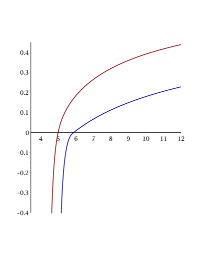
Figure 7. The graphs of the functions $\alpha_{m}(\theta)$ ($\theta>\theta_{m}$) for $k=2$, $q=5$ and $m=1,2$ (see the definition (2.46)). According to formula (2.47) (with $q=5$), $\theta_{1}=1+2\sqrt{3}\doteq 4.4641<\theta_{2}=5$. Note that $\theta_{1}^{0}=5$ and $\theta_{2}^{0}=1+2\mbox{$\>\!$}\sqrt{6}\doteq 5.8990$ are the zeros of $\alpha_{1}(\theta)$ and $\alpha_{2}(\theta)$, respectively (see Example 6.1). Note that the graphs are monotone increasing in line with Conjecture 6.2.

Conjecture 6.2.

For each $m=1,\dots,q-2$, the function $\theta\mapsto\alpha_{m}(\theta)=\ln K_{m}^{*}(\theta)/\ln\theta$ is monotone increasing.

This conjecture is confirmed by computer plots (see Figure 7) and is easy to prove at least for $\theta\leq\theta_{m}^{\mbox{$\>\!$}0}$, where $\theta_{m}^{\mbox{$\>\!$}0}$ is the root of the equation $K_{m}^{*}(\theta)=1$ (cf. Proposition 6.16(a)); that is, $\alpha_{m}(\theta)\leq 0$ for $\theta\leq\theta_{m}^{\mbox{$\>\!$}0}$. Indeed, for any $\theta\in(\theta_{m},\theta_{m}^{\mbox{$\>\!$}0}]$, we have

$$\frac{\mathrm{d}\alpha_{m}(\theta)}{\mathrm{d}\theta} =\frac{\mathrm{d}K_{m}^{*}(\theta)}{\mathrm{d}\theta}\times\frac{1}{\ln\theta\cdot K_{m}^{*}(\theta)}-\frac{\ln K_{m}^{*}(\theta)}{\theta\ln^{2}\theta}>0,$$

because $\mathrm{d}K_{m}^{*}/\mathrm{d}\theta>0$ (Proposition 6.14), whereas $\ln K_{m}^{*}(\theta)\leq\ln K_{m}^{*}(\theta_{m}^{\mbox{$\>\!$}0})=0$.

6.4. Zeros of $\alpha_{\pm}(\theta)$ and $\alpha_{m}(\theta)$

Recall that the functions $\alpha_{\pm}(\theta)$ and $\alpha_{m}(\theta)$ are defined in (2.41) and (2.46), respectively. As was observed in numerical examples (see Figure 3 and also Figures 6 and 7), the functions $\alpha_{-}(\theta)$ and $\alpha_{1}(\theta)$ have the same zero, $\theta_{0}^{-}=\theta_{1}^{0}$, whereas $\alpha_{+}(\theta)=0$ at $\theta^{+}_{0}=1+q/(k-1)$. In this subsection, we give a proof of these observations.

Let us first state and prove a lemma. Recall the notation $L_{m}^{*}(\theta)=\max_{v\in\mathscr{V}_{m}^{+}(\theta)}L_{m}(v;\theta)$ and $K_{m}^{*}(\theta)=\max_{v\in\mathscr{V}_{m}^{+}(\theta)}K_{m}(v;\theta)$.

Lemma 6.15.

Let $q\geq 3$ and $k\geq 2$.

• For any $m\in[1,q-2\mbox{$\>\!$}]$, if $L_{m}(v;\theta)<1$ for some $v\geq 1$ and $\theta>\theta_{m}$ then $K_{m}(v;\theta)<1$.

• Let $1\leq m\leq\frac{1}{2}(q-1)$. If $L_{m}^{*}(\theta)<1$ for some $\theta>\theta_{m}$ then $K_{m}^{*}(\theta)<1$. In particular, $L_{m}^{*}(\theta)=1$ if and only if $K_{m}^{*}(\theta)=1$.

Proof.

(a) Denoting $s:=(L_{m}(v;\theta))^{1/k}\!<1$ and using the definition (5.26), the required inequality $K_{m}(v;\theta)<1$ can be rewritten as

$$p_{k}(v)>\frac{\,s-s^{k}}{\!1-s}=p_{k}(s),$$

and the last inequality holds by monotonicity of $p_{k}(v)$, since $v\geq 1>s$.

(b) Let $v=w_{m}$ be such that $K_{m}(w_{m};\theta)=K_{m}^{*}(\theta)<1$; by Lemma 6.10, $w_{m}\geq 1$. On the other hand, $L_{m}(w_{m};\theta)\leq L_{m}^{*}(\theta)<1$, and by part (a) it follows that $K_{m}(w_{m};\theta)<1$. The last claim in part (b) then follows by continuity and monotonicity of both $L_{m}^{*}(\theta)$ and $K_{m}^{*}(\theta)$ (see Lemma 5.2(b) and Proposition 6.14, respectively), also recalling that $L_{m}(v;\theta)=1$ implies $K_{m}(v;\theta)=1$ (see (5.26)). ∎

Proposition 6.16.

Let $q\geq 3$, and set $m_{0}:=\bigl{\lfloor}\tfrac{1}{2}(q-1)\bigr{\rfloor}$.

• For each $m$ in the range $1\leq m\leq m_{0}$, the function $\alpha_{m}(\theta)$ has a unique zero given by

  $$\theta_{m}^{\mbox{$\>\!$}0}=\frac{m\mbox{$\>\!$}(v_{m}^{\mbox{$\>\!$}0})^{k}+m^{\prime}+1}{p_{k}(v_{m}^{\mbox{$\>\!$}0})},$$ (6.67)

  where $v_{m}^{\mbox{$\>\!$}0}>1$ is a sole positive root of the equation

  $$m\sum_{i=1}^{k-1}i\mbox{$\>\!$}v^{k-i}-(m^{\prime}+1)\sum_{i=1}^{k-1}i\mbox{$\>\!$}v^{i-k}=0.$$ (6.68)

• • The function $\alpha_{+}(\theta)$ has a unique zero given by $\theta^{+}_{0}=1+\frac{q}{k-1}$. Moreover, $\alpha^{\prime}_{+}(\theta^{+}_{0})=0$.

  • The function $\alpha_{-}(\theta)$ has a unique zero $\theta^{-}_{0}$, which coincides with the zero $\theta_{1}^{\mbox{$\>\!$}0}$ of the function $\alpha_{1}(\theta)$.

• The zeros $\theta_{1}^{\mbox{$\>\!$}0},\dots,\theta_{m_{0}}^{\mbox{$\>\!$}0}$ follow in ascending order and are strictly below $\theta_{0}^{+}$,

  $$\theta_{1}^{\mbox{$\>\!$}0}<\dots<\theta_{m_{0}}^{\mbox{$\>\!$}0}<\theta_{0}^{+}=1+\frac{q}{k-1}.$$ (6.69)

Proof.

(a) By the definition (2.46), the condition $\alpha_{m}(\theta)=0$ means that $K_{m}^{*}(\theta)=1$ and hence, by Lemma 6.15(b), $L_{m}^{*}(\theta)=1$. Eliminating $\theta$ from the system of equations $L_{m}(v;\theta)=1$, $\partial L_{m}(v;\mbox{$\>\!$}\theta)/\partial v=0$ gives for the root $v=v_{m}^{\mbox{$\>\!$}0}$ the equation (cf. (5.21))

$$mk\mbox{$\>\!$}v^{k-1}p_{k}(v)-\bigl{(}m\mbox{$\>\!$}v^{k}+m^{\prime}+1\bigr{)}\mbox{$\;\!$}p^{\prime}_{k}(v)=0,$$

which can be rearranged to the form (6.68). Uniqueness of positive solution $v_{m}^{\mbox{$\>\!$}0}$ of the equation (6.68) is obvious, noting that the left-hand side of (6.68) is a continuous, increasing function in $v>0$, with the range from $-\infty$ to $+\infty$. To show that $v_{m}^{\mbox{$\>\!$}0}>1$, it suffices to check that the left-hand side of (6.68) at $v=1$ is negative, which is indeed true since $2m\leq q-1<q$. Expressing $\theta$ from the equation $L_{m}(v^{\mbox{$\>\!$}0}_{m};\theta)=1$, we obtain formula (6.67).

(b) In the limit $\alpha\to 0$, the equation (5.4) always has root $u=1$, while for $u\neq 1$, by virtue of the identity (5.1), it is reduced to equation (5.3) with $m=1$. Using the notation (5.13), the latter equation can be rewritten as $L_{1}(u;\theta)=1$, which in turn has up to two (positive) roots (see Lemma 5.2). In total, there are three positive roots, and for this number to reduce to two (which is the condition of belonging to the curves $y=\alpha_{\pm}(\theta)$), either (i) one zero of the function $u\mapsto L_{1}(u;\theta)-1$ must coincide with $u=1$, or (ii) the equation $L_{1}(u;\theta)=1$ must have a double root, thus also satisfying the condition $\partial L_{1}(u;\theta)/\partial u=0$.

In case (i), the condition $L_{1}(u;\theta)|_{u=1}\mbox{$\;\!\!$}=1$ transcribes as $(\theta-1)(k-1)-(q-1)=1$, which immediately yields the root $\theta_{0}^{+}=1+q/(k-1)$. According to the substitution (5.8) (with $\alpha=0$), the corresponding root of the quadratic equation (2.37) is given by $x=\theta_{0}^{+}/(q-1)$, which appears to be the smaller of the two roots, $x=x_{-}$. Therefore, in view of formulas (2.40) and (2.41), the value $\theta_{0}^{+}$ is a zero of the function $\alpha_{+}(\theta)$. Indeed, using the definition (2.36) of $b=b(\theta)$, the second root of (2.37) is found to be

$$x_{+}=\frac{b}{x_{-}}=\frac{\theta_{0}^{+}\mbox{$\;\!$}(\theta_{0}^{+}+q-2)}{q-1}\cdot\frac{q-1}{\theta_{0}^{+}}=\theta_{0}^{+}+q-2>\frac{\theta_{0}^{+}}{q-1}=x_{-},$$

as claimed.

In case (ii), according to the proof of part (a), the unique solution of the system $L_{1}(u;\theta)=1$, $\partial L_{1}(u;\theta)/\partial u=0$ is given by $(u,\theta)=(v_{1}^{0},\theta_{1}^{\mbox{$\>\!$}0})$, where

$$\theta_{1}^{\mbox{$\>\!$}0}=1+\frac{(v_{1}^{0})^{k}+2}{p_{k}(v_{1}^{0})}$$ (6.70)

and $v_{1}^{0}>1$ is a sole root of the equation (6.68) with $m=1$, that is,

$$\sum_{i=1}^{k-1}i\mbox{$\>\!$}v^{k-i}-(q-1)\sum_{i=1}^{k-1}i\mbox{$\>\!$}v^{i-k}=0.$$ (6.71)

Again by the substitution (5.8) with $\alpha=0$, the corresponding root of the quadratic equation (2.37) is given by

$$x=\frac{\theta_{1}^{\mbox{$\>\!$}0}\mbox{$\;\!$}(v_{1}^{0})^{k}}{q-1},$$

and we wish to prove that this is the bigger of the two roots, $x=x_{+}$, which would imply like before that $\theta_{1}^{\mbox{$\>\!$}0}$ is a zero of the function $\alpha_{-}(\theta)$. Since the other root of (2.37) equals $b/x$, with $b=b(\theta)$ defined in (2.36), our claim is expressed as $x>b/x$, that is,

$$(v_{1}^{0})^{2k}>(q-1)\left(1+\frac{q-2}{\theta_{1}^{\mbox{$\>\!$}0}}\right).$$ (6.72)

Furthermore, recalling that $\theta_{1}^{\mbox{$\>\!$}0}>1$ (see (6.70)), we have

$$1+\frac{q-2}{\theta_{1}^{\mbox{$\>\!$}0}}>q-1,$$

so for the proof of (6.72) it suffices to show that

$$v_{1}^{0}\geq(q-1)^{1/k}.$$ (6.73)

Since the function on the left-hand side of (6.71) is monotone increasing, we only need to check that its value at $v=(q-1)^{1/k}$ is non-positive, that is,

$$\sum_{i=1}^{k-1}i\mbox{$\>\!$}v^{k-i}-\sum_{i=1}^{k-1}i\mbox{$\>\!$}v^{i-k}\leq 0.$$

which can be rewritten as

$$\sum_{i=1}^{k-1}(2\mbox{$\>\!$}i-k)\mbox{$\;\!$}v^{i-k/2}\geq 0.$$

Now, the latter inequality holds because the left-hand side is obviously monotone increasing as a function of $v\geq 1$, being equal to $0$ at $v=1$. Hence, (6.73) follows.

Thus, we have proved that $\theta_{0}^{+}=1+q/(k-1)$ and $\theta_{0}^{-}=\theta_{1}^{\mbox{$\>\!$}0}$ are the sole roots of the functions $\alpha_{+}(\theta)$ and $\alpha_{-}(\theta)$, respectively.

Finally, since the function $\alpha_{+}(\theta)$ is known to be positive both at $\theta_{\rm c}<\theta_{0}^{+}$ and at infinity (see Proposition 6.4), it readily follows that it has a minimum value $0$ at $\theta=\theta_{0}^{+}$, hence $\alpha^{\prime}_{+}(\theta)=0$, as claimed in part (b)(i).

(c) The ordering inequalities between $(\theta_{m}^{0})$ in (6.69) readily follow from the monotonicity property (6.56) proved in Proposition 6.55. Thus, it remains to show that $\theta_{m}^{\mbox{$\>\!$}0}<\theta_{0}^{+}$. Observe that the value $L_{m}(v;\theta)|_{v=1}\mbox{$\;\!\!$}=(\theta-1)\mbox{$\>\!$}(k-1)-(q-1)$ does not depend on $m$. Recalling that $L_{1}(1;\theta_{0}^{+})=1$ (see the proof of part (a)), we get that $L_{m}(1;\theta_{0}^{+})=1$, but

$$\left.\frac{\partial L_{m}(v;\theta_{0}^{+}}{\partial v}\right|_{v=1}\! =(\theta_{0}^{+}-1)\mbox{$\;\!$}p_{k}^{\prime}(1)-mk$$

$$=\frac{q}{k-1}\cdot\frac{k\mbox{$\>\!$}(k-1)}{2}-mk$$

$$=k\left(\frac{q}{2}-m\right)>0,$$

since $m\leq\frac{1}{2}(q-1)<q/2$. Hence, $L_{m}^{*}(\theta_{0}^{+})>L_{m}(1;\theta_{0}^{+})=1$, and by monotonicity of the function $\theta\mapsto L_{m}(v;\theta)$ it follows, according to the proof in part (a), that $\theta_{m}^{\mbox{$\>\!$}0}<\theta_{0}^{+}$.

An alternative simple argument is that, as shown in part (a), the maximum value of $v\mapsto L_{m}(v;\theta_{m}^{\mbox{$\>\!$}0})=1$ is attained at $v=v_{m}^{0}>1$, hence $L_{m}(1;\theta_{m}^{\mbox{$\>\!$}0})<1$ and, again by monotonicity, it follows that $\theta_{0}^{+}>\theta_{m}^{\mbox{$\>\!$}0}$. ∎

A version of Proposition 6.16(b) for $q=2$ is easy to obtain.

Proposition 6.17.

In the case $q=2$, the functions $\alpha_{\pm}(\theta)$ have a unique zero at $\theta_{\rm c}=\frac{k+1}{k-1}$, which coincides with $\theta_{0}^{+}=1+2/(k-1)$. Moreover, $\alpha^{\prime}_{\pm}(\theta_{\rm c}+)=0$.

Proof.

By Lemma 6.3 with $q=2$, we have $\alpha_{-}(\theta)=-\alpha_{+}(\theta)$ for all $\theta\geq\theta_{\rm c}=\frac{k+1}{k-1}$. Thus, it suffices to consider the function $\alpha_{+}(\theta)$. Treating the index $q\geq 2$ as a continuous variable and taking the limit from the domain $q>2$ as $q\to 2+$, we see that the unique zero of $\alpha_{+}(\theta)$, given by $\theta_{0}^{+}(k,q)=1+q/(k-1)$, converges to $1+2/(k-1)=\frac{k+1}{k-1}=\theta_{\rm c}$. On the other hand, the derivative $\alpha^{\prime}_{+}$ vanishes at $\theta_{0}^{+}(k,q)$ for each $q>2$, hence its limiting value at $\theta_{\rm c}$ is also zero, that is, $\alpha^{\prime}_{+}(\theta_{\rm c}+)=0$, as claimed.

This result can also be obtained by a direct calculation. Namely, for $q=2$ the definition (2.36) is reduced to $b(\theta)=\theta^{2}$. From equation (2.37) with $q=2$, it is easy to see that $x_{\pm}(\theta)\to\theta_{\rm c}$ as $\theta\to\theta_{\rm c}+$. Moreover, a simple asymptotic analysis shows that

$$x_{\pm}(\theta)=\theta_{\rm c}\pm\sqrt{2\mbox{$\>\!$}k\mbox{$\>\!$}\theta_{\rm c}\mbox{$\>\!$}(\theta-\theta_{\rm c})}+(k+1)\mbox{$\>\!$}(\theta-\theta_{\rm c})+o(\theta-\theta_{\rm c}),\qquad\theta\to\theta_{\rm c}+.$$

Hence, from (2.40) it follows

$$\ln a_{\pm}(\theta)=-(k+1)\ln\theta_{\rm c}-(k-1)\mbox{$\>\!$}(\theta-\theta_{\rm c})+o(\theta-\theta_{\rm c}),\qquad\theta\to\theta_{\rm c}+.$$

Finally, substituting this into (2.41) we obtain

$$\alpha_{\pm}(\theta) =-(k+1)+\frac{(k+1)\ln\theta_{\rm c}+(k-1)\mbox{$\>\!$}(\theta-\theta_{\rm c})+o(\theta-\theta_{\rm c})}{\ln\theta_{\rm c}+\theta_{\rm c}^{-1}(\theta-\theta_{\rm c})+o(\theta-\theta_{\rm c})}$$

$$=\frac{\theta-\theta_{\rm c}}{\ln\theta_{\rm c}}\left((k-1)-\frac{k+1}{\theta_{\rm c}}\right)+o(\theta-\theta_{\rm c})$$

$$=o(\theta-\theta_{\rm c}),\qquad\theta\to\theta_{\rm c}+,$$

which implies that $\alpha^{\prime}\pm{-}(\theta_{\rm c}+)=0$, as claimed. ∎

Example 6.1.

Consider the case $k=2$. Then the zero of the function $\alpha_{+}(\theta)=0$ specializes to $\theta^{+}_{0}=1+q$. Furthermore, the equation (6.68) is easily solved to yield $v_{m}^{0}=\sqrt{(q-m)/m}$, and from (6.67) we readily find

$$\theta_{m}^{\mbox{$\>\!$}0}=1+2\mbox{$\;\!$}\sqrt{m\mbox{$\>\!$}(q-m)},\qquad 1\leq m\leq\tfrac{1}{2}(q-1).$$ (6.74)

It is of interest to note, by comparing (6.74) with (2.47), that $\theta_{m}^{\mbox{$\>\!$}0}=\theta_{m+1}$ (cf. [30, equation (2.1), page 192]). Finally, taking $m=1$ in (6.74) gives $\theta^{-}_{0}=\theta_{1}^{\mbox{$\>\!$}0}=1+2\mbox{$\;\!$}\sqrt{q-1}$.

Acknowledgements

This research was partially supported by a Royal Society International Exchange Grant IES\R2\181078 (December 2018 – March 2019). U.A.R. acknowledges support by the Institute for Advanced Study of Aix-Marseille University (IMéRA) under a research residency scheme (February–July 2015), by the London Mathematical Society (LMS Scheme 2 visiting grant, Leeds, February 2016), and by the School of Mathematics, University of Leeds (visiting grant, February–March 2016). Research of L.V.B. was partially supported by a visiting grant from SFB 701 (Bielefeld University, June 2015).

Appendix A Proof of Proposition 2.6

Necessity. Assume that the measure $\mu^{h}$ is translation invariant, that is, the condition (2.25) holds. Pick the set $\varLambda\subset V$ to be the unit ball $V_{1}\equiv V_{1}(x_{\circ})=\{x_{\circ},x_{1},\dots,x_{k+1}\}$ centred at the root $x_{\circ}$, with $\partial\{x_{\circ}\}=\{x_{1},\dots,x_{k+1}\}$, where the numbering in $(x_{j})$ is consistent with the bijection $\mathfrak{b}\colon V\to\mathscr{A}_{k}$, that is, $x_{j}=\mathfrak{b}^{-1}(a_{j})$ (see Section 2.3.1). For $z\in V$, the shifted set $V_{1}(z):=\widetilde{T}_{z}(V_{1})=\{z,z_{1},\dots,z_{k+1}\}$ (where $z_{j}=\widetilde{T}_{z}(x_{j})$, $j=1,\dots,k+1$) is the unit ball centred at $z=\widetilde{T}_{z}(x_{\circ})$, so that $\partial\{z\}=\{z_{1},\dots,z_{k+1}\}$. Consider an arbitrary configuration $\varsigma\in\varPhi^{V_{1}}$, with spin values

$$\varsigma(x_{\circ})\mbox{$\>\!\!$}=i_{0},\qquad\varsigma(x_{j})=i_{j},\qquad j=1,\dots,k+1.$$

Note that if $y=\widetilde{T}_{z}(x)$ then, according to (2.24),

$$(\widetilde{T}_{z}\varsigma)(y)=\varsigma\bigl{(}\widetilde{T}^{-1}_{z}(y)\bigr{)}=\varsigma(x).$$ (A.1)

Hence, the property (2.25) of translation invariance of $\mu^{h}$ specializes as follows,

$$\mu^{h}\mbox{$\;\!\!$}\bigl{(}\sigma\in\varPhi^{V}\!\colon\sigma(z)=i_{0},\,\sigma(z_{1})=i_{1},\dots,\,\sigma(z_{k+1})=i_{k+1}\bigr{)}\\ =\mu^{h}\mbox{$\;\!\!$}\bigl{(}\sigma\in\varPhi^{V}\!\colon\sigma(x_{\circ})=i_{0},\,\sigma(x_{1})=i_{1},\dots,\,\sigma(x_{k+1})=i_{k+1}\bigr{)}.$$ (A.2)

Using formulas (1.3) and (1.15), and cancelling the common term $\beta\sum_{j=1}^{k+1}J\mbox{$\>\!$}\delta_{i_{0},i_{j}}$, the equality (A.2) is reduced to

$$\sum_{j=1}^{k+1}\bigl{[}\xi_{i_{j}}(z_{j})+h^{\dagger}_{i_{j}}(z_{j},z)\bigr{]}+\xi_{i_{0}}(z)=\sum_{j=1}^{k+1}\bigl{[}\xi_{i_{j}}(x_{j})+h^{\dagger}_{i_{j}}(x_{j},x_{\circ})\bigr{]}+\xi_{i_{0}}(x_{\circ})+\frac{1}{\beta}\ln\frac{Z_{V_{1}(z)}}{Z_{V_{1}(x_{\circ})}}.$$ (A.3)

Varying $i_{0}\in\varPhi$ in (A.3) (whilst keeping all other $i_{j}$ fixed) shows that the difference $\xi_{i_{0}}(z)-\xi_{i_{0}}(x_{\circ})$ does not depend on $i_{0}$. More precisely, on subtracting from (A.3) the same equality with $i_{0}=q$, we obtain

$$\xi_{i}(z)-\xi_{q}(z)=\xi_{i}(x_{\circ})-\xi_{q}(x_{\circ}),\qquad i=1,\dots,q-1.$$ (A.4)

Since (A.4) holds for any $z\in V$, this proves (2.26) in view of the notation (2.2).

Furthermore, by virtue of (2.26) the equality (A.3) becomes

$$\sum_{j=1}^{k+1}h^{\dagger}_{i_{j}}(z_{j},z)=\sum_{j=1}^{k+1}h^{\dagger}_{i_{j}}(x_{j},x_{\circ})+\!\sum_{x\in V_{1}(x_{\circ})}\!\xi_{q}(x)-\!\sum_{y\in V_{1}(z)}\!\xi_{q}(y)+\frac{1}{\beta}\ln\frac{Z_{V_{1}(z)}}{Z_{V_{1}(x_{\circ})}}.$$ (A.5)

Similarly, varying the values $i_{1},\dots,i_{k+1}$ in (A.5) (one at a time) yields, for each $j=1,\dots,k+1$,

$$\check{h}^{\dagger}_{i}(z_{j},z)=\check{h}^{\dagger}_{i}(x_{j},x_{\circ}),\qquad i=1,\dots,q-1.$$ (A.6)

On the other hand, fix $j\in\{1,\dots,k+1\}$ and consider the shift $\widetilde{T}_{z_{j}}$, resulting in

$$\widetilde{T}_{z_{j}}(x_{\circ})=z_{j},\qquad\widetilde{T}_{z_{j}}(x_{j})=z.$$

The latter equality follows by recalling the definition of conjugate translations (see (2.23)) and noting that $z_{j}=\widetilde{T}_{z}(x_{j})=\mathfrak{b}^{-1}(\mathfrak{b}(z)\mbox{$\>\!$}\mathfrak{b}(x_{j}))=\mathfrak{b}^{-1}(\mathfrak{b}(z)\mbox{$\>\!$}a_{j})$ and, therefore,

$$\widetilde{T}_{z_{j}}(x_{j})=\mathfrak{b}^{-1}(\mathfrak{b}(z_{j})\mbox{$\>\!$}\mathfrak{b}(x_{j}))=\mathfrak{b}^{-1}\mbox{$\;\!\!$}(\mathfrak{b}(z)\mbox{$\>\!$}a_{j}^{2})=\mathfrak{b}^{-1}\mbox{$\;\!\!$}(\mathfrak{b}(z))=z,$$

because $a_{j}^{2}=e$ (see Section 2.3.1). Hence, for $\widetilde{T}_{z_{j}}$ the result (A.6) transforms into

$$\check{h}^{\dagger}_{i}(z,z_{j})=\check{h}^{\dagger}_{i}(x_{j},x_{\circ}),\qquad i=1,\dots,q-1.$$ (A.7)

Comparing (A.6) and (A.7), we conclude that $\check{h}^{\dagger}_{i}(z_{j},z)=\check{h}^{\dagger}_{i}(z,z_{j})$, and the claim (2.27) follows. Finally, let $y=\widetilde{T}_{v}(z)$ and $y_{j}=\widetilde{T}_{v}(z_{j})$, for some $v\in V$. Observe that

$$y=\widetilde{T}_{y}(x_{\circ}),\qquad y_{j}=\widetilde{T}_{y}(x_{j}).$$ (A.8)

The first equality in (A.8) is automatic; to check the second one, note that

$$\mathfrak{b}(y_{j}) =\mathfrak{b}(v)\mbox{$\;\!$}\mathfrak{b}(z_{j}) [y_{j}=\widetilde{T}_{v}(z_{j})]$$

$$=\mathfrak{b}(v)\mbox{$\;\!$}(\mathfrak{b}(z)\mbox{$\>\!$}\mathfrak{b}(x_{j})) [z_{j}=\widetilde{T}_{z}(x_{j})]$$

$$=(\mathfrak{b}(v)\mbox{$\>\!$}\mathfrak{b}(z))\mbox{$\;\!$}\mathfrak{b}(x_{j})$$

$$=\mathfrak{b}(y)\mbox{$\>\!$}\mathfrak{b}(x_{j}) [y=\widetilde{T}_{v}(z)].$$

That is, $\mathfrak{b}(y_{j})=\mathfrak{b}(y)\mbox{$\>\!$}\mathfrak{b}(x_{j})$ and (A.8) follows. Thus, formula (A.6) applied to the edge $\langle y_{j},y\rangle$ gives

$$\check{h}^{\dagger}_{i}(y_{j},y)=\check{h}^{\dagger}_{i}(x_{j},x_{\circ}),\qquad i=1,\dots,q-1.$$

Combined with (A.6), this implies

$$\check{h}^{\dagger}_{i}(z_{j},z)=\check{h}^{\dagger}_{i}(y_{j},y)=\check{h}^{\dagger}_{i}\bigl{(}\widetilde{T}_{v}(z_{j}),\widetilde{T}_{v}(z)\bigr{)},$$

and (2.28) follows. This completes the “only if” part of the proof.

Sufficiency. Suppose that the conditions (2.26), (2.27) and (2.28) are satisfied. It suffices to verify formula (2.25) for the balls $V_{n}$ ($n\geq 1$). For $z\in V$, denote $\varLambda:=\widetilde{T}_{z}(V_{n-1})$, then $\bar{\varLambda}=\widetilde{T}_{z}(V_{n})$ and $\partial\varLambda=\widetilde{T}_{z}(W_{n})$. Furthermore, for $\varsigma\in\varPhi^{V_{n}}$ set $\varsigma_{z}:=\widetilde{T}_{z}(\varsigma)\in\varPhi^{\bar{\varLambda}}$ (see (2.24)). Observe that if $y=\widetilde{T}_{z}(x)$ then, according to (A.1),

$$\varsigma_{z}(y)=\varsigma(\widetilde{T}^{-1}_{z}(y))=\varsigma(x).$$ (A.9)

Hence, recalling (1.3), we have

$$H_{\mbox{$\;\!\!$}\bar{\varLambda}}(\varsigma_{z}) =-\!\!\sum_{\langle y,\mbox{$\>\!$}y^{\prime}\rangle\in E_{\bar{\varLambda}}}\!\!J\mbox{$\>\!$}\delta_{\varsigma_{z}(y),\mbox{$\>\!$}\varsigma_{z}(y^{\prime})}-\sum_{y\in\bar{\varLambda}}\xi_{\varsigma_{z}(y)}(y)$$

$$=-\!\!\sum_{\langle x,\mbox{$\>\!$}x^{\prime}\rangle\in E_{n}}\!\!J\mbox{$\>\!$}\delta_{\varsigma(x),\mbox{$\>\!$}\varsigma(x^{\prime})}-\sum_{x\in V_{n}}\xi_{\varsigma(x)}(\widetilde{T}_{z}(x))$$

$$=H_{n}(\varsigma)+\sum_{x\in V_{n}}\bigl{(}\xi_{q}(x)-\xi_{q}(\widetilde{T}_{z}(x))\bigr{)},$$

where at the last step we used the property (2.26). Thus, from formula (1.15) we obtain, omitting factors not depending on $\varsigma$,

$$\mu^{h}(\sigma_{\mbox{$\;\!\!$}\bar{\varLambda}}\mbox{$\;\!\!$}=\varsigma_{\mbox{$\>\!$}z})\propto\mu^{h}(\sigma_{V_{n}}\mbox{$\;\!\!$}=\varsigma)\cdot\exp\mbox{$\;\!\!$}\Biggl{\{}\beta\mbox{$\;\!\!$}\sum_{y\in\partial\varLambda}\!h^{\dagger}_{\varsigma_{\mbox{$\>\!$}z}(y)}(y,y_{\mbox{$\;\!\!$}\varLambda})-\beta\!\sum_{x\in W_{n}}\!h_{\varsigma(x)}(x)\Biggr{\}},$$ (A.10)

where $y_{\mbox{$\;\!\!$}\varLambda}\mbox{$\;\!\!$}$ is the unique neighbour of $y\in\partial\varLambda$ in $\varLambda$. Note that if $y=\widetilde{T}_{z}(x)$, with $x\in\partial V_{n-1}\mbox{$\>\!\!$}=W_{n}$, then $y_{\mbox{$\;\!\!$}\varLambda}\mbox{$\;\!\!$}=\widetilde{T}_{z}(x^{\prime})$, where $x^{\prime}\in W_{n-1}$ is the unique vertex such that $x\in S(x^{\prime})$. Thus, using (A.9), (2.28) and (2.29), we can write

$$\exp\mbox{$\;\!\!$}\Biggl{\{}\beta\mbox{$\;\!\!$}\sum_{y\in\partial\varLambda}\!h^{\dagger}_{\varsigma_{\mbox{$\>\!$}z}(y)}\mbox{$\;\!\!$}(y,y_{\mbox{$\;\!\!$}\varLambda})\Biggl{\}} =\exp\mbox{$\;\!\!$}\Biggl{\{}\beta\mbox{$\;\!\!$}\sum_{x\in W_{n}}\!h^{\dagger}_{\varsigma(x)}\mbox{$\;\!\!$}\bigl{(}\widetilde{T}_{z}(x),\widetilde{T}_{z}(x^{\prime})\bigr{)}\Biggl{\}}$$

$$\propto\exp\mbox{$\;\!\!$}\Biggl{\{}\beta\mbox{$\;\!\!$}\sum_{x\in W_{n}}\!h^{\dagger}_{\varsigma(x)}(x,x^{\prime})\Biggl{\}}$$

$$\propto\exp\mbox{$\;\!\!$}\Biggl{\{}\beta\mbox{$\;\!\!$}\sum_{x\in W_{n}}\!h_{\varsigma(x)}(x)\Biggl{\}}.$$

Returning to (A.10), this gives $\mu^{h}(\sigma_{\mbox{$\;\!\!$}\bar{\varLambda}}\mbox{$\;\!\!$}=\varsigma_{z})\propto\mu^{h}(\sigma_{V_{n}}\mbox{$\;\!\!$}=\varsigma)$, and since

$$\sum_{\varsigma\in\varPhi^{V_{n}}}\mu^{h}(\sigma_{\mbox{$\;\!\!$}\bar{\varLambda}}\mbox{$\;\!\!$}=\varsigma_{z})=1=\sum_{\varsigma\in\varPhi^{V_{n}}}\mu^{h}(\sigma_{V_{n}}\mbox{$\;\!\!$}=\varsigma),$$

it follows that $\mu^{h}(\sigma_{\mbox{$\;\!\!$}\bar{\varLambda}}\mbox{$\;\!\!$}=\varsigma_{z})=\mu^{h}(\sigma_{V_{n}}\mbox{$\;\!\!$}=\varsigma)$, and the proof of the “if” part is complete.

Appendix B Proof of Lemma 5.3

B.1. Proof of part (a)

Denote $t:=\theta-1$. For $q=3$ (i.e., with $m=m^{\prime}\mbox{$\;\!\!$}=1$), the partial derivative $\partial K_{1}/\partial v$ (see (6.23)) can be represented as

$$\frac{\partial K_{1}}{\partial v} =\frac{(p_{k}+1)^{k-1}}{(p_{k}+L_{m})^{k+1}}\,\biggl{\{}\bigl{(}p_{k}+1+(1-L_{1})(k-1)\bigr{)}L^{\prime}_{1}\mbox{$\>\!$}\bigl{(}p_{k}-(k-1)\bigr{)}$$

$$\qquad-(1-L_{1})\mbox{$\>\!$}k\mbox{$\>\!$}L_{1}\left(p_{k}^{\prime}-\frac{k\mbox{$\>\!$}(k-1)}{2}\right)+\frac{k\mbox{$\>\!$}(k-1)}{2}\mbox{$\>\!$}(1-L_{1})\bigl{(}2L_{1}^{\prime}-kL_{1}\bigr{)}\biggr{\}},$$ (B.1)

where $L_{1}=t\mbox{$\>\!$}p_{k}-v^{k}-1$ and $L_{1}^{\prime}=\partial L_{1}/\partial v=t\mbox{$\>\!$}p^{\prime}_{k}-k\mbox{$\>\!$}v^{k-1}$.

Note that $\partial K_{1}/\partial v|_{v=1}\mbox{$\;\!\!$}=0$ (cf. (6.39)); this follows without calculations from the scaling property $K_{1}(v;t)=K_{1}(v^{-1};t)$ (see (6.15)). More explicitly, using the formulas

$$p_{k}\mbox{$\>\!$}|_{v=1}\mbox{$\;\!\!$}=k-1,\qquad p^{\prime}_{k}\mbox{$\>\!$}|_{v=1}\mbox{$\;\!\!$}=\frac{k\mbox{$\>\!$}(k-1)}{2},$$ (B.2)

it is easy to see that the terms in (B.1) vanish at $v=1$. We will also need the formula

$$p^{\prime\prime}_{k}\mbox{$\>\!$}|_{v=1}\mbox{$\;\!\!$}=\frac{k\mbox{$\>\!$}(k-1)\mbox{$\>\!$}(k-2)}{3}.$$ (B.3)

Such expressions can be obtained by successively differentiating (at $v=1$) the identity

$$v^{k}-1\equiv(v-1)(p_{k}+1).$$

To compute the second-order derivative $\partial^{2}K_{1}/\partial v^{2}$ at $v=1$, we need to differentiate in (B.1) only the factors that vanish at $v=1$, setting $v=1$ elsewhere. Hence,

$$\left.\frac{\partial^{2}K_{1}}{\partial v^{2}}\right|_{v=1} =\frac{(p_{k}+1)^{k-1}}{(p_{k}+L_{1})^{k+1}}\,\biggl{\{}(p_{k}+1)\mbox{$\>\!$}L^{\prime}_{1}\mbox{$\>\!$}p^{\prime}_{k}$$

$$\quad+(1-L_{1})\left[(k-1)\mbox{$\>\!$}L^{\prime}_{1}\mbox{$\>\!$}p^{\prime}_{k}-k\mbox{$\>\!$}L_{1}\mbox{$\>\!$}p_{k}^{\prime\prime}+\frac{k\mbox{$\>\!$}(k-1)}{2}\mbox{$\;\!$}(2L^{\prime\prime}_{1}-kL^{\prime}_{1})\right]\biggr{\}}\biggr{|}_{v=1}.$$ (B.4)

Using (B.2) and (B.3), we find

$$L_{1}|_{v=1} =t\mbox{$\>\!$}p_{k}(1)-2=t\mbox{$\>\!$}(k-1)-2,$$ (B.5)

$$L_{1}^{\prime}|_{v=1} =t\mbox{$\>\!$}p^{\prime}_{k}(1)-k=t\mbox{$\;\!$}\frac{k\mbox{$\>\!$}(k-1)}{2}-k,$$ (B.6)

$$L_{1}^{\prime\prime}|_{v=1} =t\mbox{$\>\!$}p^{\prime\prime}_{k}(1)-k\mbox{$\>\!$}(k-1)=t\mbox{$\;\!$}\frac{k\mbox{$\>\!$}(k-1)\mbox{$\>\!$}(k-2)}{3}-k\mbox{$\>\!$}(k-1).$$ (B.7)

Finally, substituting formulas (B.2), (B.3) and (B.5)–(B.7) into (B.4), after simple manipulations (verified with Maple) we obtain

$$\left.\frac{\partial^{2}K_{1}}{\partial v^{2}}\right|_{v=1} =\left(\frac{k}{(k-1)(t+1)-2}\right)^{k+1}\,\frac{k-1}{2}$$

$$\qquad\times\left(\frac{(k-1)^{2}}{2}\,t^{2}+\frac{(k-1)\mbox{$\>\!$}(7k-11)}{6}\,t-3k+1\right).$$ (B.8)

The quadratic polynomial in (B.8) has one positive zero $t=t^{*}$,

$$t^{*}=\frac{11-7k+\sqrt{49k^{2}+62k+49}}{6\mbox{$\>\!$}(k-1)},$$

which corresponds to $\tilde{\theta}_{1}=t^{*}\!+1$ as defined in (2.48). Hence, $\partial^{2}K_{1}/\partial v^{2}|_{v=1}>0$ for $\theta>\tilde{\theta}_{1}$, which implies that $v=1$ is a local minimum of the function $v\mapsto K_{1}(v;\theta)$. This completes the proof of Lemma 5.3(a).

B.2. Proof of part (b)

It suffices to show, for $1\leq\theta\leq\tilde{\theta}_{1}$ (i.e., $0\leq t\leq t^{*}$), that $v=1$ is the sole root of the equation $\partial K_{1}/\partial v=0$. A plausible general scheme of the proof of the latter statement may be as follows.

• First, the condition $\partial K_{1}/\partial v=0$ (see (6.23)) is reduced to $P(v;t)=0$, where $P(v;t)$ is a polynomial in $v$ (and also a quadratic polynomial in $t$).

• Since $P(1;t)=0$, the quotient $R(v;t)=P(v;t)/(v-1)$ is a polynomial in $v$, and we wish to prove that $R(v;t)<0$ for any $t\leq t^{*}\mbox{$\;\!\!$}$ and all $v\neq 1$.

• According to the proof in Section B.1, the condition $\partial^{2}K_{1}/\partial v^{2}|_{v=1}\leq 0$ is satisfied whenever $R(1;t)\leq 0$; moreover, the critical value $t^{*}\mbox{$\;\!\!$}$ is determined by the quadratic equation $R(1;t^{*})=0$, which implies that $R(1;t)\leq 0$ for $t\in[\mbox{$\>\!$}0,t^{*}]$.

• Bearing in mind the invariance of $K_{1}(v;t)$ under the map $v\mapsto v^{-1}$, it should be possible to represent the polynomial $R(v;t)$ in the form

  $$R(v;t)=\chi(v)\cdot\widetilde{R}(y;t),\qquad y=v+v^{-1}\geq 2,$$

  where $\chi(v)>0$ and $\widetilde{R}(y;t)$ is a polynomial in $y$.

• The crucial step is to show that, for each $t\in[\mbox{$\>\!$}0,t^{*}]$, the function $y\mapsto\widetilde{R}(y;t)$ is monotone decreasing.

• Finally, using steps (3) to (5), for any $y>2$ (i.e., $v\neq 1$) we have

  $$\widetilde{R}(y;t)<\widetilde{R}(2;t)=\frac{R(1;t)}{\chi(1)}\leq 0,\qquad 0\leq t\leq t^{*}.$$

  Hence, for all $t\in[\mbox{$\>\!$}0,t^{*}]$ and $v\neq 1$, we get

  $$R(v;t)=\chi(v)\cdot\widetilde{R}(y;t)<0,$$

  as required.

In what follows, we implement this scheme in more detail for the cases $k=2,3,4$. All calculations were done analytically and also verified using Maple.

B.2.1. Case $k=2$

According to formula (2.49), $t^{*}\mbox{$\;\!\!$}=\frac{1}{2}\bigl{(}\sqrt{41}-1\bigr{)}$. The polynomial $P(v;t)$ is found to be

$$P(v;t) =t^{2}v^{2}-t^{2}v-tv^{3}+4tv^{2}-4tv+t-4v^{3}+2v^{2}-2v+4$$

$$=(v-1)\bigl{\{}t^{2}v-t\mbox{$\;\!$}(v^{2}-3v+1)-(4v^{2}+2v+4)\bigr{\}}.$$

Hence,

$$R(v;t) =t^{2}v-t\mbox{$\;\!$}(v^{2}-3v+1)-(4v^{2}+2v+4$$

$$=v\left(t^{2}-t\left(v-3+\frac{1}{v}\right)-4\left(v+\frac{1}{v}\right)-2\right)$$

$$=v\left(t^{2}-t\mbox{$\>\!$}(y-3)-4y-2\right),$$

where $y=v+v^{-1}$. This gives

$$\widetilde{R}(y;t)=t^{2}-t\mbox{$\>\!$}(y-3)-4y-2=-y\mbox{$\>\!$}(t+4)+t^{2}+3t-2,$$

which is clearly a decreasing function of $y$ for any $t\geq 0$.

B.2.2. Case $k=3$

By (2.49), we have $t^{*}\!=\frac{4}{3}$. The quotient $R(v;t)=P(v;t)/(v-1)$ is explicitly given by

$$R(t,v) =(v+1)(t+3)\bigl{(}2tv^{3}+2tv-2v^{4}-2+5tv^{2}-4v^{3}-4v\bigr{)}$$

$$=v^{2}(v+1)(t+3)\left(2t\left(v+\frac{1}{v}\right)-2\left(v^{2}+\frac{1}{v^{2}}\right)+5t-4\left(v+\frac{1}{v}\right)\right)$$

$$=v^{2}(v+1)(t+3)\bigl{(}2ty-2\mbox{$\>\!$}(y^{2}-2)+5t-4y\bigr{)}.$$

Thus,

$$\widetilde{R}(y;t)=(t+3)\bigl{(}2ty-2\mbox{$\>\!$}(y^{2}-2)+5t-4y\bigr{)},$$

and it is easy to check that this function is decreasing in $y$ for any $t\leq t^{*}\!=\frac{4}{3}$.

B.2.3. Case $k=4$

Elementary but tedious calculations yield

$$R(v;t) =t^{2}\left(3v^{7}+11v^{6}+25v^{5}+30v^{4}+25v^{3}+11v^{2}+3v\right)$$

$$\quad-t\left(3v^{8}+v^{7}-13v^{6}-57v^{5}-72v^{4}-57v^{3}-13v^{2}+v+3\right)$$

$$\qquad-\left(8v^{8}+24v^{7}+48v^{6}+36v^{5}+32v^{4}+36v^{3}+48v^{2}+24v+8\right).$$

Rearranging under the substitution $y=v+v^{-1}$ gives $R(v;t)=v^{4}\mbox{$\>\!$}\widetilde{R}(y;t)$ with

$$\widetilde{R}(y;t) =t^{2}(3y^{3}+11y^{2}+16y+8)$$

$$\quad-t\mbox{$\>\!$}(3y^{4}+y^{3}-25y^{2}-60y-40)$$

$$\qquad-(8y^{4}+24y^{3}+16y^{2}-36y-48).$$ (B.9)

In particular, if $y=2$ then

$$\widetilde{R}(2;t)=12\mbox{$\>\!$}\bigl{(}9\mbox{$\>\!$}t^{2}+17\mbox{$\>\!$}t-22\bigr{)}=0$$

for $t=\frac{1}{18}\bigl{(}\sqrt{1081}-17\bigr{)}=t^{*}$ (cf. (2.49)), as it should be.

Finally, we need to verify that the function $y\mapsto\widetilde{R}(y;t)$ is decreasing for any $t\in[\mbox{$\>\!$}0,t^{*}]$. Unfortunately (but inevitably), technicalities involved in a purely analytic check become quite substantial; however, using Maple to plot the graph of (B.9), with parameter $t$ ranging from $0$ to $t^{*}$, makes the monotonicity evident.

References

• [1] Abou-Chacra, R., Anderson, P.W. and Thouless, D.J. A selfconsistent theory of localization. J. Phys. C 6 (1973), 1734–1752. (doi:10.1088/0022-3719/6/10/009)
• [2] Aizenman, M. and Warzel, S. The canopy graph and level statistics for random operators on trees. Math. Phys. Anal. Geom. 9 (2007), 291–333. (doi:10.1007/s11040-007-9018-3, MR2329431)
• [3] Athreya, S., Bandyopadhyay, A. and Dasgupta, A. Random walks in i.i.d. random environment on Cayley trees. Statist. Probab. Lett. 92 (2014), 39–44. (doi:10.1016/j.spl.2014.04.026, MR3230470)
• [4] Baxter, R.J. Exactly Solved Models in Statistical Mechanics. Academic Press, London, 1982. (MR0690578)
• [5] Beaudin, L., Ellis-Monaghan, J., Pangborn, G. and Shrock, R. A little statistical mechanics for the graph theorist. Discrete Math. 310 (2010), 2037–2053. (doi:10.1016/j.disc.2010.03.011, MR2629922)
• [6] Bethe, H.A. Statistical theory of superlattices. Proc. Roy. Soc. A 150 (1935), 552–575. (doi:10.1098/rspa.1935.0122)
• [7] Bleher, P., Ruiz, J., Schonmann, R.H., Shlosman, S. and Zagrebnov, V. Rigidity of the critical phases on a Cayley tree. Mosc. Math. J. 1 (2001), 345–363. (doi:10.17323/1609-4514-2001-1-3-345-363, MR1877597)
• [8] Bleher, P.M., Ruiz, J. and Zagrebnov, V.A. On the phase diagram of the random field Ising model on the Bethe lattice. J. Stat. Phys. 93 (1998), 33–78. (doi:10.1023/B:JOSS.0000026727.43077.49, MR1656364)
• [9] Bovier, A. Statistical Mechanics of Disordered Systems: A Mathematical Perspective. Cambridge Series in Statistical and Probabilistic Mathematics, 18. Cambridge University Press, Cambridge, 2006. (doi:10.1017/CBO9780511616808, MR2252929)
• [10] Boykov, Y., Veksler, O. and Zabih R. Fast approximate energy minimization via graph cuts. IEEE Trans. Pattern Anal. Machine Intell. 23 (2001), 1222–1239. (doi:10.1109/34.969114)
• [11] Bricmont, J., Kuroda, K. and Lebowitz, J.L. First order phase transitions in lattice and continuous systems: Extension of Pirogov–Sinai theory. Comm. Math. Phys. 101 (1985), 501–538. (doi:10.1007/BF01210743, MR0815198)
• [12] Brookings, T., Carlson, J.M. and Doyle, J. Three mechanisms for power laws on the Cayley tree. Phys. Rev. E 72 (2005), 056120, 18 pp. (doi:10.1103/PhysRevE.72.056120, MR2198305)
• [13] Chen, M.-S., Onsager, L., Bonner, J. and Nagle, J. Hopping of ions in ice. J. Chem. Phys. 60 (1974), 405–419. (doi:10.1063/1.168105660)
• [14] Daskalakis, C., Mossel, E. and Roch, S. Evolutionary trees and the Ising model on the Bethe lattice: a proof of Steel’s conjecture. Probab. Theory Related Fields 149 (2011), 149–189. (doi:10.1007/s00440-009-0246-2, MR2773028)
• [15] Dembo, A., Montanari, A., Sly, A. and Sun, N. The replica symmetric solution for Potts models on $d$-regular graphs. Comm. Math. Phys. 327 (2014), 551–575. (doi:10.1007/s00220-014-1956-6, MR3183409)
• [16] Domb, C. Configurational studies of the Potts models. J. Phys. A 7 (1974), 1335–1348. (doi:10.1088/0305-4470/7/11/013)
• [17] Friedrich, F., Kempe, A., Liebscher, V. and Winkler, G. Complexity penalized $M$-estimation: fast computation. J. Comput. Graph. Statist. 17 (2008), 201–224. (doi:10.1198/106186008X285591, MR2424802)
• [18] Galanis, A., Štefankovič, D., Vigoda, E. and Yang, L. Ferromagnetic Potts model: refined #BIS-hardness and related results. SIAM J. Comput. 45 (2016), 2004–2065. (doi:10.1137/140997580, MR3572375)
• [19] Gandolfo, D., Rahmatullaev, M.M. and Rozikov, U.A. Boundary conditions for translation-invariant Gibbs measures of the Potts model on Cayley trees. J. Stat. Phys. 167 (2017), 1164–1179. (doi:10.1007/s10955-017-1771-5, MR3647056)
• [20] Ganikhodjaev, N.N. Group presentations and automorphisms of the Cayley tree. (Russian) Dokl. Akad. Nauk Respub. Uzbekistan, no. 4 (1994), 3–5.
• [21] Ganikhodjaev, N. and Rozikov, U. On disordered phase in the ferromagnetic Potts model on the Bethe lattice. Osaka J. Math. 37 (2000), 373–383. (http://projecteuclid.org/euclid.ojm/1200789203, MR1772838)
• [22] Georgii, H.-O. Gibbs Measures and Phase Transitions, 2nd ed. De Gruyter Studies in Mathematics, 9. De Gruyter, Berlin, 2011. (MR2807681)
• [23] Green, P.J. and Richardson, S. Hidden Markov models and disease mapping. J. Amer. Statist. Assoc. 97 (2002), 1055–1070. (doi:10.1198/016214502388618870, MR1951259)
• [24] Graner, F. and Glazier, J. Simulation of biological cell sorting using a two-dimensional extended Potts model. Phys. Rev. Lett. 69 (1992), 2013–2017. (doi:10.1103/PhysRevLett.69.2013)
• [25] Grimmett, G. The Random-Cluster Model. Grundlehren der mathematischen Wissenschaften [A Series of Comprehensive Studies in Mathematics], 333. Springer, Berlin, 2006. (doi:10.1007/978-3-540-32891-9, MR2243761)
• [26] Häggström, O. The random-cluster model on a homogeneous tree. Probab. Theory Related Fields 104 (1996), 231–253. (doi:10.1007/BF01247839, MR1373377)
• [27] Kotecký, R. and Shlosman, S.B. First-order phase transitions in large entropy lattice models. Comm. Math. Phys. 83 (1982), 493–515. (doi:10.1007/BF01247839, MR1373377)
• [28] Kramers, H.A. and Wannier, G.H. Statistics of the two-dimensional ferromagnet. Part I. Phys. Rev. 60 (1941), 252–262. (doi:10.1103/PhysRev.60.252, MR0004803)
• [29] Külske, C. and Rozikov, U.A. Fuzzy transformations and extremality of Gibbs measures for the Potts model on a Cayley tree. Random Structures Algorithms 50 (2017), 636–678. (doi:10.1002/rsa.20671, MR3660523)
• [30] Külske, C., Rozikov, U.A. and Khakimov, R.M. Description of the translation-invariant splitting Gibbs measures for the Potts model on a Cayley tree. J. Stat. Phys. 156 (2014), 189–200. (doi:10.1007/s10955-014-0986-y, MR3215122)
• [31] Laanait, L., Messager, A. and Ruiz, J. Phases coexistence and surface tensions for the Potts model. Comm. Math. Phys. 105 (1986), 527–545. (doi:10.1007/BF01238932, MR0852089)
• [32] Magnus, W., Karrass, A. and Solitar, D. Combinatorial Group Theory: Presentations of Groups in Terms of Generators and Relations, 2nd revised ed. Dover, New York, 1976. (MR0422434)
• [33] Martin, P. Potts Models and Related Problems in Statistical Mechanics. Series on Advances in Statistical Mechanics, 5. World Scientific, Singapore, 1991. (doi:10.1142/0983, MR1103994)
• [34] Martinelli, F., Sinclair, A. and Weitz, D. Glauber dynamics on trees: Boundary conditions and mixing time. Comm. Math. Phys. 250 (2004), 301–334. (doi:10.1007/s00220-004-1147-y, MR2094519)
• [35] Martirosian, D.H. Translation invariant Gibbs states in the $q$-state Potts model. Comm. Math. Phys. 105 (1986), 281–290. (doi:10.1007/BF01211103, MR0849209)
• [36] Mézard, M. and Montanari, A. Reconstruction on trees and spin glass transition. J. Stat. Phys. 124 (2006), 1317–1350. (doi:10.1007/s10955-006-9162-3, MR2266446)
• [37] Mézard, M. and Parisi, G. The Bethe lattice spin glass revisited. Eur. Phys. J. B 20 (2001), 217–233. (doi:10.1007/PL00011099, MR1832936)
• [38] Mossel, E. Survey: Information flow on trees. In: Graphs, Morphisms and Statistical Physics (J. Nešetřil and P. Winkler, eds.), DIMACS Series in Discrete Mathematics and Theoretical Computer Science 63, 155–170. Amer. Math. Soc., Providence, RI, 2004. (doi:10.1090/dimacs/063/12, MR2056226)
• [39] Murua, A. and Quintana, F.A. Semiparametric Bayesian regression via Potts model. J. Comput. Graph. Statist. 26 (2017), 265–274. (doi:10.1080/10618600.2016.1172015, MR3640184)
• [40] Ostilli, M. Cayley trees and Bethe lattices: A concise analysis for mathematicians and physicists. Phys. A 391 (2012), 3417–3423. (doi:10.1016/j.physa.2012.01.038, MR2904466)
• [41] Peruggi, F., di Liberto, F. and Monroy, G. The Potts model on Bethe lattices. I. General results. J. Phys. A 16 (1983), 811–827. (doi:10.1088/0305-4470/16/4/018, MR0706197)
• [42] Peruggi, F., di Liberto, F. and Monroy, G. Phase diagrams of the $q$-state Potts model on Bethe lattices. Phys. A 141 (1987), 151–186. (doi:10.1016/0378-4371(87)90267-6, MR0879715)
• [43] Potts, R.B. Some generalized order-disorder transformations. Proc. Cambridge Philos. Soc. 48 (1952), 106–109. (doi:10.1017/S0305004100027419, MR0047571)
• [44] Preston, C.J. Gibbs States on Countable Sets. Cambridge Tracts in Mathematics, 68. Cambridge University Press, London, 1974. (doi:10.1017/CBO9780511897122, MR0474556)
• [45] Reichardt, J. and Bornholdt, S. Detecting fuzzy community structures in complex networks with a Potts model. Phys. Rev. Lett. 93 (2004), Art. 218701, 4 pp. (doi:10.1103/PhysRevLett.93.218701)
• [46] Riva, V. and Cardy, J. Holomorphic parafermions in the Potts model and stochastic Loewner evolution. J. Stat. Mech. Theory Exp. (2006), no. 12, P12001, 19 pp. (doi:10.1088/1742-5468/2006/12/P12001, MR2280251)
• [47] Rozikov, U.A. Gibbs Measures on Cayley Trees. World Scientific, Hackensack, NJ, 2013. (doi:10.1142/8841, MR3185400)
• [48] Rozikov, U.A. Tree-hierarchy of DNA and distribution of Holliday junctions. J. Math. Biol. 75 (2017), 1715–1733. (doi:10.1007/s00285-017-1136-3, MR3712328)
• [49] Rozikov, U.A. and Shoyusupov, Sh.A. Gibbs measures for the SOS model with four states on a Cayley tree. (Russian) Teoret. Mat. Fiz. 149 (2006), no. 1, 18–31; translation in Theor. Math. Phys. 149 (2006), no. 1, 1312–1323. (doi:10.1007/s11232-006-0120-7, MR2297108)
• [50] Rozikov, U.A. and Suhov, Y.M. Gibbs measures for SOS models on a Cayley tree. Infin. Dimens. Anal. Quantum Probab. Relat. Top. 9 (2006), 471–488. (doi:10.1142/S0219025706002494, MR2256506)
• [51] Rudin, W. Principles of Mathematical Analysis, 3rd ed. International Series in Pure and Applied Mathematics. McGraw-Hill, New York, 1976. (MR0385023)
• [52] Sanyal, S. and Glazier, J.A. Viscous instabilities in flowing foams: A Cellular Potts Model approach. J. Stat. Mech. Theory Exp. (2006), no. 10, P10008, 9 pp. (doi:10.1088/1742-5468/2006/10/P10008)
• [53] Schelling, T.C. Dynamic models of segregation. J. Math. Sociology 1 (1971), 143–186. (doi:10.1080/0022250X.1971.9989794)
• [54] Schramm, O. Conformally invariant scaling limits: an overview and a collection of problems. In: Proceedings of the International Congress of Mathematicians (Madrid, August 22–30, 2006), Vol. I, 513–543. Eur. Math. Soc., Zürich, 2007. (doi:10.4171/022-1/20, MR2334202)
• [55] Schulze, C. Potts-like model for ghetto formation in multi-cultural societies. Int. J. Modern Phys. C 16 (2005), 351–355. (doi:10.1142/S0129183105007169)
• [56] Shiryaev, A.N. Probability, 2nd ed. Graduate Texts in Mathematics, 95. Springer, New York, 1996. (doi:10.1007/978-1-4757-2539-1, MR1368405)
• [57] Spitzer, F. Markov random fields on an infinite tree. Ann. Probab. 3 (1975), 387–398. (doi:10.1214/aop/1176996347, MR0378152)
• [58] Sun, L., Chang, Y.F. and Cai, X. A discrete simulation of tumor growth concerning nutrient concentration. Int. J. Modern Phys. B 18 (2004), 2651–2657. (doi:10.1142/S0217979204025853)
• [59] Szabó, A. and Merks, R.M.H. Cellular Potts modeling of tumor growth, tumor invasion, and tumor evolution. Front. Oncol. 3 (2013), Art. 87, 12 pp. (doi:10.3389/fonc.2013.00087)
• [60] Takaishi, T. Simulations of financial markets in a Potts-like model. Int. J. Modern Phys. C 16 (2005), 1311–1317. (doi:10.1142/S0129183105007923)
• [61] Thouless, D.J. Spin-glass on a Bethe lattice. Phys. Rev. Lett. 56 (1986), 1082–1085. (doi:10.1103/PhysRevLett.56.1082)
• [62] Tikare, V. and Cawley, J.D. Application of the Potts model to simulation of Ostwald ripening. J. Amer. Ceramic Soc. 81 (1998), 485–491. (doi:10.1111/j.1151-2916.1998.tb02366.x)
• [63] Weiss, P.R. The application of the Bethe–Peierls method to ferromagnetism. Phys. Rev. 74 (1948), 1493–1504. (doi:10.1103/PhysRev.74.1493)
• [64] Wu, F.Y. The Potts model. Rev. Modern Phys. 54 (1982), 235–268. (doi:10.1103/RevModPhys.54.235, MR0641370)
• [65] Zachary, S. Countable state space Markov random fields and Markov chains on trees. Ann. Probab. 11 (1983), 894–903. (doi:10.1214/aop/1176993439, MR0714953)