Nucleon Structure Functions from the NJL-Model Chiral Soliton

Abstract

We present numerical simulations for unpolarized and polarized structure functions in a chiral soliton model. The soliton is constructed self-consistently from quark fields from which the structure functions are extracted. Central to the project is the implementation of regularizing the Dirac sea (or vacuum) contribution to structure functions from first principles. We discuss in detail how sum rules are realized at the level of the quark wave-functions in momentum space. The comparison with experimental data is convincing for the polarized structure functions but exhibits some discrepancies in the unpolarized case. The vacuum contribution to the polarized structure functions is particularly small.

I Introduction

Perhaps the most convincing evidence for the quark substructure of baryons emerges from Deep Inelastic Scattering (DIS). The conjuction of perturbative Quantum Chromo Dynamics (QCD) and the parton model successfully explains the wealth of DIS data collected over the past decades Muta (1987); Roberts (1990); Ynduráin (1993). However, these are not fully first principle calculations as the hadron wave-functions cannot (yet) be directly computed in QCD. Rather, in the spirit of the parton model, quark distributions are parameterized and subjected to perturbative QCD analysis Pumplin et al. (2002). On the other hand there are many phenomenological models based on various aspects of QCD that (attempt to) describe (static) properties of hadrons with particular focus on the nucleon. Examples are the non-relativistic quark model Kokkedee (1979), the MIT bag model Thomas (1984) relativistic quark-diquark models Maris and Roberts (2003), chiral soliton models Weigel (2008); just to name a few. In principle any of these approaches should also be capable to predict nucleon structure functions. This is particular challenging for chiral soliton models that are formulated as bosonized action functionals hiding the quark substructure of hadrons. In this respect the Nambu-Jona-Lasino (NJL) or chiral quark soliton model Alkofer et al. (1996); Christov et al. (1996) is special: based on a quark self-interaction the bosonization process can be traced step by step.

In the past nucleon structure functions have indeed been computed from the chiral quark soliton model and mainly two approaches were followed. Within the valence quark only approximation Weigel et al. (1997a, b) the observation that though the Dirac sea (or vacuum) is essential to form the soliton, the vacuum contribution to nucleon properties is only moderate thereby justifying neglecting its contribution to the structure functions. Though this approximation has empirical support, it is formally incomplete and does not follow from a systematic expansion scheme. In parallel, studies on the quark distributions were performed Diakonov et al. (1996, 1997); Pobylitsa et al. (1999); Wakamatsu and Kubota (1998, 1999); Wakamatsu (2003a, b) that identified the model quark degrees of freedom with those using the operator product expansion in the analysis of DIS. These studies included vacuum contributions. These are plagued by ultra-violet divergences requiring an a posteriori implementation of regularization by a single Pauli-Villars subtraction imposed onto the distributions. Unfortunately, this is not stringent since there are terms in the action that do not undergo regularization, e.g. to maintain the axial anomaly as measured by the decay of the neutral pion into two photons. Generally, the model has quadratic divergences (most notably the gap equation) and a single subtraction may or may not be sufficient to remove all divergences. In the present project we therefore include the vacuum contributions to the nucleon structure functions (i) without identifying the NJL model quarks field with those of QCD, and (ii) by implementing the mandatory regularization already at the level of the defining action functional. The first issue is addressed by noting that the model emulates the chiral symmetry of QCD and thus produces the same symmetry currents, in particular the electromagnetic one. To address the second issue we recall that DIS is described by the hadronic tensor $W_{\mu\nu}$ which is the Fourier transform of the nucleon matrix element of the commutator of two electromagnetic current operators. Though there is no direct implementation of this commutator when bosonizing the NJL model, we take advantage of its relation to the Compton tensor $T_{\mu\nu}$ which itself is computed from the time-ordered product of these currents. Time-ordered products are straightforwardly included in a path integral formalism within which bosonization is conducted. Regularizing this path integral by multiple Pauli-Villars subtractions proves most appropriate because it allows to trace the quark that carries the large momentum in the Bjorken limit. This formalism was developed already some time ago Weigel et al. (1999) but its numerical simulation has been long outstanding. It will be central to the study presented here.

This paper is organized as follows: In Section II we introduce the NJL model with emphasis on describing the regularization procedure in Minkowski space. The formulation in Minkowski space is advantageous to identify the absorptive part of $T_{\mu\nu}$ which leads to $W_{\mu\nu}$. In Section III we review the formalism from Ref. Weigel et al. (1999) of how to obtain the hadronic tensor in this model and in particular the role of the Bjorken limit. The NJL soliton description is explained in Section IV. We discuss the formalism to obtain the structure functions via the hadronic tensor from quark spinors that self-consistently interact with the soliton in Section V. Subsequently (Section VI) we describe the way in which this formalism builds up the sum rules. Numerical results are presented in Section VII. This analysis also includes the perturbative evolution to the scale at which experimental data are taken. As stressed above, the model structure functions are identified from symmetry currents, not by equating QCD degrees of freedom. However, the evolution makes this unavoidable for the lack of any sensible alternative. We briefly conclude and summarize in Section VIII. Finally we leave technical details to four Appendixes.

Some preliminary results extracted from this paper have been put forward in Ref. Takyi and Weigel (2019)

II The model

We formulate the regularized action of the bosonized Nambu-Jona-Lasino (NJL) model in Minkowski space as the sum of three pieces

$$\mathcal{A}_{\rm NJL} =\mathcal{A}_{\rm R}+\mathcal{A}_{\rm I}+\frac{1}{4G}\int d^{4}x\,{\rm tr}\left[S^{2}+P^{2}+2m_{0}S\right]$$ (1)

$$\mathcal{A}_{\rm R} =-i\frac{N_{C}}{2}\sum_{i=0}^{2}c_{i}{\rm Tr}\,{\rm log}\left[-\mathbf{D}\mathbf{D}_{5}+\Lambda_{i}^{2}-i\epsilon\right]\,,$$ (2)

$$\mathcal{A}_{\rm I} =-i\frac{N_{C}}{2}{\rm Tr}\,{\rm log}\left[-\mathbf{D}\left(\mathbf{D}_{5}\right)^{-1}-i\epsilon\right]\,.$$

The subscripts $R$ and $I$ for real and imaginary refer to the respective properties after Wick-rotation to Euclidean space. In Minkowski space this corresponds to the use of two distinct Dirac operators

$$\mathbf{D} ={\rm i}\partial\hskip-5.0pt/-\left(S+{\rm i}\gamma_{5}P\right)+v\hskip-5.0pt/+a\hskip-5.0pt/\gamma_{5}=:\mathbf{D}^{(\pi)}+v\hskip-5.0pt/+a\hskip-5.0pt/\gamma_{5}$$ (3)

$$\mathbf{D}_{5} =-{\rm i}\partial\hskip-5.0pt/-\left(S+{\rm i}\gamma_{5}P\right)-v\hskip-5.0pt/+a\hskip-5.0pt/\gamma_{5}=:\mathbf{D}_{5}^{(\pi)}+v\hskip-5.0pt/+a\hskip-5.0pt/\gamma_{5}\,.$$ (4)

Here, as in the local part of Eq. (1), $S$ and $P$ are scalar and pseudoscalar fields that represent physical particles. Furthermore $v_{\mu}$ and $a_{\mu}$ are source fields. When expanding the action with respect to these sources the linear terms couple to the vector and axial vector currents. Since $\mathcal{A}_{\rm I}$ is (conditionally) finite in the ultra-violet, only $\mathcal{A}_{\rm R}$ undergoes regularization. Its dynamical content is quadratically divergent and we thus require two subtractions. In the Pauli-Villars scheme they are implemented as

$$c_{0}=1\,,\quad\Lambda_{0}=0\,,\quad\sum_{i=0}^{2}c_{i}=0\quad{\rm and}\quad\sum_{i=0}^{2}c_{i}\Lambda_{i}^{2}=0\,.$$ (5)

In practice we will reduce the number of regularization parameters by assuming $\Lambda_{1}\to\Lambda_{2}=\Lambda$ which translates into the general prescription $\sum_{i}c_{i}f(\Lambda_{i}^{2})=f(0)-f(\Lambda^{2})+\Lambda^{2}f^{\prime}(\Lambda^{2})$. Nevertheless we always write the regularization as in Eq. (1).

The variation of the action with respect to the scalar field $S$ yields the gap equation

$$\frac{1}{2G}\left(m-m_{0}\right)=-4iN_{C}m\sum_{i=0}^{2}c_{i}\int\frac{d^{4}k}{(2\pi)^{4}}\left[-k^{2}+m^{2}+\Lambda_{i}^{2}-i\epsilon\right]^{-1}$$ (6)

that determines the vacuum expectation value of the scalar field $\langle S\rangle=m$. Replacing $S$ by $\langle S\rangle$ in $\mathbf{D}$ shows that $m$ is the fermion mass and is thus called the constituent quark mass. The chiral field $U$ defines the non-linear representation for the isovector pion field ${\boldsymbol{\pi}}$

$$S+{\rm i}P=mU=m\,{\rm exp}\left[{\rm i}\frac{g}{m}{\boldsymbol{\pi}}\cdot{\boldsymbol{\tau}}\right]\,.$$ (7)

We obtain the pion propagator by expanding $\mathcal{A}$ to quadratic order and extract the pion mass from the pole

$$m_{\pi}^{2}=\frac{1}{2G}\frac{m_{0}}{m}\frac{1}{2N_{C}\Pi(m_{\pi}^{2})}$$ (8)

and requiring a unit residuum at the pole fixes the quark-pion coupling

$$\frac{1}{g^{2}}=4N_{C}\frac{d}{dq^{2}}\left[q^{2}\Pi(q^{2})\right]\Bigg{|}_{q^{2}=m_{\pi}^{2}}\,.$$ (9)

The above polarization function is

$$\Pi(q^{2})=\int_{0}^{1}dx\,\Pi(q^{2},x)\qquad{\rm with}\qquad\Pi(q^{2},x)=-i\sum_{i=0}^{2}c_{i}\,\frac{d^{4}k}{(2\pi)^{4}}\,\left[-k^{2}-x(1-x)q^{2}+m^{2}+\Lambda_{i}^{2}-i\epsilon\right]^{-2}\,.$$ (10)

Finally we get the pion decay constant $f_{\pi}$ from the coupling to the axial current. To this end we expand $\mathcal{A}$ to linear order in both ${\boldsymbol{\pi}}$ and $a_{\mu}$. The result is $f_{\pi}=4N_{C}mg\Pi(m_{\pi}^{2})$. Using the empirical data $m_{\pi}=138{\rm MeV}$ and $f_{\pi}=93{\rm MeV}$ fixes two of the three ($m_{0}$, $G$ and $\Lambda$) model constants. It is customary to use the constituent quark mass $m$ as the single tunable parameter.

III Structure functions in the NJL model

The hadronic tensor of DIS is the matrix element of the commutator of electro-magnetic current operators

$$W_{\mu\nu}(q;H)=\frac{1}{4\pi}\int d^{4}x\,{\rm e}^{{\rm i}q\cdot\xi}\,\Big{\langle}H\Big{|}[J_{\mu}(\xi),J_{\nu}^{\dagger}(0)]\Big{|}H\Big{\rangle}\,,$$ (11)

where $q$ is the momentum of the virtual photon and $H$ refers to either the pion or the nucleon target. This tensor is decomposed into Lorentz structures whose coefficients are form factors that turn into the structure functions in the so-called Bjorken limit. Labeling the target momentum by $p$ this limit is defined as

$$Q^{2}=-q^{2}\to\infty\qquad{\rm with}\quad x=\frac{Q^{2}}{2p\cdot q}\quad{\rm fixed}\,.$$ (12)

Often $x$ is referred to as the Bjorken variable.

By the optical theorem, $W_{\mu\nu}$ is proportional to the absorptive part of the Compton amplitude

$$W_{\mu\nu}(q;H)=\frac{1}{2\pi}\,{\rm Im}\,T_{\mu\nu}(q;H)\,.$$ (13)

The latter is the matrix element of a time-ordered product of the currents

$$T_{\mu\nu}(q;H)={\rm i}\int d^{4}\xi{\rm e}^{{\rm i}q\cdot\xi}\,\Big{\langle}H\Big{|}T\left\{J_{\mu}(\xi)J_{\nu}^{\dagger}(0)\right\}\Big{|}H\Big{\rangle}\,.$$ (14)

With this relation we implement regularization from first principles because the time-ordered product is immediately obtained from the action by functional differentiation

$$T\left\{J_{\mu}(\xi)J_{\nu}(0)\right\}=\frac{\delta^{2}}{\delta v^{\mu}(\xi)\delta v^{\nu}(0)}\mathcal{A}_{\rm NJL}(v)\Bigg{|}_{v_{\mu}=0}\,,$$ (15)

where $v_{\mu}$ is the photon field introduced by minimal coupling. Within the NJL model the photon couples to the quarks inside the hadron. As discussed comprehensively in Ref. Weigel et al. (1999) the evaluation of $T_{\mu\nu}$ becomes feasible in the Bjorken limit. Then the quark propagator that carries the large photon momentum can be identified and thus be taken to be that of a free massless fermion. Thus the functional derivative from Eq. (15) when applied to the real part simplifies to differentiating

$$\mathcal{A}_{\Lambda,{\rm R}}^{(2,v)}=-i\frac{N_{C}}{4}\sum_{i=0}^{2}c_{i}{\rm Tr}\,\left\{\left(-\mathbf{D}^{(\pi)}\mathbf{D}^{(\pi)}_{5}+\Lambda_{i}^{2}\right)^{-1}\left[{\cal Q}^{2}v\hskip-5.0pt/\left(\partial\hskip-5.0pt/\right)^{-1}v\hskip-5.0pt/\mathbf{D}^{(\pi)}_{5}-\mathbf{D}^{(\pi)}(v\hskip-5.0pt/\left(\partial\hskip-5.0pt/\right)^{-1}v\hskip-5.0pt/)_{5}{\cal Q}^{2}\right]\right\}.$$ (16)

At this point it is important to explain the crucial role of the subscript ‘5’ attached to the second term in square brackets of Eq. (16). For this second term we have to recall that the (inverse) derivative operator in $v\hskip-5.0pt/\left(\partial\hskip-5.0pt/\right)^{-1}v\hskip-5.0pt/$ is actually associated with the expansion of $\mathbf{D}_{5}$. When comparing this $\gamma_{5}$–odd operator to the ordinary Dirac operator in Eq. (4) one observes immediately that $\mathbf{D}_{5}$ has a relative sign between the derivative operator $i\partial\hskip-5.0pt/$ and the axial source $a\hskip-5.0pt/\gamma_{5}$. Therefore the axial–vector component of $(v\hskip-5.0pt/\left(\partial\hskip-5.0pt/\right)^{-1}v\hskip-5.0pt/)_{5}$ requires a relative sign. With $S_{\mu\rho\nu\sigma}=g_{\mu\rho}g_{\nu\sigma}+g_{\rho\nu}g_{\mu\sigma}-g_{\mu\nu}g_{\rho\sigma}$, that is

$$\gamma_{\mu}\gamma_{\rho}\gamma_{\nu}=S_{\mu\rho\nu\sigma}\gamma^{\sigma}-i\epsilon_{\mu\rho\nu\sigma}\gamma^{\sigma}\gamma^{5}\quad{\rm while}\quad(\gamma_{\mu}\gamma_{\rho}\gamma_{\nu})_{5}=S_{\mu\rho\nu\sigma}\gamma^{\sigma}+i\epsilon_{\mu\rho\nu\sigma}\gamma^{\sigma}\gamma^{5}\,.$$ (17)

In Ref. Weigel et al. (1999) this modification was formally shown to be consistent with the affected sum rules. In Section VI we see on the level of the momentum space quark wave-functions that the structure functions computed on the basis of Eq. (17) indeed fulfill the sum rules.

Similarly, in the Bjorken limit, the imaginary part becomes

$$\mathcal{A}_{\Lambda,{\rm I}}^{(2,v)}=-i\frac{N_{C}}{4}{\rm Tr}\,\left\{\left(-\mathbf{D}^{(\pi)}\mathbf{D}^{(\pi)}\right)^{-1}\left[{\cal Q}^{2}v\hskip-5.0pt/\left(\partial\hskip-5.0pt/\right)^{-1}v\hskip-5.0pt/\mathbf{D}^{(\pi)}_{5}+\mathbf{D}^{(\pi)}(v\hskip-5.0pt/\left(\partial\hskip-5.0pt/\right)^{-1}v\hskip-5.0pt/)_{5}{\cal Q}^{2}\right]\right\}\,.$$ (18)

These expression are still quite formal and we will use them to obtain nucleon structure functions in Section V. We emphasize that these expressions are directly deducted from the regularized action in Eq. (1) and that no further assumption about the regularization has been made.

In Ref. Weigel et al. (1999) it has been shown that applying this formalism to the pion relates its structure function to the spectral function from Eq. (10) as $F(x)=\frac{5}{9}(4N_{C}g^{2})\frac{d}{dp^{2}}\left[p^{2}\Pi(p^{2},x)\right]\Big{|}_{p^{2}=m_{\pi}^{2}}$, a result that was previously obtained from the analysis of the handbag diagram in Refs. Frederico and Miller (1994); Davidson and Ruiz Arriola (1995).

IV NJL model soliton

We construct the soliton from static meson configurations by introducing a Dirac Hamiltonian $h$ via

$${\rm i}\mathbf{D}^{(\pi)}=\beta({\rm i}\partial_{t}-h)\quad{\rm and}\quad{\rm i}\mathbf{D}^{(\pi)}_{5}=(-{\rm i}\partial_{t}-h)\beta\,.$$ (19)

Its diagonalization

$$h\Psi_{\alpha}=\epsilon_{\alpha}\Psi_{\alpha}\,,$$ (20)

yields eigen-spinors $\Psi_{\alpha}=\sum_{\beta}V_{\alpha\beta}\Psi^{(0)}_{\alpha}$ ($\Psi^{(0)}_{\alpha}$ are free Dirac spinors in a spherical basis, see Appendix A) and energy eigenvalues $\epsilon_{\alpha}$. The hedgehog configuration minimizes the action in the unit baryon number sector and introduces the chiral angle $\Theta(r)$ via

$$h={\boldsymbol{\alpha}}\cdot{\boldsymbol{p}}+\beta\,m\,U_{5}({\boldsymbol{r}})\qquad{\rm where}\qquad U_{5}({\boldsymbol{r}})={\rm exp}\left[{\rm i}\hat{{\boldsymbol{r}}}\cdot{\boldsymbol{\tau}}\,\gamma_{5}\Theta(r)\right]\,.$$ (21)

With the boundary conditions $\Theta(0)=-\pi$ and $\lim_{r\to\infty}\Theta(r)=0$ the diagonalization, Eq. (20) yields a distinct, strongly bound level, $\Psi_{\rm v}$, referred to as the valence quark level Alkofer et al. (1996). Its (explicit) occupation ensures unit baryon number. The functional trace in $\mathcal{A}_{R}$ is computed as an integral over the time interval $T$ and a discrete sum over the basis levels defined by Eq. (20). In the limit $T\to\infty$ the vacuum contribution to the static energy is then extracted from $\mathcal{A}_{R}\to-TE_{\rm vac}$. Collecting pieces, we obtain the total energy functional as Alkofer et al. (1996); Christov et al. (1996)

$$E_{\rm tot}[\Theta]=\frac{N_{C}}{2}\left[1+{\rm sign}(\epsilon_{\rm v})\right]\epsilon_{\rm v}-\frac{N_{C}}{2}\sum_{i=0}^{2}c_{i}\sum_{\alpha}\left\{\sqrt{\epsilon_{\alpha}^{2}+\Lambda_{i}^{2}}-\sqrt{\epsilon_{\alpha}^{(0)2}+\Lambda_{i}^{2}}\right\}+m_{\pi}^{2}f_{\pi}^{2}\int d^{3}r\,\left[1-{\rm cos}(\Theta)\right]\,.$$ (22)

Here we have also subtracted the vacuum energy associated with the non-dynamical meson field configuration $\Theta\equiv 0$ (denoted by the superscript) that is often called the cosmological constant contribution. This subtraction will also play an important role for the unpolarized isosinglet structure function as it enters via the momentum sum rule. The soliton profile is then obtained as the profile function $\Theta(r)$ that minimizes the total energy $E_{\rm tot}$ self-consistently subject to the above mentioned boundary conditions.

This soliton represents an object which has unit baryon number but neither good quantum numbers for spin and flavor (isospin). Such quantum numbers are generated by canonically quantizing the time-dependent collective coordinates $A(t)$ which parameterize the spin-flavor orientation of the soliton. For a rigidly rotating soliton the Dirac operator becomes, after transforming to the flavor rotating frame Reinhardt (1989),

$${\rm i}\mathbf{D}^{(\pi)}=A\beta\left({\rm i}\partial_{t}-{\boldsymbol{\Omega}}\cdot{\boldsymbol{\tau}}-h\right)A^{\dagger}\quad{\rm and}\quad{\rm i}\mathbf{D}^{(\pi)}_{5}=A\left(-{\rm i}\partial_{t}+{\boldsymbol{\Omega}}\cdot{\boldsymbol{\tau}}-h\right)\beta A^{\dagger}\,.$$ (23)

Actual computations involve an expansion with respect to the angular velocities

$$A^{\dagger}\frac{d}{dt}A=\frac{{\rm i}}{2}{\boldsymbol{\Omega}}\cdot{\boldsymbol{\tau}}\,,$$ (24)

which, according to the quantization rules, are replaced by the spin operator

$${\boldsymbol{\Omega}}\longrightarrow\frac{1}{\alpha^{2}}\,{\boldsymbol{J}}\,.$$ (25)

The constant of proportionality is the moment of inertia

$$\alpha^{2}=\frac{N_{C}}{4}\left[1+{\rm sign}(\epsilon_{\rm v})\right]\sum_{\beta\neq{\rm v}}\frac{|\langle{\rm v}|\tau_{3}|\beta\rangle|^{2}}{\epsilon_{\beta}-\epsilon_{\rm v}}+\frac{N_{C}}{8}\sum_{\alpha\neq\beta}\sum_{i=1}^{2}c_{i}\frac{|\langle\alpha|\tau_{3}|\beta\rangle|^{2}}{\epsilon_{\alpha}^{2}-\epsilon_{\beta}^{2}}\left\{\frac{\epsilon_{\alpha}^{2}+\epsilon_{\alpha}\epsilon_{\beta}+2\Lambda_{i}^{2}}{\sqrt{\epsilon_{\alpha}^{2}+\Lambda_{i}^{2}}}-\frac{\epsilon_{\beta}^{2}+\epsilon_{\alpha}\epsilon_{\beta}+2\Lambda_{i}^{2}}{\sqrt{\epsilon_{\beta}^{2}+\Lambda_{i}^{2}}}\right\}\,,$$ (26)

which is of the order $N_{C}$. With Eq. (25) the expansion in ${\boldsymbol{\Omega}}$ is thus equivalent to the one in $1/N_{C}$. The nucleon wave-function becomes a (Wigner D) function of the collective coordinates. A useful relation in computing matrix elements of nucleon states is Adkins et al. (1983)

$$\langle N|\frac{1}{2}{\rm tr}\left(A^{\dagger}\tau_{i}A\tau_{j}\right)|N\rangle=-\frac{4}{3}\langle N|I_{i}J_{j}|N\rangle\,.$$ (27)

V Structure functions from soliton

We first repeat the relation between the structure functions and the hadronic tensor of the nucleon. Its symmetric combination $W_{\mu\nu}^{S}(q)=\frac{1}{2}\left(W_{\mu\nu}(q)+W_{\nu\mu}(q)\right)$, is parameterized by two form factors

$$W_{\mu\nu}^{S}(q) =MW_{1}(\nu,Q^{2})\left(-g_{\mu\nu}+\frac{q_{\mu}q_{\nu}}{q^{2}}\right)+\frac{W_{2}(\nu,Q^{2})}{M}\left(p_{\mu}-\frac{p\cdot q}{q^{2}}q_{\mu}\right)\left(p_{\nu}-\frac{p\cdot q}{q^{2}}q_{\nu}\right)\,.$$ (28)

In the Bjorken limit, Eq. (12), these form factors turn into the unpolarized structure functions that we extract by appropriate projections:

$$F_{1}(x)=-\frac{1}{2}g^{\mu\nu}W_{\mu\nu}^{S}(q)\qquad{\rm and}\qquad\quad F_{2}(x)=-xg^{\mu\nu}W_{\mu\nu}^{S}(q).$$ (29)

It must be noted that the Callan Gross relation, i.e. $F_{1}(x)=2xF_{2}(x)$, is satisfied in this case by construction. Similarly, the anti-symmetric part is also parameterized by two form factors

$$W_{\mu\nu}^{A}(q) ={\rm i}\epsilon_{\mu\nu\lambda\sigma}q^{\lambda}\left\{MG_{1}(\nu,Q^{2})s^{\sigma}+\frac{G_{2}(\nu,Q^{2})}{M}\left((p\cdot q)s^{\sigma}-(q\cdot s)p^{\sigma}\right)\right\}.$$ (30)

In the Bjorken limit these form factors yield the structure functions

$$\mathsf{g}_{1}(x)=M^{2}\nu G_{1}(\nu,Q^{2})\qquad{\rm and}\qquad\mathsf{g}_{2}(x)=M\nu G_{2}(\nu,Q^{2})\,.$$ (31)

The longitudinal, $\mathsf{g}_{1}(x)$, and transverse, $\mathsf{g}_{T}(x)=\mathsf{g}_{1}(x)+\mathsf{g}_{2}(x)$, structure functions are extracted from the hadronic tensor using the projection operators

$$\mathsf{g}_{1}(x)=\frac{{\rm i}}{2M}\epsilon^{\mu\nu\rho\sigma}\frac{q_{\sigma}p_{\rho}}{q\cdot s}W_{\mu\nu}^{A}(q)\quad\text{and}\quad{\boldsymbol{q}}\parallel{\boldsymbol{s}}$$ (32)

$$\mathsf{g}_{T}(x)=\frac{-{\rm i}}{2M}\epsilon^{\mu\nu\rho\sigma}s_{\rho}p_{\sigma}W_{\mu\nu}^{A}(q)\quad\text{and}\quad{\boldsymbol{q}}\perp{\boldsymbol{s}}.$$ (33)

To obtain the hadronic tensor for the nucleon in the soliton model, the functional traces in Eqs. (16) and (18) are computed using the basis defined by the self-consistent soliton, Eq. (20). This calculation has been detailed in Ref. Weigel et al. (1999) that we adopt directly. We start with the leading order in $\frac{1}{N_{C}}$ to the vacuum (or sea) contribution to $W_{\mu\nu}$

$$W^{\rm(s)}_{\mu\nu}(q) =-{\rm i}\frac{MN_{c}\pi}{8}\int\frac{d\omega}{2\pi}\sum_{\alpha}\int d^{3}\xi\int\frac{d\lambda}{2\pi}\,{\rm e}^{{\rm i}Mx\lambda}$$ (34)

$$\hskip 22.76228pt\times\Big{\langle}N,{\boldsymbol{s}}\Big{|}\Bigl{\{}\Bigl{[}\overline{\Psi}_{\alpha}({\boldsymbol{\xi}})\mathcal{Q}_{A}^{2}\gamma_{\mu}n\hskip-5.0pt/\gamma_{\nu}\Psi_{\alpha}({\boldsymbol{\xi}}+\lambda\hat{e}_{3}){\rm e}^{-{\rm i}\lambda\omega}-\overline{\Psi}_{\alpha}({\boldsymbol{\xi}})\mathcal{Q}_{A}^{2}\gamma_{\nu}n\hskip-5.0pt/\gamma_{\mu}\Psi_{\alpha}({\boldsymbol{\xi}}-\lambda\hat{e}_{3}){\rm e}^{{\rm i}\lambda\omega}\Bigr{]}\left.f_{\alpha}^{+}(\omega)\right|_{\rm p}$$ (35)

$$\hskip 34.14322pt+\Bigl{[}\overline{\Psi}_{\alpha}({\boldsymbol{\xi}})\mathcal{Q}_{A}^{2}\left(\gamma_{\mu}n\hskip-5.0pt/\gamma_{\nu}\right)_{5}\Psi_{\alpha}({\boldsymbol{\xi}}-\lambda\hat{e}_{3}){\rm e}^{-{\rm i}\lambda\omega}-\overline{\Psi}_{\alpha}({\boldsymbol{\xi}})\mathcal{Q}_{A}^{2}\left(\gamma_{\nu}n\hskip-5.0pt/\gamma_{\mu}\right)_{5}\Psi_{\alpha}({\boldsymbol{\xi}}+\lambda\hat{e}_{3}){\rm e}^{{\rm i}\lambda\omega}\Bigr{]}\left.f_{\alpha}^{-}(\omega)\right|_{\rm p}\Bigr{\}}\Big{|}N,{\boldsymbol{s}}\hskip 2.84544pt\Big{\rangle}\,.$$

Here $n^{\mu}=\left(1,0,0,1\right)^{\mu}$ is the light-cone vector of the photon momentum while $\mathcal{Q}_{A}=A^{\dagger}\mathcal{Q}A$ denotes the flavor rotated quark charge matrix from which we compute nucleon matrix elements as in Eq. (27). Furthermore

$$f_{\alpha}^{\pm}=\sum_{i=0}^{2}c_{i}\frac{\omega\pm\epsilon_{\alpha}}{\omega^{2}-\epsilon_{\alpha}^{2}-\Lambda_{i}^{2}+{\rm i}\epsilon}\pm\frac{\omega\pm\epsilon_{\alpha}}{\omega^{2}-\epsilon_{\alpha}^{2}+{\rm i}\epsilon},$$ (36)

are Pauli-Villars regularized spectral functions. The subscript ‘$p$’ indicates their pole contributions that we will explain below.

For the vacuum contribution to the isosinglet unpolarized structure function we then obtain

$$\left[F_{1}^{I=0}(x)\right]_{s} ={\rm i}\frac{5\pi}{72}MN_{c}\int\frac{d\omega}{2\pi}\sum_{\alpha}\int\frac{d\lambda}{2\pi}{\rm e}^{{\rm i}Mx\lambda}\left(\sum_{i=0}^{2}c_{i}\frac{\omega+\epsilon_{\alpha}}{\omega^{2}-\epsilon_{\alpha}^{2}-\Lambda_{i}^{2}+{\rm i}\epsilon}\right)_{\rm p}$$ (37)

$$\times\int d^{3}\xi\,\Bigl{\{}\Psi_{\alpha}^{\dagger}({\boldsymbol{\xi}})(1-\alpha_{3})\Psi_{\alpha}({\boldsymbol{\xi}}+\lambda\hat{e}_{3}){\rm e}^{-{\rm i}\omega\lambda}-\Psi_{\alpha}^{\dagger}({\boldsymbol{\xi}})(1-\alpha_{3})\Psi_{\alpha}({\boldsymbol{\xi}}-\lambda\hat{e}_{3}){\rm e}^{{\rm i}\omega\lambda}\Bigr{\}}.$$ (38)

Here the pole contributions is

$$\left(\sum_{i=0}^{2}c_{i}\frac{1}{\omega^{2}-\epsilon_{\alpha}^{2}-\Lambda_{i}^{2}+{\rm i}\epsilon}\right)_{\rm p} =\sum_{i=0}^{2}c_{i}\frac{-{\rm i}\pi}{\omega_{\alpha}}\left[\delta\left(\omega+\omega_{\alpha}\right)+\delta\left(\omega-\omega_{\alpha}\right)\right]\,,$$ (39)

where (eventually we take the single cut-off limit as described after Eq. (5) and thus omit the label $i$ on $\omega_{\alpha}$)

$$\omega_{\alpha}=\sqrt{\epsilon_{\alpha}^{2}+\Lambda_{i}^{2}}\,.$$ (40)

We recall that the single cut-off approach requires a derivative with respect to that cut-off. Of course, this also affects the implicit dependence of $\omega_{\alpha}$ on that cut-off.

We introduce the Fourier transform of the quark wave-function as

$$\widetilde{\Psi}_{\alpha}({\boldsymbol{p}})=\int\frac{d^{3}r}{4\pi}\,\Psi_{\alpha}({\boldsymbol{r}}){\rm e}^{{\rm i}{\boldsymbol{r}}\cdot{\boldsymbol{p}}}.$$ (41)

Implementing a full Fourier transform differs from the approaches of Refs. Wakamatsu and Kubota (1998); Pobylitsa et al. (1999) who used the expansion from diagonalizing the Dirac Hamiltonian, Eq. (20). This resulted in discontinuities of the numerically computed quark distributions and required a smoothening procedure.

Performing the frequency ($\omega$) and lambda ‘$\lambda$’ integrals gives the vacuum contribution of the flavor-singlet unpolarized structure function in the nucleon rest frame (RF)

$$\left[F_{1}^{I=0}(x)\right]_{\rm s}^{\mp} =\frac{5MN_{c}}{144}\sum_{\alpha}\sum_{i=0}^{2}c_{i}\int_{|Mx_{\alpha}^{\pm}|}^{\infty}p\,dp\,\int d\Omega_{p}\Biggl{\{}\pm\widetilde{\Psi}_{\alpha}^{\dagger}({\boldsymbol{p}})\widetilde{\Psi}_{\alpha}({\boldsymbol{p}})-\frac{\epsilon_{\alpha}}{\omega_{\alpha}}\frac{Mx_{\alpha}^{\pm}}{p}\widetilde{\Psi}_{\alpha}^{\dagger}({\boldsymbol{p}})\hat{{\boldsymbol{p}}}\cdot{\boldsymbol{\alpha}}\widetilde{\Psi}_{\alpha}({\boldsymbol{p}})\Biggr{\}},$$ (42)

where

$$Mx_{\alpha}^{\pm}=Mx\pm\omega_{\alpha}.$$ (43)

In the above $[F_{1}^{I=0}(x)]_{\rm s}^{\pm}$ refers to the positive (negative) frequency components that are typically referred to as quark and antiquark distributions. In our calculation they arise from the two poles of the $\delta$-function in Eq. (39). Then the vacuum part of the isoscalar, unpolarized structure function becomes

$$[F_{1}^{I=0}(x)]_{\rm s}=[F_{1}^{I=0}(x)]_{\rm s}^{-}+[F_{1}^{I=0}(x)]_{\rm s}^{+}.$$ (44)

As a matter of fact, this is still not the full result. Substituting free spionors (not interaction with the soliton) produces a non-zero result. This non-zero result must also be subtracted. In the discussion of the sum rules below we will see that this is nothing but the $\epsilon^{(0)}_{\alpha}$ type subtraction performed in Eq. (22) and may be considered a cosmological constant type contribution.

The valence quark contribution is obtained by replacing the quark levels in (42) by the cranked valence level

$$\Psi_{\rm v}^{(\rm rot)}({\boldsymbol{r}},t) ={\rm e}^{-{\rm i}\epsilon_{\rm v}t}A(t)\Biggl{\{}\Psi_{\rm v}({\boldsymbol{r}})+\frac{1}{2}\sum_{\alpha\neq\rm v}\Psi_{\alpha}({\boldsymbol{r}})\frac{\langle\alpha|{\boldsymbol{\tau}}\cdot{\boldsymbol{\Omega}}|\rm v\rangle}{\epsilon_{\rm v}-\epsilon_{\alpha}}\Biggr{\}}={\rm e}^{-{\rm i}\epsilon_{\rm v}t}A(t)\psi_{\rm v}({\boldsymbol{r}})\,,$$ (45)

In the above $\psi_{\rm v}({\boldsymbol{r}})$ is the spatial part of the valence quark wave-function with the rotational correction included and $\epsilon_{\rm v}$ is the energy eigenvalue of the valence quark level. Noting that the valence quark wave-function has positive parity and the pole contribution $\left.f^{\pm}\right|_{\rm pole}=-4{\rm i}\pi\delta\left(\omega\mp\epsilon_{\rm v}\right)$ gives the valence quark contribution

$$\left[F_{1}^{I=0}(x)\right]_{\rm v}^{\mp} =-\frac{5MN_{c}}{144}\left[1+{\rm sign}(\epsilon_{\rm v})\right]\int_{M|x_{\rm v}^{\pm}|}^{\infty}p\,dp\int d\Omega_{p}\Biggl{\{}\pm\widetilde{\Psi}_{\rm v}^{\dagger}({\boldsymbol{p}})\widetilde{\Psi}_{\rm v}({\boldsymbol{p}})-\frac{Mx_{\rm v}^{\pm}}{p}\widetilde{\Psi}_{\rm v}^{\dagger}({\boldsymbol{p}})\hat{{\boldsymbol{p}}}\cdot{\boldsymbol{\alpha}}\widetilde{\Psi}_{\rm v}({\boldsymbol{p}})\Biggr{\}},$$ (46)

where $Mx_{\rm v}^{\pm}=Mx\pm\epsilon_{\rm v}$. Again, we have separated positive and negative frequency components.

The quark spinors $\Psi_{\nu}({\boldsymbol{r}})$ separate into radial and angular pieces Kahana and Ripka (1984). At the end, the structure functions, as in Eq. (42) are computed as integrals over the (Bessel-)Fourier transforms of the radial functions in the quark spinors. In Appendix A we list examples explicitly.

In quite an analogous manner, the isovector components of the polarized structure functions are extracted from the anti-symmetric combination $W_{\mu\nu}^{A}(q)$. Explicitly we find the vacuum contribution to the longitudinal polarized structure function to be

$$\left[\mathsf{g}_{1}^{I=1}(x)\right]_{\rm s}^{\mp} =-\frac{MN_{c}}{72}I_{3}\sum_{\alpha}\sum_{i=0}^{2}c_{i}\Biggl{\{}\mp\int_{|Mx_{\alpha}^{\pm}|}^{\infty}dp\,Mx_{\alpha}^{\pm}\int d\Omega_{p}\widetilde{\Psi}_{\alpha}^{\dagger}({\boldsymbol{p}})\hat{{\boldsymbol{p}}}\cdot{\boldsymbol{\tau}}\gamma_{5}\widetilde{\Psi}_{\alpha}({\boldsymbol{p}})$$ (47)

$$-\frac{\epsilon_{\alpha}}{\omega_{\alpha}}\int_{|Mx_{\alpha}^{\pm}|}^{\infty}dp\,p^{2}\Biggl{[}A_{\pm}\int d\Omega_{p}\widetilde{\Psi}_{\alpha}^{\dagger}({\boldsymbol{p}}){\boldsymbol{\tau}}\cdot{\boldsymbol{\sigma}}\widetilde{\Psi}_{\alpha}({\boldsymbol{p}})+B_{\pm}\int d\Omega_{p}\widetilde{\Psi}_{\alpha}^{\dagger}({\boldsymbol{p}})\hat{{\boldsymbol{p}}}\cdot{\boldsymbol{\tau}}\hat{{\boldsymbol{p}}}\cdot{\boldsymbol{\sigma}}\widetilde{\Psi}_{\alpha}({\boldsymbol{p}})\Biggr{]}\Biggr{\}},$$ (48)

and the isovector transverse polarized structure function as

$$\left[\mathsf{g}_{T}^{I=1}(x)\right]_{\rm s}^{\mp} =\frac{MN_{c}}{144}I_{3}\sum_{\alpha}\sum_{i=0}^{2}c_{i}\Biggl{\{}\frac{\epsilon_{\alpha}}{\omega_{\alpha}}\int_{|Mx_{\alpha}^{\pm}|}^{\infty}dp\,p\int d\Omega_{p}\widetilde{\Psi}_{\alpha}^{\dagger}({\boldsymbol{p}}){\boldsymbol{\tau}}\cdot{\boldsymbol{\sigma}}\widetilde{\Psi}_{\alpha}({\boldsymbol{p}})$$ (49)

$$-\frac{\epsilon_{\alpha}}{\omega_{\alpha}}\int_{|Mx_{\alpha}^{\pm}|}^{\infty}dp\,p^{2}\Biggl{[}A_{\pm}\int d\Omega_{p}\widetilde{\Psi}_{\alpha}^{\dagger}({\boldsymbol{p}}){\boldsymbol{\tau}}\cdot{\boldsymbol{\sigma}}\widetilde{\Psi}_{\alpha}({\boldsymbol{p}})+B_{\pm}\int d\Omega_{p}\widetilde{\Psi}_{\alpha}^{\dagger}({\boldsymbol{p}})\hat{{\boldsymbol{p}}}\cdot{\boldsymbol{\tau}}\hat{{\boldsymbol{p}}}\cdot{\boldsymbol{\sigma}}\widetilde{\Psi}_{\alpha}({\boldsymbol{p}})\Biggr{]}\Biggr{\}}.$$ (50)

In these formulas we have introduced the abbreviations, see also Eq. (43)

$$A_{\pm} =\frac{1}{2p}\left(1-\frac{(Mx_{\alpha}^{\pm})^{2}}{p^{2}}\right),\quad B_{\pm}=\frac{1}{2p}\left(3\frac{(Mx_{\alpha}^{\pm})^{2}}{p^{2}}-1\right).$$ (51)

The total (vacuum contribution to the) polarized structure functions is the sum of the positive ($+$) and negative ($-$) frequency components. Again, some details in terms of the Fourier transformed radial functions are given in Appendix C. For completeness we also list the formulas for the valence quark contribution Weigel et al. (1997b). The contribution to the longitudinal polarized structure function is obtained as

$$\left[\mathsf{g}_{1}^{I=1}(x)\right]_{\rm v}^{\mp} =\frac{MN_{c}}{72}\left[1+{\rm sign}(\epsilon_{\rm v})\right]I_{3}\Biggl{\{}\mp\int_{|Mx^{\pm}|}^{\infty}dp\,Mx_{\rm v}^{\pm}\int d\Omega_{p}\widetilde{\Psi}_{\rm v}^{\dagger}({\boldsymbol{p}})\hat{{\boldsymbol{p}}}\cdot{\boldsymbol{\tau}}\gamma_{5}\widetilde{\Psi}_{\rm v}({\boldsymbol{p}})$$ (52)

$$-\int_{|Mx_{\rm v}^{\pm}|}^{\infty}dp\,p^{2}\Biggl{[}A_{\pm}\int d\Omega_{p}\widetilde{\Psi}_{\rm v}^{\dagger}({\boldsymbol{p}}){\boldsymbol{\tau}}\cdot{\boldsymbol{\sigma}}\widetilde{\Psi}_{\rm v}({\boldsymbol{p}})+B_{\pm}\int d\Omega_{p}\widetilde{\Psi}_{\rm v}^{\dagger}({\boldsymbol{p}})\hat{{\boldsymbol{p}}}\cdot{\boldsymbol{\tau}}\hat{{\boldsymbol{p}}}\cdot{\boldsymbol{\sigma}}\widetilde{\Psi}_{\rm v}({\boldsymbol{p}})\Biggr{]}\Biggr{\}},$$ (53)

and that for the transverse polarized structure function as

$$\left[\mathsf{g}_{T}^{I=1}(x)\right]_{\rm v}^{\mp} =\frac{MN_{c}}{144}\left[1+{\rm sign}(\epsilon_{\rm v})\right]I_{3}\Biggl{\{}\int_{|Mx_{\rm v}^{\pm}|}^{\infty}dp\,p\int d\Omega_{p}\widetilde{\Psi}_{\rm v}^{\dagger}({\boldsymbol{p}}){\boldsymbol{\tau}}\cdot{\boldsymbol{\sigma}}\widetilde{\Psi}_{\rm v}({\boldsymbol{p}})$$ (54)

$$-\int_{|Mx_{\rm v}^{\pm}|}^{\infty}dp\,p^{2}\Biggl{[}A_{\pm}\int d\Omega_{p}\widetilde{\Psi}_{\rm v}^{\dagger}({\boldsymbol{p}}){\boldsymbol{\tau}}\cdot{\boldsymbol{\sigma}}\widetilde{\Psi}_{\rm v}({\boldsymbol{p}})+B_{\pm}\int d\Omega_{p}\widetilde{\Psi}_{\rm v}^{\dagger}({\boldsymbol{p}})\hat{{\boldsymbol{p}}}\cdot{\boldsymbol{\tau}}\hat{{\boldsymbol{p}}}\cdot{\boldsymbol{\sigma}}\widetilde{\Psi}_{\rm v}({\boldsymbol{p}})\Biggr{]}\Biggr{\}}.$$ (55)

The isovector unpolarized and isoscalar polarized structure functions are subleading in the $1/N_{C}$ counting. They are also more complicated to compute as they are quartic in the spinors and involve double sums over the basis states defined Eq. (20). We refrain from presenting those lengthy expressions here and rather refer the interested reader to the Appendixes of Ref. Takyi (2019).

VI Formal discussion of sum rules

In this section we discuss how the sum rules for the unpolarized and polarized structure functions work out when written explicitly in terms of the momentum space eigenspinors $\widetilde{\Psi}_{\alpha}$. In this context it is important to note that we compute the structure functions for a localized configuration in its rest frame. Then the Bjorken variable has support on the half axis from zero to infinity. Lorentz covariance is regained by transforming to the infinite momentum frame, cf. Section VII.2.

Sum rules relate integrated structure functions to static observables. In soliton models the latter are directly expressed in terms of the eigenspinors, Eq. (20) in coordinates space. Typically the sum rules can then be expressed as level-by-level identities. The only exception is the momentum (or energy) sum rule. For it to be obeyed it is compulsory that the soliton is an extremum of the energy functional, Eq. (22).

VI.1 Momentum sum rule

For the momentum sum rule we require that $\frac{36}{5}\int dxxF_{1}(x)$ produces the quark contribution to the classical energy, i.e. all but the last integral in Eq. (22). First we consider the scalar terms, $\pm\widetilde{\Psi}_{\alpha}^{\dagger}({\boldsymbol{p}})\widetilde{\Psi}_{\alpha}({\boldsymbol{p}})$, from the vacuum contribution, Eq. (42)

$$\left[\mathcal{M}_{G}^{0}\right]_{\rm s} =\frac{MN_{c}}{4}\sum_{\alpha}\sum_{i=0}^{2}c_{i}\int_{0}^{\infty}dx\,x\Biggl{\{}\Big{\langle}\alpha\Big{|}\alpha\Big{\rangle}_{|Mx^{+}|}-\Big{\langle}\alpha\Big{|}\alpha\Big{\rangle}_{|Mx^{-}|}\Biggr{\}}$$ (56)

$$=\frac{MN_{c}}{4}\sum_{\alpha}\sum_{i=0}^{2}c_{i}\Biggl{\{}\int_{\frac{\omega_{\alpha}}{M}}^{\infty}dy\,\left(y-\frac{\omega_{\alpha}}{M}\right)\Big{\langle}\alpha\Big{|}\alpha\Big{\rangle}_{My}-\int_{-\frac{\omega_{\alpha}}{M}}^{\infty}dy\,\left(y+\frac{\omega_{\alpha}}{M}\right)\Big{\langle}\alpha\Big{|}\alpha\Big{\rangle}_{|My|}\Biggr{\}},$$ (57)

$$=-\frac{N_{c}}{2}\sum_{\alpha}\sum_{i=0}^{2}c_{i}\,\omega_{\alpha}\int_{0}^{\infty}dy\,\Big{\langle}\alpha\Big{|}\alpha\Big{\rangle}_{My}=\frac{N_{c}}{2}\sum_{\alpha}\sum_{i=0}^{2}c_{i}\,\omega_{\alpha}\int_{0}^{\infty}dy\,y\frac{\partial}{\partial y}\int_{My}^{\infty}dp\,p\int d\Omega\widetilde{\Psi}^{\dagger}_{\alpha}({\boldsymbol{p}})\widetilde{\Psi}_{\alpha}({\boldsymbol{p}}),$$ (58)

$$=-\frac{MN_{c}}{2}\sum_{\alpha}\sum_{i=0}^{2}c_{i}\,\omega_{\alpha}\int_{0}^{\infty}dy\,y\left[p\int d\Omega_{p}\widetilde{\Psi}_{\alpha}^{\dagger}({\boldsymbol{p}})\widetilde{\Psi}_{\alpha}({\boldsymbol{p}})\right]_{p=My}=-\frac{N_{c}}{2M}\sum_{\alpha}\sum_{i=0}^{2}c_{i}\sqrt{\epsilon_{\alpha}^{2}+\Lambda_{i}^{2}},$$ (59)

which is $1/M$ times the vacuum contribution to the classical energy. This contribution also includes subtraction of the trivial vacuum energy, when there is no soliton. Hence the isoscalar unpolarized structure function necessitates the analog subtraction, as indicated earlier. For the valence contribution the momentum sum rule gives

$$\left[\mathcal{M}_{G}^{0}\right]_{\rm v}=\frac{36}{5}\int_{0}^{\infty}dx\,x\left[F_{1}^{I=0}(x)\right]_{\rm v}=\frac{N_{C}}{2M}\left[1+{\rm sign}(\epsilon_{\rm v})\right]\epsilon_{\rm v}\,.$$ (60)

Similarly, integrating the term with the operator $\hat{{\boldsymbol{p}}}\cdot{\boldsymbol{\alpha}}$ gives

$$\left[\mathcal{M}_{G}^{1}\right]_{\rm s}=-\frac{M^{2}N_{c}}{2}\sum_{\alpha}\sum_{i=0}^{2}c_{i}\frac{\epsilon_{\alpha}}{\omega_{\alpha}}\int_{0}^{\infty}dy\,y^{2}\Big{\langle}\alpha\Big{|}\frac{1}{p}\hat{{\boldsymbol{p}}}\cdot{\boldsymbol{\alpha}}\Big{|}\alpha\Big{\rangle}_{My}=-\frac{N_{c}}{6M}\sum_{\alpha}\sum_{i=0}^{2}c_{i}\frac{\epsilon_{\alpha}}{\omega_{\alpha}}\langle\alpha|{\boldsymbol{\alpha}}\cdot{{\boldsymbol{p}}}|\alpha\rangle\,.$$ (61)

Next we use the Dirac Hamiltonian, Eq. (21) to write

$${\rm i}{\boldsymbol{\alpha}}\cdot{\boldsymbol{p}}=\left[{\boldsymbol{r}}\cdot{\boldsymbol{p}},h\right]-m\beta\left[{\boldsymbol{r}}\cdot{\boldsymbol{p}},U_{5}({\boldsymbol{r}})\right]$$

so that $\langle\alpha|{\boldsymbol{\alpha}}\cdot{{\boldsymbol{p}}}|\alpha\rangle={\rm i}m\beta\langle\alpha|\left[{\boldsymbol{r}}\cdot{\boldsymbol{p}},U_{5}({\boldsymbol{r}})\right]|\alpha\rangle$. Since ${\boldsymbol{r}}\cdot{\boldsymbol{p}}$ is the dilatation operator this matrix element measures the change of the single particle energy when scaling the soliton extension by an infinitesimal amount. Furthermore $\frac{\epsilon_{\alpha}}{\omega_{\alpha}}=\frac{\partial}{\partial\epsilon_{\alpha}}\sqrt{\epsilon^{2}_{\alpha}+\Lambda^{2}_{i}}$ so that $\left[\mathcal{M}_{G}^{1}\right]_{\rm s}$ is the change of the vacuum energy when the soliton extension deviates slightly from its stationary point. Similarly, the valence quark adds $\displaystyle\left[\mathcal{M}_{G}^{1}\right]_{\rm v}={\rm i}\frac{N_{C}}{12M}\left[1+{\rm sign}(\epsilon_{\rm v})\right]\left\langle{\rm v}|\left[{\boldsymbol{r}}\cdot{\boldsymbol{p}},U_{5}({\boldsymbol{r}})\right]|{\rm v}\right\rangle$ to the sum rule. Then $\left[\mathcal{M}_{G}^{1}\right]_{\rm s}+\left[\mathcal{M}_{G}^{1}\right]_{\rm v}$ is the coefficient of $(\lambda-1)$ term in the expansion

$$E[U(\lambda{\boldsymbol{x}})]=E_{0}+(\lambda-1)E_{1}+\cdots(\lambda-1)^{l}E_{l}+\cdots$$ (62)

of the classical energy. Since $U({\boldsymbol{x}})$ is a stationary point, $E_{1}=0$ thus verifying the momentum sum rule Diakonov et al. (1996). Obviously the momentum sum rule is not saturated level by level; rather it requires summing all contributions to this isoscalar unpolarized structure function. Hence this sum rule will be a very sensitive test of the numerical simulation.

VI.2 Bjorken sum rule

Here we verify the Bjorken sum rule in our model, which relates the isovector polarized structure function $\mathsf{g}_{1}^{I=1}$ to the axial charge Bjorken (1970). First, we show that the term in Eq. (48) with the operator $\hat{{\boldsymbol{p}}}\cdot{\boldsymbol{\tau}}\gamma_{5}$ integrates to zero

$$\sum_{\alpha}\sum_{i=0}^{2}c_{i}\int_{0}^{\infty}dx\,\Biggl{\{}Mx^{-}\Big{\langle}\alpha\Big{|}\frac{1}{p}\hat{{\boldsymbol{p}}}\cdot{\boldsymbol{\tau}}\gamma_{5}\Big{|}\alpha\Big{\rangle}_{|Mx^{-}|}-Mx^{+}\Big{\langle}\alpha\Big{|}\frac{1}{p}\hat{{\boldsymbol{p}}}\cdot{\boldsymbol{\tau}}\gamma_{5}\Big{|}\alpha\Big{\rangle}_{|Mx^{+}|}\Biggr{\}},$$ (63)

$$\hskip 28.45274pt=\sum_{\alpha}\sum_{i=0}^{2}c_{i}\Biggl{\{}\int_{-\frac{\omega_{0}}{M}}^{\infty}dy\,My\Big{\langle}\alpha\Big{|}\frac{1}{p}\hat{{\boldsymbol{p}}}\cdot{\boldsymbol{\tau}}\gamma_{5}\Big{|}\alpha\Big{\rangle}_{|My|}-\int_{\frac{\omega_{0}}{M}}^{\infty}dy\,My\Big{\langle}\alpha\Big{|}\frac{1}{p}\hat{{\boldsymbol{p}}}\cdot{\boldsymbol{\tau}}\gamma_{5}\Big{|}\alpha\Big{\rangle}_{My}\Biggr{\}},$$ (64)

$$\hskip 28.45274pt=\sum_{\alpha}\sum_{i=0}^{2}c_{i}\int_{-\frac{\omega_{0}}{M}}^{\frac{\omega_{0}}{M}}dy\,My\Big{\langle}\alpha\Big{|}\frac{1}{p}\hat{{\boldsymbol{p}}}\cdot{\boldsymbol{\tau}}\gamma_{5}\Big{|}\alpha\Big{\rangle}_{|My|}=0\,.$$ (65)

There are two contributions without $\gamma_{5}$. The first one contributes

$$\frac{MN_{c}I_{3}}{72}\sum_{\alpha}\sum_{i=0}^{2}c_{i}\frac{\epsilon_{\alpha}}{\omega_{\alpha}}\int_{0}^{\infty}dx\,\Biggl{[}\Big{\langle}\alpha\Big{|}pA_{+}{\boldsymbol{\tau}}\cdot{\boldsymbol{\sigma}}\Big{|}\alpha\Big{\rangle}_{|Mx^{+}|}+\Big{\langle}\alpha\Big{|}pA_{-}{\boldsymbol{\tau}}\cdot{\boldsymbol{\sigma}}\Big{|}\alpha\Big{\rangle}_{|Mx^{-}|}\Biggr{]}$$ (66)

$$\hskip 28.45274pt=\frac{MN_{c}I_{3}}{144}\sum_{\alpha}\sum_{i=0}^{2}c_{i}\frac{\epsilon_{\alpha}}{\omega_{\alpha}}\Biggl{[}\int_{\frac{\omega_{0}}{M}}^{\infty}dy\Big{\langle}\alpha\Big{|}{\boldsymbol{\tau}}\cdot{\boldsymbol{\sigma}}\left(1-\frac{(My)^{2}}{p^{2}}\right)\Big{|}\alpha\Big{\rangle}_{My}+\int_{-\frac{\omega_{0}}{M}}^{\infty}dy\Big{\langle}\alpha\Big{|}{\boldsymbol{\tau}}\cdot{\boldsymbol{\sigma}}\left(1-\frac{(My)^{2}}{p^{2}}\right)\Big{|}\alpha\Big{\rangle}_{|My|}\Biggr{]}$$ (67)

$$\hskip 28.45274pt=\frac{N_{c}I_{3}}{108}\sum_{i=0}^{2}c_{i}\frac{\epsilon_{\alpha}}{\omega_{\alpha}}\Big{\langle}\alpha|{\boldsymbol{\tau}}\cdot{\boldsymbol{\sigma}}|\alpha\Big{\rangle}\,.$$ (68)

The term with $\hat{{\boldsymbol{p}}}\cdot{\boldsymbol{\tau}}\hat{{\boldsymbol{p}}}\cdot{\boldsymbol{\sigma}}$ disappears because

$$\int_{0}^{\infty}dy\int_{My}^{\infty}p^{2}dp\int d\Omega_{p}\left(\frac{1}{p}-3\frac{(My)^{2}}{p^{3}}\right)\widetilde{\Psi}_{\alpha}^{\dagger}({\boldsymbol{p}})\hat{{\boldsymbol{p}}}\cdot{\boldsymbol{\tau}}\hat{{\boldsymbol{p}}}\cdot{\boldsymbol{\sigma}}\widetilde{\Psi}_{\alpha}({\boldsymbol{p}})$$ (69)

$$\hskip 85.35826pt=\int_{0}^{\infty}dy\int_{My}^{\infty}dp\int d\Omega_{p}\frac{\partial}{\partial y}\left(py-\frac{M^{2}y^{3}}{p}\right)\widetilde{\Psi}_{\alpha}^{\dagger}({\boldsymbol{p}})\hat{{\boldsymbol{p}}}\cdot{\boldsymbol{\tau}}\hat{{\boldsymbol{p}}}\cdot{\boldsymbol{\sigma}}\widetilde{\Psi}_{\alpha}({\boldsymbol{p}})$$ (70)

$$\hskip 85.35826pt=\int_{0}^{\infty}dy\left(\frac{M^{2}y^{3}}{p}-py\right)\left[\int d\Omega_{p}\widetilde{\Psi}_{\alpha}^{\dagger}({\boldsymbol{p}})\hat{{\boldsymbol{p}}}\cdot{\boldsymbol{\tau}}\hat{{\boldsymbol{p}}}\cdot{\boldsymbol{\sigma}}\widetilde{\Psi}_{\alpha}({\boldsymbol{p}})\right]_{p=My}=0\,.\hskip 56.9055pt$$ (71)

Hence the Bjorken sum rule for the vacuum contribution of the longitudinal polarized structure function becomes

$$\int dx\left[\mathsf{g}_{1}^{p}(x)-\mathsf{g}_{1}^{n}(x)\right]_{\rm s}=\frac{N_{c}}{108}\sum_{i=0}^{2}c_{i}\frac{\epsilon_{\alpha}}{\omega_{0}}\Big{\langle}\alpha\Big{|}{\boldsymbol{\tau}}\cdot{\boldsymbol{\sigma}}\Big{|}\alpha\Big{\rangle}=\frac{1}{6}\left[\frac{N_{C}}{18}\sum_{\alpha}\sum_{i=0}^{2}c_{i}\frac{\epsilon_{\alpha}}{\sqrt{\epsilon_{\alpha}^{2}+\Lambda_{i}^{2}}}\langle\alpha|\gamma_{3}\gamma_{5}\tau_{3}|\alpha\rangle\right]\,.$$ (72)

The object in square brackets is the vacuum contribution to the axial charge Weigel et al. (1999). Similar calculations from the valence contribution give

$$\int dx\left[\mathsf{g}_{1}^{p}(x)-\mathsf{g}_{1}^{n}(x)\right]_{\rm v}=-\frac{N_{c}}{54}\left[1+{\rm sign}(\epsilon_{\rm v})\right]\Big{\langle}{\rm v}\Big{|}{\boldsymbol{\tau}}\cdot{\boldsymbol{\sigma}}\Big{|}{\rm v}\Big{\rangle}=\frac{1}{6}\left[-\frac{N_{C}}{9}\left[1+{\rm sign}(\epsilon_{\rm v})\right]\langle{\rm v}|\gamma_{3}\gamma_{5}\tau_{3}|{\rm v}\rangle\right]$$ (73)

with the object in square brackets being the valence quark contribution to the axial charge. This indeed verifies the Bjorken sum rule for the total axial charge.

In an analog, yet much more tedious, calculation the sum rules for the subleading contributions in the $1/N_{C}$ expansion are also verified via level by level identities. Details may be found in Ref. Takyi (2019). We would like to mention however, that the Adler sum rule Adler (1966), which concerns a structure function from neutrino interactions and thus the exchange of a $W$ gauge boson (not considered here), measures the isospin of the nucleon. In that case the sum rule is not level by level; rather summing this integrated structure function over all levels reproduces the moment of inertia, Eq. (26) Weigel et al. (1996).

VII Numerical results

In this Section we present our numerical results for the structure functions. These results are obtained in a number of subsequent steps. First we construct the coordinate space eigenspinors of the self-consistent chiral soliton as described in Section IV for the parameters listed at the end of Section II. In the second step we evaluate the Fourier transform according to Eq. (41). Details of this transformation are provided in Appendix A. Essentially the spinors in momentum space are combinations of spherical harmonic functions of the unit momentum vector and momentum space radial functions that are Bessel transforms of the radial functions in the coordinate space spinors from Section IV. In momentum space the spherical harmonic functions combine to the conserved grand spin just as do those in coordinate space. Hence we formally obtain matrix elements of operators as, for example ${\boldsymbol{\alpha}}\cdot\hat{{\boldsymbol{p}}}$, in the very same way as the matrix elements of ${\boldsymbol{\alpha}}\cdot\hat{{\boldsymbol{r}}}$ in coordinate space. In the third step the momentum space radial functions are numerically integrated to produce the structure functions in the nucleon rest frame. In the next step they are transformed to the infinite momentum frame Gamberg et al. (1998) and subsequently the standard (perturbative QCD) evolution to the scale of the experimental data is performed to allow for a sensible comparison. We note that this evolution brings into the game a new model parameter, the scale at which the evolution commences. We take a single scale for all structure functions.

We test the outcome of our numerical simulations via the sum rules, that is, we compare the integrated functions with associated local quantity obtained from the coordinate space spinors. To gain acceptable agreement a very fine (equi-distant) grid for the radial variable in momentum space is required. Typically we take several thousand points on an interval between zero and ten times the physical cut-off, $\Lambda$. Needless to say that this consumes a large amount of CPU time and obtaining (in particular the subleading $1/N_{C}$ contributions to) the structure functions takes days or weeks on an ordinary desktop PC. Still, there are minor numerical inaccuracies as reflected by small oscillations of the structure functions around a central value at larger $x$ , cf. figures below. Working in momentum space, rather than using the expansion coefficients $V_{\alpha\beta}$ introduced after Eq. (20) has, however, the advantage that no smearing Diakonov et al. (1997) procedure is required.

VII.1 Rest frame results

In Figures 1 and 2 we show typical results for the isoscalar and isovector components of the unpolarized structure functions respectively. In this case they have been obtained using the constituent quark mass of $m=400{\rm MeV}$. We separately show the contributions of the discrete valence level, those of the vacuum contributions and their sums (labeled as total).

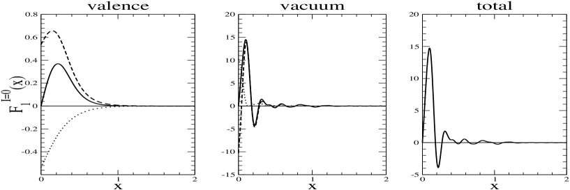
Figure 1: Isoscalar unpolarized structure function in the nucleon rest frame for a constituent quark mass of $400{\rm MeV}$. Dashed and dotted lines refer to the positive and negative frequency contributions, respectively.

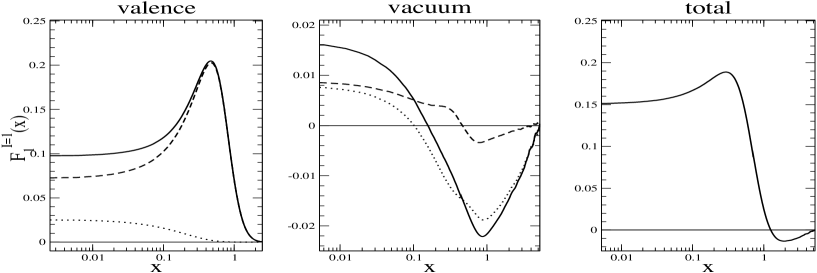
Figure 2: Isovector unpolarized structure function in the nucleon rest frame for a constituent quark mass of $400{\rm MeV}$. Note the logarithmic scale for the Bjorken variable. Dashed and dotted lines refer to the positive and negative frequency contributions, respectively.

For the vacuum contribution we find the unexpected result that it dominates the valence counterpart. Mainly this originates from the (additional) subtraction of the non-soliton piece mentioned after Eq. (44). Without that subtraction we would not get a finite result, of course. Neither would the momentum sum rule be fulfilled. However, this piece does not connect to the soliton rest frame and it is not clear at all whether or not transformation of the Bjorken variable should be performed before taking the difference between the soliton and non-soliton isoscalar unpolarized structure functions. Therefore we do not attach much relevance to this large vacuum contribution. As expected, the vacuum contribution is sub-dominant for the isovector unpolarized structure function.

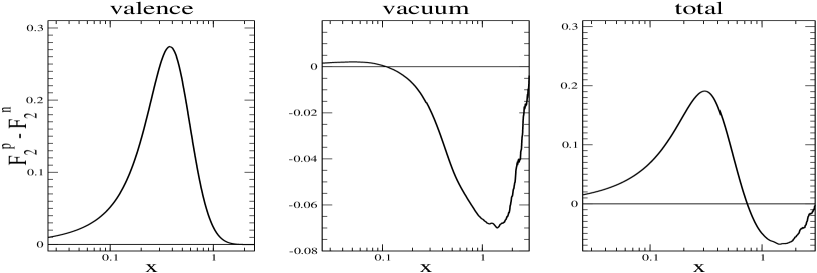
Figure 3: Unpolarized structure function $F_{2}^{p}(x)-F_{2}^{n}(x)$ in the nucleon rest frame for a constituent quark mass of $400{\rm MeV}$.

In Figure 3 we present the unpolarized structure function that enters the Gottfried sum rule, i.e. $F_{2}^{p}(x)-F_{2}^{n}(x)=2x\left[F_{1}^{p}(x)-F_{1}^{n}(x)\right]$ as the Callan-Gross relation holds in the soliton rest frame. The vacuum contribution turns slightly negative at large $x$ which persists when adding the dominating valence piece to form the total contribution of this structure function. In table 1 we compare our results for the Gottfried sum rule, $\mathcal{S}_{G}=\int_{0}^{\infty}\frac{dx}{x}\,\left(F_{2}^{p}-F_{2}^{n}\right)$, for various constituent quark masses to the experimental data from the NM Collaboration Arneodo et al. (1994). Under this integral, the vacuum part is even less significant as its positive and negative parts compensate. In total, the agreement for the Gottfried sum rule is surprisingly good since usually chiral soliton models reproduce empirical data with 30% accuracy Weigel (2008).

Table 1: The Gottfried sum rule for various values of $m$. The subscripts ’v’ and ’s’ denote the valence and vacuum contributions, respectively. The third column contains their sums.

$m\,[{\rm MeV}]$	$[\mathcal{S}_{G}]_{{\rm v}}$	$[\mathcal{S}_{G}]_{{\rm s}}$	$\mathcal{S}_{G}$	empirical value
$400$	$0.214$	$0.000156$	$0.214$
$450$	$0.225$	$0.000248$	$0.225$	$0.235\pm 0.026$ Arneodo et al. (1994)
$500$	$0.236$	$0.000356$	$0.237$

In Figures 4 and 5 we show the isoscalar and isovector contributions to the longitudinal polarized structure functions $\mathsf{g}^{I=0,1}_{1}$, respectively. In both pictures we display the valence and vacuum contributions as well as their sums. Also the positive and negative frequency components of the valence and vacuum parts are shown. Obviously these structure functions are indeed dominated by their valence contributions and we thus a posteriori verify the valence only approximation adopted in Ref. Weigel et al. (1997b). The only exception is the isoscalar structure function $\mathsf{g}_{2}$ for which the valence contribution is small by its own due to large cancellations in $\mathsf{g}_{2}=\mathsf{g}_{T}-\mathsf{g}_{1}$. We also recognize some minor oscillations in the vacuum contributions at larger $x$. These occur as remnants of numerical inaccuracies. We also remark that the present valence quark results do not exactly match those from Ref. Weigel et al. (1997b) in which a soliton profile from the proper-time regularization scheme was employed.

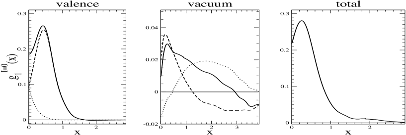
Figure 4: Isoscalar longitudinal polarized structure functions in the nucleon rest frame for a constituent quark mass of $400{\rm MeV}$. For the valence and vacuum contributions we separately display the positive (dashed) and negative (dotted) frequency contributions. The full lines are their sums. Note the small vertical scale for the vacuum contribution.

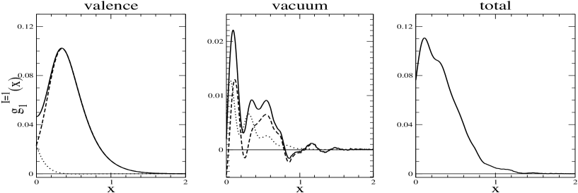
Figure 5: Same as Figure 4 for the isovector longitudinal polarized structure function.

We have computed the axial vector and singlet charges on one hand side via the respective sum rules, i.e. by integrating the structure functions $g^{I=1,0}_{1}(x)$ and on the other hand via the coordinate space matrix elements of $\tau_{3}\gamma_{3}\gamma_{5}$ and $\gamma_{3}\gamma_{5}$ as e.g. in Eqs. (72) and (73). The comparison in table 2 serves as test for the numerical accuracy which works perfectly in the vector case while some minor discrepancies are observed for the axial singlet charge. This is understood as the latter is actually quartic in the quark wave-functions (two of which are Fourier transformed) and it is also a double sum over those wave-functions. So even tiny numerical errors are amplified.

As is typical for chiral soliton models, the axial vector charge falls short off the measured datum by about 30-40% Weigel (2008). It has been argued that this could be remedied by $1/N_{C}$ corrections arising from a particular handling of the collective coordinate quantization Wakamatsu and Watabe (1993); Christov et al. (1994). However, these corrections do not emerge in the current approach and also lead to inconsistencies with PCAC Alkofer and Weigel (1993). On the other hand, the predicted axial singlet charge, which is linked to the proton spin problem Aidala et al. (2013), is well within the errors of the empirical value.

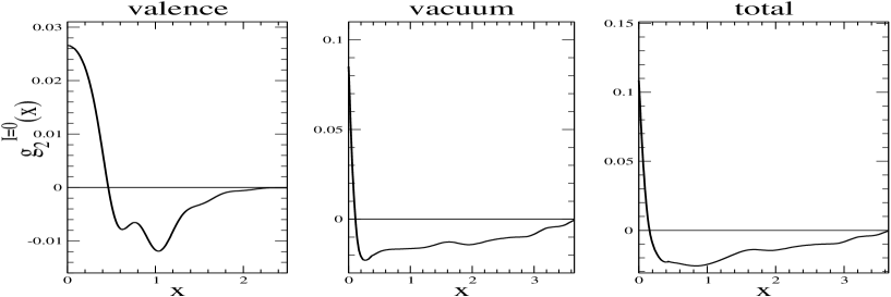
Figure 6: Isoscalar structure function, $\mathsf{g}_{2}$, in the nucleon rest frame for a constituent quark mass of $400{\rm MeV}$.

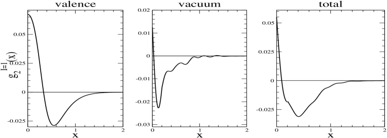
Figure 7: Isovector polarized structure functions, $\mathsf{g}_{2}$, in the nucleon rest frame for a constituent quark mass of $400{\rm MeV}$.

Table 2: The axial-vector and -singlet charges for various values of the constituent quark mass $m$. Subscripts are as in table 1. The data in parenthesis give the numerical results as obtained from the coordinate space representation.

$m\,[{\rm MeV}]$	$[g_{A}]_{{\rm v}}$	$[g_{A}]_{{\rm s}}$	$g_{A}$	empirical value
$400$	$0.734$	$0.065$	$0.799$ ($0.800$)
$450$	$0.715$	$0.051$	$0.766$ ($0.765$)	$1.2601\pm 0.0025$ Barnett et al. (1996)
$500$	$0.704$	$0.029$	$0.733$ ($0.733$)

$m\,[{\rm MeV}]$	$[g_{A}^{0}]_{{\rm v}}$	$[g_{A}^{0}]_{\rm s}$	$g_{A}^{0}$	empirical value
$400$	$0.344$	$0.0016$	$0.345$ ($0.350$)
$450$	$0.327$	$0.0021$	$0.329$ ($0.332$)	$0.33\pm 0.06$ Alexakhin et al. (2007)
$500$	$0.316$	$0.0028$	$0.318$ ($0.323$)

VII.2 Projection and evolution

The soliton picture for baryons employs a localized field configuration which generally breaks translational invariance. This causes the structure functions not to vanish when $x>1$ as would be demanded kinematically. This effect is obvious in the above figures. We note that it is not limited to soliton models but is observed, i.e. in the bag model as well Jaffe (1975). Using light cone coordinates in the bag model in one space dimension a mapping of the structure functions from the localized field configuration was constructed that annihilated the structure functions for $x>1$ Jaffe (1981). Guided by that construction a Lorentz boost was applied transforming the rest frame structure functions to the infinite momentum frame Gamberg et al. (1998)

$$f_{IMF}(x)=\frac{\Theta\left(1-x\right)}{1-x}f_{RF}\left(-\ln(1-x)\right)\,,$$ (74)

where $f_{RF}$ refers to any of the structure functions computed in Section VII.1. In what follows we will omit the label $IMF$ for the boosted structure functions.

Even though we have adopted the high energy Bjorken limit in our kinematical analysis of the Compton tensor, it must be emphasized that the NJL model is (at best) an approximation to QCD at the low mass scale, $\mu^{2}$ which is thus a hidden parameter in the approach. To compare with experimental data that are taken at higher energy scales, $Q_{\rm exp}^{2}$ we adopt Altarelli-Parisi (or DGLAP) equations Gribov and Lipatov (1972); Altarelli and Parisi (1977); Dokshitzer (1977), to evolve the model structure functions accordingly. To be precise, we integrate

$$f(x,t+\delta t)=f(x,t)+\delta t\frac{df(x,t)}{dt}\,.$$ (75)

with $\displaystyle t=\ln\left(\frac{Q^{2}}{\Lambda^{2}_{QCD}}\right)$ from $Q^{2}=\mu^{2}$ to $Q^{2}=Q_{\rm exp}^{2}$. The structure functions from Eq. (74) are the initial values and we tune $\mu^{2}$ for best fit at $Q_{\rm exp}^{2}$.

Since the isoscalar structure functions are associated with gluon type quantum numbers they mix under the evolution. We take this into account under the assumption that the gluon distributions vanish at $\mu^{2}$. We consider the leading order of the perturbative expansion sufficient to estimate the quality of our results. Then the evolution equations have the following structure

$$\frac{df^{(I=1)}(x,t)}{dt} =\frac{g_{QCD}(t)}{2\pi}C_{R}(F)\int_{x}^{1}\frac{dy}{y}P_{qq}(y)f^{(I=1)}\left(\frac{x}{y},t\right),$$ (76)

$$\frac{df^{(I=0)}(x,t)}{dt} =\frac{g_{QCD}(t)}{2\pi}C_{R}(F)\int_{x}^{1}\frac{dy}{y}\Biggl{\{}P_{qq}(y)f^{(I=0)}\left(\frac{x}{y},t\right)+P_{qg}(y)g\left(\frac{x}{y},t\right)\Biggr{\}},$$ (77)

$$\frac{dg(x,t)}{dt} =\frac{g_{QCD}(t)}{2\pi}C_{R}(F)\int_{x}^{1}\frac{dy}{y}\Biggl{\{}P_{gg}(y)g\left(\frac{x}{y},t\right)+P_{gq}(y)f^{(I=0)}\left(\frac{x}{y},t\right)\Biggr{\}}\,,$$ (78)

where $\displaystyle C_{R}(F)=\frac{\left(N_{f}^{2}-1\right)}{2N_{f}}$ is the color factor for $N_{f}$ flavors. Furthermore $\displaystyle g_{QCD}(t)=\frac{4\pi}{\beta_{0}t}$ with $\displaystyle\beta_{0}=\frac{11}{3}N_{C}-\frac{2}{3}N_{f}$ is the leading order perturbative running coupling constant. Explicit expressions for the splitting functions $P_{qq},\ldots,P_{gg}$, taken from Ref. Peskin and Schroeder (1995) are listed in Appendix D for completeness. From the evolved isoscalar and isovector components we finally obtain the proton and neutron structure functions as sum and difference

$$f^{(p,n)}(x,Q^{2})=\frac{1}{2}\left[f^{I=1}(x,Q^{2})\pm f^{I=0}(x,Q^{2})\right]\,.$$ (79)

We note that applying the perturbative QCD scheme to the model structure functions requires the identification of model and QCD degrees of freedom even though there is no definite reason for doing so other than the lack of any sensible alternative.

The second polarized structure function $\mathsf{g}_{2}$ contains subleading, twist three, elements that undergo a different evolution procedure that is also described in Appendix D.

VII.3 Comparison with experiment

As in previous calculations within the valence only approximation Weigel et al. (1997a, b); Weigel (2000) we take $\mu^{2}=0.4{\rm GeV^{2}}$ as initial value in the evolution differential equations. Smaller values contradict the perturbative nature of the evolution procedure as $\frac{g_{QCD}(t)}{2\pi}$ becomes sizable in view of $\Lambda_{QCD}^{2}=0.2{\rm GeV^{2}}$. On the other hand, significantly larger $\mu^{2}$ values worsen the agreement with experimental data.

         

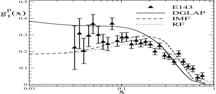
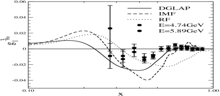
Figure 8: Model prediction for the longitudinal polarized proton structure functions. Left panel: $\mathsf{g}_{1}^{p}(x)$ ; right panel: $\mathsf{g}_{1}^{{}^{3}{\rm He}}(x)$. These functions are “DGLAP” evolved from $\mu^{2}=\mathrm{0.4\,GeV^{2}}$ to $Q^{2}=\mathrm{3\,GeV^{2}}$ after projected to the infinite momentum frame “IMF”. Data are from Refs. Abe et al. (1995, 1998) for the proton and from Ref. Flay et al. (2016) for helium. In the latter case $E$ refers to the electron energy.

In the left panel of Figure 8 we show the numerical result for the polarized proton structure function $\mathsf{g}_{1}$ obtained from the evolution equation at $Q^{2}=3{\rm GeV^{2}}$. We compare our results to experimental results from the E143 Collaboration Abe et al. (1995, 1998). At small $x$ the model results are somewhat larger than the data, but definitely the gross features are predominantly reproduced.

For the neutron data are available in terms of the helium structure function Flay et al. (2016)

$$\mathsf{g}_{1}^{{}^{3}{\rm He}}(x)\approx P_{n}\mathsf{g}_{1}^{n}(x)+P_{p}\mathsf{g}_{1}^{p}(x)-0.014\left[\mathsf{g}_{1}^{p}(x)-4\mathsf{g}_{1}^{n}(x)\right]\,,$$ (80)

with $P_{n}\approx 0.86$ and $P_{p}\approx-0.028$. From the right panel in Figure 8 we see that our model results reproduce the main features of the data: small positive values at large $x$ turning negative at moderate $x$, though the minimum is more pronounced by the model.

         

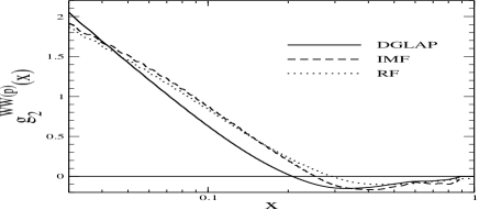
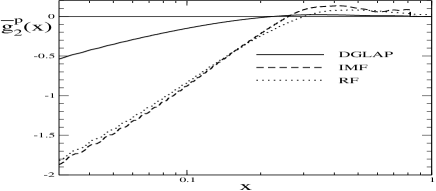
Figure 9: Model prediction for the polarized proton structure functions $\mathsf{g}_{2}^{WW(p)}(x)$ (left panel) and $\overline{\mathsf{g}}_{2}^{p}(x)$ (right panel) the are the twist-2 and -3 pieces of $\mathsf{g}_{2}$. These functions are “DGLAP” evolved from $\mu^{2}=\mathrm{0.4\,GeV^{2}}$ to $Q^{2}=\mathrm{5\,GeV^{2}}$ after projected to the infinite momentum frame “IMF”.

Next we discuss the results for the structure function $\mathsf{g}_{2}(x)$. As discussed in Appendix D the twist-2 and -3 pieces must be disentangled within the evolution whose result is shown in Figure 9. The effect of evolution is small for the twist-2 component but essential for the twist-3 counterpart.

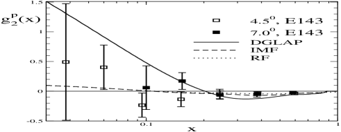
Figure 10: Model prediction for the polarized proton structure functions $\mathsf{g}_{2}^{p}(x)$. This function is “DGLAP” evolved from $\mu^{2}=\mathrm{0.4\,GeV^{2}}$ to $Q^{2}=\mathrm{5\,GeV^{2}}$ after projected to the infinite momentum frame “IMF”. Data is from Ref Abe et al. (1996).

When the end point of evolution is reached, the two components are combined to $\mathsf{g}_{2}^{p}(x,Q^{2})$. We display the model prediction in Figure 10 and see that the data are well produced. This shows that the higher twist contributions cannot be neglected. This suggests that the higher twist contributions cannot be neglected.

Recently data were reported for the neutron twist-3 moment

$$d_{2}^{n}(Q^{2})=3\int_{0}^{1}dx\,x^{2}\,\overline{\mathsf{g}}^{n}_{2}(x,Q^{2})$$ (81)

at two different transferred momenta: $d_{2}^{n}(3.21{\rm GeV}^{2})=-0.00421\pm 0.00114$ and $d_{2}^{n}(4.32{\rm GeV}^{2})=-0.00035\pm 0.00104$ Flay et al. (2016), where we added the listed errors in quadrature. For $m=400{\rm MeV}$ the model calculation yields $-0.00426$ and $-0.00409$, repsectively. While the lower $Q^{2}$ result nicely matches the observed value, the higher one differs by about three standard deviations. This discrepancy as a function of $Q^{2}$ indicates that the large $N_{C}$ approximation to evolve $\overline{\mathsf{g}}_{2}$ (cf. Appendix D) requires improvement.

Finally, in Figure 11 we display the unpolarized structure function that enters the Gottfried sum rule, i.e. $F_{2}^{p}(x)-F_{2}^{n}(x)$ using the evolution equation. Though the negative contribution from the Dirac vacuum (cf. Figure 2) around $x=1$ is tiny in the rest frame, it gets amplified when transforming to the infinite momentum frame by the factor $1/(1-x)$ in Eq. (74) thereby worsening the agreement with the experimental data collected by the NMC Arneodo et al. (1994).

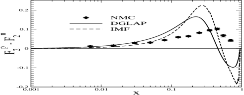
Figure 11: Model prediction for the unpolarized structure function that enters the Gottfried sum rule. This function is “DGLAP” evolved from $\mu^{2}=\mathrm{0.4\,GeV^{2}}$ to $Q^{2}=\mathrm{4\,GeV^{2}}$ after transformation to the infinite momentum frame “IMF”.

VIII Conclusion

We have presented the numerical simulation of nucleon structure functions within the NJL chiral soliton model. Central to this analysis has been the consistent implementation of the regularized vacuum contributions that arise from all quark spinors being distorted by the chiral soliton. Generally speaking, vacuum contributions should not be omitted in any quark model as no expansion scheme suppresses them. This is even more the case for the NJL model because the vacuum part significantly contributes to forming the soliton.

In our analysis we have only identified the symmetry currents of the model with those from QCD, not the quark distributions that are bilinear operators which are bilocal in the quark fields. Also, it is important to enforce the regularization on the action functional so that the regularization prescription for a given structure function is an unambiguous result. This increases the predictive power compared to previous similar studies that ”advocated” an ad hoc regularization of quark distributions Diakonov et al. (1997); Wakamatsu and Kubota (1998). A first principle regularization is particularly important when the sum rule for the structure function does not relate to coordinate space matrix elements of the quark fields. As an example we have seen that the isovector unpolarized structure functions are not subject to regularization (the explicit, lengthy formulas can be obtained from Ref. Takyi (2019)). The prediction for the corresponding, so-called Gottfried, sum rule decently matches the empirical value. This is a very favorable case for the valence only approximation as the vacuum contribution essentially integrates to zero due to an unexpected negative contribution at large $x$. For the isoscalar part we recognized that the subtraction of the zero-soliton vacuum contribution has a sizable effect at small $x$. The emergence of this contribution is somewhat surprising as it suggests that the zero-soliton vacuum has structure. Yet it is required for convergence as well as fulfilling the momentum sum rule. We emphasize that we observe acceptable agreement for polarized proton structure functions between our model results and the experimental data. For the polarized structure functions our numerically expensive computation indeed showed that the vacuum contribution is sub-dominant, except maybe for the isoscalar part of $\mathsf{g}_{2}$ where the valence part is tiny by itself. Nevertheless these results support the valence only approximation to a large extend.

In both, the unpolarized and polarized cases, the comparison with experiment required two additional operations on the model structure functions. As the soliton is a localized field configuration, translational invariance is lost and the rest frame structure functions must be Lorentz transformed to the infinite momentum frame. In turn the results from that transformation are subject to the perturbative QCD evolution scheme. This brings into the game the hidden parameter at which to commence the evolution. We took that to be the same as in the valence only approximation.

Even though we have separated positive and negative frequency contributions to the structure functions we stop short of identifying them as (anti-)quark distributions that parameterize semi-hard processes Gribov et al. (1983), like e.g. Drell-Yan Kenyon (1982). The reason being that we avoid to identify model and QCD quark degrees of freedom at the model scale. There are many other nucleon matrix elements of bilocal, bilinear quark operators for which experimental results or lattice data are available. Examples are chiral odd distributions Jaffe and Ji (1991a, 1992) or quasi-distributions Ji (2013); Alexandrou et al. (2017); Broniowski and Ruiz Arriola (2017). It is challenging to see whether quark distributions, or at least some of them, can also be formulated and computed with a first principle regularization scheme in the NJL chiral soliton model.

Appendix A Soliton matrix elements

The Dirac Hamiltonian $h$ of the hedgehog field configuration (21) commutes with the grand spin operator

$${\boldsymbol{G}}={\boldsymbol{J}}+\frac{{\boldsymbol{\tau}}}{2}={\boldsymbol{L}}+\frac{{\boldsymbol{\sigma}}}{2}+\frac{{\boldsymbol{\tau}}}{2},$$ (82)

which is the operator sum of the total spin ${\boldsymbol{J}}$ and the isospin ${\boldsymbol{\tau}}/2$. The total spin is the operator sum of the orbital angular momentum ${\boldsymbol{L}}$ and the intrinsic spin ${\boldsymbol{\sigma}}/2$. Since $h$ preserves ${\boldsymbol{G}}$, the eigenfunctions of the Dirac Hamiltonian are also eigenfunctions of ${\boldsymbol{G}}$. The quantum numbers of ${\boldsymbol{G}}$ are ${\boldsymbol{G}}^{2}=G(G+1)$ and $G_{3}=M$. The respective eigenfunctions are tensor spherical harmonics associated with the grand spin

$$\left[\mathcal{Y}_{LJGM}(\hat{{\boldsymbol{r}}})\right]_{si}=\sum_{m,s_{3},i_{3},J_{3}}C^{GM}_{JJ_{3},\frac{1}{2}i_{3}}C^{JJ_{3}}_{Lm,\frac{1}{2}s_{3}}\mathnormal{Y}_{Lm}(\hat{{\boldsymbol{r}}})\chi_{s}(s_{3})\chi_{i}(i_{3})$$ (83)

where $C^{GM}_{JJ_{3},\frac{1}{2}i_{3}}$ and $C^{JJ_{3}}_{Lm,\frac{1}{2}s_{3}}$ are $SU(2)$ Clebsch-Gordon coefficients that describe the coupling of $\chi_{s}$ and $\chi_{i}$, which are two components spinors and isospinors, respectively, and the spherical harmonic functions $Y_{Lm}$.

For a prescribed profile function $\Theta(r)$ the numerical diagonalization of the Dirac Hamiltonian (21) produces the radial functions $g_{\alpha}^{(G,\pm;i)}$ and $f_{\alpha}^{(G,\pm;i)}(i=1,2)$ that feature in eight component spinors Kahana and Ripka (1984)

$$\Psi_{\alpha}^{(G,+)}({\boldsymbol{r}})=\begin{pmatrix}{\rm i}g_{\alpha}^{(G,+;1)}(r)\mathcal{Y}_{GG+\frac{1}{2}GM}(\hat{{\boldsymbol{r}}})\\ f_{\alpha}^{(G,+;1)}(r)\mathcal{Y}_{G+1G+\frac{1}{2}GM}(\hat{{\boldsymbol{r}}})\end{pmatrix}+\begin{pmatrix}{\rm i}g_{\alpha}^{(G,+;2)}(r)\mathcal{Y}_{GG-\frac{1}{2}GM}(\hat{{\boldsymbol{r}}})\\ -f_{\alpha}^{(G,+;2)}(r)\mathcal{Y}_{G-1G-\frac{1}{2}GM}(\hat{{\boldsymbol{r}}})\end{pmatrix}$$ (84)

$$\Psi_{\alpha}^{(G,-)}({\boldsymbol{r}})=\begin{pmatrix}{\rm i}g_{\alpha}^{(G,-;1)}(r)\mathcal{Y}_{G+1G+\frac{1}{2}GM}(\hat{{\boldsymbol{r}}})\\ -f_{\alpha}^{(G,-;1)}(r)\mathcal{Y}_{GG+\frac{1}{2}GM}(\hat{{\boldsymbol{r}}})\end{pmatrix}+\begin{pmatrix}{\rm i}g_{\alpha}^{(G,-;2)}(r)\mathcal{Y}_{G-1G-\frac{1}{2}GM}(\hat{{\boldsymbol{r}}})\\ f_{\alpha}^{(G,-;2)}(r)\mathcal{Y}_{GG-\frac{1}{2}GM}(\hat{{\boldsymbol{r}}})\end{pmatrix}.$$ (85)

Here, the second superscript $(\pm)$ denotes the intrinsic parity defined by the parity eigenvalue as $(-1)^{G}\times(\pm 1)$. The radial functions are written as linear combinations of spherical Bessel functions that build the free spinors $\Psi_{\alpha}^{(0)}$. The order of these Bessel functions matches the angular momentum label (first subscript) of the multiplying $\mathcal{Y}$. The linear combination goes over momenta discretized by pertinent boundary conditions at a radius significantly larger than the extension of the profile function $\Theta(r)$. In Ref. Kahana and Ripka (1984) the condition that the radial function multiplying the $\mathcal{Y}$ with equal orbital angular momentum and grand spin indexes vanished at that large distance. In contrast, we impose that condition on the radial function of the upper component. This avoids spurious contributions to the moment of inertia Alkofer et al. (1996).

Writing

$${\rm e}^{{\rm i}{\boldsymbol{p}}\cdot{\boldsymbol{r}}}=4\pi\sum_{Lm}({\rm i})^{L}j_{L}(pr)\mathnormal{Y}_{Lm}^{*}(\hat{{\boldsymbol{r}}})\mathnormal{Y}_{Lm}(\hat{{\boldsymbol{p}}}).$$ (86)

we find the Fourier transform, Eq. (41) of the spinors

$$\widetilde{\Psi}_{\alpha}^{(G,+)}({\boldsymbol{p}})=({\rm i})^{G+1}\begin{pmatrix}\widetilde{g}_{\alpha}^{(G,+;1)}(p)\mathcal{Y}_{GG+\frac{1}{2}GM}(\hat{{\boldsymbol{p}}})\\ \widetilde{f}_{\alpha}^{(G,+;1)}(p)\mathcal{Y}_{G+1G+\frac{1}{2}GM}(\hat{{\boldsymbol{p}}})\end{pmatrix}+({\rm i})^{G+1}\begin{pmatrix}\widetilde{g}_{\alpha}^{(G,+;2)}(p)\mathcal{Y}_{GG-\frac{1}{2}GM}(\hat{{\boldsymbol{p}}})\\ \widetilde{f}_{\alpha}^{(G,+;2)}(p)\mathcal{Y}_{G-1G-\frac{1}{2}GM}(\hat{{\boldsymbol{p}}})\end{pmatrix}$$ (87)

$$\widetilde{\Psi}_{\alpha}^{(G,-)}({\boldsymbol{p}})=-({\rm i})^{G}\begin{pmatrix}\widetilde{g}_{\alpha}^{(G,-;1)}(p)\mathcal{Y}_{G+1G+\frac{1}{2}GM}(\hat{{\boldsymbol{p}}})\\ \widetilde{f}_{\alpha}^{(G,-;1)}(p)\mathcal{Y}_{GG+\frac{1}{2}GM}(\hat{{\boldsymbol{p}}})\end{pmatrix}+({\rm i})^{G}\begin{pmatrix}\widetilde{g}_{\alpha}^{(G,-;2)}(p)\mathcal{Y}_{G-1G-\frac{1}{2}GM}(\hat{{\boldsymbol{p}}})\\ ({\rm i})^{G}\widetilde{f}_{\alpha}^{(G,-;2)}(p)\mathcal{Y}_{GG-\frac{1}{2}GM}(\hat{{\boldsymbol{p}}})\end{pmatrix}\,.$$ (88)

The radial functions in momentum space are the Fourier-Bessel transforms

$$\widetilde{\phi}_{\alpha}(p)=\int_{0}^{\infty}dr\,r^{2}j_{L_{\alpha}}(pr)\phi_{\alpha}(r)\,,$$ (89)

where $L_{\alpha}$ is the angular momentum associated with the coordinate space radial wave-function $\phi_{\alpha}(r)$. Note that the grand spin spherical harmonic functions in momentum space are constructed precisely as in coordinate space, just that the argument is the momentum space solid angle. Note that the intrinsic parity is also conserved quantum number.

The valence quark carries $G=0$, then only the components with $J=+1/2$ are allowed for the eigenspinor

$$\Psi_{\alpha}^{0,+}({\boldsymbol{r}})=\Psi_{\rm v}({\boldsymbol{r}})=\begin{pmatrix}{\rm i}g_{\rm v}(r)\mathcal{Y}_{0,\frac{1}{2},0,0}(\hat{{\boldsymbol{r}}})\\ f_{\rm v}(r)\mathcal{Y}_{1,\frac{1}{2},0,0}(\hat{{\boldsymbol{r}}})\end{pmatrix}$$ (90)

here $g_{\rm v}(r)=g_{\alpha}^{(0,+;1)}(r)$ etc, are the particular eigenwave-functions. The cranking correction associated with the first order rotation (45) dwells in the channel with $G=1$ and negative intrinsic parity

$$\Psi_{\alpha}^{(1,-)}({\boldsymbol{r}})=\begin{pmatrix}{\rm i}g_{\alpha}^{(1)}(r)\mathcal{Y}_{2,\frac{3}{2},1,M}(\hat{{\boldsymbol{r}}})\\ -f_{\alpha}^{(1)}(r)\mathcal{Y}_{1,\frac{3}{2},1,M}(\hat{{\boldsymbol{r}}})\end{pmatrix}+\begin{pmatrix}{\rm i}g_{\alpha}^{(2)}(r)\mathcal{Y}_{0,\frac{1}{2},1,M}(\hat{{\boldsymbol{r}}})\\ f_{\alpha}^{(2)}(r)\mathcal{Y}_{1,\frac{1}{2},1,M}(\hat{{\boldsymbol{r}}})\end{pmatrix},$$ (91)

for convenience we have written $g_{\alpha}^{(1,-;1)}(r)$ as $g_{\alpha}^{(1)}(r)$ etc. Taking the Fourier transform of equation (45) gives

$$\widetilde{\psi}_{\rm v}({\boldsymbol{p}})=\widetilde{\Psi}_{\rm v}({\boldsymbol{p}})+\sum_{\alpha}\langle H_{\alpha}\rangle\widetilde{\Psi}_{\alpha}({\boldsymbol{p}}),$$ (92)

where

$$\widetilde{\Psi}_{\rm v}({\boldsymbol{p}})={\rm i}\begin{pmatrix}\widetilde{g}_{\rm v}(p)\mathcal{Y}_{0,\frac{1}{2},0,0}(\hat{{\boldsymbol{p}}})\\ \widetilde{f}_{\rm v}(p)\mathcal{Y}_{1,\frac{1}{2},0,0}(\hat{{\boldsymbol{p}}})\end{pmatrix}$$ (93)

and

$$\widetilde{\Psi}_{\alpha}({\boldsymbol{p}})=-{\rm i}\begin{pmatrix}\widetilde{g}_{\alpha}^{(1)}(p)\mathcal{Y}_{2,\frac{3}{2},1,M}(\hat{{\boldsymbol{p}}})-\widetilde{g}_{\alpha}^{(2)}(p)\mathcal{Y}_{0,\frac{1}{2},1,M}(\hat{{\boldsymbol{p}}})\\ \widetilde{f}_{\alpha}^{(1)}(p)\mathcal{Y}_{1,\frac{3}{2},1,M}(\hat{{\boldsymbol{p}}})-\widetilde{f}_{\alpha}^{(2)}(p)\mathcal{Y}_{1,\frac{1}{2},1,M}(\hat{{\boldsymbol{p}}})\end{pmatrix}.$$ (94)

The “matrix element” $\langle H_{\alpha}\rangle$ arises from perturbatively treating the collective rotation

$$\langle H_{\alpha}\rangle=\frac{1}{2}\frac{\langle\alpha|{\boldsymbol{\tau}}\cdot{\boldsymbol{\Omega}}|{\rm v}\rangle}{\epsilon_{\rm v}-\epsilon_{\alpha}}.$$ (95)

Appendix B Unpolarized Structure Functions at Leading Order

The level sums (over $\alpha$) as e.g. in Eq. (42) concern the label of the radial function, grand spin ($G$) and its projection ($M$). As we average of the direction of the virtual photon Diakonov et al. (1997), the matrix elements are degenerate in $M$. This produces the extra factor $2G+1$ that we make explicit.

It is then straightforward to compute the matrix elements that appear in (38):

$$\int d\Omega_{p}\widetilde{\Psi}_{\alpha}^{\dagger}({\boldsymbol{p}})\widetilde{\Psi}_{\alpha}({\boldsymbol{p}})\quad\text{and}$$ (96)

$$\int d\Omega_{p}\widetilde{\Psi}_{\alpha}^{\dagger}({\boldsymbol{p}})\hat{{\boldsymbol{p}}}\cdot{\boldsymbol{\alpha}}\widetilde{\Psi}_{\alpha}({\boldsymbol{p}})=\int d\Omega_{p}\widetilde{\Psi}_{\alpha}^{\dagger}({\boldsymbol{p}})\hat{{\boldsymbol{p}}}\cdot{\boldsymbol{\sigma}}\gamma_{5}\widetilde{\Psi}_{\alpha}({\boldsymbol{p}}).$$ (97)

The positive intrinsic parity of the matrix element of (96) is obtained as

$$\int d\Omega_{p}\widetilde{\Psi}_{\alpha}^{\dagger(G,+)}({\boldsymbol{p}})\widetilde{\Psi}_{\alpha}^{(G,+)}({\boldsymbol{p}})=(2G+1)\Bigl{(}\widetilde{g}_{\alpha}^{(G,+;1)}(p)^{2}+\widetilde{f}_{\alpha}^{(G,+;1)}(p)^{2}+\widetilde{g}_{\alpha}^{(G,+;2)}(p)^{2}+\widetilde{f}_{\alpha}^{(G,+;2)}(p)^{2}\Bigr{)},$$ (98)

and for the negative intrinsic parity as

$$\int d\Omega_{p}\widetilde{\Psi}_{\alpha}^{\dagger(G,-)}({\boldsymbol{p}})\widetilde{\Psi}_{\alpha}^{(G,-)}({\boldsymbol{p}})=(2G+1)\Bigl{(}\widetilde{g}_{\alpha}^{(G,-;1)}(p)^{2}+\widetilde{f}_{\alpha}^{(G,-;1)}(p)^{2}+\widetilde{g}_{\alpha}^{(G,-;2)}(p)^{2}+\widetilde{f}_{\alpha}^{(G,-;2)}(p)^{2}\Bigr{)}.$$ (99)

Here the overall factor $(2G+1)$ arises from summing the grand spin projection contained in $\sum_{\alpha}$.

Table 3: Matrix elements $\int d\Omega_{p}\mathcal{Y}_{L^{\prime}J^{\prime}GM}({\boldsymbol{p}})\hat{{\boldsymbol{p}}}\cdot{\boldsymbol{\sigma}}\mathcal{Y}_{LJGM}({\boldsymbol{p}})$.

$J^{\prime}=G-\frac{1}{2}$		$J^{\prime}=G+\frac{1}{2}$
$L^{\prime}=G-1$	$L^{\prime}=G$	$L^{\prime}=G$	$L^{\prime}=G+1$
$0$	$-1$	$0$	$0$	$L=G-1$
					$J=G-\frac{1}{2}$
$-1$	$0$	$0$	$0$	$L=G$
$0$	$0$	$0$	$-1$	$L=G$
					$J=G+\frac{1}{2}$
$0$	$0$	$-1$	$0$	$L=G+1$

From Table (3) the positive intrinsic parity of the matrix element of (97) is obtained as

$$\int d\Omega_{p}\,\widetilde{\Psi}_{\alpha}^{\dagger(G,+)}({\boldsymbol{p}})\hat{{\boldsymbol{p}}}\cdot{\boldsymbol{\sigma}}\gamma_{5}\widetilde{\Psi}_{\alpha}^{(G,+)}({\boldsymbol{p}})=-2(2G+1)\Bigl{(}\widetilde{g}_{\alpha}^{(G,+;1)}(p)\widetilde{f}_{\alpha}^{(G,+;1)}(p)+\widetilde{g}_{\alpha}^{(G,+;2)}(p)\widetilde{f}_{\alpha}^{(G,+;2)}(p)\Bigr{)},$$ (100)

and that for the negative intrinsic parity as

$$\int d\Omega_{p}\,\widetilde{\Psi}_{\alpha}^{\dagger(G,-)}({\boldsymbol{p}})\hat{{\boldsymbol{p}}}\cdot{\boldsymbol{\sigma}}\gamma_{5}\widetilde{\Psi}_{\alpha}^{(G,-)}({\boldsymbol{p}})=-2(2G+1)\Bigl{(}\widetilde{g}_{\alpha}^{(G,-;1)}(p)\widetilde{f}_{\alpha}^{(G,-;1)}(p)+\widetilde{g}_{\alpha}^{(G,-;2)}(p)\widetilde{f}_{\alpha}^{(G,-;2)}(p)\Bigr{)}.$$

The matrix element from the valence contribution (46) is easily obtained, using the definition of the decomposition of the valence wave function (93). They are given as

$$\int d\Omega_{p}\widetilde{\Psi}_{\rm v}^{\dagger}({\boldsymbol{p}})\widetilde{\Psi}_{\rm v}({\boldsymbol{p}})=\widetilde{g}_{\rm v}(p)^{2}+\widetilde{f}_{\rm v}(p)^{2}\quad\text{and}$$ (101)

$$\int d\Omega_{p}\widetilde{\Psi}_{\rm v}^{\dagger}({\boldsymbol{p}})\hat{{\boldsymbol{p}}}\cdot{\boldsymbol{\sigma}}\gamma_{5}\widetilde{\Psi}_{\rm v}({\boldsymbol{p}})=-2\widetilde{g}_{\rm v}(p)\widetilde{f}_{\rm v}(p)$$ (102)

at leading order $1/N_{C}$.

Appendix C Polarized Structure Functions at Leading Order

Here we list the matrix elements that appear in the vacuum contribution of the polarized structure functions, Eqs. (48) and (50). The matrix element to be considered are

$$\int d\Omega_{p}\widetilde{\Psi}_{\alpha}^{\dagger}({\boldsymbol{p}})\hat{{\boldsymbol{p}}}\cdot{\boldsymbol{\tau}}\gamma_{5}\widetilde{\Psi}_{\alpha}({\boldsymbol{p}}),$$ (103)

$$\int d\Omega_{p}\widetilde{\Psi}_{\alpha}^{\dagger}({\boldsymbol{p}})\hat{{\boldsymbol{p}}}\cdot{\boldsymbol{\tau}}\hat{{\boldsymbol{p}}}\cdot{\boldsymbol{\sigma}}\widetilde{\Psi}_{\alpha}({\boldsymbol{p}})\quad\text{and}$$ (104)

$$\int d\Omega_{p}\widetilde{\Psi}_{\alpha}^{\dagger}({\boldsymbol{p}}){\boldsymbol{\tau}}\cdot{\boldsymbol{\sigma}}\widetilde{\Psi}_{\alpha}({\boldsymbol{p}}).$$ (105)

Table 4: Matrix elements $\int d\Omega_{p}\mathcal{Y}_{L^{\prime}J^{\prime}GM}({\boldsymbol{p}})\hat{{\boldsymbol{p}}}\cdot{\boldsymbol{\tau}}\mathcal{Y}_{LJGM}({\boldsymbol{p}})$. The overall factor $1/(2G+1)$

needs to be multiplied. $J^{\prime}=G-\frac{1}{2}$ $J^{\prime}=G+\frac{1}{2}$ $L^{\prime}=G-1$ $L^{\prime}=G$ $L^{\prime}=G$ $L^{\prime}=G+1$ $0$ $-1$ $-2\sqrt{G(G+1)}$ $0$ $L=G-1$ $J=G-\frac{1}{2}$ $-1$ $0$ $0$ $-2\sqrt{G(G+1)}$ $L=G$ $-2\sqrt{G(G+1)}$ $0$ $0$ $1$ $L=G$ $J=G+\frac{1}{2}$ $0$ $-2\sqrt{G(G+1)}$ $1$ $0$ $L=G+1$

The matrix element (103) is computed from the matrix elements from Table 4: the positive intrinsic parity is obtained as

$$\int d\Omega_{p}\,\widetilde{\Psi}_{\alpha}^{\dagger(G,+)}({\boldsymbol{p}})\hat{{\boldsymbol{p}}}\cdot{\boldsymbol{\tau}}\gamma_{5}\widetilde{\Psi}_{\alpha}^{(G,+)}({\boldsymbol{p}}) =2\left(\widetilde{g}_{\alpha}^{(G,+;1)}(p)\widetilde{f}_{\alpha}^{(G,+;1)}(p)-\widetilde{g}_{\alpha}^{(G,+;2)}(p)\widetilde{f}_{\alpha}^{(G,+;2)}(p)\right)$$ (106)

$$-4\sqrt{G(G+1)}\Bigl{(}\widetilde{g}_{\alpha}^{(G,+;1)}(p)\widetilde{f}_{\alpha}^{(G,+;2)}(p)+\widetilde{g}_{\alpha}^{(G,+;2)}(p)\widetilde{f}_{\alpha}^{(G,+;1)}(p)\Bigr{)}\,,$$ (107)

and that for negative intrinsic parity as

$$\int d\Omega_{p}\,\widetilde{\Psi}_{\alpha}^{\dagger(G,-)}({\boldsymbol{p}})\hat{{\boldsymbol{p}}}\cdot{\boldsymbol{\tau}}\gamma_{5}\widetilde{\Psi}_{\alpha}^{(G,-)}({\boldsymbol{p}}) =2\left(\widetilde{g}_{\alpha}^{(G,-;1)}(p)\widetilde{f}_{\alpha}^{(G,-;1)}(p)-\widetilde{g}_{\alpha}^{(G,-;2)}(p)\widetilde{f}_{\alpha}^{(G,-;2)}(p)\right)$$ (108)

$$+4\sqrt{G(G+1)}\Bigl{(}\widetilde{g}_{\alpha}^{(G,-;1)}(p)\widetilde{f}_{\alpha}^{(G,-;2)}(p)+\widetilde{g}_{\alpha}^{(G,-;2)}(p)\widetilde{f}_{\alpha}^{(G,-;1)}(p)\Bigr{)}\,.$$ (109)

Also the matrix element (104) is computed from the matrix elements from Table 5:

Table 5: Matrix elements $\int d\Omega_{p}\mathcal{Y}_{L^{\prime}J^{\prime}GM}({\boldsymbol{p}})\hat{{\boldsymbol{p}}}\cdot{\boldsymbol{\tau}}\hat{{\boldsymbol{p}}}\cdot{\boldsymbol{\sigma}}\mathcal{Y}_{LJGM}({\boldsymbol{p}})$. The overall factor $1/(2G+1)$

needs to be multiplied. $J^{\prime}=G-\frac{1}{2}$ $J^{\prime}=G+\frac{1}{2}$ $L^{\prime}=G-1$ $L^{\prime}=G$ $L^{\prime}=G$ $L^{\prime}=G+1$ $1$ $0$ $0$ $2\sqrt{G(G+1)}$ $L=G-1$ $J=G-\frac{1}{2}$ $0$ $1$ $2\sqrt{G(G+1)}$ $0$ $L=G$ $0$ $2\sqrt{G(G+1)}$ $-1$ $0$ $L=G$ $J=G+\frac{1}{2}$ $2\sqrt{G(G+1)}$ $0$ $0$ $-1$ $L=G+1$

the positive intrinsic parity contribution is given as

$$\int d\Omega_{p}\,\widetilde{\Psi}_{\alpha}^{\dagger(G,+)}({\boldsymbol{p}})\hat{{\boldsymbol{p}}}\cdot{\boldsymbol{\tau}}\hat{{\boldsymbol{p}}}\cdot{\boldsymbol{\sigma}}\widetilde{\Psi}_{\alpha}^{(G,+)}({\boldsymbol{p}}) =\Bigl{(}-\widetilde{g}_{\alpha}^{(G,+;1)}(p)^{2}-\widetilde{f}_{\alpha}^{(G,+;1)}(p)^{2}+\widetilde{g}_{\alpha}^{(G,+;2)}(p)^{2}+\widetilde{f}_{\alpha}^{(G,+;2)}(p)^{2}\Bigr{)}$$ (110)

$$+4\sqrt{G(G+1)}\Bigl{(}\widetilde{g}_{\alpha}^{(G,+;1)}(p)\widetilde{g}_{\alpha}^{(G,+;2)}(p)+\widetilde{f}_{\alpha}^{(G,+;1)}(p)\widetilde{f}_{\alpha}^{(G,+;2)}(p)\Bigr{)},$$ (111)

and that for the negative intrinsic parity as

$$\int d\Omega_{p}\,\widetilde{\Psi}_{\alpha}^{\dagger(G,-)}({\boldsymbol{p}})\hat{{\boldsymbol{p}}}\cdot{\boldsymbol{\tau}}\hat{{\boldsymbol{p}}}\cdot{\boldsymbol{\sigma}}\widetilde{\Psi}_{\alpha}^{(G,-)}({\boldsymbol{p}}) =\Bigl{(}-\widetilde{g}_{\alpha}^{(G,-;1)}(p)^{2}-\widetilde{f}_{\alpha}^{(G,-;1)}(p)^{2}+\widetilde{g}_{\alpha}^{(G,-;2)}(p)^{2}+\widetilde{f}_{\alpha}^{(G,-;2)}(p)^{2}\Bigr{)}$$ (112)

$$-4\sqrt{G(G+1)}\Bigl{(}\widetilde{g}_{\alpha}^{(G,-;1)}(p)\widetilde{g}_{\alpha}^{(G,-;2)}(p)+\widetilde{f}_{\alpha}^{(G,-;1)}(p)\widetilde{f}_{\alpha}^{(G,-;2)}(p)\Bigr{)}.$$ (113)

Furthermore the matrix element (105) is computed from the matrix elements from Table 6:

Table 6: Matrix elements $\int d\Omega_{p}\mathcal{Y}_{L^{\prime}J^{\prime}GM}({\boldsymbol{p}}){\boldsymbol{\tau}}\cdot{\boldsymbol{\sigma}}\mathcal{Y}_{LJGM}({\boldsymbol{p}})$. The overall factor $1/(2G+1)$

needs to be multiplied. $J^{\prime}=G-\frac{1}{2}$ $J^{\prime}=G+\frac{1}{2}$ $L^{\prime}=G-1$ $L^{\prime}=G$ $L^{\prime}=G$ $L^{\prime}=G+1$ $2G+1$ $0$ $0$ $0$ $L=G-1$ $J=G-\frac{1}{2}$ $0$ $-(2G-1)$ $4\sqrt{G(G+1)}$ $0$ $L=G$ $0$ $4\sqrt{G(G+1)}$ $-(2G+3)$ $0$ $L=G$ $J=G+\frac{1}{2}$ $0$ $0$ $0$ $2G+1$ $L=G+1$

the positive intrinsic parity contribution becomes

$$\int d\Omega_{p}\,\widetilde{\Psi}_{\alpha}^{\dagger(G,+)}({\boldsymbol{p}}){\boldsymbol{\tau}}\cdot{\boldsymbol{\sigma}}\widetilde{\Psi}_{\alpha}^{(G,+)}({\boldsymbol{p}}) =(2G+1)\left(\widetilde{f}_{\alpha}^{(G,+;1)}(p)^{2}+\widetilde{f}_{\alpha}^{(G,+;2)}(p)^{2}\right)-(2G+3)\widetilde{g}_{\alpha}^{(G,+;1)}(p)^{2}$$ (114)

$$+(2G-1)\widetilde{g}_{\alpha}^{(G,+;2)}(p)^{2}+8\sqrt{G(G+1)}\widetilde{g}_{\alpha}^{(G,+;1)}(p)\widetilde{g}_{\alpha}^{(G,+;2)}(p)\,,$$ (115)

and for negative intrinsic parity becomes

$$\int d\Omega_{p}\,\widetilde{\Psi}_{\alpha}^{\dagger(G,-)}({\boldsymbol{p}}){\boldsymbol{\tau}}\cdot{\boldsymbol{\sigma}}\widetilde{\Psi}_{\alpha}^{(G,-)}({\boldsymbol{p}}) =(2G+1)\left(\widetilde{g}_{\alpha}^{(G,-;1)}(p)^{2}+\widetilde{g}_{\alpha}^{(G,-;2)}(p)^{2}\right)-(2G+3)\widetilde{f}_{\alpha}^{(G,-;1)}(p)^{2}$$ (116)

$$-(2G-1)\widetilde{f}_{\alpha}^{(G,-;2)}(p)^{2}-8\sqrt{G(G+1)}\widetilde{f}_{\alpha}^{(G,-;1)}(p)\widetilde{f}_{\alpha}^{(G,-;2)}(p)\,.$$ (117)

Appendix D Splitting functions

Here we list the splitting functions used in Eqs. (76), (77) and (78). They are different for the isovector, isosinglet and gluon contributions and are given as Altarelli and Parisi (1977); Altarelli et al. (1994)

$$P_{qq}(z) =\frac{1+z^{2}}{\left(1-z\right)_{+}},$$ (118)

$$P_{qg}(z) =\frac{1}{2C_{R}(F)}\left[z^{2}+(1-z)^{2}\right],$$ (119)

$$P_{gq}(z) =\frac{1+(1-z)^{2}}{z},$$ (120)

$$P_{gg}(z) =2\Big{[}\frac{1-z}{z}+\frac{z}{(1-z)_{+}}+z(1-z)\Big{]}.$$ (121)

They determine the probability for the parton $m$ to emit a parton $n$ such that the momentum of the parton $m$ is reduced by the fraction $z$. The regularized function $(1-z)^{-1}_{+}$ is defined under the integral by Altarelli and Parisi (1977)

$$\int_{0}^{1}dz\,\frac{f(z)}{\left(1-z\right)_{+}}=\int_{0}^{1}dz\,\frac{f(z)-f(1)}{1-z}.$$ (122)

In the above $\displaystyle C_{R}(F)=\frac{\left(N_{f}^{2}-1\right)}{2N_{f}}$ is the color factor for $N_{f}$ flavors. Also the running coupling constant in the leading order is given by $\displaystyle g_{QCD}(t)=\frac{4\pi}{\beta_{0}t}$ with $\displaystyle\beta_{0}=\frac{11}{3}N_{c}-\frac{2}{3}N_{f}$ being the coefficient of the leading term of the QCD $\beta$-function. Using the “$+$ ” prescription, the evolution equations for the isovector, isosinglet and gluon contributions become Altarelli et al. (1994)

$$\frac{df^{(I=1)}(x,t)}{dt} =\frac{2C_{R}(F)}{9t}\Bigg{\{}\int_{x}^{1}\frac{dy}{y}\left(\frac{1+y^{2}}{1-y}\right)\Bigg{[}\frac{1}{y}f^{(I=1)}\left(\frac{x}{y},t\right)-f^{(I=1)}(x,t)\Bigg{]}$$ (123)

$$+\Bigg{[}x+\frac{x^{2}}{2}+2\ln\left(1-x\right)\Bigg{]}f^{(I=1)}(x,t)\Bigg{\}},$$ (124)

$$\frac{df^{(I=0)}(x,t)}{dt} =\frac{2C_{R}(F)}{9t}\Bigg{\{}\int_{x}^{1}\frac{dy}{y}\Bigg{(}\left(\frac{1+y^{2}}{1-y}\right)\Bigg{[}\frac{1}{y}f^{(I=0)}\left(\frac{x}{y},t\right)-f^{(I=0)}(x,t)\Bigg{]}$$ (125)

$$+\frac{3}{4}\left(y^{2}+(1-y^{2})\right)\frac{g(x,t)}{y}\Bigg{)}+\Bigg{[}x+\frac{x^{2}}{2}+2\ln\left(1-x\right)\Bigg{]}f^{I=0}(x,t)\Bigg{\}},$$ (126)

$$\frac{dg(x,t)}{dt} =\frac{2C_{R}(F)}{9t}\Bigg{\{}\int_{x}^{1}\frac{dy}{y}\Bigg{(}\left(\frac{1+(1-y)^{2}}{y}\right)f^{(I=0)}\left(\frac{x}{y},t\right)$$ (127)

$$+\frac{9}{2}\left(\frac{1-y}{y}+y^{2}(1-y)\right)\frac{g\left(\frac{x}{y},t\right)}{y}+\frac{9}{2}\frac{g\left(\frac{x}{y},t\right)-g(x,t)}{1-y}\Bigg{)}+\Bigg{[}\frac{3}{2}+\frac{9}{2}\ln\left(1-x\right)\Bigg{]}g(x,t)\Bigg{\}}.$$ (128)

Now, since our NJL model calculations do not account for any gluon content in the nucleon, we assume in our numerical calculations that, at the initial boundary scale $\mu^{2}$, the gluon content, $f(x,t_{0})=0$ for both the polarized and unpolarized structure functions.

Unlike the polarized spin structure function $\mathsf{g}_{1}(x)$ of the nucleon and the unpolarized structure functions, the nucleon’s second polarized spin structure function $\mathsf{g}_{2}$ involves contributions from quark-gluon iterations and quark masses Jaffe (1990); Ji and Chou (1990); Jaffe and Ji (1991b). According to the standard operator product expansion analysis, these contributions come from the twist-3 local operators. It, however, also receives contribution from twist-2 local operators under the impulse approximation. Thus, the structure function $\mathsf{g}_{2}$ can be written as the sum of the twist pieces

$$\mathsf{g}_{2}(x,Q^{2})=\mathsf{g}_{2}^{WW}(x,Q^{2})+\overline{\mathsf{g}}_{2}(x,Q^{2}),$$ (129)

where the twist-2 piece is given as Wandzura and Wilczek (1977)

$$\mathsf{g}_{2}^{WW}(x,Q^{2})=-\mathsf{g}_{1}(x,Q^{2})+\int_{0}^{1}\frac{1}{y}\mathsf{g}_{1}(y,Q^{2})\mathrm{d}y\,,$$ (130)

while that of the twist-3 piece is

$$\overline{\mathsf{g}}_{2}(x,Q^{2})=\mathsf{g}_{1}(x,Q^{2})+\mathsf{g}_{2}(x,Q^{2})-\int_{0}^{1}\frac{1}{y}\mathsf{g}_{1}(y,Q^{2})\mathrm{d}y\,.$$ (131)

The twist-2 part undergoes the ordinary evolution as in Eq. (128) and the twist-3 piece is first parameterized by its moments

$$M_{j}(\mu^{2})=\int dx\,x^{j-1}\overline{\mathsf{g}}_{2}(x,\mu^{2})$$ (132)

that scale as Jaffe (1990)

$$M_{j}(Q^{2})=\left[\frac{\ln(\mu^{2})}{\ln(Q^{2})}\right]^{\frac{\gamma_{j-1}}{\beta_{0}}}\qquad{\rm with}\qquad\gamma_{j-1}=2N_{c}\left[\psi(j)+\frac{1}{2j}+\gamma_{E}-\frac{1}{4}\right]\,.$$ (133)

Here $\psi(j)$ is the logarithmic derivative of the $\Gamma$-function. Then $\overline{\mathsf{g}}_{2}(x,Q^{2})$ is obtained by expressing it in terms of the evolved moments, i.e. by inverting Eq. (132).

References

• Muta (1987) T. Muta, Foundations of Quantum Chromodynamics (World Scientific, Singapore, 1987).
• Roberts (1990) R. G. Roberts, The Structure of the Proton (Cambridge Monographs on Mathematical Physics, 1990).
• Ynduráin (1993) F. J. Ynduráin, The Theory of Quark and Gluon Interactions (Springer-Verlag, Berlin - Heidelberg - New York, 1993).
• Pumplin et al. (2002) J. Pumplin, D. R. Stump, J. Huston, H. L. Lai, P. M. Nadolsky, and W. K. Tung, JHEP 07, 012 (2002), eprint hep-ph/0201195.
• Kokkedee (1979) J. J. J. Kokkedee, The Quark Model (Benjamin, New York, 1979).
• Thomas (1984) A. W. Thomas, Adv. Nucl. Phys. 13, 1 (1984).
• Maris and Roberts (2003) P. Maris and C. D. Roberts, Int. J. Mod. Phys. E12, 297 (2003), eprint nucl-th/0301049.
• Weigel (2008) H. Weigel, Lect. Notes Phys. 743, 1 (2008).
• Alkofer et al. (1996) R. Alkofer, H. Reinhardt, and H. Weigel, Phys. Rept. 265, 139 (1996), eprint hep-ph/9501213.
• Christov et al. (1996) C. Christov, A. Blotz, H.-C. Kim, P. Pobylitsa, T. Watabe, T. Meissner, E. Ruiz Arriola, and K. Goeke, Prog. Part. Nucl. Phys. 37, 91 (1996), eprint hep-ph/9604441.
• Weigel et al. (1997a) H. Weigel, L. P. Gamberg, and H. Reinhardt, Phys. Lett. B399, 287 (1997a), eprint hep-ph/9604295.
• Weigel et al. (1997b) H. Weigel, L. P. Gamberg, and H. Reinhardt, Phys. Rev. D55, 6910 (1997b), eprint hep-ph/9609226.
• Diakonov et al. (1996) D. Diakonov, V. Petrov, P. Pobylitsa, M. V. Polyakov, and C. Weiss, Nucl. Phys. B480, 341 (1996), eprint hep-ph/9606314.
• Diakonov et al. (1997) D. Diakonov, V. Yu. Petrov, P. V. Pobylitsa, M. V. Polyakov, and C. Weiss, Phys. Rev. D56, 4069 (1997), eprint hep-ph/9703420.
• Pobylitsa et al. (1999) P. V. Pobylitsa, M. V. Polyakov, K. Goeke, T. Watabe, and C. Weiss, Phys. Rev. D59, 034024 (1999), eprint hep-ph/9804436.
• Wakamatsu and Kubota (1998) M. Wakamatsu and T. Kubota, Phys. Rev. D57, 5755 (1998), eprint hep-ph/9707500.
• Wakamatsu and Kubota (1999) M. Wakamatsu and T. Kubota, Phys. Rev. D60, 034020 (1999), eprint hep-ph/9809443.
• Wakamatsu (2003a) M. Wakamatsu, Phys. Rev. D67, 034005 (2003a).
• Wakamatsu (2003b) M. Wakamatsu, Phys. Rev. D67, 034006 (2003b), eprint hep-ph/0212356.
• Weigel et al. (1999) H. Weigel, E. Ruiz Arriola, and L. P. Gamberg, Nucl. Phys. B560, 383 (1999), eprint hep-ph/9905329.
• Takyi and Weigel (2019) I. Takyi and H. Weigel (2019), Contribution to the Proc. of Int. Conf. Quarks and Nuclear Physics, Tsukuba, Japan, Nov. 2018, eprint 1903.10748.
• Frederico and Miller (1994) T. Frederico and G. A. Miller, Phys. Rev. D50, 210 (1994).
• Davidson and Ruiz Arriola (1995) R. M. Davidson and E. Ruiz Arriola, Phys. Lett. B348, 163 (1995).
• Reinhardt (1989) H. Reinhardt, Nucl. Phys. A503, 825 (1989).
• Adkins et al. (1983) G. S. Adkins, C. R. Nappi, and E. Witten, Nucl. Phys. B228, 552 (1983).
• Kahana and Ripka (1984) S. Kahana and G. Ripka, Nucl. Phys. A429, 462 (1984).
• Takyi (2019) I. Takyi, Ph.D. thesis, Stellenbosch University (2019), to be published on SUNScholar: scholar.sun.ac.za.
• Bjorken (1970) J. D. Bjorken, Phys. Rev. D1, 1376 (1970).
• Adler (1966) S. L. Adler, Phys. Rev. 143, 1144 (1966).
• Weigel et al. (1996) H. Weigel, L. P. Gamberg, and H. Reinhardt, Mod. Phys. Lett. A11, 3021 (1996).
• Gamberg et al. (1998) L. P. Gamberg, H. Reinhardt, and H. Weigel, Int. J. Mod. Phys. A13, 5519 (1998), eprint hep-ph/9707352.
• Arneodo et al. (1994) M. Arneodo et al. (New Muon), Phys. Rev. D50, R1 (1994).
• Wakamatsu and Watabe (1993) M. Wakamatsu and T. Watabe, Phys. Lett. B312, 184 (1993).
• Christov et al. (1994) C. V. Christov, A. Blotz, K. Goeke, P. Pobylitsa, V. Petrov, M. Wakamatsu, and T. Watabe, Phys. Lett. B325, 467 (1994), eprint hep-ph/9312279.
• Alkofer and Weigel (1993) R. Alkofer and H. Weigel, Phys. Lett. B319, 1 (1993), eprint hep-ph/9308327.
• Aidala et al. (2013) C. A. Aidala, S. D. Bass, D. Hasch, and G. K. Mallot, Rev. Mod. Phys. 85, 655 (2013), eprint 1209.2803.
• Barnett et al. (1996) R. M. Barnett et al. (Particle Data Group), Phys. Rev. D54, 1 (1996).
• Alexakhin et al. (2007) V. Yu. Alexakhin et al. (COMPASS), Phys. Lett. B647, 8 (2007), eprint hep-ex/0609038.
• Jaffe (1975) R. L. Jaffe, Phys. Rev. D11, 1953 (1975).
• Jaffe (1981) R. L. Jaffe, Annals Phys. 132, 32 (1981).
• Gribov and Lipatov (1972) V. N. Gribov and L. N. Lipatov, Sov. J. Nucl. Phys. 15, 438 (1972), [Yad. Fiz.15,781(1972)].
• Altarelli and Parisi (1977) G. Altarelli and G. Parisi, Nucl. Phys. B126, 298 (1977).
• Dokshitzer (1977) Y. L. Dokshitzer, Sov. Phys. JETP 46, 641 (1977), [Zh. Eksp. Teor. Fiz.73,1216(1977)].
• Peskin and Schroeder (1995) M. E. Peskin and D. V. Schroeder, An Introduction to Quantum Field Theory (Westview Press, 1995).
• Weigel (2000) H. Weigel, Nucl. Phys. A670, 92 (2000), eprint hep-ph/9902390.
• Abe et al. (1995) K. Abe et al. (E143), Phys. Rev. Lett. 74, 346 (1995).
• Abe et al. (1998) K. Abe et al. (E143), Phys. Rev. D58, 112003 (1998), eprint hep-ph/9802357.
• Flay et al. (2016) D. Flay et al. (Jefferson Lab Hall A), Phys. Rev. D94, 052003 (2016), eprint 1603.03612.
• Abe et al. (1996) K. Abe et al. (E143), Phys. Rev. Lett. 76, 587 (1996), eprint hep-ex/9511013.
• Gribov et al. (1983) L. V. Gribov, E. M. Levin, and M. G. Ryskin, Phys. Rept. 100, 1 (1983).
• Kenyon (1982) I. R. Kenyon, Rept. Prog. Phys. 45, 1261 (1982).
• Jaffe and Ji (1991a) R. L. Jaffe and X.-D. Ji, Phys. Rev. Lett. 67, 552 (1991a).
• Jaffe and Ji (1992) R. L. Jaffe and X.-D. Ji, Nucl. Phys. B375, 527 (1992).
• Ji (2013) X. Ji, Phys. Rev. Lett. 110, 262002 (2013), eprint 1305.1539.
• Alexandrou et al. (2017) C. Alexandrou, K. Cichy, M. Constantinou, K. Hadjiyiannakou, K. Jansen, F. Steffens, and C. Wiese, Phys. Rev. D96, 014513 (2017), eprint 1610.03689.
• Broniowski and Ruiz Arriola (2017) W. Broniowski and E. Ruiz Arriola, Phys. Lett. B773, 385 (2017), eprint 1707.09588.
• Altarelli et al. (1994) G. Altarelli, P. Nason, and G. Ridolfi, Phys. Lett. B320, 152 (1994), [Erratum: Phys. Lett. B325, 538 (1994)], eprint hep-ph/9311255.
• Jaffe (1990) R. L. Jaffe, Comments Nucl. Part. Phys. 19, 239 (1990).
• Ji and Chou (1990) X.-D. Ji and C.-h. Chou, Phys. Rev. D42, 3637 (1990).
• Jaffe and Ji (1991b) R. L. Jaffe and X.-D. Ji, Phys. Rev. D43, 724 (1991b).
• Wandzura and Wilczek (1977) S. Wandzura and F. Wilczek, Phys. Lett. 72B, 195 (1977).