∎

Estimation and Verification of Partially-Observed Discrete-Event Systems

1 Introduction

State estimation is one of the most fundamental problems in the systems and control theory. In many real-world systems, it is not always possible to access the full information of the system due to measurement noises/uncertainties and the existence of adversaries. Therefore, how to estimate the state of the system is crucial when one wants to make decisions based on the limited and incomplete information.

Given a system, one of the most important questions is to prove/disprove the correctness of the system with respect to some desired requirement (or specification). In particular, we would like to check the correctness of the system in a formal manner in the sense that the checking procedures are algorithmic and results have provable correctness guarantees. Such a formal satisfaction checking problem is referred to as the verification problem. Performing formal property verification is very important for many complicated but safety-critical infrastructures.

This article considers state estimation and verification problems for an important class of man-made cyber-physical systems called Discrete-Event Systems (DES). Roughly speaking, DES are dynamic systems with discrete state-spaces and event-triggered dynamics. DES models are widely used in the study of complex automated systems where the behavior is inherently event-driven, as well as in the study of discrete abstractions of continuous, hybrid, and/or cyber-physical systems. Over the past decades, the theory of DES has been successfully applied to many real-world problems, e.g., the control of automated systems, fault diagnosis/prognosis and information-flow security analysis.

The main purpose of this article is to provide a tutorial and an overview of state estimation techniques and their related property verification problems for partially-observed DES. Specifically, we focus on the verification of observational properties, i.e., information-flow properties whose satisfactions are based on the observation of the system. The outline of this article is as follows:

• In Section 2, we briefly introduce some necessary terminologies and the partially-observed DES model considered in this article.

• In Section 3, we introduce three types of state estimation problems, namely, current state estimation, initial state estimation and delayed state estimation. Then we provide state estimation techniques for different state estimation problems.

• In Section 4, we introduce several important observational properties that arise in the analysis of partially-observed DES. In particular, we consider detectability, diagnosability, prognosability, distinguishability and opacity, which cover most of the important properties in partially-observed DES. One feature of this section is that we study all these properties in a uniform manner by defining them in terms of state estimates introduced in Section 3.

• In Section 5, we provide verification procedures for all properties introduced in Section 4. All verification procedures are summarized as detailed algorithms using state estimation techniques provided in Section 3.

• In Section 6, some related problems and further readings on estimation and verification of partially-observed DES are provided.

The entire article is self-contained. Related references are provided in each section.

2 Partially-Observed Discrete-Event Systems

This section provides the basic model of partially-observed DES and some related terminologies. The reader is referred to the textbook Lbook for more details on DES.

Let $\Sigma$ be a finite set of events. A string $s=\sigma_{1}\dots\sigma_{n},\sigma_{i}\in\Sigma$ is a finite sequence of events. We denote by $\Sigma^{*}$ the set of all strings over $\Sigma$ including the empty string $\epsilon$. For any string $s\in\Sigma^{*}$, we denote by $|s|$ its length with $|\epsilon|=0$. A language $L\subseteq\Sigma^{*}$ is a set of strings. For any string $s\in L$ in language $L$, we denote by $L/s$ the post-language of $s$ in $L$, i.e., $L/s:=\{w\in\Sigma^{*}:sw\in L\}$. The prefix-closure of language $L$ is defined by $\overline{L}=\{s\in\Sigma^{*}:\exists{w}\in\Sigma^{*}\text{ s.t. }sw\in L\}$; $L$ is said to be prefix-closed if $L=\overline{L}$.

A DES is modeled as a non-deterministic finite-state automaton (NFA)

$$G=(X,\Sigma,\delta,X_{0}),$$ (1)

where $X$ is a finite set of states, $\Sigma$ is a finite set of events, $\delta:X\times\Sigma\to 2^{X}$ is the (partial) non-deterministic transition function, where for any $x,x^{\prime}\in X,\sigma\in\Sigma$, $x^{\prime}\in\delta(x,\sigma)$ means that there exists a transition from state $x$ to state $x^{\prime}$ with event label $\sigma$, and $X_{0}\subseteq X$ is the set of initial states. The transition function is also extended to $\delta:X\times\Sigma^{*}\to 2^{X}$ recursively by: (i) $\delta(x,\epsilon)=\{x\}$; and (ii) for any $x\in X,s\in\Sigma^{*},\sigma\in\Sigma$, we have $\delta(x,s\sigma)=\cup_{x^{\prime}\in\delta(x,s)}\delta(x^{\prime},\sigma)$. For the sake of simplicity, we write $\delta(s)=\cup_{x_{0}\in X_{0}}\delta(x_{0},s)$. We define $\mathcal{L}(G,x)=\{s\in\Sigma^{*}:\delta(x,s)!\}$ as the set of strings that can be generated by $G$ from state $x\in X$, where “$!$” means “is defined”. We define $\mathcal{L}(G):=\cup_{x_{0}\in X_{0}}\mathcal{L}(G,x_{0})$ the language generated by system $G$. System $G$ is a deterministic finite-state automaton (DFA) if (i) $|X_{0}|=1$; and (ii) $\forall x\in X,\sigma\in\Sigma:|\delta(x,\sigma)|=1$. We say that a sequence of state $x_{0}x_{1}\dots x_{n}$ forms a cycle in $G$ if (i) $\forall i=0,\dots,n-1,\exists\sigma\in\Sigma:x_{i+1}\in\delta(x_{i},\sigma)$; and (ii) $x_{0}=x_{n}$.

Let $G_{1}=(X_{1},\Sigma_{1},\delta_{1},X_{0,1})$ and $G_{2}=(X_{2},\Sigma_{2},\delta_{2},X_{0,2})$ be two automata. The product of $G_{1}$ and $G_{2}$, denoted by $G_{1}\times G_{2}$, is defined as the accessible part of a new NFA

$$G_{1}\times G_{2}=(X_{1}\times X_{2},\Sigma_{1}\cup\Sigma_{2},\delta_{1,2},X_{0,1}\times X_{0,2}),$$ (2)

where the transition function is defined by: for any $(x_{1},x_{2})\in X_{1}\times X_{2}$, for any $\sigma\in\Sigma_{1}\cap\Sigma_{2}$, we have

$$\delta_{1,2}((x_{1},x_{2}),\sigma)\!=\!\left\{\begin{array}[]{l l}\delta_{1}(x_{1},\sigma)\times\delta_{2}(x_{2},\sigma)&\text{if }\sigma\in\Sigma_{1}\cap\Sigma_{2}\\ \text{undefined}&\text{otherwise}\end{array}\right.$$ (3)

In the partial observation setting, not all events generated by the system can be observed. Formally, we assume that the event set is partitioned as follows

$$\Sigma=\Sigma_{o}\dot{\cup}\Sigma_{uo},$$ (4)

where $\Sigma_{o}$ is the set of observable events and $\Sigma_{uo}$ is the set of unobservable events. The natural projection from $\Sigma$ to $\Sigma_{o}$ is a mapping $P:\Sigma^{*}\to\Sigma_{o}^{*}$ defined recursively as follows:

$$P(\epsilon)=\epsilon\text{ \ and \ }P(s\sigma)=\left\{\begin{array}[]{l l}P(s)\sigma&\text{if }\sigma\in\Sigma_{o}\\ P(s)&\text{if }\sigma\notin\Sigma_{o}\end{array}\right.$$ (7)

That is, for any string $s\in\Sigma^{*}$, $P(s)$ is obtained by erasing all unobservable events in it. We denote by $P^{-1}:\Sigma_{o}^{*}\to 2^{\Sigma^{*}}$ the inverse projection, i.e., for any $\alpha\in\Sigma^{*}_{o}$, we have $P^{-1}(\alpha)=\{s\in\Sigma^{*}:P(s)=\alpha\}$. Note that the codomain of $P^{-1}$ is $2^{\Sigma^{*}}$ as the inverse projection of a string is not unique in general. We also extend the natural projection to $P:2^{\Sigma^{*}}\to 2^{\Sigma_{o}^{*}}$ by: for any $L\subseteq\Sigma^{*}$, $P(L)=\{P(s)\in\Sigma_{o}^{*}:s\in L\}$. The inverse mapping is also extended to $P^{-1}:2^{\Sigma_{o}^{*}}\to 2^{\Sigma^{*}}$ analogously.

Hereafter, we make the following standard assumptions in the analysis of partially-observed DES:

1. System $G$ is live, i.e., $\forall x\in X,\exists\sigma\in\Sigma:\delta(x,\sigma)!$; and

2. System $G$ does not contain an unobservable cycle, i.e., $\forall x,x^{\prime}\in X,s\in\Sigma_{uo}^{*}\setminus\{\epsilon\}:x^{\prime}\notin\delta(x,s)$.

3 State Estimation under Partial Observation

3.1 State Estimation Problems

Since the system is partially-observed, one important question is what do we know about the system’s state when a (projected) string is observed. This is referred to as the state estimation problem in the system’s theory.

One of the most fundamental state estimation problems is the current state estimation problem, i.e., we want to estimate all possible states the system can be in currently based on the observation.

Definition 1

(Current-State-Estimate) Let $G$ be a DES with observable events $\Sigma_{o}\subseteq\Sigma$ and $\alpha\in P(\mathcal{L}(G))$ be an observed string. The current-state-estimate upon the occurrence of $\alpha$, denoted by $\hat{X}_{G}(\alpha)$, is the set of states the system could be in currently based on observation $\alpha$, i.e.,

$$\hat{X}_{G}(\alpha)=\{x\in X:\exists x_{0}\in X_{0},s\in\mathcal{L}(G,x_{0})\text{ s.t. }x\in\delta(x_{0},s)\wedge P(s)=\alpha\}.$$ (8)

Instead of knowing the current state of the system, in some applications, one may also be interested in knowing which initial states the system may start from. This is referred to as the initial state estimation problem defined as follows.

Definition 2

(Initial-State-Estimate) Let $G$ be a DES with observable events $\Sigma_{o}\subseteq\Sigma$ and $\alpha\in P(\mathcal{L}(G))$ be an observed string. The initial-state-estimate upon the occurrence of $\alpha$, denoted by $\hat{X}_{0,G}(\alpha)$, is the set of initial states the system could start from initially based on observation $\alpha$, i.e.,

$$\hat{X}_{0,G}(\alpha)=\{x_{0}\in X_{0}:\exists s\in\mathcal{L}(G,x_{0})\text{ s.t. }P(s)=\alpha\}.$$ (9)

Note that, in the current-state-estimate, we use the observation up to the current instant to estimate the set of all possible states the system can be in at this instant. If we keep observing more events in the future, our knowledge of the system’s state at that instant may be further improved as some states in the current-state-estimate may not be consistent with the future observation. In other words, we can use future information to further improve our knowledge about the system’s state for some previous instant. This is also referred to as the “smoothing” process; such a smoothed state estimate is also called the delayed-state-estimated defined as follows.

Definition 3

(Delayed-State-Estimate) Let $G$ be a DES with observable events $\Sigma_{o}\subseteq\Sigma$ and $\alpha\beta\in P(\mathcal{L}(G))$ be an observed string. The delayed-state-estimate for the instant of $\alpha$ upon the occurrence of $\alpha\beta$, denoted by $\hat{X}_{G}(\alpha\mid\alpha\beta)$, is the set of states the system could be in $|\beta|$ steps ago when $\alpha\beta$ is observed, i.e.,

$$\hat{X}_{G}(\alpha\mid\alpha\beta)=\left\{x\in X:\begin{array}[]{c c}\exists x_{0}\in X_{0},sw\in\mathcal{L}(G,x_{0})\text{ s.t. }\\ P(s)=\alpha\wedge P(sw)=\alpha\beta\wedge x\in\delta(x_{0},s)\end{array}\right\}.$$ (10)

Example 1

Let us consider system $G$ shown in Figure 1(a), where $\Sigma_{o}=\{a,b,c\}$ and $X_{0}=\{0,2\}$. Let us consider observable string $aa\in P(\mathcal{L}(G))$. We have $P^{-1}(aa)\cap\mathcal{L}(G)=\{aa,uuaa\}$. Then we know that the system may start from states $0$ or $2$, i.e, $\hat{X}_{0,G}(aa)=\{0,2\}$. Also, the system may be currently in states $4$ or $6$, i.e., $\hat{X}_{G}(aa)=\{4,6\}$. From string $aa$, if we further observe event $c$ in the next instant, then we know that $\hat{X}_{G}(aa\mid aac)=\{6\}$, since event $c$ cannot occur from state $4$.

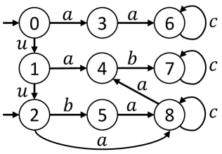
(a) System $G$ with $\Sigma_{o}=\{a,b,c\}$

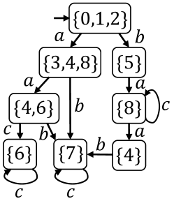
(b) $Obs(G)$

Figure 1: An arrow labeled with event $\sigma$ from state $x$ to state $x^{\prime}$ means that $x^{\prime}\in\delta(x,\sigma)$. States with arrows having no predecessor state denote initial states.

3.2 State Estimation Techniques

In this subsection, we provide techniques for computing different notions of state-estimates.

3.2.1 Computation of Current-State-Estimate

The general idea for computing the current-state-estimate is to construct a structure that tracks all possible states consistent with the current observation. This construction is well-known as the subset construction technique that can be used to convert a NFA to a DFA. In the DES literature, this structure is usually referred to as the observer automaton.

Definition 4

(Observer) Given system $G=(X,\Sigma,\delta,X_{0})$ with observable events $\Sigma_{o}\subseteq\Sigma$, the observer is a new DFA

$$Obs(G)=(X_{obs},\Sigma_{o},\delta_{obs},x_{obs,0}),$$ (11)

where $X_{obs}\subseteq 2^{X}\setminus\emptyset$ is the set of states, $x_{obs,0}=\{x\in X:\exists x_{0}\in X_{0},w\in\Sigma_{uo}^{*}\text{ s.t. }x\in\delta(x_{0},w)\}$ is the unique initial state and $\delta_{obs}$ is the deterministic transition function defined by: for any $q\in X_{obs},\sigma\in\Sigma_{o}$, we have

$$\delta_{obs}(q,\sigma)=\{x^{\prime}\in X:\exists x\in q,\exists w\in\Sigma_{uo}^{*}\text{ s.t. }x^{\prime}\in\delta(x,\sigma w)\}.$$ (12)

For the sake of simplicity, we will only consider the accessible part of $Obs(G)$.

Intuitively, the observer state tracks all possible states the system can be in currently based on the observation. Formally, we have the following result.

Proposition 1

For any system $G$ with $\Sigma_{o}\subseteq\Sigma$, its observer $Obs(G)$ has the following properties:

1. $\mathcal{L}(Obs(G))=P(\mathcal{L}(G))$; and

2. For any $\alpha\in P(\mathcal{L}(G))$, we have $\hat{X}_{G}(\alpha)=\delta_{obs}(x_{obs,0},\alpha)$.

Therefore, given an observation $\alpha\in P(\mathcal{L}(G))$, its current-state-estimate can simply be computed by Algorithm 1. Note that the complexity of building $Obs(G)$ is $O(|\Sigma|2^{|X|})$, which is exponential in the size of $G$. However, we can update the current-state-estimate recursively online and each update step only requires a polynomial complexity.

Algorithm 1 Current-State-Estimation

1:​​​​​​Inputs: $G$ and $\alpha\in P(\mathcal{L}(G))$

2:​​​​​​Output: $\hat{X}_{G}(\alpha)$

3:Build $Obs(G)=(X_{obs},\Sigma_{o},\delta_{obs},x_{obs,0})$

4:$\hat{X}_{G}(\alpha)\leftarrow\delta_{obs}(x_{obs,0},\alpha)$

5:return $\hat{X}_{G}(\alpha)$

3.2.2 Computation of Initial-State-Estimate

We provide two approaches for the computation of initial-state-estimate.

The first approach is based on the augmented automaton that augments the state-space of the original system by tracking where each state starts from. This approach sometimes is also referred to as the trellis-based approach in the literature.

Formally, given a system $G$, its augmented automaton is a new NFA

$$G_{aug}=(X_{aug},\Sigma,\delta_{aug},X_{0,aug}),$$ (13)

where $X_{aug}\subseteq X_{0}\times X$ is the set of states, $\delta_{aug}:X_{aug}\times\Sigma\to 2^{X_{aug}}$ is the transition function defined by: for any $(x_{0},x)\in X_{aug},\sigma\in\Sigma$, we have $\delta_{aug}((x_{0},x),\sigma)=\{(x_{0},x^{\prime})\in X_{0}\times X:x^{\prime}\in\delta(x,\sigma)\}$, and $X_{0,aug}=\{(x_{0},x_{0})\in X_{aug}:x_{0}\in X_{0}\}$ is the initial state.

We can see easily that $\mathcal{L}(G)=\mathcal{L}(G_{aug})$ and for each state in $G_{aug}$, its first component contains its initial state information and its second component contains its current state information. Let $Obs(G_{aug})=(X_{obs}^{aug},\Sigma_{o},\delta_{obs}^{aug},x_{obs,0}^{aug})$ be the observer of $G_{aug}$. We can easily show that

$$\hat{X}_{0,G}(\alpha)=I_{0}(\delta_{obs}^{aug}(x_{obs,0}^{aug},\alpha)),$$

where for any $q\in X_{obs}^{aug}$, $I_{0}(q)$ denotes the projection to its first component, i.e., $I_{0}(q)=\{x_{0}\in X_{0}:\exists x\in X\text{ s.t. }(x_{0},x)\in q\}$. This observation suggests Algorithm 2 for computing the initial-state-estimate.

Algorithm 2 Initial-State-Estimation-Aug

1:​​​​​​Inputs: $G$ and $\alpha\in P(\mathcal{L}(G))$

2:​​​​​​Output: $\hat{X}_{0,G}(\alpha)$

3:Build $G_{aug}$

4:Build $Obs(G_{aug})=(X_{obs}^{aug},\Sigma_{o},\delta_{obs}^{aug},x_{obs,0}^{aug})$

5:$\hat{X}_{0,G}(\alpha)\leftarrow I_{0}(\delta_{obs}^{aug}(x_{obs,0}^{aug},\alpha))$

6:return $\hat{X}_{0,G}(\alpha)$

The idea of the augmented-automaton-based approach is also very useful for many other purposes, e.g., control synthesis for initial state estimation, as it only uses the dynamic of the system up to the current point. However, the complexity of Algorithm 2 is $O(|\Sigma|2^{|X|^{2}})$ as the size of $G_{aug}$ is quadratic in the size of $G$. Here we provide the second approach for computing the initial-state-estimate with a lower complexity based on the reversed automaton of $G$.

For any NFA $G=(X,\Sigma,\delta,X_{0})$, its reversed automaton is a new NFA

$$G_{R}=(X,\Sigma,\delta_{R},X),$$ (14)

where the transition function $\delta_{R}:X\times\Sigma\to 2^{X}$ is defined by: $\forall x,x^{\prime}\in X,\sigma\in\Sigma:x^{\prime}\in\delta_{R}(x,\sigma)\Leftrightarrow x\in\delta(x^{\prime},\sigma)$. Note that the initial state of $G_{R}$ is the entire state space. For any string $s=\sigma_{1}\sigma_{2}\dots\sigma_{n}\in\Sigma^{*}$, we denote by $s_{R}$ its reversed string, i.e., $s_{R}=\sigma_{n}\dots\sigma_{2}\sigma_{1}$. Then the following result shows that the initial-state-estimate of a string in $G$ can be computed based on the current-state-estimate of its reversed string in the reversed automaton $G_{R}$.

Proposition 2

wu2013comparative For any $\alpha\in P(\mathcal{L}(G))$, we have $\hat{X}_{0,G}(\alpha)=\hat{X}_{G_{R}}(\alpha_{R})\cap X_{0}$.

Based on the above result, Algorithm 3 is proposed to compute the initial-state-estimate and its complexity is only $O(|\Sigma|2^{|X|})$.

Algorithm 3 Initial-State-Estimation-Rev

1:​​​​​​Inputs: $G$ and $\alpha\in P(\mathcal{L}(G))$

2:​​​​​​Output: $\hat{X}_{0,G}(\alpha)$

3:Build $G_{R}$

4:Build $Obs(G_{R})=(X_{obs}^{R},\Sigma_{o},\delta_{obs}^{R},X)$

5:$\hat{X}_{G_{R}}(\alpha_{R})\leftarrow\delta_{obs}^{R}(X,\alpha_{R})$

6:return $\hat{X}_{0,G}(\alpha)\leftarrow\hat{X}_{G_{R}}(\alpha_{R})\cap X_{0}$

3.2.3 Computation of Delayed-State-Estimate

For any $\alpha\beta\in P(\mathcal{L}(G))$, the delayed-state-estimate $\hat{X}_{G}(\alpha\mid\alpha\beta)$ involves two parts of information: the current information $\alpha$ and the future information $\beta$. Recall that we are interested in estimating states for the instant of $\alpha$. The following result shows that the delayed-state-estimate can simply be separated as two parts that do not depend on each other.

Proposition 3

yin2017new For any $\alpha\beta\in P(\mathcal{L}(G))$, we have

$$\hat{X}_{G}(\alpha\mid\alpha\beta)=\hat{X}_{G}(\alpha)\cap\hat{X}_{0,G}(\beta)=\hat{X}_{G}(\alpha)\cap\hat{X}_{G_{R}}(\beta_{R}).$$

Based on Proposition 3, Algorithm 4 can be used to compute the delayed-state-estimate and its complexity is also $O(|\Sigma|2^{|X|})$.

Algorithm 4 Delayed-State-Estimation

1:​​​​​​Inputs: $G$ and $\alpha\beta\in P(\mathcal{L}(G))$

2:​​​​​​Output: $\hat{X}_{G}(\alpha\mid\alpha\beta)$

3:Build $Obs(G)=(X_{obs},\Sigma_{o},\delta_{obs},x_{obs,0})$

4:$\hat{X}_{G}(\alpha)\leftarrow\delta_{obs}(x_{obs,0},\alpha)$

5:Build $G_{R}$

6:Build $Obs(G_{R})=(X_{obs}^{R},\Sigma_{o},\delta_{obs}^{R},X)$

7:$\hat{X}_{G_{R}}(\beta_{R})\leftarrow\delta_{obs}^{R}(X,\beta_{R})$

8:return $\hat{X}_{G}(\alpha\mid\alpha\beta)\leftarrow\hat{X}_{G}(\alpha)\cap\hat{X}_{G_{R}}(\beta_{R})$

Example 2

We still consider system $G$ shown in Figure 1(a), where $\Sigma_{o}=\{a,b,c\}$ and $X_{0}=\{0,2\}$. Its observer $Obs(G)$ is shown in Figure 1(b). For example, string $aa$ reaches state $\{4,6\}$ from the initial state in $Obs(G)$. Therefore, we have $\hat{X}_{G}(aa)=\{4,6\}$. To preform initial state estimation and delayed state estimation, we need to build the reversed automaton $G_{R}$ and its observer $Obs(G_{R})$ shown in Figures 2(a) and 2(b), respectively. For example, string $cba$ reaches state $\{0,1,8\}$ from the initial state in $Obs(G_{R})$. Therefore, we have $\hat{X}_{0,G}(abc)=\hat{X}_{G_{R}}((abc)_{R})\cap X_{0}=\{0,1,8\}\cap\{0,2\}=\{0\}$, i.e., we know for sure that the system was initially from state $0$. To computed the delayed-state-estimate $\hat{X}_{G}(a\mid aac)$, we have $\hat{X}_{G}(a\mid aac)=\hat{X}_{G}(a)\cap\hat{X}_{G_{R}}(ca)=\{3,4,8\}\cap\{0,1,2,3,5\}=\{3\}$.

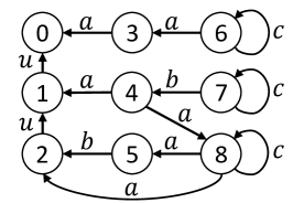
(a) $G_{R}$ with $\Sigma_{o}=\{a,b,c\}$

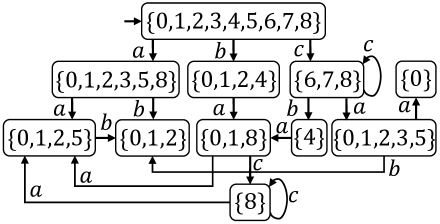
(b) $Obs(G_{R})$

Figure 2: Initial state estimation using the reversed automaton. Note that all states in $G_{R}$ are initial.

4 Properties of Partially-Observed DES

In this section, we discuss several important properties in partially-observed DES. As we mentioned before, we will only focus on observational properties.

4.1 Detectability

In the previous section, we have provided algorithms for computing state estimates. Then the natural question arises as to can the state estimation algorithm (eventually) provides precise state information. This is referred to as the detectability verification problem. Here, we consider three most fundamental types of detectability.

Definition 5

(Detectability shu2007detectability ; shu2013detectability ; shu2013delayed ) Let $G$ be a DES with $\Sigma_{o}\subseteq\Sigma$. Then $G$ is said to be

• current-state detectable if $(\exists n\in\mathbb{N})(\forall\alpha\in P(\mathcal{L}(G)):|\alpha|\geq n)[|\hat{X}_{G}(\alpha)|=1]$;

• initial-state detectable if $(\exists n\in\mathbb{N})(\forall\alpha\in P(\mathcal{L}(G)):|\alpha|\geq n)[|\hat{X}_{0,G}(\alpha)|=1]$;

• delayed detectable (w.r.t. parameters $k_{1},k_{2}\!\in\!\mathbb{N}$) if $(\forall\alpha\beta\!\in\!P(\mathcal{L}(G)):|\alpha|\geq k_{1},|\beta|\geq k_{2})[|\hat{X}_{G}(\alpha\mid\alpha\beta)|=1]$.

Intuitively, current-state detectability (respectively, initial-state detectability) requires that the current state (initial state) of the system can always be detected unambiguously within a finite delay. Note that, for initial-state-estimate, once the initial state is detected, we know it for sure forever, which is not the case for current-state-estimation. Delayed detectability requires that, for any specific instant after $k_{1}$ steps, we can always unambiguously determine the precise state of the system at that instant with at most $k_{2}$ steps of information delay. That is, one is allowed to use future information to “smooth” the state estimate of a previous instant.

The concept of detectability was initially proposed by Shu and Lin in shu2007detectability , which generalizes the concept of observability studied in ozveren1990observability . There are also other notions of detectability proposed in the literature. For example, weak detectability shu2007detectability requires that the state of the system can be detected for some path generated by the system. Also, shu2007detectability proposed the notion of periodic detectability, which requires that the state of the system can be detected periodically. In hadjicostis2016k , the authors proposed the notion of $K$-detectability by replacing the detection condition $|\hat{X}_{G}(\alpha)|=1$ as $|\hat{X}_{G}(\alpha)|\leq K$, where $K\in\mathbb{N}$ is a positive integer specifying the detection precision. A generalized version of detectability was proposed in shu2011generalized . The reader is referred to sasi2018detectability ; keroglou2017verification ; masopust2019complexity ; masopust2018complexity ; shu2008state ; yin2017verification ; zhang2017problem for more references on detectability.

4.2 Diagnosability and Prognosability of Fault

Another important application of partially-observed DES is the fault diagnosis/prognosis problem. In this setting, we assume that system $G$ may have some fault modeled as fault events $\Sigma_{F}\subseteq\Sigma$. For any string $s\in\Sigma^{*}$, we write $\Sigma_{F}\in s$ if $s$ contains a fault event in $\Sigma_{F}$. We define $\Psi(\Sigma_{F}):=\{se_{f}\in\mathcal{L}(G):e_{f}\in\Sigma_{F}\}$ as the set of strings that end up with fault events. In the fault diagnosis problem, we assume that all fault events are unobervable; otherwise, it can be diagnosed trivially. Without loss of generality, we can further assume that the state space of $G$ is partitioned as fault states and non-fault states

$$X=X_{N}\dot{\cup}X_{F},$$ (15)

such that

• $\forall x_{0}\in X_{0},\forall s\in\mathcal{L}(G,x_{0}):\Sigma_{F}\notin s\Rightarrow\delta(x_{0},s)\subseteq X_{N}$; and

• $\forall x_{0}\in X_{0},\forall s\in\mathcal{L}(G,x_{0}):\Sigma_{F}\in s\Rightarrow\delta(x_{0},s)\subseteq X_{F}$.

This assumption can be fulfilled by taking the product between $G$ and a new automaton with two states capturing the occurrence of fault; see, e.g., Lbook .

To diagnose the occurrence of fault, the current state estimation technique can be applied. Specifically, for any observation $\alpha\in P(\mathcal{L}(G))$, we know that

• the fault has occurred for sure if $\hat{X}_{G}(\alpha)\subseteq X_{F}$;

• the fault has not occurred for sure if $\hat{X}_{G}(\alpha)\subseteq X_{N}$;

• the fault may have occurred but it is uncertain if $\hat{X}_{G}(\alpha)\cap X_{N}\not=\emptyset$ and $\hat{X}_{G}(\alpha)\cap X_{F}\not=\emptyset$.

Then the natural question arises as to can we always determine the occurrence of fault within a finite number of delays. This is captured by the notion of diagnosability as follows.

Definition 6

(Diagnosability) System $G$ is said to be diagnosable w.r.t. $\Sigma_{o}$ and $\Sigma_{F}$ if $(\forall s\in\Psi(\Sigma_{F}))(\exists n\in\mathbb{N})(\forall t\in\mathcal{L}(G)/s:|t|\geq n)[\hat{X}_{G}(P(st))\subseteq X_{F}]$.

Remark 1

For the sake of simplicity, our definition of diagnosability is based on the current-state-estimate and the pre-specified fault states. Diagnosability was originally defined by sampath1995diagnosability purely based on languages as follows

$$(\forall s\!\in\!\Psi(\Sigma_{F}))(\exists n\!\in\!\mathbb{N})(\forall t\!\in\!\mathcal{L}(G)/s:|t|\geq n)(\forall w\!\in\!P^{-1}(P(st))\cap\mathcal{L}(G))[\Sigma_{F}\!\in\!w]$$

One can easily check that the language-based definition and the current-state-estimate-based definition are equivalent. Also, in general, the non-fault behavior can be described as a specification language rather than fault events; this formulation can also be transformed to our event-based fault setting by refining the state-space of the system; see, e.g., yoo2008diagnosis .

The concept of diagnosability of DES was first introduced in lin1994diagnosability , where state-based faults are considered. In sampath1995diagnosability , the authors introduced the language-based formulation of diagnosability. Since then many variations of diagnosability have been studied in the literature. For example, model reduction for diagnosability was studied in zad2003fault . Diagnosability of repeated/intermittent faults was studied in jiang2003diagnosis ; contant2004diagnosis ; fabre2018diagnosability . The reader is referred to the recent survey zaytoon2013overview for more references on diagnosability analysis.

In some applications, we may want to predict the occurrence of fault before it actually occurs. This problem is referred to as the fault prognosis problem. Still, we assume that $\Sigma_{F}\subseteq\Sigma$ is the set of fault events and $X_{N}\subseteq X$ is the set of non-fault states. However, in the fault prognosis problem, a fault event needs not be unobservable. To formulate the problem, we define the following two sets of states:

• boundary states, $\partial(G)=\{x\in X_{N}:\exists e_{f}\in\Sigma_{F}\text{ s.t. }\delta(x,e_{f})!\}$; and

• indicator states, $\Im(G)=\{x\in X_{N}:\exists n\in\mathbb{N},\forall s\in\mathcal{L}(G,x)\text{ s.t. }|s|>n\Rightarrow\Sigma_{F}\!\in\!s\}$.

Intuitively, a boundary state is a non-fault state from which a fault event may occur in the next step, and an indicator state is a state from which a fault event will occur for sure within a finite number of steps. With the help indicator states, we can also use current-state-estimation algorithm to perform online fault progsnosis. Specifically, for any observation $\alpha\in P(\mathcal{L}(G))$, we know that

• the fault will occur for sure in a finite number of steps if $\hat{X}_{G}(\alpha)\subseteq\Im(G)$;

• the fault is not guaranteed to occur within any finite number of steps if $\hat{X}_{G}(\alpha)\not\subseteq\Im(G)$.

Similarly, the natural question arises as to can we successfully predict the occurrence of fault in the sense that: (i) there is no missed fault; and (ii) there is no false alarm. This is captured by the notion of prognosability as follows.

Definition 7

(Prognosability) System $G$ is said to be prognosable w.r.t. $\Sigma_{o}$ and $\Sigma_{F}$ if $(\forall s\in\mathcal{L}(G):\delta(s)\cap\partial(G)\neq\emptyset)(\exists t\in\overline{\{s\}})[\hat{X}_{G}(P(t))\subseteq\Im(G)]$.

Prognosability is also referred to as predictability in the literature. Intuitively, prognosability requires that, for any string that reaches a boundary state, it has a prefix for which we can claim unambiguously that fault will occur for sure in the future, i.e., we can issue a fault alarm. Still, for the sake of simplicity, here we characterize prognosability using current-state-estimate, boundary states and indicator states. Our definition is also equivalent to the language-based definition in jeron2008predictability ; genc2009predictability , where predictability was originally introduced. Prognosability also has several variations in the literature. For example, in yin2016decentralized , two performance bounds were proposed to characterize how early a fault alarm can be issued and when a fault is guaranteed to occur once an alarm is issued.

4.3 State Disambiguation and Observability

In some applications, the purpose of state estimation is to distinguish some states. This problem is referred to as the state disambiguation problem wang2007algorithm ; sears2014computing ; yin2018minimization . Formally, the specification of this problem is defined as a set of state pairs $T_{spec}\subseteq X\times X$ and we want to make sure that we can always distinguish between a pair of states in $T_{spec}$.

Definition 8

(Distinguishability) System $G$ is said to be distinguishable w.r.t. $\Sigma_{o}$ and $T_{spec}\subseteq X\times X$ if $(\forall\alpha\in P(\mathcal{L}(G)))[\left(\hat{X}_{G}(\alpha)\times\hat{X}_{G}(\alpha)\right)\cap T_{spec}=\emptyset]$.

Distinguishability is very useful as many important properties in the literature can be formulated as distinguishability. For example, one can check that prognosability can actually be re-written as ditinguishability with specification $T_{spec}=\partial(G)\times(X_{N}\setminus\Im(G))$. Observability is another important property in partially-observed DES, which together with controllability provide the necessary and sufficient conditions for the existence of a supervisor achieving a desired language. The reader is referred to lin1988observability ; cieslak1988 for formal definition of observability. This property is also a special case of distinguishability (possibly after state-space refinement) as it essentially requires that we can distinguish two states at which different control actions are needed; see, e.g., wang2007algorithm .

4.4 Opacity

Finally, state estimation is also useful in information-flow security analysis, which is an important topic in cyber-physical systems. In this setting, we assume that the system is also monitored by a passive intruder (eavesdropper) that can observe the occurrences of events in $\Sigma_{o}$. Furthermore, we assume that the system has a “secret” that does not want to be revealed to the intruder. In general, what is a secret is problem dependent. Here, we consider a simple scenario where the secret is modeled as a set of secret states $X_{S}\subseteq X$. Then we use the notion of opacity to characterize whether or not the secret can be revealed to the intruder.

Definition 9

(Opacity saboori2012verification ; saboori2013verification ; wu2013comparative ; yin2017new ) Let $G$ be a DES with $\Sigma_{o}\subseteq\Sigma$ and secret states $X_{S}\subseteq X$. Then $G$ is said to be

• current-state opaque if, for any $\alpha\in P(\mathcal{L}(G))$, we have $\hat{X}_{G}(\alpha)\not\subseteq X_{S}$;

• initial-state opaque if, for any $\alpha\in P(\mathcal{L}(G))$, we have $\hat{X}_{0,G}(\alpha)\not\subseteq X_{S}$;

• infinite-step opaque if, for any $\alpha\beta\in P(\mathcal{L}(G))$, we have $\hat{X}_{G}(\alpha\mid\alpha\beta)\not\subseteq X_{S}$.

Essentially, opacity is a confidentiality property capturing the plausible deniability of the system’s “secret” in the presence of an outside observer that is potentially malicious. More specifically, current-state opacity (respectively, initial-state opacity) requires that the intruder should never know for sure that the system is currently at (respectively, initially from) a secret state. The system is said to be infinite-step opaque if the intruder can never determine for sure that the system was at a secret state for any specific instant even based on the future information.

Opacity was originally introduced in the computer science literature mazare2004using . Then it was introduced to the framework of DES by badouel2007concurrent ; bryans2008opacity ; saboori2007notions . There are also many variations of opacity studied in the literature. For example, in lin2011opacity , Lin formulated opacity using a language-based framework, where the notions of strong opacity and weak opacity are proposed. In wu2013comparative , a concept called initial-and-final-state opacity was provided; the authors also studied the transformations among several notions of opacity. When one is only allowed to used a bounded delayed information to improve the state estimate for a previous instant (or we do not care about the secret anymore after some delays), infinite-step opacity becomes to $K$-step opacity saboori2011verification , where $K$ is a non-negative integer capturing the delay bound. Opacity is also closely related to another two information-flow security properties called anonymity sweeney2002k and non-interference hadj2005verification ; hadj2005characterizing . The reader is referred to the survey jacob2016overview for more references on opacity.

5 Verification Techniques

In this section, we provide techniques for verifying observational properties introduced in the previous section. First, we show that most of the properties in partially-observed DES can be verified using the observer structure and some important properties can be more efficienty verified using the twin-plant technique in polynomial-time.

5.1 Observer-Based Verification

5.1.1 Verification of Detectability

First, we study the verification of current-state detectability. Recall that, current-state detectability requires that $(\exists n\in\mathbb{N})(\forall\alpha\in P(\mathcal{L}(G)):|\alpha|\geq n)[|\hat{X}_{G}(\alpha)|=1]$. In other words, a system is not current-state detectable if there is an arbitrarily long observation string such that the current-state-estimate is not always a singleton starting from any instant. Since $P(\mathcal{L}(G))$ is a regular language, due to the Pumping lemma, the existence of such an arbitrarily long string is equivalent to the existence of a cycle in $Obs(G)$ in which a state is not a singleton. This immediately suggests Algorithm 5 for the verification of current-state detectability. Initial-state detectability can also be checked in the same manner using $G_{aug}$. The only differences from Algorithm 5 are (i) we need to consider $Obs(G_{aug})$ rather than $Obs(G)$ in line 1; and (ii) in line 2, we need to check the existence of a cycle $q_{0}q_{1}\dots q_{n}$ in $Obs(G_{aug})$ such that $|I_{0}(q_{i})|>1$ for some $i=1,\dots,n$.

Algorithm 5 Cur-State-Dect-Ver-Obs

1:​​​​​​Inputs: $G$

2:​​​​​​Output: Current-State Detectable or Not

3:Build $Obs(G)=(X_{obs},\Sigma_{o},\delta_{obs},x_{obs,0})$

4:if there exists a cycle $q_{0}q_{1}\dots q_{n}$ in $Obs(G)$ such that $|q_{i}|>1$ for some $i=1,\dots,n$ then

5:     return $G$ is not current-state detectable

6:else

7:     return $G$ is current-state detectable

8:end if

To check delayed detectability (for parameters $k_{1},k_{2}\in\mathbb{N}$), first we recall that the delayed-state-estimate can be computed by $\hat{X}_{G}(\alpha\mid\alpha\beta)=\hat{X}_{G}(\alpha)\cap\hat{X}_{G_{R}}(\beta_{R})$. Therefore, delayed detectability can be checked by the following steps:

• First, we compute all possible current-state-estimate $\hat{X}_{G}(\alpha)$ reachable via some string $\alpha$ whose length is greater than or equal to $k_{1}$;

• Then, we compute all possible current-state-estimate of $\hat{X}_{G_{R}}(\beta_{R})$ in $G_{R}$ reachable via some string $\beta_{R}$ whose length is greater than or equal to $k_{2}$;

• Finally, we test whether or not there exist such $\hat{X}_{G}(\alpha)$ and $\hat{X}_{G_{R}}(\beta_{R})$ such that $|\hat{X}_{G}(\alpha)\cap\hat{X}_{G_{R}}(\beta_{R})|>1$. If so, then it means that some instant after $k_{1}$ steps cannot be determined within $k_{2}$ steps of delay, i.e, the system is not delayed detectable.

This procedure is formalized by Algorithm 6, where states in lines 3 and 4 can be computed by a simple depth-first search or a breath-first search.

Algorithm 6 Delay-State-Dect-Ver-Obs

1:​​​​​​Inputs: $G$

2:​​​​​​Output: Delayed Detectable or Not

3:Build $Obs(G)=(X_{obs},\Sigma_{o},\delta_{obs},x_{obs,0})$

4:Build $Obs(G_{R})=(X_{obs}^{R},\Sigma_{o},\delta_{obs}^{R},X)$

5:for all $q_{1}\in X_{obs}$ that be can reached by a string longer than $k_{1}$ in $Obs(G)$ do

6:     for all $q_{2}\in X_{obs}^{R}$ that be can reached by a string longer than $k_{2}$ in $Obs(G_{R})$ do

7:         if $|q_{1}\cap q_{2}|>1$ then

8:              return $G$ is not delayed detectable

9:         end if

10:     end for

11:end for

12:return $G$ is delayed detectable

5.1.2 Verification of Diagnosability

The verification of diagnosability is very similar to the case of current-state detectability. Specifically, a system is not diagnosable if there is an arbitrarily long string after the occurrence of fault such that the current-state-estimate is not a subset of $X_{N}$ starting from any instant. Therefore, the general idea is to replaced condition $|q_{i}|>1$ in Algorithm 5 by $q_{i}\not\subseteq X_{F}$. However, we need to do a little bit more here since we are only interested in arbitrarily long uncertain strings after the occurrence of fault; this is also referred to as an indeterminate cycles in the literature sampath1995diagnosability . In other words, the existence of an arbitrarily long uncertain but non-fault string does not necessarily violate diagnosability.

To this end, we need to compose $Obs(G)$ with the dynamic of the original system $G$. Specifically, let $Obs(G)$ be the observer of $G$. We define

$$\widetilde{Obs}(G)=(X_{obs},\Sigma,\tilde{\delta}_{obs},x_{obs,0})$$ (16)

as the DFA by adding self-loops of all unobservable events at each state in $X_{obs}$. One can easily check that $\mathcal{L}(G)=\mathcal{L}(G\times\widetilde{Obs}(G))$. Then, by looking at the first component of each state in $G\times\widetilde{Obs}(G)$, we know whether a fault event has occurred or not. Therefore, we can check diagnosability based on $G\times\widetilde{Obs}(G)$ by Algorithm 7.

Algorithm 7 Diag-Ver-Obs

1:​​​​​​Inputs: $G$ and $\Sigma_{F}$

2:​​​​​​Output: Diagnosable or Not

3:Build $Obs(G)=(X_{obs},\Sigma_{o},\delta_{obs},x_{obs,0})$

4:Augment $Obs(G)$ as $\widetilde{Obs}(G)=(X_{obs},\Sigma,\tilde{\delta}_{obs},x_{obs,0})$ by adding unobservable self-loops

5:Compute $G\times\widetilde{Obs}(G)$

6:if there exists a cycle $(x_{0},q_{0})(x_{1},q_{1})\dots(x_{n},q_{n})$ in $G\times\widetilde{Obs}(G)$ such that $x_{i}\in X_{F}$ and $q_{i}\not\subseteq X_{F}$ for some $i=1,\dots,n$ then

7:     return $G$ is not diagnosable

8:else

9:     return $G$ is diagnosable

10:end if

5.1.3 Verification of Distinguishability and Opacity

The verification of distinguishability is straightforward using the observer. Specifically, we just need to check whether or not there exists a state $q\in X_{obs}$ in $Obs(G)$ such that $(q\times q)\cap T_{spec}\not=\emptyset$. If so, the system is not distinguishable; otherwise, it is distinguishable. Since we have discussed that prognosability is a special case of distinguishability, it can also be checked in the same manner.

Similarly, current-state opacity can be verified by checking whether or not there exists a state $q\in X_{obs}$ in $Obs(G)$ such that $q\subseteq X_{S}$. If so, the system is not opaque; otherwise, it is opaque. To check initial-state opacity, we need to construct $Obs(G_{R})$ and to check whether or not there exists a state $q\in X_{obs}^{R}$ in $Obs(G_{R})$ such that $q\cap X_{0}\subseteq X_{S}$.

The verification of infinite-step opacity is similar to the case of delayed detectability; both involve delayed-state-estimate that can be computed according to Proposition 3. The verification procedure for infinite-step opacity is provided in Algorithm 8 with complexity $O(|\Sigma|4^{|X|})$.

Algorithm 8 Inf-Opa-Ver-Obs

1:​​​​​​Inputs: $G$

2:​​​​​​Output: Infinite-Step Opaque or Not

3:Build $Obs(G)=(X_{obs},\Sigma_{o},\delta_{obs},x_{obs,0})$

4:Build $Obs(G_{R})=(X_{obs}^{R},\Sigma_{o},\delta_{obs}^{R},X)$

5:for all $q_{1}\in X_{obs}$ do

6:     for all $q_{2}\in X_{obs}^{R}$ do

7:         if $\emptyset\neq q_{1}\cap q_{2}\subseteq X_{S}$ then

8:              return $G$ is not infinite-step opaque

9:         end if

10:     end for

11:end for

12:return $G$ is infinite-step opaque

5.2 Twin-Plant-Based Verification

In the previous section, we have shown that the observer can be used for the verification of all properties introduced. However, the size of the observer is exponential in the size of the system. Then the natural question arises as to can we find polynomial-time algorithms for verifying these properties. Unfortunately, it has been shown in cassez2012synthesis that deciding opacity is PSPACE-complete; hence, no polynomial-time algorithm exists. However, it is indeed possible to check diagnosability, detectability and distinguishability in polynomial-time by using the twin-plant structure. This structure was originally proposed in tsitsiklis1989control for the verification of observability; later on it has been used for verifying diagnosability (under the name of “verifier”) by jiang2001polynomial ; yoo2002polynomial and for verifying detectability (under the name of “detector”) by shu2010detectability .

Definition 10

(Twin-Plant) Given system $G=(X,\Sigma,\delta,X_{0})$ with observable events $\Sigma_{o}\subseteq\Sigma$, the twin-plant is a new NFA $V(G)=(X_{V},\Sigma_{V},\delta_{V},X_{0,V})$, where

• $X_{V}\subseteq X\times X$ is the set of states;

• $\Sigma_{V}=(\Sigma_{o}\times\Sigma_{o})\cup(\Sigma_{uo}\times\{\epsilon\})\cup(\{\epsilon\}\times\Sigma_{uo})$ is the set of events;

• $X_{0,V}=X_{0}\times X_{0}$ is the set of initial states;

• $\delta_{V}:X_{V}\times\Sigma_{V}\rightarrow 2^{X_{V}}$ is the partial transition function defined by: for any state $(x_{1},x_{2})\in X_{V}$ and event $\sigma\in\Sigma$

(a) If $\sigma\in\Sigma_{o}$, then the following transition is defined

$$\delta_{V}((x_{1},x_{2}),(\sigma,\sigma))=\delta(x_{1},\sigma)\times\delta(x_{2},\sigma)$$ (17)

(a) If $\sigma\in\Sigma_{uo}$, then the following transitions are defined

$$\delta_{V}((x_{1},x_{2}),(\sigma,\epsilon)) =\delta(x_{1},\sigma)\times\{x_{2}\}$$ (18)

$$\delta_{V}((x_{1},x_{2}),(\epsilon,\sigma)) =\{x_{1}\}\times\delta(x_{2},\sigma)$$ (19)

Hereafter, we only consider the accessible part of $V(G)$.

Intuitively, the twin-plant $V$ tracks all pairs of observation equivalent strings in $G$. Specifically, if $s_{1},s_{2}\in\mathcal{L}(G)$ are two strings in $G$ such that $P(s_{1})=P(s_{2})$, then there exists a string $s\in\mathcal{L}(V(G))$ in $V(G)$ such that its first and second components are $s_{1}$ and $s_{2}$, respectively. On the other hand, for any string $s=(s_{1},s_{2})\in\mathcal{L}(V(G))$ in $V(G)$, we have that $P(s_{1})=P(s_{2})$.

The twin-plant can be applied directly for the verification of distinguishability. Specifically, we need to check if $V(G)$ contains a pair of states in the specification. This procedure is presented in Algorithm 9.

According to the definition of detectability, we know that the system is not detectable if and only if there exist two arbitrarily long strings having the same observation, such that these two strings lead to two different states. As we discussed above, all such string pairs can be captured by the twin-plant. This suggests Algorithm 10 for the verification of current-state detectability.

The case of diagnosability is similar. Specifically, a system is not diagnosable if there exist an arbitrarily long fault string and a non-fault string such that they have the same observation. This condition can be checked by Algorithm 11. Note that, we have already assumed that there is no unobservable cycle in $G$. Otherwise, we need to add the following condition to the “if condition” in line 2 of Algorithm 11 to obtain an arbitrarily long fault string:

$$\exists j=0,\dots,n-1,\exists\sigma_{V}\notin\Sigma_{uo}\times\{\epsilon\}:(x_{j+1}^{1},x_{j+1}^{2})\in\delta_{V}((x_{j}^{1},x_{j}^{2}),\sigma_{V}).$$

Since the size of the twin-plant is only quadratic in the size of $G$, distinguishability, detectability and diagnosability can all be checked in polynomial-time, which is better than the observer-based approach.

Algorithm 9 Dist-Ver-Obs

1:​​​​​​Inputs: $G$ and $T_{spec}$

2:​​​​​​Output: Distinguishable or Not

3:Build $V(G)=(X_{V},\Sigma_{V},\delta_{V},X_{0,V})$

4:if there exists a state $(x_{1},x_{2})\in X_{V}$ in $V(G)$ such that $(x_{1},x_{2})\in T_{spec}$ then

5:     return $G$ is not distinguishable

6:else

7:     return $G$ is distinguishable

8:end if

Algorithm 10 Cur-State-Dect-Ver-Obs

1:​​​​​​Inputs: $G$ and $\Sigma_{F}$

2:​​​​​​Output: Current-State Detectable or Not

3:Build $V(G)=(X_{V},\Sigma_{V},\delta_{V},X_{0,V})$

4:if there exists a cycle $(x_{0}^{1},x_{0}^{2})(x_{1}^{1},x_{1}^{2})\dots(x_{n}^{1},q_{n}^{2})$ in $V(G)$ such that $\exists i\!=\!0,\dots,n:x_{i}^{1}\!\not=\!x_{i}^{2}$ then

5:     return $G$ is not current-state detectable

6:else

7:     return $G$ is current-state detectable

8:end if

Algorithm 11 Diag-Ver-TP

1:​​​​​​Inputs: $G$ and $\Sigma_{F}$

2:​​​​​​Output: Diagnosable or Not

3:Build $V(G)=(X_{V},\Sigma_{V},\delta_{V},X_{0,V})$

4:if there exists a cycle $(x_{0}^{1},x_{0}^{2})(x_{1}^{1},x_{1}^{2})\dots(x_{n}^{1},q_{n}^{2})$ in $V(G)$ such that

5:$\forall i=0,\dots,n:x_{i}^{1}\in X_{N}\wedge x_{i}^{2}\in X_{F}$ then

6:     return $G$ is not diagnosable

7:else

8:     return $G$ is diagnosable

9:end if

6 Related Problems and Further Readings

6.1 State Estimation under General Observation Models

Throughout this article, we assume that the observation of the system is modeled as a natural projection. The natural projection mapping is essentially static in the sense that an event is always either observable or unobservable. One related topic is the sensor selection problem for static observations haji1996minimizing ; yoo2002np ; jiang2003optimal ; ru2010sensor ; cabasino2013optimal , i.e., we want to decide which events should be observable by placing with sensors such that a given observational property is fulfilled. Another related topic in the static observation setting is the robust state estimation problem when the observation is unreliable. This problem has been investigated in the context of detectability analysis yin2017initial , diagnosability anlaysis thorsley2008diagnosability ; takai2012verification ; carvalho2012robust ; carvalho2013robust and supervisory control rohloff2005sensor ; sanchez2006safe ; lin2014control ; alves2014robust ; ushio2016nonblocking ; yin2017supervisor for partially-observed DES.

In many situations, due to information communications and acquisitions, the observation mapping may be dynamic, i.e., whether or not an event is observable depends the trajectory of the system. One example is the dynamic sensor activation problem, where we can decide to turn sensors on/off dynamically online based on the observation history. In thorsley2007active ; cassez2008fault ; wang2010optimal ; dallal2014most , the fault diagnosis problem is studied under the dynamic observation setting. In huang2008decentralized ; wang2010minimization , observability is studied under the dynamic observation setting. In shu2010detectability ; shu2013online , the authors investigated the verification and synthesis of detectability under dynamic observations. Opacity under dynamic observations is also studied in cassez2012synthesis ; zhang2015max . A general approach for dynamic sensor activation for property enforcement is proposed by yin2019general . In wang2011codiagnosability ; yin2015codiagnosability , it has been shown that (co)diagnosability and (co)observability can be mapped from one to the other in the general dynamic observation setting. The reader is referred to the recent survey sears2016minimal for more references on state estimation problem under dynamic observations.

6.2 State Estimation in Coordinated, Distributed and Modular Systems

In the setting of this article, we only consider the scenario where the system is monitored by a single observer, which is referred to as the centralized state estimation. In many large-scale systems, sensors can be physically distributed and the system can be monitored by multiple local observers that have incomparable information. Each local observer can perform local state estimation and send it to a coordinator. Then the coordinator will fuses all local information according to some pre-specified protocol in order to obtain a global estimation decision. This is referred to as the decentralized estimation and decision making problem under coordinated architecture.

In the context of DES, the decentralized estimation and decision making problem was first studied by cieslak1988 ; rudie1992think ; rudie1995computational in the context of decentralized supervisory control, where the notion of coobservability is proposed. In debouk2000coordinated ; wang2007diagnosis , the problem of decentralized fault diagnosis problem was studied and a corresponding property called codiagnosability was proposed; the verification codiagnosability has also been studied in the literature moreira2011polynomial ; qiu2006decentralized . The decentralized fault prognosis has also been studied in the literature; see, e.g., kumar2010decentralized ; khoumsi2012conjunctive ; yin2016decentralized2 . Note that, in decentralized decision making problems, one important issue is the underlying coordinated architecture. For example, rudie1992think and qiu2006decentralized only consider simple binary architectures for control and diagnosis, respectively; more complicated architectures can be found in yoo2002general ; yoo2004decentralized ; kumar2009inference ; kumar2007inference ; takai2011inference ; chakib2011multi ; ricker2007knowledge ; yin2016decentralized ; khoumsi2018decentralized .

When each local observer is allow to communicate and exchange information with each other, the state estimation problem is referred to as the distributed estimation problem. Works on distributed state estimation and property verification can be founded in benveniste2003diagnosis ; su2005global ; genc2007distributed ; takai2012distributed . Finally, state estimation and verification of partially-observed modular DES have also been considered in the literature rohloff2005pspace ; contant2006diagnosability ; saboori2010reduced ; schmidt2013verification ; yin2017verification ; masopust2019complexity , where a modular system is composed by a set of local modules in the form of $G=G_{1}\times\cdots\times G_{n}$.

6.3 Estimation and Verification of Petri Nets and Stochastic DES

In this article, we focus on DES modeled as finite state automata. Petri nets, another important class of DES models, are widely used to model many classes of concurrent systems. In particular, Petri nets provide a compact model without enumerating the entire state space and it is well-known that Petri net languages are more expressive than regular languages. The problems of state estimation and property verification have also drawn many attentions in the context of Petri nets. For example, state (marking) estimation algorithms for Petri nets have been proposed in giua2007marking ; li2013minimum ; bonhomme2015marking ; basile2015state . Decidability and verification procedures for diagnosability berard2018complexity ; ran2018codiagnosability ; basile2012k ; cabasino2012new ; yin2017decidability , detectability masopust2018deciding ; giua2002observability , prognosability yin2018verification and opacity tong2017verification ; tong2017decidability are also studied in the literature for Petri nets.

Another important generalization of the finite state automata model is the stochastic DES (or labelled Markov chains). Stochastic DES can not only characterize whether or not a system can reach a state, it can also capture the possibility of reaching a state. Hence it provides a model for the quantitative analysis and verification of DES. State estimation and verification of many important properties have also been extended to the stochastic DES setting; this includes, e.g., diagnosability yin2019robust ; liu2008decentralized ; thorsley2005diagnosability , detectability shu2008state ; keroglou2017verification ; yin2017initial ; zhao2019detectability , prognosability chen2015stochastic and opacity saboori2014current ; berard2015probabilistic ; yin2019infinite .

6.4 Control Synthesis of Partially-Observed DES

So far, we have only discussed property verification problems in partially-observed DES. In many applications, when the answer to the verification problem is negative, it is important to synthesize a supervisor or controller that provably enforces the property by restricting the system behavior but as permissive as possible. This control synthesis problem has been studied in the literature in the framework of the supervisory control theory initiated by Ramadge and Wonham ramadge1987supervisory . The reader is referred to the textbooks Lbook ; Cbook for more details on supervisory control of DES. Supervisory control under partial observation was originally investigated by cieslak1988 ; lin1988observability . Since then, many control synthesis algorithms for partial-observation supervisors have been proposed cho1989supremal ; kumar1991controllability ; takai2003effective ; yoo2006solvability ; cai2015relative . In particular, yin2016synthesis solves the synthesis problem for maximally-permissive non-blocking supervisors in the partial observation setting.

In the context of enforcement of observational properties, in sampath1998active , an approach was proposed for designing a supervisor that enforces diagnosability. Control synthesis algorithms have also been proposed in the literature for enforcing opacity; see, e.g. dubreil2010supervisory ; tong2018current ; saboori2012opacity . In shu2013enforcing , the authors studied the problem of synthesizing supervisors that enforce detectability. A uniform approach for control synthesis for enforcing a wide class of properties was recently proposed by Yin and Lafortune in a series of papers yin2018synthesis ; yin2017synthesis ; yin2016synthesis ; yin2016uniform .

References

- [1] M.V.S. Alves, J.C. Basilio, A.E. Carrilho da Cunha, L.K. Carvalho, and M.V. Moreira. Robust supervisory control against intermittent loss of observations. In 12th International Workshop on Discrete Event Systems, volume 12, pages 294–299, 2014.
- [2] E. Badouel, M. Bednarczyk, A. Borzyszkowski, B. Caillaud, and P. Darondeau. Concurrent secrets. Discrete Event Dynamic Systems: Theory & Applications, 17(4):425–446, 2007.
- [3] F. Basile, M.P. Cabasino, and C. Seatzu. State estimation and fault diagnosis of labeled time petri net systems with unobservable transitions. IEEE Transactions on Automatic Control, 60(4):997–1009, 2015.
- [4] F. Basile, P. Chiacchio, and G. De Tommasi. On -diagnosability of Petri nets via integer linear programming. Automatica, 48(9):2047–2058, 2012.
- [5] N. Ben Hadj-Alouane, S. Lafrance, F. Lin, J. Mullins, and M. Yeddes. Characterizing intransitive noninterference for 3-domain security policies with observability. IEEE Transactions on Automatic Control, 50(6):920–925, 2005.
- [6] N. Ben Hadj-Alouane, S. Lafrance, F. Lin, J. Mullins, and M. Yeddes. On the verification of intransitive noninterference in mulitlevel security. IEEE Transactions on Systems, Man, and Cybernetics, Part B (Cybernetics), 35(5):948–958, 2005.
- [7] A. Benveniste, E. Fabre, S. Haar, and C. Jard. Diagnosis of asynchronous discrete-event systems: a net unfolding approach. IEEE Transactions on Automatic Control, 48(5):714–727, 2003.
- [8] B. Bérard, K. Chatterjee, and N. Sznajder. Probabilistic opacity for markov decision processes. Information Processing Letters, 115(1):52–59, 2015.
- [9] B. Bérard, S. Haar, S. Schmitz, and S. Schwoon. The complexity of diagnosability and opacity verification for Petri nets. Fundamenta Informaticae, 161(4):317–349, 2018.
- [10] P. Bonhomme. Marking estimation of p-time Petri nets with unobservable transitions. IEEE Transactions on Systems, Man, and Cybernetics: Systems, 45(3):508–518, 2015.
- [11] J.W. Bryans, M. Koutny, L. Mazaré, and P.Y.A. Ryan. Opacity generalised to transition systems. International Journal of Information Security, 7(6):421–435, 2008.
- [12] M.P. Cabasino, A. Giua, S. Lafortune, and C. Seatzu. A new approach for diagnosability analysis of Petri nets using verifier nets. IEEE Transactions on Automatic Control, 57(12):3104–3117, 2012.
- [13] M.P. Cabasino, S. Lafortune, and C. Seatzu. Optimal sensor selection for ensuring diagnosability in labeled Petri nets. Automatica, 49(8):2373–2383, 2013.
- [14] K. Cai, R. Zhang, and W.M. Wonham. Relative observability of discrete-event systems and its supremal sublanguages. IEEE Transactions on Automatic Control, 60(3):659–670, 2015.
- [15] L. K. Carvalho, M.V. Moreira, J.C. Basilio, and S. Lafortune. Robust diagnosis of discrete-event systems against permanent loss of observations. Automatica, 49(1):223–231, 2013.
- [16] L.K. Carvalho, J.C. Basilio, and M.V. Moreira. Robust diagnosis of discrete event systems against intermittent loss of observations. Automatica, 48(9):2068–2078, 2012.
- [17] C.G. Cassandras and S. Lafortune. Introduction to Discrete Event Systems. Springer, 2nd edition, 2008.
- [18] F. Cassez, J. Dubreil, and H. Marchand. Synthesis of opaque systems with static and dynamic masks. Formal Methods in System Design, 40(1):88–115, 2012.
- [19] F. Cassez and S. Tripakis. Fault diagnosis with static and dynamic observers. Fundamental Informaticae, 88(4):497–540, 2008.
- [20] H. Chakib and A. Khoumsi. Multi-decision supervisory control: Parallel decentralized architectures cooperating for controlling discrete event systems. IEEE Transactions on Automatic Control, 56(11):2608–2622, 2011.
- [21] J. Chen and R. Kumar. Stochastic failure prognosability of discrete event systems. IEEE Transactions on Automatic Control, 60(6):1570–1581, 2015.
- [22] H. Cho and S.I. Marcus. Supremal and maximal sublanguages arising in supervisor synthesis problems with partial observations. Mathematical Systems Theory, 22(1):177–211, 1989.
- [23] R. Cieslak, C. Desclaux, A.S. Fawaz, and P. Varaiya. Supervisory control of discrete-event processes with partial observations. IEEE Transactions on Automatic Control, 33(3):249–260, 1988.
- [24] O. Contant, S. Lafortune, and D. Teneketzis. Diagnosis of intermittent faults. Discrete Event Dynamic Systems: Theory & Applications, 14(2):171–202, 2004.
- [25] O. Contant, S. Lafortune, and D. Teneketzis. Diagnosability of discrete event systems with modular structure. Discrete Event Dynamic Systems: Theory & Applications, 16(1):9–37, 2006.
- [26] E. Dallal and S. Lafortune. On most permissive observers in dynamic sensor activation problems. IEEE Transactions on Automatic Control, 59(4):966–981, 2014.
- [27] R. Debouk, S. Lafortune, and D. Teneketzis. Coordinated decentralized protocols for failure diagnosis of discrete event systems. Discrete Event Dynamic Systems: Theory & Applications, 10(1-2):33–86, 2000.
- [28] J. Dubreil, P. Darondeau, and H. Marchand. Supervisory control for opacity. IEEE Transactions on Automatic Control, 55(5):1089–1100, 2010.
- [29] E. Fabre, L. Hélouët, E. Lefaucheux, and H. Marchand. Diagnosability of repairable faults. Discrete Event Dynamic Systems: Theory & Applications, 28(2):183–213, 2018.
- [30] S. Genc and S. Lafortune. Distributed diagnosis of place-bordered Petri nets. IEEE Transactions on Automation Science and Engineering, 4(2):206–219, 2007.
- [31] S. Genc and S. Lafortune. Predictability of event occurrences in partially-observed discrete-event systems. Automatica, 45(2):301–311, 2009.
- [32] A. Giua and C. Seatzu. Observability of place/transition nets. IEEE Transactions on Automatic Control, 47(9):1424–1437, 2002.
- [33] A. Giua, C. Seatzu, and D. Corona. Marking estimation of Petri nets with silent transitions. IEEE Transactions on Automatic Control, 52(9):1695–1699, 2007.
- [34] C.N. Hadjicostis and C. Seatzu. K-detectability in discrete event systems. In 55th IEEE Conference on Decision and Control, pages 420–425, 2016.
- [35] A. Haji-Valizadeh and K. Loparo. Minimizing the cardinality of an events set for supervisors of discrete-event dynamical systems. IEEE Transactions on Automatic Control, 41(11):1579–1593, 1996.
- [36] Y. Huang, K. Rudie, and F. Lin. Decentralized control of discrete-event systems when supervisors observe particular event occurrences. IEEE Transactions on Automatic Control, 53(1):384–388, 2008.
- [37] R. Jacob, J.-J. Lesage, and J.-M. Faure. Overview of discrete event systems opacity: Models, validation, and quantification. Annual Reviews in Control, 41:135–146, 2016.
- [38] T. Jéron, H. Marchand, S. Genc, and S. Lafortune. Predictability of sequence patterns in discrete event systems. IFAC Proceedings Volumes, 41(2):537–543, 2008.
- [39] S. Jiang, Z. Huang, V. Chandra, and R. Kumar. A polynomial algorithm for testing diagnosability of discrete-event systems. IEEE Transactions on Automatic Control, 46(8):1318–1321, 2001.
- [40] S. Jiang, R. Kumar, and H.E Garcia. Optimal sensor selection for discrete-event systems with partial observation.
- [41] S. Jiang, R. Kumar, and H.E. Garcia. Diagnosis of repeated/intermittent failures in discrete event systems. IEEE Transactions on Robotics and Automation, 19(2):310–323, 2003.
- [42] C. Keroglou and C.N. Hadjicostis. Verification of detectability in probabilistic finite automata. Automatica, 86:192–198, 2017.
- [43] A. Khoumsi and H. Chakib. Conjunctive and disjunctive architectures for decentralized prognosis of failures in discrete-event systems. IEEE Transactions on Automation Science and Engineering, 9(2):412–417, 2012.
- [44] A. Khoumsi and H. Chakib. Decentralized supervisory control of discrete event systems: An arborescent architecture to realize inference-based control. IEEE Transactions on Automatic Control, 63(12):4278–4285, 2018.
- [45] R. Kumar, V. Garg, and S.I. Marcus. On controllability and normality of discrete event dynamical systems. Systems & Control Letters, 17(3):157–168, 1991.
- [46] R. Kumar and S. Takai. Inference-based ambiguity management in decentralized decision-making: Decentralized control of discrete event systems. IEEE Transactions on Automatic Control, 52(10):1783–1794, 2007.
- [47] R. Kumar and S. Takai. Inference-based ambiguity management in decentralized decision-making: Decentralized diagnosis of discrete-event systems. IEEE Transactions on Automation Science and Engineering, 6(3):479–491, 2009.
- [48] R. Kumar and S. Takai. Decentralized prognosis of failures in discrete event systems. IEEE Transactions on Automatic Control, 55(1):48–59, 2010.
- [49] L. Li and C.N. Hadjicostis. Minimum initial marking estimation in labeled Petri nets. IEEE Transactions on Automatic Control, 58(1):198–203, 2013.
- [50] F. Lin. Diagnosability of discrete event systems and its applications. Discrete Event Dynamic Systems: Theory & Applications, 4(2):197–212, 1994.
- [51] F. Lin. Opacity of discrete event systems and its applications. Automatica, 47(3):496–503, 2011.
- [52] F. Lin. Control of networked discrete event systems: dealing with communication delays and losses. SIAM Journal onn Control and Optimization, 52(2):1276–1298, 2014.
- [53] F. Lin and W.M. Wonham. On observability of discrete-event systems. Information Sciences, 44(3):173–198, 1988.
- [54] F. Liu, D. Qiu, H. Xing, and Z. Fan. Decentralized diagnosis of stochastic discrete event systems. IEEE Transactions on Automatic Control, 53(2):535–546, 2008.
- [55] T. Masopust. Complexity of deciding detectability in discrete event systems. Automatica, 93:257–261, 2018.
- [56] T. Masopust and X. Yin. Complexity of detectability, opacity and a-diagnosability for modular discrete event systems. Automatica, 101:290–295, 2019.
- [57] T. Masopust and X. Yin. Deciding detectability for labeled Petri nets. Automatica, 2019.
- [58] L. Mazaré. Using unification for opacity properties. In Proceedings of WITS, volume 4, pages 165–176, 2004.
- [59] M. V. Moreira, T. C. Jesus, and J. C. Basilio. Polynomial time verification of decentralized diagnosability of discrete event systems. IEEE Transactions on Automatic Control, 56(7):1679–1684, 2011.
- [60] C.M. Ozveren and A.S. Willsky. Observability of discrete event dynamic systems. IEEE Transactions on Automatic Control, 35(7):797–806, 1990.
- [61] W. Qiu and R. Kumar. Decentralized failure diagnosis of discrete event systems. IEEE Transactions on Systems, Man and Cybernetics, Part A, 36(2):384–395, 2006.
- [62] P.J. Ramadge and W.M. Wonham. Supervisory control of a class of discrete event processes. SIAM Journal on Control and Optimization, 25(1):206–230, 1987.
- [63] N. Ran, H. Su, A. Giua, and C. Seatzu. Codiagnosability analysis of bounded Petri nets. IEEE Transactions on Automatic Control, 63(4):1192–1199, 2018.
- [64] S.L. Ricker and K. Rudie. Knowledge is a terrible thing to waste: Using inference in discrete-event control problems. IEEE Transactions on Automatic Control, 52(3):428–441, 2007.
- [65] K. Rohloff. Sensor failure tolerant supervisory control. In 44th IEEE Conf. Decision and Control, pages 3493–3498, 2005.
- [66] K. Rohloff and S. Lafortune. PSPACE-completeness of modular supervisory control problems. Discrete Event Dynamic Systems: Theory & Applications, 15(2):145–167, 2005.
- [67] Y. Ru and C.N. Hadjicostis. Sensor selection for structural observability in discrete event systems modeled by Petri nets. IEEE Transactions on Automatic Control, 55(8):1751–1764, 2010.
- [68] K. Rudie and J. C. Willems. The computational complexity of decentralized discrete-event control problems. IEEE Transactions on Automatic Control, 40(7):1313–1319, 1995.
- [69] K. Rudie and W. M. Wonham. Think globally, act locally: Decentralized supervisory control. IEEE Transactions on Automatic Control, 37(11):1692–1708, 1992.
- [70] A. Saboori and C. N. Hadjicostis. Opacity-enforcing supervisory strategies via state estimator constructions. IEEE Transactions on Automatic Control, 57(5):1155–1165, 2012.
- [71] A. Saboori and C.N. Hadjicostis. Notions of security and opacity in discrete event systems. In 46th IEEE Conference on Decision and Control, pages 5056–5061. IEEE, 2007.
- [72] A. Saboori and C.N. Hadjicostis. Reduced-complexity verification for initial-state opacity in modular discrete event systems. IFAC Proceedings Volumes, 43(12):78–83, 2010.
- [73] A. Saboori and C.N. Hadjicostis. Verification of -step opacity and analysis of its complexity. IEEE Transactions on Automation Science and Engineering, 8(3):549–559, 2011.
- [74] A. Saboori and C.N. Hadjicostis. Verification of infinite-step opacity and complexity considerations. IEEE Transactions on Automatic Control, 57(5):1265–1269, 2012.
- [75] A. Saboori and C.N. Hadjicostis. Verification of initial-state opacity in security applications of discrete event systems. Information Sciences, 246:115–132, 2013.
- [76] A. Saboori and C.N. Hadjicostis. Current-state opacity formulations in probabilistic finite automata. IEEE Transactions on Automatic Control, 59(1):120–133, 2014.
- [77] M. Sampath, S. Lafortune, and D. Teneketzis. Active diagnosis of discrete-event systems. IEEE Transactions on Automatic Control, 43(7):908–929, 1998.
- [78] M. Sampath, R. Sengupta, S. Lafortune, K. Sinnamohideen, and D. Teneketzis. Diagnosability of discrete-event systems. IEEE Transactions on Automatic Control, 40(9):1555–1575, 1995.
- [79] A.M. Sánchez and F.J. Montoya. Safe supervisory control under observability failure. Discrete Event Dynamic Systems: Theory & Applications, 16(4):493–525, 2006.
- [80] Y. Sasi and F. Lin. Detectability of networked discrete event systems. Discrete Event Dynamic Systems: Theory & Applications, 28(3):449–470, 2018.
- [81] K.W. Schmidt. Verification of modular diagnosability with local specifications for discrete-event systems. IEEE Transactions on Systems, Man, and Cybernetics: Systems, 43(5):1130–1140, 2013.
- [82] D. Sears and K. Rudie. On computing indistinguishable states of nondeterministic finite automata with partially observable transitions. In 53rd IEEE Conference on Decision and Control, pages 6731–6736, 2014.
- [83] D. Sears and K. Rudie. Minimal sensor activation and minimal communication in discrete-event systems. Discrete Event Dynamic Systems: Theory & Applications, 26(2):295–349, 2016.
- [84] S. Shu, Z. Huang, and F. Lin. Online sensor activation for detectability of discrete event systems. IEEE Trans. Automation Science and Engineering, 10(2):457–461, 2013.
- [85] S. Shu and F. Lin. Detectability of discrete event systems with dynamic event observation. Systems & Control Letters, 59(1):9–17, 2010.
- [86] S. Shu and F. Lin. Generalized detectability for discrete event systems. Systems & control letters, 60(5):310–317, 2011.
- [87] S. Shu and F. Lin. Delayed detectability of discrete event systems. IEEE Transactions on Automatic Control, 58(4):862–875, 2013.
- [88] S. Shu and F. Lin. Enforcing detectability in controlled discrete event systems. IEEE Transactions on Automatic Control, 58(8):2125–2130, 2013.
- [89] S. Shu and F. Lin. I-detectability of discrete-event systems. IEEE Transactions on Automation Science and Engineering, 10(1):187–196, 2013.
- [90] S. Shu, F. Lin, and H. Ying. Detectability of discrete event systems. IEEE Transactions on Automatic Control, 52(12):2356–2359, 2007.
- [91] S. Shu, F. Lin, H. Ying, and X. Chen. State estimation and detectability of probabilistic discrete event systems. Automatica, 44(12):3054–3060, 2008.
- [92] R. Su and W.M. Wonham. Global and local consistencies in distributed fault diagnosis for discrete-event systems. IEEE Transactions on Automatic Control, 50(12):1923–1935, 2005.
- [93] L. Sweeney. -anonymity: A model for protecting privacy. International Journal of Uncertainty, Fuzziness and Knowledge-Based Systems, 10(05):557–570, 2002.
- [94] S. Takai and R. Kumar. Inference-based decentralized prognosis in discrete event systems. IEEE Transactions on Automatic Control, 56(1):165–171, 2011.
- [95] S. Takai and R. Kumar. Distributed failure prognosis of discrete event systems with bounded-delay communications. IEEE Transactions on Automatic Control, 57(5):1259–1265, 2012.
- [96] S. Takai and T. Ushio. Effective computation of an -closed, controllable, and observable sublanguage arising in supervisory control. Systems & Control Letters, 49(3):191–200, 2003.
- [97] S. Takai and T. Ushio. Verification of codiagnosability for discrete event systems modeled by mealy automata with nondeterministic output functions. IEEE Transactions on Automatic Control, 57(3):798–804, 2012.
- [98] D. Thorsley and D. Teneketzis. Diagnosability of stochastic discrete-event systems. IEEE Transactions on Automatic Control, 50(4):476–492, 2005.
- [99] D. Thorsley and D. Teneketzis. Active acquisition of information for diagnosis and supervisory control of discrete event systems. Discrete Event Dynamic Systems: Theory & Applications, 17(4):531–583, 2007.
- [100] D. Thorsley, T.-S. Yoo, and H.E. Garcia. Diagnosability of stochastic discrete-event systems under unreliable observations. In American Control Conference, pages 1158–1165, 2008.
- [101] Y. Tong, Z. Li, C. Seatzu, and A. Giua. Decidability of opacity verification problems in labeled Petri net systems. Automatica, 80:48–53, 2017.
- [102] Y. Tong, Z. Li, C. Seatzu, and A. Giua. Verification of state-based opacity using Petri nets. IEEE Transactions on Automatic Control, 62(6):2823–2837, 2017.
- [103] Y. Tong, Z. Li, C. Seatzu, and A. Giua. Current-state opacity enforcement in discrete event systems under incomparable observations. Discrete Event Dynamic Systems: Theory & Applications, 28(2):161–182, 2018.
- [104] J.N Tsitsiklis. On the control of discrete-event dynamical systems. Mathematics of Control, Signals and Systems, 2(2):95–107, 1989.
- [105] T. Ushio and S. Takai. Nonblocking supervisory control of discrete event systems modeled by mealy automata with nondeterministic output functions. IEEE Transactions on Automatic Control, 61(3):799–804, 2016.
- [106] W. Wang, A. R. Girard, S. Lafortune, and F. Lin. On codiagnosability and coobservability with dynamic observations. IEEE Transactions on Automatic Control, 56(7):1551–1566, 2011.
- [107] W. Wang, S. Lafortune, A. R. Girard, and F. Lin. Optimal sensor activation for diagnosing discrete event systems. Automatica, 46(7):1165–1175, 2010.
- [108] W. Wang, S. Lafortune, and F. Lin. An algorithm for calculating indistinguishable states and clusters in finite-state automata with partially observable transitions. Systems & Control Letters, 56(9-10):656–661, 2007.
- [109] W. Wang, S. Lafortune, F. Lin, and A. R. Girard. Minimization of dynamic sensor activation in discrete event systems for the purpose of control. IEEE Transactions on Automatic Control, 55(11):2447–2461, 2010.
- [110] Y. Wang, T.-S. Yoo, and S. Lafortune. Diagnosis of discrete event systems using decentralized architectures. Discrete Event Dynamic Systems: Theory & Applications, 17(2):233–263, 2007.
- [111] W.M. Wonham and K. Cai. Supervisory Control of Discrete-Event Systems. Springer, 2019.
- [112] Y.-C. Wu and S. Lafortune. Comparative analysis of related notions of opacity in centralized and coordinated architectures. Discrete Event Dynamic Systems: Theory & Applications, 23(3):307–339, 2013.
- [113] X. Yin. Initial-state detectability of stochastic discrete-event systems with probabilistic sensor failures. Automatica, 80:127–134, 2017.
- [114] X. Yin. Supervisor synthesis for mealy automata with output functions: A model transformation approach. IEEE Transactions on Automatic Control, 62(5):2576–2581, 2017.
- [115] X. Yin. Verification of prognosability for labeled Petri nets. IEEE Transactions on Automatic Control, 63(6):1828–1834, 2018.
- [116] X. Yin, J. Chen, Z. Li, and S. Li. Robust fault diagnosis of stochastic discrete event systems. IEEE Transactions on Automatic Control, 2019.
- [117] X. Yin and S. Lafortune. Codiagnosability and coobservability under dynamic observations: Transformation and verification. Automatica, 61:241–252, 2015.
- [118] X. Yin and S. Lafortune. Decentralized supervisory control with intersection-based architecture. IEEE Transactions on Automatic Control, 61(11):3644–3650, 2016.
- [119] X. Yin and S. Lafortune. Synthesis of maximally permissive supervisors for partially-observed discrete-event systems. IEEE Transactions on Automatic Control, 61(5):1239–1254, 2016.
- [120] X. Yin and S. Lafortune. A uniform approach for synthesizing property-enforcing supervisors for partially-observed discrete-event systems. IEEE Transactions on Automatic Control, 61(8):2140–2154, 2016.
- [121] X. Yin and S. Lafortune. A new approach for the verification of infinite-step and k-step opacity using two-way observers. Automatica, 80:162–171, 2017.
- [122] X. Yin and S. Lafortune. On the decidability and complexity of diagnosability for labeled Petri nets. IEEE Transactions on Automatic Control, 62(11):5931–5938, 2017.
- [123] X. Yin and S. Lafortune. Synthesis of maximally-permissive supervisors for the range control problem. IEEE Transactions on Automatic Control, 62(8):3914–3929, 2017.
- [124] X. Yin and S. Lafortune. Verification complexity of a class of observational properties for modular discrete events systems. Automatica, 83:199–205, 2017.
- [125] X. Yin and S. Lafortune. Minimization of sensor activation in decentralized discrete-event systems. IEEE Transactions on Automatic Control, 63(11):3705–3718, 2018.
- [126] X. Yin and S. Lafortune. Synthesis of maximally permissive nonblocking supervisors for the lower bound containment problem. IEEE Transactions on Automatic Control, 63(12):4435–4441, 2018.
- [127] X. Yin and S. Lafortune. A general approach for optimizing dynamic sensor activations for discrete event systems. Automatica, 2019.
- [128] X. Yin and Z. Li. Decentralized fault prognosis of discrete event systems with guaranteed performance bound. Automatica, 69:375–379, 2016.
- [129] X. Yin, Z. Li, W. Wang, and S. Li. Infinite-step opacity and -step opacity of stochastic discrete-event systems. Automatica, 99:266–274, 2019.
- [130] S. Yoo, T.-S.and Lafortune. Decentralized supervisory control with conditional decisions: Supervisor existence. IEEE Transactions on Automatic Control, 49(11):1886–1904, 2004.
- [131] T.-S. Yoo and H.E. Garcia. Diagnosis of behaviors of interest in partially-observed discrete-event systems. Systems & Control Letters, 57(12):1023–1029, 2008.
- [132] T.-S. Yoo and S. Lafortune. A general architecture for decentralized supervisory control of discrete-event systems. Discrete Event Dynamic Systems: Theory & Applications, 12(3):335–377, 2002.
- [133] T.-S. Yoo and S. Lafortune. Np-completeness of sensor selection problems arising in partially observed discrete-event systems. IEEE Transactions on Automatic Control, 47(9):1495–1499, 2002.
- [134] T.-S. Yoo and S. Lafortune. Polynomial-time verification of diagnosability of partially observed discrete-event systems. IEEE Transactions on Automatic Control, 47(9):1491–1495, 2002.
- [135] T.-S. Yoo and S. Lafortune. Solvability of centralized supervisory control under partial observation. Discrete Event Dynamic Systems: Theory & Applications, 16(4):527–553, 2006.
- [136] S.H. Zad, R.H. Kwong, and W.M. Wonham. Fault diagnosis in discrete-event systems: Framework and model reduction. IEEE Transactions on Automatic Control, 48(7):1199–1212, 2003.
- [137] J. Zaytoon and S. Lafortune. Overview of fault diagnosis methods for discrete event systems. Annual Reviews in Control, 37(2):308–320, 2013.
- [138] B. Zhang, S. Shu, and F. Lin. Maximum information release while ensuring opacity in discrete event systems. IEEE Transactions on Automation Science and Engineering, 12(4):1067–1079, 2015.
- [139] K. Zhang. The problem of determining the weak (periodic) detectability of discrete event systems is pspace-complete. Automatica, 81:217–220, 2017.
- [140] P. Zhao, S. Shu, F. Lin, and B. Zhang. Detectability measure for state estimation of discrete event systems. IEEE Transactions on Automatic Control, 64(1):433–439, 2019.