Fully Polarizable QM/Fluctuating Charge Approach to Two-Photon Absorption of Aqueous Solutions

Abstract

We present the extension of the quantum/classical polarizable fluctuating charge model to the calculation of single residues of quadratic response functions, as required for the computational modeling of two-photon absorption cross-sections. By virtue of a variational formulation of the quantum/classical polarizable coupling, we are able to exploit an atomic orbital-based quasienergy formalism to derive the additional coupling terms in the response equations. Our formalism can be extended to the calculation of arbitrary order response functions and their residues. The approach has been applied to the challenging problem of one- and two-photon spectra of rhodamine 6G (R6G) in aqueous solution. Solvent effects on one- and two-photon spectra of R6G in aqueous solution have been analyzed by considering three different approaches, from a continuum (QM/PCM) to two QM/MM models (non-polarizable QM/TIP3P and polarizable QM/FQ). Both QM/TIP3P and QM/FQ simulated OPA and TPA spectra show that the inclusion of discrete water solvent molecules is essential to increase the agreement between theory and experiment. QM/FQ has been shown to give the best agreement with experiments.

T_1 Department of Chemistry, Virginia Tech, Blacksburg, Virginia 24061, United States TPA, FQ, QM/MM

^⊤These authors contributed equally to this work

1 Introduction

Multiphoton absorption is the synchronous absorption of multiple photons leading to an excitation of a molecule from one electronic state to another.¹ Such an effect was originally predicted by Göppert-Mayer in 1931,² but only first measured in 1961 because its intensity was too weak to be detected before the advent of laser sources.³ Among multiphoton processes, the most common is two-photon absorption (TPA), in which the simultaneous absorption of two photons takes place.¹ Nowadays, TPA measurements are not as common as compared to one-photon absorption (OPA), however the study of TPA processes is growing and rapidly becoming a well-established research field.^{4, 5} TPA is governed by different symmetry selection rules, states that are dark in OPA experiments might thus be accessible in TPA. Furthermore, TPA is a non-linear process whose intensity depends on the square of the incoming light. This affords a greater spatial resolution than in OPA experiments. TPA has a number of technological applications, in particular in molecular devices.^{1, 6, 7, 8, 9} The design of molecular systems with large TPA cross sections is thus a challenge both from an experimental and computational point of view.^{10, 11, 12, 13, 14, 15, 16, 17, 18, 1, 19, 20, 21, 22, 23, 24}

High TPA cross sections are generally measured for large chromophores,^{19, 25} for which the computational description at high level of accuracy is difficult and sometimes not affordable. For this reason, most of the computational studies on this kind of spectroscopy have been performed by resorting to density functional theory (DFT), due to the good compromise between accuracy and computational cost.^{10, 26, 27} In addition to the quantum-mechanical issue in the description of the target molecule, it is worth remarking that most of the experimental TPA cross sections are measured in the condensed phase.^{21, 22, 23, 28, 29} For instance, a 50% increase in TPA cross sections has been reported by changing the solvent.⁴ In order to successfully reproduce experimental data, such effects need to be taken into consideration.

The problem of treating solvent effects on observable properties is one of the pillars in quantum chemistry. The most successful approaches make use of multiscale and focused models, where the environment is treated at a lower level of accuracy with respect to the target molecule: ^{30, 31, 32, 33, 34, 35, 36, 37, 38, 39, 40} the latter is generally treated at the quantum-mechanical (QM) level, whereas the former is treated classically.

In the resulting QM/classical approaches, the classical portion can range from an atomistic description (giving rise to quantum mechanics/molecular mechanics (QM/MM) models^{30, 41, 31, 42, 43, 44, 45, 46}) to a dielectric continuum (DC) description. Among the latter, the polarizable continuum model (PCM),^{47, 48, 49, 32, 50, 51, 52} in which the environment is depicted as a homogeneous continuum dielectric with given dielectric properties, has been particularly successful. In such an approach, the QM described target molecule is accommodated into a molecular shaped cavity. The QM electron density and the dielectric mutually polarize. The QM/PCM approach has been extended to the description of TPA spectra by some of the present authors,^{53, 54, 55, 14} and an open-ended response formulation was put forth in a recent communication.⁵⁶ One of the main problems related to a continuum description of the environment is that all information about the atomistic structure of the environment is neglected. Thus, the specific molecule-environment interactions (e. g. hydrogen bonding), cannot be described.

In order to recover the atomistic description of the environment, QM/MM is exploited, where the target molecule is still described at the QM level, whereas the environment is described by resorting to molecular mechanics (MM) force fields.^{30, 57, 58, 59, 60, 33, 61, 62, 37} In electrostatic QM/MM embedding approaches, a set of fixed charges is placed on the MM portion and the interaction between QM density and MM charges is introduced in the QM Hamiltonian. Mutual polarization, i. e. the polarization of the MM portion arising from the interaction with the QM density and viceversa, can be introduced by employing polarizable force fields. These can be based on distributed multipoles,^{63, 64, 65, 66, 67} induced dipoles,^{68, 69, 70} Drude oscillators,⁷¹ capacitances and polarizabilities^{72, 73, 74}, fluctuating charges^{75, 76, 77} or fluctuating charges and fluctuating dipoles (FQF$\mu$).⁷⁸

Thanks to the availability of a variational formulation of the quantum/classical polarizable coupling, the QM/FQ approach has been extended to the analytical calculation of a large variety of properties and spectroscopies: molecular gradients and Hessians,⁷⁹ linear response properties,^{80, 81} including optical rotation,^{82, 83, 84} and electronic circular dichroism,⁸⁵ vibrational circular dichroism,⁸⁶ third order mixed electric/magnetic/geometric properties^{87, 88} and second harmonic generation.⁸⁹ Remarkably, QM/FQ has already been shown to accurately model some of the systems where PCM and other continuum models completely fail.

Non-polarizable QM/MM approaches and polarizable QM/MM based on induced dipoles have been extended to the calculation of TPA spectra of molecules in solution.^{46, 69, 90} In this paper, we extend the QM/FQ model to the computation of TPA spectra. In particular, we have selected the challenging case of rhodamine 6G (R6G) in aqueous solution, which has been studied extensively both theoretically and experimentally.^{91, 92, 93, 94, 95, 96, 97, 16} The large interest in such a molecule – in particular to its TPA spectrum – is due to the transition between the ground and second excited state, which is dark in OPA due to symmetry selection rules. From a theoretical point of view, this is the first time that solvent effects on TPA of R6G in aqueous solution are considered. This is achieved using a variety of models: a continuum approach (PCM), an electrostatic embedding (QM/TIP3P⁹⁸) and a polarizable embedding (QM/FQ).

The paper is organized as follows: we first describe the QM/FQ approach and derive its extension to quadratic response properties using a quasienergy formulation. After briefly discussing our implementation and the computational protocol, we discuss our OPA and TPA results for the R6G system in aqueous solution. Except where stated otherwise, atomic units are used throughout.

2 Theory and Implementation

2.1 The QM/FQ Approach

In the FQ approach, each MM atom is endowed with a charge which can vary according to the electronegativity equalization principle (EEP)^{99, 100} which states that, at equilibrium, the instantaneous electronegativity ($\chi$) of each atom has the same value.^{100, 99} The model is based on a set of two parameters, i. e. atomic electronegativies and chemical hardnesses ($\eta$), which can be rigorously defined within conceptual DFT^{99, 101} as the first and second derivatives of the energy with respect to the charges, respectively. Through these parameters, FQs ($q$) can be defined as those minimizing the functional:^{102, 75}

$$F[\bm{q},\bm{\lambda}] =\sum_{\alpha,i}q_{\alpha i}\chi_{\alpha i}+\frac{1}{2}\sum_{\alpha,i}\sum_{\beta,j}q_{\alpha i}J_{\alpha i,\beta j}q_{\beta j}+\sum_{\alpha}\lambda_{\alpha}\left(\sum_{i}q_{\alpha i}-Q_{\alpha}\right)$$ (1)

$$=\bm{q}^{\dagger}\bm{\chi}+\frac{1}{2}\bm{q}^{\dagger}\bm{J}\bm{q}+\bm{q}^{\dagger}\bm{\lambda}$$

where $\bm{q}$ is a vector containing the FQs, the Greek indices $\alpha$ run over molecules and the Latin ones $i$ over the atoms of each molecule. $\bm{\lambda}$ is a set of Lagrangian multipliers used to impose charge conservation constraints on each molecule. The charge interaction kernel $\bm{J}$ is, in our implementation, the Ohno kernel and the diagonal terms of $\bm{J}$ kernel are the chemical hardnesses $\eta$. The stationarity conditions of the functional in eq.(1) are defined through a linear system:^{89, 102}

$$\begin{pmatrix}\bm{J}&\bm{1}_{\bm{\lambda}}\\ \bm{1}^{\dagger}_{\bm{\lambda}}&\bm{0}\\ \end{pmatrix}\begin{pmatrix}\bm{q}\\ \bm{\lambda}\end{pmatrix}=-\begin{pmatrix}\bm{\chi}\\ \bm{Q}\end{pmatrix}$$ (2)

We note in passing that the capacitance MM model employed by Rinkevicius et al. includes induced charges in its modeling of the metallic portions of the MM environment.⁷³ Hence, despite the largely different physical setting of the models, their polarization equations bear a significant resemblance.

The QM/FQ model system is constituted by a QM core region placed at the center of a spherical region defining the environment (see Figure 1), i. e. containing a number of solvent molecules, which are described in terms of FQ force field (FF).

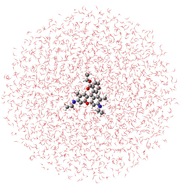
Figure 1: Schematic representation of the QM/FQ model.

The FQ FF can be effectively coupled to any QM method. It suffices to augment the QM energy functional with the classical functional in eq. (1) and the quantum/classical interaction. For the FQ FF the latter is defined as the classical electrostatic interaction between the FQs and the QM density.⁸⁰ Explicitly, the interaction takes the form:

$$E_{\mathrm{QM/FQ}}=\sum_{i=1}^{N_{\mathrm{FQ}}}V[\rho](\mathbf{r}_{i})q_{i}=\sum_{i=1}^{N_{\mathrm{FQ}}}\sum_{\mu,\nu=1}^{N_{\mathrm{AO}}}\Braket{\chi_{\mu}}{\frac{-q_{i}}{\left missing}{\mathbf{r}-\mathbf{r}_{i}\right|}|\chi_{\nu}}{D}_{\nu\mu},$$ (3)

with $V[\rho](\mathbf{r}_{i})$ the electrostatic potential due to the QM density of charge at the $i$-th FQ $q_{i}$ placed at $\mathbf{r}_{i}$, $\{\chi_{\mu}\}$ a Gaussian atomic orbital (AO) basis set and $D_{\mu\nu}$ the AO density matrix. For a hybrid Kohn–Sham (KS) DFT description of the QM moiety, the global QM/MM energy functional reads:^{80, 79}

$$\mathcal{E}[\bm{D},\bm{q},\bm{\bm{\lambda}}]=E_{\mathrm{SCF}}[\bm{D}]+F[\bm{q},\bm{\lambda}]+\bm{q}^{\dagger}\bm{V}(\bm{D}).$$ (4)

Stationarity of eq. (4) with respect to the density matrix yields the self-consistent field (SCF) equations:

$$\mathbf{F}\bm{C}=\bm{S}\bm{C}\bm{\epsilon},\quad\bm{F}=\bm{h}+\bm{G}^{\gamma}(\bm{D})+\bm{F}_{\mathrm{xc}}+\bm{F}_{\mathrm{FQ}}$$ (5)

where the various terms in the KS matrix $\bm{F}$ are:

$$h_{\mu\nu} =\Braket{\chi_{\mu}}{-\frac{1}{2}\nabla^{2}-\sum_{K}\frac{Z_{K}}{\left missing}{\bm{R}_{K}-\bm{r}\right|}|\chi_{\nu}}{\text{missing}}{,}$$ (6a)

$$G_{\mu\nu}^{\gamma}(\bm{D}) =\sum_{\alpha\beta}D_{\beta\alpha}(g_{\mu\nu\alpha\beta}-\gamma g_{\mu\beta\alpha\nu})\text{,}$$ (6b)

$$F_{\mathrm{xc},\mu\nu} =\int\mathop{}\!\mathrm{d}\bm{r}\chi_{\mu}(\bm{r})\chi_{\nu}(\bm{r})\left.\frac{\partial E_{\mathrm{xc}}}{\partial\rho(\bm{r})}\right|_{\rho(\bm{r})}=\int\mathop{}\!\mathrm{d}\bm{r}\chi_{\mu}(\bm{r})\chi_{\nu}(\bm{r})v_{\mathrm{xc}}(\bm{r})\text{,}$$ (6c)

$$F_{\mathrm{FQ},\mu\nu} =\bm{q}^{\dagger}\bm{V}_{\mu\nu}=\sum_{i=1}^{N_{\mathrm{FQ}}}\Braket{\chi_{\mu}}{\frac{-q_{i}}{\left missing}{\mathbf{r}-\mathbf{r}_{i}\right|}|\chi_{\nu}}{\text{missing}}{.}$$ (6d)

The FQs consistent with the QM density are obtained by solving the stationarity conditions with respect to the polarization variational degrees of freedom $\bm{q}$, i. e. by solving eq. (2) with a modified right-hand side (RHS), including the QM potential as additional source term, effectively coupling the QM and MM moieties and ensuring mutual polarization:

$$\begin{pmatrix}\bm{J}&\bm{1}_{\bm{\lambda}}\\ \bm{1}^{\dagger}_{\bm{\lambda}}&\bm{0}\\ \end{pmatrix}\begin{pmatrix}\bm{q}\\ \bm{\lambda}\end{pmatrix}=-\begin{pmatrix}\bm{\chi}+\bm{V}(\bm{D})\\ \bm{Q}\end{pmatrix}$$ (7)

.

2.1.1 Linear and Quadratic Response Functions in a QM/FQ framework

Thanks to its variational formalism, the QM/FQ approach⁷⁷ is especially suited to the modeling of response and spectral properties because its energy expression can be easily differentiated up to high orders. The quantum/classical coupling terms needed for the calculation of response properties, can be easily derived and implemented so that polarization effects are fully considered also in the computed final spectral data.^{80, 79, 103, 86, 87, 81, 104}

For a QM/FQ system subject to a Hermitian, time-periodic, one-electron perturbation $V^{t}$, response functions and response equations can be formulated in the atomic orbital, density matrix-based quasienergy formalism¹⁰⁵ of Thorvaldsen et al. ¹⁰⁶. To the best of our knowledge, this is the first time the quasienergy formalism is employed in the QM/FQ framework. The starting point is the time-averaged quasienergy Lagrangian, $\{\tilde{L}(\tilde{\bm{C}},\tilde{\bm{\mu}},\tilde{\bm{q}},t)\}_{T}$, parametrized in terms of the desired perturbed coefficient matrix $\tilde{\bm{C}}$, the Lagrange multipliers ensuring orthonormality of the one-electron basis $\tilde{\bm{\mu}}$ and the perturbed FQs $\tilde{\bm{q}}$. The tilde is here used for quantities evaluated at general perturbation strengths. We can obtain this Lagrangian by augmenting the quasienergy in eq. (52) of Ref. 106 with the perturbed FQ functional of eq. (1). The time-averaged quasienergy Lagrangian is not suitable for an atomic orbital-based theory, since it features the molecular orbital (MO) coefficient matrix. However, its perturbation-strength-differentiated counterpart $\{\tilde{L}^{a}(\tilde{\bm{D}},\tilde{\bm{q}},t)\}_{T}$ can be expressed in terms of the desired variational degrees of freedom $\tilde{\bm{D}}$ and $\tilde{\bm{q}}$:

$$\tilde{L}^{a}(\tilde{\bm{D}},\tilde{\bm{q}},t)\overset{\{\mathrm{Tr}\}_{T}}{=}\tilde{\mathcal{E}}^{00,a}-\tilde{\bm{S}}^{a}\tilde{\bm{W}},$$ (8)

where we have borrowed notation from Ref. 56. Indeed, the close similarity between the PCM and FQ models allows us to leverage the same arguments in Ref. 56 to formulate linear and quadratic response functions in a QM/FQ framework. The generalized KS energy $\tilde{\mathcal{E}}$ is the time-dependent equivalent of eq. (4):

$$\tilde{\mathcal{E}}[\tilde{\bm{D}},\tilde{\bm{q}}]\overset{\mathrm{Tr}}{=}\left[\tilde{\bm{h}}+\tilde{\bm{V}}^{t}+\frac{1}{2}\tilde{\bm{G}}^{\gamma}(\tilde{\bm{D}})-\frac{\mathrm{i}}{2}\tilde{\bm{T}}\right]\tilde{\bm{D}}+\tilde{E}_{\mathrm{xc}}[\tilde{\rho}(\tilde{\bm{D}})]+h_{\mathrm{nuc}}+F[\tilde{\bm{q}},\tilde{\bm{\lambda}}]+\tilde{\bm{q}}^{\dagger}\tilde{\bm{V}}(\tilde{\bm{D}})\text{.}$$ (9)

where $\tilde{\bm{V}}^{t}$ is the AO basis representation of the perturbation operator and $\tilde{\bm{T}}=\Braket{\tilde{\chi}_{\mu}}{\dot{\tilde{\chi}}_{\nu}}-\Braket{\dot{\tilde{\chi}}_{\mu}}{\tilde{\chi}_{\nu}}$ is the time-differentiation AO overlap matrix. Evaluation of eq. (8) at zero perturbation strength yields the the first-order property formula. For an electric field perturbation this corresponds to the electric dipole moment and, thanks to the Hellmann–Feynman theorem, only requires the unperturbed density matrix. Further differentiation of eq. (8) and evaluation at zero perturbation strength yields higher order response functions. Detailed expressions can be obtained from eqs. (22a)-(22c) and Appendix A in Ref. 56 by replacing perturbed and unperturbed apparent surface charges $\sigma$ with perturbed and unperturbed FQs, respectively and the generalized free energy $\mathcal{G}$ with $\mathcal{E}$:

$$L^{ab}\overset{\{\mathrm{Tr}\}_{T}}{=} \mathcal{E}^{00,ab}+\mathcal{E}^{10,a}\bm{D}^{b}+\mathcal{E}^{01,a}\bm{q}^{b}-\bm{S}^{ab}\bm{W}-\bm{S}^{a}\bm{W}^{b}$$ (10a)

$$\begin{split}L^{abc}\overset{\{\mathrm{Tr}\}_{T}}{=}&\mathcal{E}^{00,abc}+\mathcal{E}^{10,ac}\bm{D}^{b}+\mathcal{E}^{10,ab}\bm{D}^{c}+\mathcal{E}^{20,a}\bm{D}^{b}\bm{D}^{c}+\mathcal{E}^{10,a}\bm{D}^{bc}+\mathcal{E}^{11,a}\bm{D}^{b}\bm{q}^{c}\\ &+\mathcal{E}^{01,ac}\bm{q}^{b}+\mathcal{E}^{01,ab}\bm{q}^{c}+\mathcal{E}^{01,a}\bm{q}^{bc}+\mathcal{E}^{11,a}\bm{q}^{b}\bm{D}^{c}\\ &-\bm{S}^{abc}\bm{W}-\bm{S}^{ab}\bm{W}^{c}-\bm{S}^{ac}\bm{W}^{b}-\bm{S}^{a}\bm{W}^{bc}\end{split}$$ (10b)

Response parameters need to be determined in order to assemble the property expressions from the perturbed variational parameters $\bm{D}^{a}$, $\bm{q}^{a}$ and so forth appearing in the expressions given above. Zero-field perturbation-strength differentiation of the orthonormality, TDSCF, and FQ equations yields the desired response equations.^{106, 107, 56} Solution of the $N$-th order response equations for the $b_{\mathrm{N}}$ perturbation tuple yields the desired response parameters $\bm{X}^{b_{N}}$. The perturbed variational parameters are further partitioned into a sum of homogeneous and particular contributions.¹⁰⁶ Whereas the former depend on the $N$-th order response parameters, the latter depend only on lower order response parameters. With this partition, the response equations to any order can be compactly rearranged as:^{108, 109}

$$\left[\bm{E}^{[2]}-\omega_{b_{N}}\bm{S}^{[2]}\right]\bm{X}^{b_{N}}=\bm{M}_{\mathrm{RHS}}^{b_{N}}.$$ (11)

The left-hand side (LHS) includes the generalized Hessian and metric matrices, $\bm{E}^{[2]}$ and $\bm{S}^{[2]}$, respectively and $\omega_{b_{N}}=\sum_{i=1}^{N}\omega_{b_{i}}$. The RHS $\bm{M}_{\mathrm{RHS}}^{b_{N}}$ collects contributions from lower-order perturbed density matrices and $N$-th order particular contributions, see Refs. 106, 107, 56.

For a single, electric-field type perturbation, the matrix-vector products $\bm{E}^{[2]}\bm{X}^{b}$ and $\bm{S}^{[2]}\bm{X}^{b}$ assume the form:

$$\bm{E}^{[2]}\bm{X}^{b} =\bm{G}^{\mathrm{KS}}([\bm{X}^{b},\bm{D}]_{\bm{S}})\bm{D}\bm{S}-\bm{S}\bm{D}\bm{G}^{\mathrm{KS}}([\bm{X}^{b},\bm{D}]_{\bm{S}})+\bm{F}[\bm{X}^{b},\bm{D}]_{\bm{S}}\bm{S}$$

$$-\bm{S}[\bm{X}^{b},\bm{D}]_{\bm{S}}\bm{F}+\bm{q}_{\mathrm{H}}^{b}\bm{V}\bm{D}\bm{S}-\bm{S}\bm{D}\bm{V}\bm{q}^{b}_{\mathrm{H}}$$ (12)

$$\bm{S}^{[2]}\bm{X}^{b} =\bm{S}[\bm{X}^{b},\bm{D}]_{\bm{S}}\bm{S}\text{.}$$ (13)

where $\bm{G}^{\mathrm{KS}}$ now collects the two-electron and exchange-correlation contributions. The general expression for the RHS (see eq. (46) in Ref. 56) simplifies to the matrix elements of the electric dipole perturbation operator, with no contributions from the classical polarizable model. These equations are equivalent, upon transformation to the MO basis, to their more familiar formulation as Casida’s equations.^{110, 80} Perturbed FQs are obtained by solving:

$$\bm{J}\bm{q}^{b}_{\mathrm{H}}=-\bm{V}(\bm{D}^{b}_{\mathrm{H}}),$$ (14)

once again highlighting the introduction of the mutual QM/MM polarization.

Response equations for the second-order response parameters $\bm{X}^{bc}$ can be derived in a similar fashion. Restricting ourselves to electric-field type perturbations only, the linear transformations are expressed as:

$$\bm{E}^{[2]}\bm{X}^{bc} =\bm{G}^{\mathrm{KS}}([\bm{X}^{bc},\bm{D}]_{\bm{S}})\bm{D}\bm{S}-\bm{S}\bm{D}\bm{G}^{\mathrm{KS}}([\bm{X}^{bc},\bm{D}]_{\bm{S}})+\bm{F}[\bm{X}^{bc},\bm{D}]_{\bm{S}}\bm{S}$$

$$-\bm{S}[\bm{X}^{bc},\bm{D}]_{\bm{S}}\bm{F}+\bm{q}_{\mathrm{H}}^{bc}\bm{V}\bm{D}\bm{S}-\bm{S}\bm{D}\bm{V}\bm{q}^{bc}_{\mathrm{H}}$$ (15)

$$\bm{S}^{[2]}\bm{X}^{bc} =\bm{S}[\bm{X}^{bc},\bm{D}]_{\bm{S}}\bm{S}\text{.}$$ (16)

In contrast to the linear response equations, the RHS will contain FQ contributions:

$$\bm{M}_{\mathrm{RHS,FQ}}^{bc}=\left[(\bm{q}^{bc}_{\mathrm{P}})^{\dagger}\bm{V}\bm{D}\bm{S}+\bm{q}^{\dagger}\bm{V}\bm{D}_{\mathrm{P}}^{bc}\bm{S}+(\bm{q}^{b}_{\mathrm{H}})^{\dagger}\bm{V}\bm{D}^{c}_{\omega}\bm{S}+(\bm{q}^{c}_{\mathrm{H}})^{\dagger}\bm{V}\bm{D}^{b}_{\omega}\bm{S}\right]^{\ominus},$$ (17)

with the second-order particular FQs calculated as the solution to the linear equation:

$$\bm{J}\bm{q}^{bc}_{\mathrm{P}}=-\bm{V}(\bm{D}^{bc}_{\mathrm{P}}),$$ (18)

and the perturbed density matrix $\bm{D}^{bc}_{\mathrm{P}}$ is in turn assembled from first-order perturbed density matrices.

As for the PCM, there are two classes of contributions from the classical polarizable region: implicit, through the unperturbed Fock matrix, and explicit, through the $N$-th order perturbed homogeneous FQs. This is indeed a trait shared by any quantum/classical polarizable model.

2.1.2 One- and Two-Photon Absorption

We can formulate one- and two-photon absorption parameters in terms of single residues of the linear and quadratic response functions, respectively. Friese et al. ¹¹¹ have presented a density matrix-based, open-ended formulation of single residues that can be coupled to classical polarizable models.^{90, 56}

TPA cross sections of randomly oriented systems can be calculated from the imaginary part of the third susceptibility. Alternatively, they can be obtained as the individual two-photon transition matrix elements $S_{ab}$ between the initial state $\ket{i}$ and final state $\ket{f}$, with the sum-over-states expression:¹¹²

$$S_{ab}=\sum_{s}\left(\frac{\braket{i}{\mu_{a}}{s}\braket{s}{\mu_{b}}{f}}{\omega_{si}-\omega}+\frac{\braket{i}{\mu_{b}}{s}\braket{s}{\mu_{a}}{f}}{\omega_{si}-\omega}\right)$$ (19)

where $a,b\in x,y,z$ and $\omega$ is the frequency of the external radiation, which is half of the excitation energy $\omega_{f}$ to the final state $\ket{f}$ ($2\omega=\omega_{f}$). The summation runs over all $s$ states, including initial and final state. $\omega_{si}=\omega_{s}-\omega_{i}$ is the transition energy between $s$ and $i$ states.

For linearly polarized light with parallel polarization, rotationally averaged microscopic OPA and TPA cross sections can be written in terms of the transition matrix tensors $\mathbf{S}$ and their complex conjugates $\mathbf{\overline{S}}$ as:

$$\langle\delta^{\rm 1PA}\rangle =\frac{1}{3}\sum_{a}S_{a}\bar{S}_{a}$$ (20)

$$\langle\delta^{\rm 2PA}\rangle =\frac{1}{15}\sum_{ab}\left(2S_{ab}\bar{S}_{ab}+S_{aa}\bar{S}_{bb}\right).$$ (21)

Finally, the macroscopic TPA cross section in cgs units can be obtained from the rotationally averaged TPA strengths ($\braket{\delta^{\text{TPA}}}$) expressed in atomic units as:

$$\sigma^{\text{TPA}}=\frac{N\pi^{3}\alpha a^{5}_{0}\omega^{2}}{c}\braket{\delta^{\text{TPA}}}g(2\omega,\omega_{0},\Gamma)$$ (22)

where $N=4$ in case of single beam experiments, $\alpha$ is the fine structure constant, $a_{0}$ is the Bohr radius, $\omega$ is the photon energy in atomic units, $c$ is the speed of light and $g(2\omega,\omega_{0},\Gamma)$ the lineshape function describing spectral broadening effects. The common unit for TPA cross sections is GM in honour of the work of Maria Goppert-Mayer (1 GM = 10^-50 cm⁴ s photon^-1). We refer the reader to Ref. 10 for further details on the computational approach to TPA cross sections.

2.2 Implementation

The close similarity of the PCM and FQ models renders the implementation of the latter a rather straightforward extension of the former. Our implementation relies on the PCMSolver library,¹¹³ which already provides the infrastructure for the PCM and lends itself to the extensions needed for a FQ implementation. The calculation of TPA cross sections with the FQ discrete model was implemented in the LSDALTON program package.¹¹⁴ LSDALTON provides single residues of the quadratic response function in vacuo and we exploited the existing interface with PCMSolver¹¹⁵ to extend this functionality to include the PCM and FQ quantum/classical polarizable models. The TPA implementation in LSDALTON leverages the $2n+1$ rule. Ensuring correctness of the linear response calculations is enough to guarantee correctness up to cubic response properties. We performed extensive testing of the PCM and FQ linear and quadratic response functions, including their residues, against DALTON.^{53, 54, 55, 14}

The use of a modular programming paradigm, based on open-source libraries and programs, is particularly beneficial for the work here presented. The most significant programming investment was the extension of the PCMSolver library.

3 Computational Details

Rhodamine 6G (R6G) (see Figure 2) in aqueous solution has been amply studied experimentally using both OPA and TPA techniques.^{91, 92, 93, 94, 95, 96, 97, 16} Such a system is capable of forming solute-solvent hydrogen bonds, and is thus a good test case for our atomistic polarizable QM/FQ approach.

We adopted the following computational protocol for our QM/MM calculations of excitation energies, OPA and TPA intensities:

Definition of the systems and calculation of atomic charges

The solute molecule was surrounded by a number of water molecules large enough to represent all the solute-solvent interactions (at least 8500). The atomic charges of the solute were computed by using the Charge Model 5 (CM5).¹¹⁶

Classical MD simulations in aqueous solution

The MD simulations were performed in a cubic box reproduced periodically in every direction, satisfying periodic boundary conditions (PBC). A minimization step ensures that simulations were started from a minimum of the classical PES. From the MD run, a set of snapshots was extracted to be used in the following QM/TIP3P⁹⁸ and QM/FQ calculations.

Definition of the different regions of the two-layer scheme and their boundaries

Each snapshot extracted from the MD run was cut into a sphere centered on the solute. A radius of 25 Å  was chosen in order to include all specific water-solute interactions.

QM/classical calculations

QM/TIP3P, and QM/FQ OPA and TPA calculations were performed on 100 structures obtained in the previous step. The results obtained for each spherical snapshot were extracted and averaged to produce the final value.

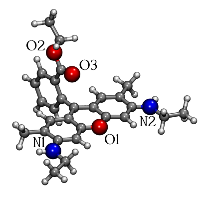
Figure 2: Rhodamine 6G structure and atom labeling.

In step 1, R6G was optimized and CM5 charges were calculated at the B3LYP/6-31+G* level of theory including solvent effects by means of the PCM ³².

The MD simulation was performed using GROMACS¹¹⁷, with the OPLS-AA ¹¹⁸ force fields to describe intra- and inter-molecular interactions. CM5 charges were used to account for electrostatic interactions. The TIP3P FF was used to describe the water molecules ⁹⁸. A single molecule was dissolved in a cubic box containing at least 8500 water molecules. A chloride ion has been included in the box to neutralize the system. The chromophore was kept fixed during all the steps of the MD run. This neglects geometric relaxation due to solvation and is an approximation. However, our primary goal is to compare direct (electronic) rather than indirect (geometrical) solvent effects on the properties. Furthermore, this approximation affords a fairer comparison with implicit solvent models. R6G in aqueous solution was initially brought to 0 K with the steepest descent minimization procedure and then heated to 298.15 K in an NVT ensemble using the velocity-rescaling¹¹⁹ method with an integration time step of 0.2 fs and a coupling constant of 0.1 ps for 200 ps. The time step and temperature coupling constant were then increased to 2.0 fs and 0.2 ps, respectively, and an NPT simulation (using the Berendsen barostat and a coupling constant of 1.0 ps) for 1 ns was performed to obtain a uniform distribution of molecules in the box. A 10 ns production run in the NVT ensemble was then carried out, fixing the fastest internal degrees of freedom by means of the LINCS algorithm ($\delta$t=2.0 fs)¹²⁰, and freezing the R6G at the center of the simulation box. Electrostatic interactions are treated by using particle-mesh Ewald (PME) ¹²¹ method with a grid spacing of 1.2 Å and a spline interpolation of order 4. We have excluded intramolecular interactions between atom pairs separated up to three bonds. A snapshot every 100 ps was extracted in order to obtain a total of 100 uncorrelated snapshots.

For each snapshot a solute-centered sphere with a radius of 25 Å was cut. Notice that the chloride ion was not present in any of the extracted spherical snapshots. For each snapshot, OPA and TPA spectra were then calculated with two QM/MM approaches: the water molecules were modeled by means of the non-polarizable TIP3P FF,⁹⁸ and the FQ SPC parametrization proposed by Rick et al. ⁷⁵. For comparison, we also ran QM calculations on the isolated chromophore and embedded in a PCM continuum modelling the water solution.

We performed all OPA calculations using a locally modified version of the Gaussian 16 package,¹²² whereas we used a locally modified version of the LSDALTON program,¹¹⁴ interfaced to the PCMSolver library,¹¹³ for the TPA calculations. The CAM-B3LYP/6-31+G* model chemistry was used in all calculations. For the LSDALTON calculations we leveraged the implementation of density fitting, with the df-def2 auxiliary fitting basis, to accelerate the evaluation of the Coulomb matrix.

For the PCM calculations, the cavity was generated from a set of atom-centered, interlocking spheres. PCMSolver implements the GePol algorithm for cavity generation and uses the Bondi–Mantina set of van der Waals radii ^{123, 124} 1.20 Å for hydrogen, 1.70 Å for carbon, 1.55 Å for nitrogen and 1.52 Å for oxygen. All radii were scaled by a factor of 1.2. Values of the static and optical permittivities of $\varepsilon_{\mathrm{s}}=78.39$ and $\varepsilon_{\infty}=1.776$, respectively, were used for the PCM calculations in water in LSDALTON.

For the PCM calculations in Gaussian, the following atomic radii were used and scaled by a factor of 1.1: 1.443 Å for hydrogen, 1.9255 Å for carbon, 1.83 Å for nitrogen and 1.75 Å for oxygen. Values of the static and optical permittivities of $\varepsilon_{\mathrm{s}}=78.3553$ and $\varepsilon_{\infty}=1.77785$, respectively, were instead used to model water solvent effects.

The differences in PCM parametrization between the two codes used in this study did not lead to significant differences (less than 1%) between computed ground state energies, excitation frequencies and oscillator strengths.

4 Numerical Results

First, we analyze the MD runs in terms of the hydration patterns with a particular focus on hydrogen bonds (HBs) formed between R6G and solvent water molecules. Second, OPA and TPA spectra are presented and compared with their experimental counterparts.

4.1 MD analysis: Hydration Pattern

R6G is characterized by a keto oxygen and by amino groups, which can act as HB donors, whereas the ether oxygen atoms (O1 and O2) together with the amino nitrogen atoms (N1 and N2) can act as HB acceptors (see Figure 2 for atom labeling). HB patterns were analyzed by extracting the radial distribution functions $g(r)$ from the MD trajectories. For this analysis the TRAVIS package was used.¹²⁵ The radial distribution functions were computed taking as reference oxygen atoms (O1, O2 and O3), nitrogen atoms (N1 and N2) and amino hydrogen atoms (H1 and H2) of the solute; they are plotted in Figure 3. The most intense peak of the $g(r)$ refers to the carboxylic oxygen (O3), whereas the other atoms are not involved in HBs with the solvent water molecules. The average number of HBs between water molecules and the carboxylic oxygen (O3) is 1.7, thus confirming strong HB patterns.

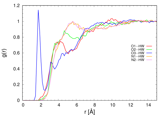
Figure 3: Radial distribution function $g(r)$ between selected sites of R6G and water molecules. The considered atomic sites are highlighted in Figure 2

4.2 OPA Spectra of R6G in aqueous solution

100 uncorrelated snapshots were extracted from the MD run. The convergence of the studied properties (OPA and TPA spectra) was checked by considering an increasing number of snapshots. These results are reported in Figures S1 and S2 in the supporting information (SI).

QM/FQ OPA results are depicted in Figure 4. Raw data (sticks) and their Gaussian convolution, with full width at half maximum (FWHM) of 0.1 eV, are shown.

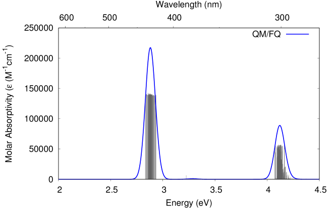
Figure 4: QM/FQ calculated OPA spectrum of R6G in aqueous solution reported as stick spectrum and convoluted with a Gaussian band shape (FWHM=0.1 eV)

The OPA spectrum is characterized by an intense transition (S1) at about 2.8 eV (440 nm) which is related to a pure HOMO$\rightarrow$LUMO transition. The second transition (S2) is a pure HOMO-1$\rightarrow$LUMO transition and is located at about 3.2 eV (380 nm). This transition is dark due to the symmetry of the involved orbitals, see Figure 5. Our findings confirm what already reported in previous theoretical studies,⁹² and is in contrast with some experimental works,¹⁶ where S2 is instead assigned to a visible transition. The third transition predicted by the QM/FQ approach is located at 4.1 eV (300 nm), and involves a combined transition between HOMO-1$\rightarrow$LUMO+1 and HOMO-2$\rightarrow$LUMO. The whole computed spectrum, involving also the higher transitions, is reported in the SI ( Figure S3).

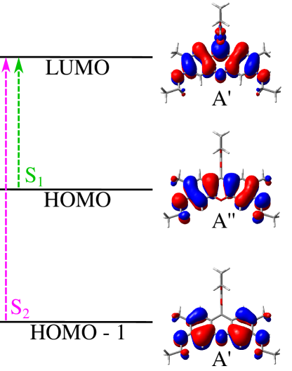
Figure 5: Graphical scheme of the first two transitions of R6G in aqueous solution. Molecular orbitals related to each transition are depicted.

We investigated the relevance of solvent effects by employing different computational approaches, ranging from continuum QM/PCM to nonpolarizable QM/TIP3P and polarizable QM/FQ descriptions. As a reference, the OPA spectrum of the solute in vacuo was also calculated. Vertical excitations and oscillator strengths as obtained by exploiting the different approaches summarized in Table 1 and graphically depicted in Figure 6. The experimental spectrum is also reported.¹⁶

Table 1: Vacuum and aqueous solution vertical excitation energies (eV) and oscillator strengths (a.u.) for the three lowest singlet excited states of R6G calculated at the CAM-B3LYP/6-31+G* level of theory. QM/PCM, QM/TIP3P and QM/FQ approaches were used to model environment effects in solution. The experimental vertical excitation energies are also reported.

	Vacuum		QM/PCM		QM/TIP3P		QM/FQ		Exp.$\phantom{t}{}^{\text{a}}$
	$E_{\text{vert}}$	$f$	$E_{\text{vert}}$	$f$	$E_{\text{vert}}$	$f$	$E_{\text{vert}}$	$f$	$E_{\text{vert}}$
S1	$3.07$	$0.89$	$2.98$	$1.05$	$2.82$	$0.84$	$2.81$	$0.90$	$2.27$
S2	$3.68$	$0.00$	$3.71$	$0.00$	$3.18$	$0.01$	$3.20$	$0.00$
S3	$4.42$	$0.25$	$4.47$	$0.29$	$4.15$	$0.21$	$4.13$	$0.26$	$3.46$

$\phantom{t}{}^{\text{a}}$ Experimental values are taken from Ref. 16.

The experimental spectrum is dominated by an intense transition (S1) at about 2.3 eV (550 nm), characterized by an inhomogeneous band broadening, probably due to a vibronic convolution. The second visible transition is instead at about 3.6 eV (350 nm) and can be associated to the S3 transition.

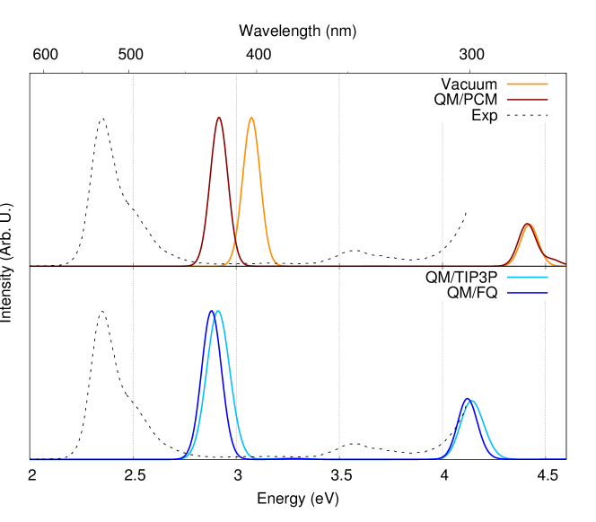
Figure 6: One-photon absorption spectra for the R6G chromophore at the CAM-B3LYP/6-31+G* level of theory. Computed vacuum, QM/PCM, QM/TIP3P and QM/FQ OPA spectra are reported. The experimental spectrum is reproduced from Ref. 16.

The first transition (S1) is predicted to be the most intense by all the different methods, with a redshift when solvent effects are taken into consideration. In particular, QM/PCM, QM/TIP3P and QM/FQ predict very similar vertical excitation energies for the S1 transition, with the largest redshift shown by QM/FQ. All the approaches considered correctly describe the S2 transition as being symmetry-forbidden, see Table 1. The models employed exhibit major differences for the third transition (S3), which is predicted at about 280 nm in vacuum and by QM/PCM, and at about 310 nm by both QM/TIP3P and QM/FQ approaches (see Fig.6). The atomistic description captures the explicit solvent-solute interactions that appear to be crucial in the modeling of this transition. Implicit solvation is unable to capture solvent effects, as it is shown by the negligible differences observed with respect to the vacuum results. Furthermore, the energy difference between S1 and S3 is correctly predicted by QM/MM approaches ($\sim 1.18$ eV) as compared to the experimental value (1.19 eV), whereas it is overestimated by the QM/PCM approach (1.49 eV). Notice also that by considering energy differences, instead of absolute vertical excitation energies, systematic errors and biases due to the choice of QM method, and in particular of a specific DFT functional, should be avoided.

To further analyze the nature of the electronic transitions, their charge transfer (CT) nature was characterized by a simple index, denoted as $D_{\mathrm{CT}}$.^{126, 127} The barycenters of the positive and negative density distributions are calculated as the difference of ground state (GS) and excited state (ES) densities. The CT length index ($D_{\mathrm{CT}}$ ) is defined as the distance between the two barycenters. Calculated vacuum, QM/PCM, QM/TIP3P and QM/FQ $D_{\mathrm{CT}}$ values are reported in Table 2.

Table 2: $D_{\mathrm{CT}}$ indices (Å) for the first three excited states as obtained by exploiting the various models considered in this work.

	Vacuum	QM/PCM	QM/TIP3P	QM/FQ
S1	$1.195$	$1.170$	$1.668$	$1.624$
S2	$1.318$	$1.336$	$1.587$	$1.574$
S3	$0.811$	$0.759$	$4.043$	$3.580$

The first two transitions (S1 and S2) have little CT character. The largest difference between the considered approaches is shown by the S3 transition, of which the CT character is irrelevant in vacuo and at the QM/PCM level, whereas is huge at both QM/TIP3P and QM/FQ levels. This different behaviour was expected by considering the computed OPA spectra reported in Figure 6; in fact, the largest discrepancy between vacumm-QM/PCM and QM/MM approaches was indeed predicted for the S3 transition.

4.3 TPA Spectra of R6G in aqueous solution

Figure 7 reports computed QM/FQ TPA raw data and their Gaussian convolution. We adopted a Gaussian lineshape with FWHM of 0.1 eV in agreement with previous computational studies on TPA and suggested best practices, see Ref. 10.

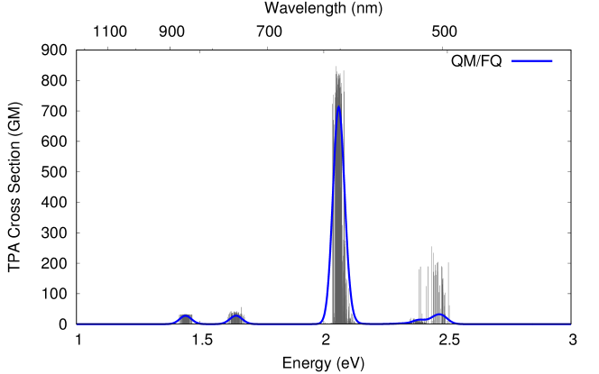
Figure 7: QM/FQ calculated TPA spectrum of R6G in aqueous solution reported as stick spectrum and convoluted with a Gaussian band shape (FWHM = 0.1 eV)

The first two visible transitions at about 1.4 and 1.6 eV have almost the same intensity and they are the S1 and S2 transitions, respectively. The S2 transition is not dark, due to the different symmetry selection rules in TPA compared to OPA (see Figure 4). The computed QM/FQ TPA spectrum is dominated by an intense peak at about 2.06 eV (600 nm) associated to the S3 transition.

We compared different approaches to model solvent effects also for TPA spectra and considered QM/PCM, QM/TIP3P and QM/FQ models. In addition, TPA spectra of R6G in vacuo was computed as an additional reference point. Vacuum, QM/PCM, QM/TIP3P and QM/FQ TPA spectra are plotted in Figure 8 together with the experimental spectrum, reproduced from Ref. 91.

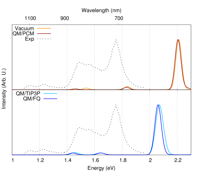
Figure 8: Two-photon absorption spectra for the R6G chromophore at the CAM- B3LYP/6-31+G* level of theory. Computed vacuum, QM/PCM, QM/TIP3P and QM/FQ OPA spectra are reported. The experimental spectrum is reproduced from Ref. 91.

The experimental TPA spectrum is characterized by three main peaks at 1.14, 1.52, and 1.73 eV. These correspond to the S1, S2 and S3 transitions, respectively. It is worth noting that the peak at about 1.25 eV was wrongly reported to be associated to the S2 transition in some experimental works due to the similar intensity with respect to the peak at 1.14 eV.¹⁶ Milojevich et al. recently showed that such a peak is instead a vibronic band due to Herzberg–Teller terms.⁹² Notice in fact that such a vibronic peak exactly corresponds to the vibronic peak present also in the experimental OPA spectrum, see Figure 6. In this work, we are not considering any vibronic contributions because our main goal is to show the performance of QM/FQ approach in predicting solvent effects on multiphoton spectroscopies. As a consequence, the peak at 1.25 eV cannot be reproduced by the different approaches explored in this work.

The computed vacuum and aqueous solution transition energies and TPA cross sections (in GM units) of the first three transitions are reported in Table 3, together with their experimental values. It is clear from Figure 8 and Table 3 that all the approaches considered in this work predict the S3 transition as the most intense in the TPA spectrum. The whole TPA spectra, including also higher energy transitions, are reported in Figure S4 of the SI.

Table 3: Vacuum and aqueous solution TPA vertical excitation energies (eV) and cross sections (GM) for the six lowest singlet excited states of R6G calculated at the CAM-B3LYP/6-31+G* level of theory. QM/PCM, QM/TIP3P and QM/FQ approaches were used to model environment effects in aqueous solution. The experimental TPA vertical excitation energies and cross sections are also reported.

	Vacuum		QM/PCM		QM/TIP3P		QM/FQ		Exp.$\phantom{t}{}^{\text{a}}$
	$E_{\text{TPA}}$	$\sigma$	$E_{\text{TPA}}$	$\sigma$	$E_{\text{TPA}}$	$\sigma$	$E_{\text{TPA}}$	$\sigma$	$E_{\text{TPA}}$	$\sigma$
S1	$1.54$	$15.52$	$1.46$	$24.03$	$1.46$	$18.67$	$1.44$	$27.37$	$1.14$	$15$
S2	$1.84$	$29.83$	$1.83$	$69.55$	$1.64$	$16.92$	$1.64$	$27.59$	$1.52$	$65$
S3	$2.21$	$466.50$	$2.20$	$1390.33$	$2.07$	$417.39$	$2.06$	$712.69$	$1.73$	$150$

$\phantom{t}{}^{\text{a}}$ Experimental values from Ref. 91.

Both QM/MM approaches outperform the vacuum and QM/PCM models in reproducing the experimental relative differences between the vertical transition energies. As already pointed out in case of OPA spectra (see Figure 6 and Table 1), this is particularly evident in the case of the S1-S3 difference. The relative intensity of the S1 and S3 transitions is correctly reproduced by all the different methods, with the best agreement with experiment shown by QM/TIP3P and QM/FQ.

The largest discrepancy is reported in case of the S2 transition for both relative energies and intensities. The data reported in Table 3 show that the S1-S2 energy difference is indeed wrongly reproduced even by QM/MM approaches ($\sim$ 0.2 eV vs. 0.38 eV in the experiment). Some differences between the considered methods are encountered in case of relative intensities between S1 and S2. In particular, QM/PCM is almost able to reproduce the experimental intensity ratio between the two peaks (2.9 vs. 4.3), whereas non-polarizable QM/TIP3P results are the worst (0.9 vs. 4.3). Such a huge discrepancies probably reflects the fact that for this transition, HB interactions play a minor role with respect to polarization effects.

Finally, the major effect of including polarization effects in the description of solvent effects is the increase of the S3 TPA cross section, which is reported by both QM/PCM and QM/FQ whereas QM/TIP3P is consistent with the vacuum counterpart. Remarkably, in passing from a continuum to a discrete approach (QM/FQ), the S3 TPA cross section decreases, thus moving closer to the experimental value.

To conclude our comparison between computed and experimental TPA spectra of R6G in water, it is worth pointing out that experimental TPA measurements are not a standard technique.⁹¹ In fact, as reported in Figure S5 in the SI, several experimental TPA spectra of R6G in aqueous solution have been reported previously in the literature,⁹¹ showing large discrepancies even in the measured spectra. Therefore, a quantitative comparison is particularly challenging.

5 Summary, Conclusions and Perspectives

In this paper, the extension of the QM/FQ approach to linear and quadratic response in the quasienergy formalism has been presented for the first time. The approach has been coupled to a classical MD simulation in order to have a reliable sampling of the phase space. The computational protocol has been applied to a challenging problem, i. e. the OPA and TPA spectra of R6G in aqueous solution. Such a molecule is characterized by a transition (S2) that is dark in OPA spectra due to symmetry selection rules, see Figure 6. Thanks to the different selection rules, however, such a transition is visible in TPA spectra, see Figure 8.

To analyze the importance of solvent effects for such a system, three different approaches have been considered, from a continuum (QM/PCM) to two QM/MM approaches (i. e. nonpolarizable QM/TIP3P and polarizable QM/FQ). Both QM/TIP3P and QM/FQ simulated OPA and TPA spectra show that the inclusion of discrete water solvent molecules is essential to increase the agreement between theory and experiment. However, some discrepancies still remain and are principally related to the OPA-dark S2 transition. For this particular transition, polarization effects included by both QM/PCM and QM/FQ seem to be crucial. Although the agreement with experiment increases by including solvent polarization, it still remains poor. This can be ascribed to several factors. The choice of DFT as the quantum mechanical methodology has been recently reported to systematically underestimate TPA cross sections if compared to reference resolution-of-the-identity CC2 data.²⁶ DFT functionals are mostly tested on vertical excitation energies, and only rarely on TPA cross sections, which for an OPA-dark transition is particularly problematic. In addition, as pointed out in Ref. 92, the inclusion of vibronic coupling can play an important role in the determination of TPA cross sections.^{128, 129} Finally, our polarizable QM/FQ approach models the interaction between the QM and MM portions in terms of electrostatic interactions only. Some of the present authors have recently developed different approaches to include non-electrostatic energy terms in QM/MM approaches,^{130, 131, 132} which can play a relevant role in predicting both OPA and TPA spectra.

RDR thanks Filippo Lipparini (Università di Pisa) for the enlightening discussions on the variational formulation of polarizable QM/classical models, and Simen S. Reine (Hylleraas Centre for Quantum Molecular Sciences, University of Oslo) for help in the parallel set up of the calculations presented in this work.

RDR and LF acknowledge the support of the Research Council of Norway through its Centres of Excellence scheme, project number 262695 and the Norwegian Supercomputer Program through a grant for computer time (Grant No. NN4654K). RDR also acknowledges support by the Research Council of Norway through its Mobility Grant scheme, project number 261873.

CC gratefully acknowledges the support of H2020-MSCA-ITN-2017 European Training Network “Computational Spectroscopy In Natural sciences and Engineering” (COSINE), grant number 765739.

Analysis of the convergence of the QM/FQ OPA and TPA spectra as a function of the number of snapshots. Calculated OPA and TPA spectra in the whole energy range. Experimental TPA spectra.

Input and output files for the LSDALTON calculations reported in this work are available on the Norwegian instance of the Dataverse data repository: https://doi.org/10.18710/C9OZWV.

References

- He et al. 2008 He, G. S.; Tan, L.-S.; Zheng, Q.; Prasad, P. N. Multiphoton absorbing materials: molecular designs, characterizations, and applications. Chem. Rev. 2008, 108, 1245–1330
- Göppert-Mayer 1931 Göppert-Mayer, M. Über elementarakte mit zwei quantensprüngen. Ann. Phys-Berlin 1931, 401, 273–294
- Kaiser and Garrett 1961 Kaiser, W.; Garrett, C. Two-photon excitation in Ca F 2: Eu 2+. Phys. Rev. Lett. 1961, 7, 229
- Terenziani et al. 2008 Terenziani, F.; Katan, C.; Badaeva, E.; Tretiak, S.; Blanchard-Desce, M. Enhanced two-photon absorption of organic chromophores: theoretical and experimental assessments. Adv. Mater. 2008, 20, 4641–4678
- Pawlicki et al. 2009 Pawlicki, M.; Collins, H. A.; Denning, R. G.; Anderson, H. L. Two-photon absorption and the design of two-photon dyes. Angew. Chem. Int. Ed. 2009, 48, 3244–3266
- Parthenopoulos and Rentzepis 1989 Parthenopoulos, D. A.; Rentzepis, P. M. Three-dimensional optical storage memory. Science 1989, 245, 843–845
- Gorman et al. 2004 Gorman, A.; Killoran, J.; O’Shea, C.; Kenna, T.; Gallagher, W. M.; O’Shea, D. F. In vitro demonstration of the heavy-atom effect for photodynamic therapy. J. Am. Chem. Soc. 2004, 126, 10619–10631
- Köhler et al. 1997 Köhler, R. H.; Cao, J.; Zipfel, W. R.; Webb, W. W.; Hanson, M. R. Exchange of protein molecules through connections between higher plant plastids. Science 1997, 276, 2039–2042
- Belfield et al. 2000 Belfield, K. D.; Ren, X.; Van Stryland, E. W.; Hagan, D. J.; Dubikovsky, V.; Miesak, E. J. Near-IR two-photon photoinitiated polymerization using a fluorone/amine initiating system. J. Am. Chem. Soc. 2000, 122, 1217–1218
- Beerepoot et al. 2015 Beerepoot, M. T.; Friese, D. H.; List, N. H.; Kongsted, J.; Ruud, K. Benchmarking two-photon absorption cross sections: performance of CC2 and CAM-B3LYP. Phys. Chem. Chem. Phys. 2015, 17, 19306–19314
- Friese et al. 2012 Friese, D. H.; Hättig, C.; Ruud, K. Calculation of two-photon absorption strengths with the approximate coupled cluster singles and doubles model CC2 using the resolution-of-identity approximation. Phys. Chem. Chem. Phys. 2012, 14, 1175–1184
- Guillaume et al. 2010 Guillaume, M.; Ruud, K.; Rizzo, A.; Monti, S.; Lin, Z.; Xu, X. Computational study of the one-and two-photon absorption and circular dichroism of (L)-tryptophan. J. Phys. Chem. B 2010, 114, 6500–6512
- Toro et al. 2010 Toro, C.; De Boni, L.; Lin, N.; Santoro, F.; Rizzo, A.; Hernandez, F. E. Two-Photon Absorption Circular Dichroism: A New Twist in Nonlinear Spectroscopy. Chem–Eur. J. 2010, 16, 3504–3509
- Ferrighi et al. 2007 Ferrighi, L.; Frediani, L.; Fossgaard, E.; Ruud, K. Two-photon absorption of [2.2] paracyclophane derivatives in solution: A theoretical investigation. J. Chem. Phys. 2007, 127, 244103
- Steindal et al. 2012 Steindal, A. H.; Olsen, J. M. H.; Ruud, K.; Frediani, L.; Kongsted, J. A combined quantum mechanics/molecular mechanics study of the one-and two-photon absorption in the green fluorescent protein. Phys. Chem. Chem. Phys. 2012, 14, 5440–5451
- Nag and Goswami 2009 Nag, A.; Goswami, D. Solvent effect on two-photon absorption and fluorescence of rhodamine dyes. J. Photoch. Photobio. A 2009, 206, 188–197
- Paterson et al. 2006 Paterson, M. J.; Christiansen, O.; Pawłowski, F.; Jørgensen, P.; Hättig, C.; Helgaker, T.; Sałek, P. Benchmarking two-photon absorption with CC3 quadratic response theory, and comparison with density-functional response theory. J. Chem. Phys 2006, 054322
- Hattig et al. 1998 Hattig, C.; Christiansen, O.; Jorgensen, P. Multiphoton transition moments and absorption cross sections in coupled cluster response theory employing variational transition moment functionals. J. Chem. Phys. 1998, 108, 8331–8354
- Albota et al. 1998 Albota, M.; Beljonne, D.; Brédas, J.-L.; Ehrlich, J. E.; Fu, J.-Y.; Heikal, A. A.; Hess, S. E.; Kogej, T.; Levin, M. D.; Marder, S. R.; McCord-Maughon, D.; Perry, J. W.; Röckel, H.; Rumi, M.; Subramaniam, G.; Webb, W. W.; Wu, X.-L.; Xu, C. Design of Organic Molecules with Large Two-Photon Absorption Cross Sections. Science 1998, 281, 1653–1656
- Nanda and Krylov 2015 Nanda, K. D.; Krylov, A. I. Two-photon absorption cross sections within equation-of-motion coupled-cluster formalism using resolution-of-the-identity and Cholesky decomposition representations: Theory, implementation, and benchmarks. J. Chem. Phys. 2015, 142, 064118
- Woo et al. 2005 Woo, H. Y.; Korystov, D.; Mikhailovsky, A.; Nguyen, T.-Q.; Bazan, G. C. Two-photon absorption in aqueous micellar solutions. J. Am. Chem. Soc. 2005, 127, 13794–13795
- Woo et al. 2005 Woo, H. Y.; Hong, J. W.; Liu, B.; Mikhailovsky, A.; Korystov, D.; Bazan, G. C. Water-soluble [2.2] paracyclophane chromophores with large two-photon action cross sections. J. Am. Chem. Soc. 2005, 127, 820–821
- Woo et al. 2005 Woo, H. Y.; Liu, B.; Kohler, B.; Korystov, D.; Mikhailovsky, A.; Bazan, G. C. Solvent effects on the two-photon absorption of distyrylbenzene chromophores. J. Am. Chem. Soc. 2005, 127, 14721–14729
- Abbotto et al. 2002 Abbotto, A.; Beverina, L.; Bozio, R.; Facchetti, A.; Ferrante, C.; Pagani, G. A.; Pedron, D.; Signorini, R. Novel heterocycle-based two-photon absorbing dyes. Org. Lett. 2002, 4, 1495–1498
- Chakrabarti and Ruud 2009 Chakrabarti, S.; Ruud, K. Large two-photon absorption cross section: molecular tweezer as a new promising class of compounds for nonlinear optics. Phys. Chem. Chem. Phys. 2009, 11, 2592–2596
- Beerepoot et al. 2018 Beerepoot, M. T.; Alam, M. M.; Bednarska, J.; Bartkowiak, W.; Ruud, K.; Zalesny, R. Benchmarking the Performance of Exchange-Correlation Functionals for Predicting Two-Photon Absorption Strengths. J. Chem. Theory Comput. 2018, 14, 3677––3685
- Sałek et al. 2003 Sałek, P.; Vahtras, O.; Guo, J.; Luo, Y.; Helgaker, T.; Ågren, H. Calculations of two-photon absorption cross sections by means of density-functional theory. Chem. Phys. Lett. 2003, 374, 446–452
- Kato et al. 2006 Kato, S.-i.; Matsumoto, T.; Shigeiwa, M.; Gorohmaru, H.; Maeda, S.; Ishi-i, T.; Mataka, S. Novel 2, 1, 3-Benzothiadiazole-Based Red-Fluorescent Dyes with Enhanced Two-Photon Absorption Cross-Sections. Chem–Eur. J. 2006, 12, 2303–2317
- Terenziani et al. 2006 Terenziani, F.; Morone, M.; Gmouh, S.; Blanchard-Desce, M. Linear and Two-Photon Absorption Properties of Interacting Polar Chromophores: Standard and Unconventional Effects. ChemPhysChem 2006, 7, 685–696
- Warshel and Levitt 1976 Warshel, A.; Levitt, M. Theoretical studies of enzymic reactions: dielectric, electrostatic and steric stabilization of the carbonium ion in the reaction of lysozyme. J. Mol. Biol. 1976, 103, 227–249
- Warshel and Karplus 1972 Warshel, A.; Karplus, M. Calculation of ground and excited state potential surfaces of conjugated molecules. I. Formulation and parametrization. J. Am. Chem. Soc. 1972, 94, 5612–5625
- Tomasi et al. 2005 Tomasi, J.; Mennucci, B.; Cammi, R. Quantum mechanical continuum solvation models. Chem. Rev. 2005, 105, 2999–3094
- Senn and Thiel 2009 Senn, H. M.; Thiel, W. QM/MM methods for biomolecular systems. Angew. Chem. Int. Ed. 2009, 48, 1198–1229
- Mennucci 2013 Mennucci, B. Modeling environment effects on spectroscopies through QM/classical models. Phys. Chem. Chem. Phys. 2013, 15, 6583–6594
- Cappelli et al. 2011 Cappelli, C.; Lipparini, F.; Bloino, J.; Barone, V. Towards an accurate description of anharmonic infrared spectra in solution within the polarizable continuum model: Reaction field, cavity field and nonequilibrium effects. J. Chem. Phys. 2011, 135, 104505
- Egidi et al. 2014 Egidi, F.; Giovannini, T.; Piccardo, M.; Bloino, J.; Cappelli, C.; Barone, V. Stereoelectronic, Vibrational, and Environmental Contributions to Polarizabilities of Large Molecular Systems: A Feasible Anharmonic Protocol. J. Chem. Theory Computṁissing 2014, 10, 2456–2464
- Boulanger and Harvey 2018 Boulanger, E.; Harvey, J. N. QM/MM methods for free energies and photochemistry. Curr. Opin. Struc. Biol. 2018, 49, 72–76
- Lahiri et al. 2014 Lahiri, P.; Wiberg, K. B.; Vaccaro, P. H.; Caricato, M.; Crawford, T. D. Large solvation effect in the optical rotatory dispersion of norbornenone. Angew. Chem. 2014, 126, 1410–1413
- Loco et al. 2018 Loco, D.; Jurinovich, S.; Cupellini, L.; Menger, M. F.; Mennucci, B. The modeling of the absorption lineshape for embedded molecules through a polarizable QM/MM approach. Photochem. Photobiol. Sci. 2018, 17, 552–560
- Di Remigio et al. 2017 Di Remigio, R.; Repisky, M.; Komorovsky, S.; Hrobarik, P.; Frediani, L.; Ruud, K. Four-component relativistic density functional theory with the polarisable continuum model: application to EPR parameters and paramagnetic NMR shifts. Mol. Phys. 2017, 115, 214–227
- Warshel 2003 Warshel, A. Computer simulations of enzyme catalysis: methods, progress, and insights. Ann. Rev. Bioph. Biom. 2003, 32, 425–443
- Gao and Xia 1992 Gao, J.; Xia, X. A priori evaluation of aqueous polarization effects through Monte Carlo QM-MM simulations. Science 1992, 258, 631–635
- Curutchet et al. 2009 Curutchet, C.; Muñoz-Losa, A.; Monti, S.; Kongsted, J.; Scholes, G. D.; Mennucci, B. Electronic energy transfer in condensed phase studied by a polarizable QM/MM model. J. Chem. Theory Comput. 2009, 5, 1838–1848
- Arora et al. 2010 Arora, P.; Slipchenko, L. V.; Webb, S. P.; DeFusco, A.; Gordon, M. S. Solvent-Induced Frequency Shifts: Configuration Interaction Singles Combined with the Effective Fragment Potential Method. J. Phys. Chem. A 2010, 114, 6742–6750
- Barone et al. 2010 Barone, V.; Biczysko, M.; Brancato, G. In Combining Quantum Mechanics and Molecular Mechanics. Some Recent Progresses in QM/MM Methods; Sabin, J. R., Canuto, S., Eds.; Advances in Quantum Chemistry; Academic Press, 2010; Vol. 59; pp 17–57
- Nielsen et al. 2007 Nielsen, C. B.; Christiansen, O.; Mikkelsen, K. V.; Kongsted, J. Density functional self-consistent quantum mechanics/molecular mechanics theory for linear and nonlinear molecular properties: Applications to solvated water and formaldehyde. J. Chem. Phys. 2007, 126, 154112
- Miertuš et al. 1981 Miertuš, S.; Scrocco, E.; Tomasi, J. Electrostatic interaction of a solute with a continuum. A direct utilizaion of AB initio molecular potentials for the prevision of solvent effects. Chem. Phys. 1981, 55, 117–129
- Tomasi and Persico 1994 Tomasi, J.; Persico, M. Molecular interactions in solution: an overview of methods based on continuous distributions of the solvent. Chem. Rev. 1994, 94, 2027–2094
- Orozco and Luque 2000 Orozco, M.; Luque, F. J. Theoretical methods for the description of the solvent effect in biomolecular systems. Chem. Rev. 2000, 100, 4187–4226
- Mennucci and Cammi 2007 Mennucci, B., Cammi, R., Eds. Continuum Solvation Models in Chemical Physics; Wiley, New York, 2007
- Scalmani and Frisch 2010 Scalmani, G.; Frisch, M. J. Continuous surface charge polarizable continuum models of solvation. I. General formalism. J. Chem. Phys. 2010, 132, 114110
- Lipparini et al. 2010 Lipparini, F.; Scalmani, G.; Mennucci, B.; Cancès, E.; Caricato, M.; Frisch, M. J. A variational formulation of the polarizable continuum model. J. Chem. Phys. 2010, 133, 014106
- Frediani et al. 2005 Frediani, L.; Rinkevicius, Z.; Ågren, H. Two-photon absorption in solution by means of time-dependent density-functional theory and the polarizable continuum model. J. Chem. Phys. 2005, 122, 244104
- Zhao et al. 2007 Zhao, K.; Ferrighi, L.; Frediani, L.; Wang, C.-K.; Luo, Y. Solvent effects on two-photon absorption of dialkylamino substituted distyrylbenzene chromophore. J. Chem. Phys. 2007, 126, 204509
- Frediani et al. 2005 Frediani, L.; Ågren, H.; Ferrighi, L.; Ruud, K. Second-harmonic generation of solvated molecules using multiconfigurational self-consistent-field quadratic response theory and the polarizable continuum model. J. Chem. Phys. 2005, 123, 144117
- Di Remigio et al. 2017 Di Remigio, R.; Beerepoot, M. T.; Cornaton, Y.; Ringholm, M.; Steindal, A. H.; Ruud, K.; Frediani, L. Open-ended formulation of self-consistent field response theory with the polarizable continuum model for solvation. Phys. Chem. Chem. Phys. 2017, 19, 366–379
- Field et al. 1990 Field, M. J.; Bash, P. A.; Karplus, M. A combined quantum mechanical and molecular mechanical potential for molecular dynamics simulations. J. Comput. Chem. 1990, 11, 700–733
- Gao 1996 Gao, J. Hybrid quantum and molecular mechanical simulations: an alternative avenue to solvent effects in organic chemistry. Acc. Chem. Res. 1996, 29, 298–305
- Friesner and Guallar 2005 Friesner, R. A.; Guallar, V. Ab initio quantum chemical and mixed quantum mechanics/molecular mechanics (QM/MM) methods for studying enzymatic catalysis. Annu. Rev. Phys. Chem. 2005, 56, 389–427
- Lin and Truhlar 2007 Lin, H.; Truhlar, D. G. QM/MM: what have we learned, where are we, and where do we go from here? Theor. Chem. Acc. 2007, 117, 185–199
- Monari et al. 2012 Monari, A.; Rivail, J.-L.; Assfeld, X. Theoretical modeling of large molecular systems. Advances in the local self consistent field method for mixed quantum mechanics/molecular mechanics calculations. Acc. Chem. Res. 2012, 46, 596–603
- Monari et al. 2012 Monari, A.; Very, T.; Rivail, J.-L.; Assfeld, X. A QM/MM study on the spinach plastocyanin: redox properties and absorption spectra. Comput. Theor. Chem. 2012, 990, 119–125
- Day et al. 1996 Day, P. N.; Jensen, J. H.; Gordon, M. S.; Webb, S. P.; Stevens, W. J.; Krauss, M.; Garmer, D.; Basch, H.; Cohen, D. An effective fragment method for modeling solvent effects in quantum mechanical calculations. J. Chem. Phys. 1996, 105, 1968–1986
- Kairys and Jensen 2000 Kairys, V.; Jensen, J. H. QM/MM boundaries across covalent bonds: a frozen localized molecular orbital-based approach for the effective fragment potential method. J. Phys. Chem. A 2000, 104, 6656–6665
- Mao et al. 2016 Mao, Y.; Demerdash, O.; Head-Gordon, M.; Head-Gordon, T. Assessing Ion–Water Interactions in the AMOEBA Force Field Using Energy Decomposition Analysis of Electronic Structure Calculations. J. Chem. Theory Comput. 2016, 12, 5422–5437
- Loco et al. 2016 Loco, D.; Polack, É.; Caprasecca, S.; Lagardere, L.; Lipparini, F.; Piquemal, J.-P.; Mennucci, B. A QM/MM approach using the AMOEBA polarizable embedding: from ground state energies to electronic excitations. J. Chem. Theory Comput. 2016, 12, 3654–3661
- Loco and Cupellini 2018 Loco, D.; Cupellini, L. Modeling the absorption lineshape of embedded systems from molecular dynamics: A tutorial review. Int. J. Quantum Chem. 2018, DOI: 10.1002/qua.25726
- Thole 1981 Thole, B. T. Molecular polarizabilities calculated with a modified dipole interaction. Chem. Phys. 1981, 59, 341–350
- Steindal et al. 2011 Steindal, A. H.; Ruud, K.; Frediani, L.; Aidas, K.; Kongsted, J. Excitation energies in solution: the fully polarizable QM/MM/PCM method. J. Phys. Chem. B 2011, 115, 3027–3037
- Jurinovich et al. 2014 Jurinovich, S.; Curutchet, C.; Mennucci, B. The Fenna–Matthews–Olson Protein Revisited: A Fully Polarizable (TD) DFT/MM Description. ChemPhysChem 2014, 15, 3194–3204
- Boulanger and Thiel 2012 Boulanger, E.; Thiel, W. Solvent boundary potentials for hybrid QM/MM computations using classical drude oscillators: a fully polarizable model. J. Chem. Theory Comput. 2012, 8, 4527–4538
- Rinkevicius et al. 2014 Rinkevicius, Z.; Li, X.; Sandberg, J. A. R.; Ågren, H. Non-linear optical properties of molecules in heterogeneous environments: a quadratic density functional/molecular mechanics response theory. Phys. Chem. Chem. Phys. 2014, 16, 8981–8989
- Rinkevicius et al. 2014 Rinkevicius, Z.; Li, X.; Sandberg, J. A. R.; Mikkelsen, K. V.; Ågren, H. A Hybrid Density Functional Theory/Molecular Mechanics Approach for Linear Response Properties in Heterogeneous Environments. J. Chem. Theory Comput. 2014, 10, 989–1003
- Li et al. 2014 Li, X.; Rinkevicius, Z.; Ågren, H. Two-Photon Absorption of Metal-Assisted Chromophores. J. Chem. Theory Comput. 2014, 10, 5630–5639
- Rick et al. 1994 Rick, S. W.; Stuart, S. J.; Berne, B. J. Dynamical fluctuating charge force fields: Application to liquid water. J. Chem. Phys. 1994, 101, 6141–6156
- Rick and Berne 1996 Rick, S. W.; Berne, B. J. Dynamical Fluctuating Charge Force Fields: The Aqueous Solvation of Amides. J. Am. Chem. Soc. 1996, 118, 672–679
- Cappelli 2016 Cappelli, C. Integrated QM/Polarizable MM/Continuum Approaches to Model Chiroptical Properties of Strongly Interacting Solute-Solvent Systems. Int. J. Quantum Chem. 2016, 116, 1532–1542
- Giovannini et al. 2019 Giovannini, T.; Puglisi, A.; Ambrosetti, M.; Cappelli, C. Polarizable QM/MM Approach with Fluctuating Charges and Fluctuating Dipoles: The QM/FQF Model. J. Chem. Theory Comput. 2019, 15, 2233–2245
- Lipparini et al. 2012 Lipparini, F.; Cappelli, C.; Scalmani, G.; De Mitri, N.; Barone, V. Analytical first and second derivatives for a fully polarizable QM/classical hamiltonian. J. Chem. Theory Comput. 2012, 8, 4270–4278
- Lipparini et al. 2012 Lipparini, F.; Cappelli, C.; Barone, V. Linear response theory and electronic transition energies for a fully polarizable QM/classical hamiltonian. J. Chem. Theory Comput. 2012, 8, 4153–4165
- Giovannini et al. 2019 Giovannini, T.; Macchiagodena, M.; Ambrosetti, M.; Puglisi, A.; Lafiosca, P.; Lo Gerfo, G.; Egidi, F.; Cappelli, C. Simulating vertical excitation energies of solvated dyes: From continuum to polarizable discrete modeling. Int. J. Quantum Chem. 2019, 119, e25684
- Lipparini et al. 2013 Lipparini, F.; Egidi, F.; Cappelli, C.; Barone, V. The optical rotation of methyloxirane in aqueous solution: a never ending story? J. Chem. Theory Comput. 2013, 9, 1880–1884
- Egidi et al. 2015 Egidi, F.; Carnimeo, I.; Cappelli, C. Optical rotatory dispersion of methyloxirane in aqueous solution: assessing the performance of density functional theory in combination with a fully polarizable QM/MM/PCMapproach. Opt. Mater. Express 2015, 5, 196–209
- Egidi et al. 2019 Egidi, F.; Giovannini, T.; Del Frate, G.; Lemler, P. M.; Vaccaro, P. H.; Cappelli, C. A combined experimental and theoretical study of optical rotatory dispersion for (R)-glycidyl methyl ether in aqueous solution. Phys. Chem. Chem. Phys. 2019, DOI: 10.1039/C8CP04445G
- Egidi et al. 2015 Egidi, F.; Russo, R.; Carnimeo, I.; D’Urso, A.; Mancini, G.; Cappelli, C. The Electronic Circular Dichroism of Nicotine in Aqueous Solution: A Test Case for Continuum and Mixed Explicit-Continuum Solvation Approaches. J. Phys. Chem. A 2015, 119, 5396–5404
- Giovannini et al. 2016 Giovannini, T.; Olszowka, M.; Cappelli, C. Effective Fully Polarizable QM/MM Approach To Model Vibrational Circular Dichroism Spectra of Systems in Aqueous Solution. J. Chem. Theory Comput. 2016, 12, 5483–5492
- Giovannini et al. 2017 Giovannini, T.; Olszòwka, M.; Egidi, F.; Cheeseman, J. R.; Scalmani, G.; Cappelli, C. Polarizable Embedding Approach for the Analytical Calculation of Raman and Raman Optical Activity Spectra of Solvated Systems. J. Chem. Theory Comput. 2017, 13, 4421–4435
- Giovannini et al. 2018 Giovannini, T.; Del Frate, G.; Lafiosca, P.; Cappelli, C. Effective computational route towards vibrational optical activity spectra of chiral molecules in aqueous solution. Phys. Chem. Chem. Phys. 2018, 20, 9181–9197
- Giovannini et al. 2018 Giovannini, T.; Ambrosetti, M.; Cappelli, C. A polarizable embedding approach to second harmonic generation (SHG) of molecular systems in aqueous solutions. Theor. Chem. Acc. 2018, 137, 74
- Steindal et al. 2016 Steindal, A. H.; Beerepoot, M. T.; Ringholm, M.; List, N. H.; Ruud, K.; Kongsted, J.; Olsen, J. M. H. Open-ended response theory with polarizable embedding: multiphoton absorption in biomolecular systems. Physical Chemistry Chemical Physics 2016, 18, 28339–28352
- Makarov et al. 2008 Makarov, N. S.; Drobizhev, M.; Rebane, A. Two-photon absorption standards in the 550–1600 nm excitation wavelength range. Opt. Express 2008, 16, 4029–4047
- Milojevich et al. 2013 Milojevich, C. B.; Silverstein, D. W.; Jensen, L.; Camden, J. P. Surface-enhanced hyper-raman scattering elucidates the two-photon absorption spectrum of rhodamine 6G. J. Phys. Chem. C 2013, 117, 3046–3054
- Milojevich et al. 2011 Milojevich, C. B.; Silverstein, D. W.; Jensen, L.; Camden, J. P. Probing two-photon properties of molecules: Large non-Condon effects dominate the resonance hyper-Raman scattering of rhodamine 6g. J. Am. Chem. Soc. 2011, 133, 14590–14592
- Guthmuller and Champagne 2008 Guthmuller, J.; Champagne, B. Resonance Raman scattering of rhodamine 6G as calculated by time-dependent density functional theory: vibronic and solvent effects. J. Phys. Chem. A 2008, 112, 3215–3223
- Guthmuller and Champagne 2008 Guthmuller, J.; Champagne, B. Resonance Raman Spectra and Raman Excitation Profiles of Rhodamine 6G from Time-Dependent Density Functional Theory. ChemPhysChem 2008, 9, 1667–1669
- Dieringer et al. 2008 Dieringer, J. A.; Wustholz, K. L.; Masiello, D. J.; Camden, J. P.; Kleinman, S. L.; Schatz, G. C.; Van Duyne, R. P. Surface-enhanced Raman excitation spectroscopy of a single rhodamine 6G molecule. J. Am. Chem. Soc 2008, 131, 849–854
- Weiss et al. 2014 Weiss, P. A.; Silverstein, D. W.; Jensen, L. Non-condon effects on the doubly resonant sum frequency generation of Rhodamine 6G. J. Phys. Chem. Lett. 2014, 5, 329–335
- Mark and Nilsson 2001 Mark, P.; Nilsson, L. Structure and dynamics of the TIP3P, SPC, and SPC/E water models at 298 K. J. Phys. Chem. A 2001, 105, 9954–9960
- Mortier et al. 1985 Mortier, W. J.; Van Genechten, K.; Gasteiger, J. Electronegativity equalization: application and parametrization. J. Am. Chem. Soc. 1985, 107, 829–835
- Sanderson 1951 Sanderson, R. An interpretation of bond lengths and a classification of bonds. Science 1951, 114, 670–672
- Chelli and Procacci 2002 Chelli, R.; Procacci, P. A transferable polarizable electrostatic force field for molecular mechanics based on the chemical potential equalization principle. J. Chem. Phys. 2002, 117, 9175–9189
- Lipparini and Barone 2011 Lipparini, F.; Barone, V. Polarizable force fields and polarizable continuum model: a fluctuating charges/PCM approach. 1. theory and implementation. J. Chem. Theory Comput. 2011, 7, 3711–3724
- Lipparini et al. 2013 Lipparini, F.; Cappelli, C.; Barone, V. A gauge invariant multiscale approach to magnetic spectroscopies in condensed phase: General three-layer model, computational implementation and pilot applications. J. Chem. Phys. 2013, 138, 234108
- Carnimeo et al. 2015 Carnimeo, I.; Cappelli, C.; Barone, V. Analytical gradients for MP2, double hybrid functionals, and TD-DFT with polarizable embedding described by fluctuating charges. J. Comput. Chem. 2015, 36, 2271–2290
- Helgaker et al. 2012 Helgaker, T.; Coriani, S.; Jørgensen, P.; Kristensen, K.; Olsen, J.; Ruud, K. Recent advances in wave function-based methods of molecular-property calculations. Chem. Rev. 2012, 112, 543–631
- Thorvaldsen et al. 2008 Thorvaldsen, A. J.; Ruud, K.; Kristensen, K.; Jørgensen, P.; Coriani, S. A density matrix-based quasienergy formulation of the Kohn-Sham density functional response theory using perturbation- and time-dependent basis sets. J. Chem. Phys. 2008, 129, 214108
- Ringholm et al. 2014 Ringholm, M.; Jonsson, D.; Ruud, K. A general, recursive, and open-ended response code. J. Comput. Chem. 2014, 35, 622–633
- Larsen et al. 2000 Larsen, H.; Joørgensen, P.; Olsen, J.; Helgaker, T. Hartree–Fock and Kohn–Sham atomic-orbital based time-dependent response theory. J. Chem. Phys. 2000, 113, 8908
- Kjaergaard et al. 2008 Kjaergaard, T.; Jørgensen, P.; Olsen, J.; Coriani, S.; Helgaker, T. Hartree-Fock and Kohn-Sham time-dependent response theory in a second-quantization atomic-orbital formalism suitable for linear scaling. J. Chem. Phys. 2008, 129, 054106
- Stratmann et al. 1998 Stratmann, R. E.; Scuseria, G. E.; Frisch, M. J. An efficient implementation of time-dependent density-functional theory for the calculation of excitation energies of large molecules. J. Chem. Phys. 1998, 109, 8218–8224
- Friese et al. 2015 Friese, D. H.; Beerepoot, M. T. P.; Ringholm, M.; Ruud, K. Open-Ended Recursive Approach for the Calculation of Multiphoton Absorption Matrix Elements. J. Chem. Theory Comput. 2015, 11, 1129–1144
- Cronstrand et al. 2005 Cronstrand, P.; Luo, Y.; Ågren, H. Multi-photon absorption of molecules. Adv. Quantum Chem. 2005, 50, 1–21
- Di Remigio et al. 2019 Di Remigio, R.; Steindal, A. H.; Mozgawa, K.; Weijo, V.; Cao, H.; Frediani, L. PCMSolver: An open-source library for solvation modeling. Int. J. Quantum Chem. 2019, 119, e25685
- Aidas et al. 2014 Aidas, K.; Angeli, C.; Bak, K. L.; Bakken, V.; Bast, R.; Boman, L.; Christiansen, O.; Cimiraglia, R.; Coriani, S.; Dahle, P.; Dalskov, E. K.; Ekström, U.; Enevoldsen, T.; Eriksen, J. J.; Ettenhuber, P.; Fernández, B.; Ferrighi, L.; Fliegl, H.; Frediani, L.; Hald, K.; Halkier, A.; Hättig, C.; Heiberg, H.; Helgaker, T.; Hennum, A. C.; Hettema, H.; Hjertenæs, E.; Høst, S.; Høyvik, I.-M.; Iozzi, M. F.; Jansík, B.; Jensen, H. J. A.; Jonsson, D.; Jørgensen, P.; Kauczor, J.; Kirpekar, S.; Kjærgaard, T.; Klopper, W.; Knecht, S.; Kobayashi, R.; Koch, H.; Kongsted, J.; Krapp, A.; Kristensen, K.; Ligabue, A.; Lutnæs, O. B.; Melo, J. I.; Mikkelsen, K. V.; Myhre, R. H.; Neiss, C.; Nielsen, C. B.; Norman, P.; Olsen, J.; Olsen, J. M. H.; Osted, A.; Packer, M. J.; Pawlowski, F.; Pedersen, T. B.; Provasi, P. F.; Reine, S.; Rinkevicius, Z.; Ruden, T. A.; Ruud, K.; Rybkin, V. V.; Sałek, P.; Samson, C. C. M.; de Merás, A. S.; Saue, T.; Sauer, S. P. A.; Schimmelpfennig, B.; Sneskov, K.; Steindal, A. H.; Sylvester-Hvid, K. O.; Taylor, P. R.; Teale, A. M.; Tellgren, E. I.; Tew, D. P.; Thorvaldsen, A. J.; Thøgersen, L.; Vahtras, O.; Watson, M. A.; Wilson, D. J. D.; Ziolkowski, M.; Agren, H. The Dalton quantum chemistry program system. Wiley Interdiscip. Rev. Comput. Mol. Sci. 2014, 4, 269–284
- Bugeanu et al. 2015 Bugeanu, M.; Di Remigio, R.; Mozgawa, K.; Reine, S. S.; Harbrecht, H.; Frediani, L. Wavelet formulation of the polarizable continuum model. II. Use of piecewise bilinear boundary elements. Phys. Chem. Chem. Phys. 2015, 17, 31566–31581
- Dodda et al. 2015 Dodda, L. S.; Vilseck, J. Z.; Cutrona, K. J.; Jorgensen, W. L. Evaluation of cm5 charges for nonaqueous condensed-phase modeling. J. Chem. Theory Comput. 2015, 11, 4273–4282
- Abrahama et al. 2015 Abrahama, M. J.; Murtola, T.; Schulz, R.; Pálla, S.; Smith, J. C.; Hess, B.; Lindahl, E. GROMACS: High Performance Molecular Simulations through Multi-Level Parallelism from Laptops to Supercomputers. SoftwareX 2015, 1-2, 19–25
- Oostenbrink et al. 2004 Oostenbrink, C.; Villa, A.; Mark, A. E.; Van Gunsteren, W. F. A biomolecular force field based on the free enthalpy of hydration and solvation: The GROMOS force-field parameter sets 53A5 and 53A6. J. Comput. Chem. 2004, 25, 1656–1676
- Bussi et al. 2007 Bussi, G.; Donadio, D.; Parrinello, M. Canonical sampling through velocity rescaling. J. Chem. Phys. 2007, 126
- Hess et al. 1997 Hess, B.; Bekker, H.; Berendsen, H. J.; Fraaije, J. G. LINCS: a linear constraint solver for molecular simulations. J. Comput. Chem. 1997, 18, 1463–1472
- Darden et al. 1993 Darden, T.; York, D.; Pedersen, L. Particle mesh Ewald: An Nlog(N) method for Ewald sums in large systems. J. Chem. Phys. 1993, 98, 10089–10092
- Frisch et al. 2016 Frisch, M. J.; Trucks, G. W.; Schlegel, H. B.; Scuseria, G. E.; Robb, M. A.; Cheeseman, J. R.; Scalmani, G.; Barone, V.; Petersson, G. A.; Nakatsuji, H.; Li, X.; Caricato, M.; Marenich, A. V.; Bloino, J.; Janesko, B. G.; Gomperts, R.; Mennucci, B.; Hratchian, H. P.; Ortiz, J. V.; Izmaylov, A. F.; Sonnenberg, J. L.; Williams-Young, D.; Ding, F.; Lipparini, F.; Egidi, F.; Goings, J.; Peng, B.; Petrone, A.; Henderson, T.; Ranasinghe, D.; Zakrzewski, V. G.; Gao, J.; Rega, N.; Zheng, G.; Liang, W.; Hada, M.; Ehara, M.; Toyota, K.; Fukuda, R.; Hasegawa, J.; Ishida, M.; Nakajima, T.; Honda, Y.; Kitao, O.; Nakai, H.; Vreven, T.; Throssell, K.; Montgomery, J. A., Jr.; Peralta, J. E.; Ogliaro, F.; Bearpark, M. J.; Heyd, J. J.; Brothers, E. N.; Kudin, K. N.; Staroverov, V. N.; Keith, T. A.; Kobayashi, R.; Normand, J.; Raghavachari, K.; Rendell, A. P.; Burant, J. C.; Iyengar, S. S.; Tomasi, J.; Cossi, M.; Millam, J. M.; Klene, M.; Adamo, C.; Cammi, R.; Ochterski, J. W.; Martin, R. L.; Morokuma, K.; Farkas, O.; Foresman, J. B.; Fox, D. J. Gaussian 16 Revision A.03. 2016; Gaussian Inc. Wallingford CT
- Bondi 1964 Bondi, A. van der Waals Volumes and Radii. J. Phys. Chem. 1964, 68, 441–451
- Mantina et al. 2009 Mantina, M.; Chamberlin, A. C.; Valero, R.; Cramer, C. J.; Truhlar, D. G. Consistent van der Waals radii for the whole main group. J. Phys. Chem. A 2009, 113, 5806–5812
- Brehm and Kirchner 2011 Brehm, M.; Kirchner, B. TRAVIS - A Free Analyzer and Visualizer for Monte Carlo and Molecular Dynamics Trajectories. J. Chem. Inf. Model. 2011, 51, 2007–2023, PMID: 21761915
- Le Bahers et al. 2011 Le Bahers, T.; Adamo, C.; Ciofini, I. A qualitative index of spatial extent in charge-transfer excitations. J. Chem. Theory Comput. 2011, 7, 2498–2506
- Egidi et al. 2018 Egidi, F.; Lo Gerfo, G.; Macchiagodena, M.; Cappelli, C. On the nature of charge-transfer excitations for molecules in aqueous solution: a polarizable QM/MM study. Theor. Chem. Acc. 2018, 137, 82
- Macak et al. 2000 Macak, P.; Luo, Y.; Norman, P.; Ågren, H. Electronic and vibronic contributions to two-photon absorption of molecules with multi-branched structures. J. Chem. Phys. 2000, 113, 7055–7061
- Macak et al. 2000 Macak, P.; Luo, Y.; Ågren, H. Simulations of vibronic profiles in two-photon absorption. Chem. Phys. Lett. 2000, 330, 447–456
- Giovannini et al. 2017 Giovannini, T.; Lafiosca, P.; Cappelli, C. A General Route to Include Pauli Repulsion and Quantum Dispersion Effects in QM/MM Approaches. J. Chem. Theory Comput. 2017, 13, 4854–4870
- Curutchet et al. 2018 Curutchet, C.; Cupellini, L.; Kongsted, J.; Corni, S.; Frediani, L.; Steindal, A. H.; Guido, C. A.; Scalmani, G.; Mennucci, B. Density-Dependent Formulation of Dispersion–Repulsion Interactions in Hybrid Multiscale Quantum/Molecular Mechanics (QM/MM) Models. J. Chem. Theory Comput. 2018, 14, 1671–1681
- Giovannini et al. 2019 Giovannini, T.; Lafiosca, P.; Chandramouli, B.; Barone, V.; Cappelli, C. Effective yet reliable computation of hyperfine coupling constants in solution by a QM/MM approach: Interplay between electrostatics and non-electrostatic effects. J. Chem. Phys. 2019, 150, 124102