Einstein-Born-Infeld gravastar models, dark matter and accretion mechanisms

Abstract

Gravastar models have recently been proposed as an alternative to black holes, mainly to avoid the problematic issues associated with event horizons and singularities. In this work, a regular variety of gravastar models within the context of Einstein-Born-Infeld (EBI) nonlinear electrodynamics are builded. These models presented here are truly regular in the sense that both the metric and its derivatives are continuous throughout space-time, contrary to other cases in the literature where matching conditions are necessary in the interior and exterior regions of the event horizon. We investigated the accretion process for spherically symmetric space-time geometries generated for a nonlinear electromagnetic field where the energy momentum tensor have the same form that an anisotropic fluid that is the general EBI case. We analyse this procedure using the most general static spherically symmetric metric ansatz. In this theoretical context, we examined the accretion process for specific spherically symmetric compact configuration obtaining the accretion rates and the accretion velocities during the process and the flow of the fluid around the black hole. In addition, we study the behaviour of the rate of change of the mass for each chosen metric.

year number number identifier Date text]date

LABEL:FirstPage101 LABEL:LastPage#1102

I Introduction

The gravitational accretion of matter is ubiquitous in Astrophysics because it is an efficient mechanism to convert gravitational energy into kinetic energy. This kinetic energy could be converted into heat, radiation or power relativistic jets gomez . In essence, accretion is the process by which a massive astrophysical object such as a black hole or a star can take particles from a fluid from its vicinity which leads to increase in mass of the accreting body BJ15 . Examples to the relevance of accretion processes are involved with the existence of supermassive black holes at the center of galaxies.

However, since the fact that black holes could be formed by gravitational collapse of a massive star is not the only process. Another way could be the merger of several small black holes in a specified domain where the conditions are propicious but, its probability is too low BJ15 , AK02 .

Gravastar models have recently been proposed as an alternative to black holes, mainly to avoid the problematic issues associated with event horizons and singularities MM04 . Gravastar: “Gravitational vacuum star” is a model in which a very small number of serious challenges to our usual conception of a black hole VW04 . In the original formulation by Mazur and Mottola, gravastars contain a central region featuring a $p=-\rho$ false vacuum or ”dark energy”, a thin shell of $p=\rho$ perfect fluid, and a true vacuum $p=\rho=0$ exterior. The dark energy like behavior of the inner region prevents collapse to a singularity and the presence of the thin shell prevents the formation of an event horizon, avoiding the infinite blue shift. The inner region has thermodynamically no entropy and may be thought of as a gravitational Bose–Einstein condensate. Severe red-shifting of photons as they climb out of the gravity well would make the fluid shell also seem very cold, almost absolute zero. Several authors studied its properties and stability conditions for the existence of such astrophysical objects 2006Deb . As we know, it is generally well-accepted the notion of a black hole in the general relativist community, but a considerable number of theoretical particle and condensed matter physicists as esceptic with the concept of event horizons and singularities of the spacetime. Also the existence of misconceptions and the problems inherent to the Schwarzschild solution in the literature put in more complicated form the black hole concept. The fact that the evidence of the existence of black holes in the Universe is apparently very convincing, several problems regarding the observational data is still encountered. Consequently, this scepticism has inspired new ideas as models replacing the interior Schwarzschild solution with compact structure in order to deal with the problems of the singularity at the origin and the event horizon. Then the interior structure of realistic black holes has not been determined, and is still open to considerable debate. Some years ago, an interesting alternative to black holes has been proposed: the “gravastar” picture developed by Mazur and Mottola MM04 . In this model, the quantum vacuum undergoes a phase transition at or near the location where the event horizon is formed. The Mazur-Mottola model is constituted by an onion-like structure of a not so simple manner being the full dynamic stability against spherically symmetric perturbations one the most remarkable question. The other important question is the lack of the condition of regularity in all solutions of the gravastar type inspired by the solution of Mazur and Mottola. In MM04 was claimed that the solution is thermodynamically stable, however due the structure of the model, other types of analysis were di¢ cult to apply. The radial stability of a simplifed model with three layers was performed in VW04 and it was found that only for a number of configurations there was stability. The generalization was given in car for gravastar models with diferent exteriors. Other possibilities that strongly motivate us to carry out the research developed in this paper were the choice for the interior solution that have been considered in bilic replaced the standard de-Sitter interior by a Born-Infeld phantom, in lobo06 the interior solution was changed by one that is governed by the dark-energy equation of state (EOS), and in lobo07 an interior nonlinear electrodynamic geometries were matched to the Schwarzschild exterior. The other important question is the lack of the condition of regularity in all solutions of the gravastar type inspired by the solution of Mazur and Mottola. Other very interesting proposals as gravastar models beside the MM04 and the 3-layer model (infinitesimally thin shell of matter) of VW04 are the fluid gravastar model (no shells) catto , electrically charged gravastars dubra , magnetized gravastars turi and rotating gravastars nami . All these proposals are conditioned to meet the corresponding standard characteristics of gravastar with respect to black holes, such as low entropy (which would correspond to a Bose condensate as the final state of a star).

Several authors investigated more recently how gravastar theory is consistent with real observational data. Evaluating stability properties ceci and looking for that if is possible to distinguish observational signatures like energy flux, temperature distribution and equilibrium radiation spectrum between gravastars and black holes harko . More specifically, comparing the energy flux emerging from the surface of the thin accretion disk around black holes and gravastars of similar masses, it was found that its maximal value is systematically lower for gravastars, independently of the values of the spin parameter or the quadrupole momentum. These effects are confirmed from the analysis of the disk temperatures and disk spectra. In addition to this, it is also shown that the conversion efficiency of the accreting mass into radiation is always smaller than the conversion efficiency for black holes, i.e., gravastars provide a less efficient mechanism for converting mass to radiation than black holes. However, the discussion is still open natr being precisely the issue of efficiency one of our motivations, due to the nature of the model that we will present in this paper with respect to the traditional concept of gravastar.

In this work, an alternative regular variety of gravastar models within the context of EBI nonlinear electrodynamics are builded. We investigated the accretion process for spherically symmetric space-time geometries generated for a nonlinear electromagnetic field where the energy momentum tensor has the same form that an anisotropic fluid that is the case of the EBI model. We have analyzed this procedure using the most general nonlinear black hole metric solution in the EBI model. We study the gravitational vacuum star (gravastar) configuration as proposed by other authors in a model where the regular interior (similar to the ”compact” de Sitter spacetime segment given by other authors) is continuously extended to the exterior spacetime that approaching Schwarzchild-Reissner Nordstrom at asymptotic distances. Consequently the multilayered structure in previous references is replaced by a continuous stress-energy tensor as in the case of reference VW04 (given in other theoretical context) were the proposed metrics were constructed by hand instead from first principles as here.

In particular(to analize the accretion process) we are going to follow a parallel way that it was employed by Bahamonde et al (2015) BJ15 , using the metric studied in Cirilo-Lombardo (2005) DCL and a new one presented here of the Yukawa (e.g. exponential, fifth force) type. Combining these results we are going to study and analyze accretion rate, accretion velocity and the regularity of the proposed metric both: without matter and with matter (e.g.: exotic and normal one). In the next two sections, before to enter in the accretion problem, we review our previous results concerning EBI regular solutions to be this work self-contained without enter in full details (see DCL di6 )

II Born Infeld theory

In 1934 M. Born and L. Infeld bi introduced the most relevant version of the non-linear electrodynamics with, among others, these main properties:

i) Geometrically the Born-Infeld (BI) Lagrangian density is one of the most simplest non-polinomial Lagrangian densities that is invariant under the general coordinate transformations.

ii) The BI electrodynamics is the only causal spin-1 theory des tt aside the Maxwell theory. The vacuum is characterized with $F_{\mu\nu}=0$ and the energy density is definite semi-positive.

iii) The BI theory conserves helicity ish and solves the problem of the self-energy of the charged particles bi ti .

The Lagrangian density describing Born-Infeld theory (in arbitrary spacetime dimensions) is

$$\mathcal{L}_{BI}=\sqrt{-g}L_{BI}=\frac{b^{2}}{4\pi}\left\{\sqrt{-g}-\sqrt{\left|\det(g_{\mu\nu}+b^{-1}F_{\mu\nu})\right|}\right\}$$ (1)

where $b$ is a fundamental parameter of the theory with field dimensions. In open superstring theory ss , for example, loop calculations lead to this Lagrangian with $b^{-1}=2\pi\alpha^{\prime}$ ($\alpha^{\prime}\equiv\$inverse of the string tension) . In four spacetime dimensions the determinant in (1) may be expanded out to give

$$L_{BI}=\frac{b^{2}}{4\pi}\left\{1-\sqrt{1+\frac{1}{2}b^{-2}F_{\mu\nu}F^{\mu\nu}-\frac{1}{16}b^{-4}\left(F_{\mu\nu}\widetilde{F}^{\mu\nu}\right)^{2}}\right\}$$ (2)

(were $F^{\mu\nu}$ is the electromagnetic field and its dual defined as $\widetilde{F}^{\mu\nu}=\frac{1}{2}\varepsilon^{\mu\nu\gamma\delta}F_{\gamma\delta})$ which coincides with the usual Maxwell Lagrangian in the weak field limit.

Recently, interest has been rising in this non-linear electromagnetic theory since it has turned out to play an important role in the development of the string theory, as was very well described in the pioneering work of  Barbashov and Chernikov bc1 , bc2 . The non-linear electrodynamics of the Born-Infeld Lagrangian, shown in az , describes the low energy process on D-branes which are non-perturbative solitonic objects that arises for the natural D-dimensional extension of the string theory. The structure of the string theory was improved significantly with the introduction of the D-branes, because many physically realistic models can be constructed. For example, the well known ”brane-world” scenario that naturally introduces the BI electrodynamics into the gauge theories.

Another interesting feature is with the recent advent of the physics of D-branes, the solitons in the non-perturbative spectrum of string theory, it has been realized that their low energy-dynamics can be properly described by the so called Dirac-Born-Infeld (DBI) action le az . Since single branes are known to be described by the abelian DBI action, one migth expect naturally that multiple brane configurations would be a non abelian generalization of the Born-Infeld action. Specifically in the case of superstring theory one has to deal with a supersymmetric extension of DBI actions and when the number of D-branes coincides there is a symmetry enhancement wi and the abelian DBI action should be generalized to its non abelian counterpart being the more consistent development proposed for non-abelian supersymmetric extension was given in ref.di6

III Class of EBI regular metrics

In referenceDCL , the completely regular solution of the Born-Infeld model coupled to gravity was found. The starting point was the general line element given by

$$ds^{2}=-e^{2\Lambda}dt^{2}+e^{2\Phi}dr^{2}+e^{2F\left(r\right)}d\theta^{2}+e^{2G\left(r\right)}\sin^{2}\theta\,d\varphi^{2}$$ (3)

Notice that above form of the metric ansatz with corresponds to an anisotropic fluid because the EBI energy-momentum tensor have such symmetry. The general solution of the system of EBI equations take of the following form

$$ds^{2}=-e^{2\Lambda}dt^{2}+e^{2\mathcal{F}\left(r\right)}\left[e^{-2\Lambda}\left(1+r\,\ \partial_{r}\mathcal{F}\left(r\right)\,\right)^{2}dr^{2}+r^{2}\left(d\theta^{2}+\sin^{2}\theta\,d\varphi^{2}\right)\right]$$ (4)

The function $\mathcal{F}\left(r\right)$ is determined in such a way that the electric field of the configuration obey the following requirements to give a regular solution in the sense that was given by B. Hoffmann and L. Infeld(see with detail inDCL )

$$\left.F_{01}\right|_{r=r_{o}}<b$$ (5)

$$\left.F_{01}\right|_{r=0}=0$$ (6)

$$\,\ \ \ \ \ \ \ \ \ \ \ \ \ \ \ \ \ \ \ \ \ \ \ \ \ \ \left.F_{01}\right|_{r\rightarrow\infty}=0\,\ \ \ \ \ \ \ \ \ \ \ \ \text{assymptotically \ Coulomb}$$ (7)

and is directly associated to the Kernel function $K_{i}\left(r\right)$ that will be defined in Section IV. The metric solution is based on the observation that the energy momentum tensor of EBI can be written as a relativistic fluid with $\left|\rho\right|=\left|p\right|$ (where in this case density and pressure are functions of the electromagnetic fields), and consequently, the general ansatz must be of the form (33).The substitution

$$Y\equiv r\,e^{\mathcal{F}\left(r\right)}$$ (8)

and differentiating it

$$dY\equiv\,e^{\mathcal{F}\left(r\right)}\left(1+r\,\ \partial_{r}\mathcal{F}\left(r\right)\,\right)dr$$ (9)

the interval (4) takes the form

$$ds^{2}=-e^{2\Lambda}dt^{2}+e^{-2\Lambda}dY^{2}+Y^{2}\left(d\theta^{2}+\sin^{2}\theta\,d\varphi^{2}\right)$$ (10)

we can see that the metric (in particular the $g_{tt}$ coefficient) takes the similar form like a Demianski solution for the Born-Infeld monopole spacetime :

$$e^{2\Lambda}=1-\frac{2M}{Y}-\frac{2b^{2}r_{o}^{4}}{3\left(\sqrt{Y^{4}+r_{o}^{4}}+Y^{2}\right)}-\frac{4}{3}b^{2}r_{o}^{2}\,{}_{2}F_{1}\left[1/4,1/2,5/4;-\left(\frac{Y}{r_{0}}\right)^{4}\right]$$ (11)

here $M$ is an integration constant, which can be interpreted as an intrinsic mass, and ${}_{2}F_{1}$ is the Gauss hypergeometric function. We have pass

$$g_{rr}\rightarrow g_{YY},\,\ \ \ \ \ \ \ \ \ \ \ \ \ \ g_{tt}\left(r\right)\rightarrow g_{tt}\left(Y\right)$$ (12)

Specifically, for the form of the $\mathcal{F}\left(r\right)$ fromDCL , $Y$ is

$$Y^{2}\equiv\left[1-\left(\frac{r_{o}}{a\left|r\right|}\right)^{n}\right]^{2m}r^{2}$$ (13)

Now, with the metric coefficients fixed to a asymptotically Minkowskian form, one can study the asymptotic behaviour of our solution. A regular, asymptotically flat solution with the electric field and energy-momentum tensor both regular, in the sense of B. Hoffmann and L. Infeld is when the exponent numbers of $Y(r)$ take the following particular values:

$$n=3\ \ \ and\ \ \ \ \ m=1$$ (14)

In this case, and for $r>>\frac{r_{0}}{a}$ , we have the following asymptotic behaviour for $Y\left(r\right)$ and $-g_{tt}\,$, that does not depend on the $a$ parameter

$$Y\left(r\right)\rightarrow r\ \text{ \ \ \ \ \ }\left(r>>\frac{r_{0}}{a}\right)$$ (15)

$$e^{2\Lambda}\simeq 1-\frac{2M}{r}-\frac{8b^{2}r_{o}^{4}K\left(1/2\right)}{3r_{o}r}+2\frac{b^{2}r_{o}^{4}}{r^{2}}+...$$ (16)

A distant observer will associate with this solution a total mass

$$M_{eff}=M+\frac{4b^{2}r_{o}^{4}K\left(1/2\right)}{3r_{o}}$$ (17)

here $K\left(m\right)\,$ complete elliptic function of first kind, and total charge

$$Q^{2}=2b^{2}r_{o}^{2}$$ (18)

Notice that when the intrinsic (Schwarzchild) mass $M$ is zero the line element is regular everywhere, the Riemann tensor is also regular everywhere and hence the space-time is singularity free. The electromagnetic mass

$$M_{el}=\frac{4b^{2}r_{o}^{4}K\left(1/2\right)}{3r_{o}}$$ (19)

and the charge $Q$ are the twice that the electromagnetic charge and mass of the Demianski solution dem for the static electromagnetic geon. Notice that the $M_{el}$ is necessarily positive, which was not the case in the Schwarzschild line element. The other important reason for to take the constant $M=0$ is that we must regard the quantity (let us to restore by one moment the gravitational constant $G$)

$$4\pi G\int_{Y(r=0)}^{Y(r)}T_{0}^{0}\left(Y\right)Y^{2}dY$$ (20)

as the gravitational mass causing the field at coordinate distance r from the pole. In our case $T_{0}^{0}$ is precisely (in gravitational units) $M_{el}$ given by (19), the total electromagnetic mass within the sphere having its center at $r=0$ and coordinate $r.$ We will take $M=0$ in the rest of the analysis of this paragraph only.

On the other hand, the function $Y\left(r\right)$ for the values of the $m$ and $n$ parameters given above has the following behaviour near of the origin

$$\text{for\ }a<0\text{ \ \ \ \ \ \ \ \ when\ }r\rightarrow 0,\ Y\left(r\right)\rightarrow\infty$$

$$\text{for\ }a>0\text{ \ \ \ \ \ \ \ \ \ when \ }r\rightarrow 0,\ Y\left(r\right)\rightarrow-\infty$$

Notice that the case  $a>0$ will be excluded because in any value $r_{0}\rightarrow$ $Y\left(r_{0}\right)=0$ , the electric field takes the limit value $b$ and the regularity condition is violated. For $M=0$ and $a<0,$expanding the hypergeometric function, we can see that the $-g_{tt}$ coefficient has the following behaviour near the origin

$$e^{2\Lambda}\simeq 1-\frac{8b^{2}r_{o}^{4}K\left(1/2\right)}{3r_{o}}r^{2}\left(\frac{\left|a\right|}{r_{0}}\right)^{3}+2b^{2}r_{0}^{4}\ r^{4}\left(\frac{\left|a\right|}{r_{0}}\right)^{6}+...$$ (21)

The metric (see figures below) and the energy-momentum tensor remains both regulars at the origin (it is: $g_{tt}\rightarrow-1,T_{\mu\nu}\rightarrow 0$    for $r\rightarrow 0$). It is not very difficult to check that (for $m=1$ and $n=3$) the maximum of the electric field (see figures below) is not in $r=0$ , but in the physical border of the spherical configuration source of the electromagnetic fields (this point is located around $r_{B}=2^{1/3}\frac{r_{0}}{\left|a\right|}$). It means that $Y\left(r\right)$ maps correctly the internal structure of the source in the same form that the quasi-global coordinate of the reference br for the global monopole in general relativity. The lack of the conical singularities at the origin is because the very well description of the manifold in the neighborhood of $r=0$ given by $Y\left(r\right)$

Because the metric is regular ($g_{tt}=-1,$ at $r=0$ and at $r=\infty$), its derivative must change sign. In the usual gravitational theory of general relativity the derivative of $g_{tt}$ is proportional to the gravitational force which would act on a test particle in the Newtonian approximation. In Einstein-Born-Infeld theory with this new static solution, it is interesting to note that although this force is attractive for distances of the order $r_{0}<<r$ , it is actually a repulsion for very small $r$. For $r$ greater than $r_{0},$ the line element closely approximates to the Schwarzschild form: consequently can simplify the association with a continuos gravastar model without matching conditions. Thus the regularity condition shows that the electromagnetic and gravitational mass are the same and, as in the Newtonian theory, we now have the result that the attraction is zero in the center of the spherical configuration source of the electromagnetic field.

The next figures1 and 2 show the electric field $F_{10}$ (tetrad coordinates from DCL )of the EBI - monopole in function of r, for$M=0,r_{0}=1,m=1,n=3$ and a=-0.9 and the coefficient $-g_{tt}$of the EBI - monopole as a function of r, for$M=0,r_{0}=1,m=1,$ n=3 and a=-0.9. Notice that at once the singularity of the electric field is solved, the resulting metric is automatically without singularities as is clear in the context of the general relativity due the system equation of EBI.

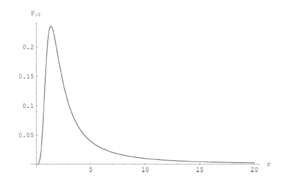
Figure 1: Electric field $F_{10}$ of the EBI- monopole as a function of r, for $M=0$, $r_{0}=1$, $m=1$, $n=3$ and $a=-0.9$ (see deatails in DCL )

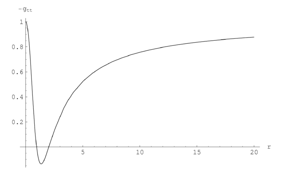
Figure 2: Coefficient $-gtt$ of the EBI - monopole in function of r, for$M=0$, $r_{0}=1$, $m=1$, $n=3$ and $a=-0.9$ (see details in DCL )

III.1 Equations for the electromagnetic fields

The equations that describe the dynamic of the electromagnetic fields of Born-Infeld in a curved spacetime are

$$\nabla_{a}\mathbb{F}^{ab}=\nabla_{a}\left[\frac{F^{ab}}{\mathbb{R}}+\frac{P}{b^{2}\mathbb{R}}\widetilde{F}^{ab}\right]=0\,\ \ \ \ \ \ \ \ \ \ \ \ \ \ \ \ \ \ \ \ \ \ \left(field\,equations\,\right)$$ (22)

$$\nabla_{a}\,\,\widetilde{F}^{ab}=0\,\ \ \ \ \ \ \ \ \ \ \ \ \ \ \ \ \ \ \ \ \ \ \ \ \ \ \ \ \ (\ Bianchi^{\prime}s\,\ identity)\ \ \ \ \ \ \ \ \ \ \ \ \ \ \ \ \ \ \ \ \ \ \ \ \ \ \ \ \ \ \ \ \ \$$ (23)

where the scalar and pseudoscalar invariants are

$$P\equiv-\frac{1}{4}F_{\alpha\beta}\widetilde{F}^{\alpha\beta}$$ (24)

$$S\equiv-\frac{1}{4}F_{\alpha\beta}F^{\alpha\beta}$$ (25)

$$\mathbb{R}\equiv\sqrt{1-\frac{2S}{b^{2}}-\left(\frac{P}{b^{2}}\right)^{2}}$$ (26)

The above equations can be solved explicitly in the tetrad from the line element(3)giving the follow result

$$F_{01}=A\left(r\right)$$ (27)

$$\mathbb{F}_{01}=f\ e^{-2G}$$ (28)

where $f$ is a constant. We can see from the above eqs. that

$$\mathbb{F}_{01}=\frac{F_{01}}{\sqrt{1-\left(\overline{F}_{01}\right)^{2}}}$$

where we obtain the following form for the electric field of the self-gravitating BI monopole

$$F_{01}=\frac{b}{\sqrt{\left(\frac{b}{f}e^{2G}\right)^{2}+1}}$$ (29)

Consequently, having into account the explicit expression for $f$

$$f=br_{0}^{2}\equiv Q\,\ \ \ \ \Rightarrow\,\ \ \ F_{01}=\frac{b}{\sqrt{\left(\frac{e^{G}}{r_{0}}\right)^{4}+1}}$$ (30)

The magnetic field is solved in an analog manner considering $F_{23}$ instead $F_{10}$ DCL . Where $r_{0}$ is a constant with units of longitude that in reference bi was associated to the radius of the electron. Finally the components of the energy-momentum tensor of BI takes its explicit form using the $F_{01}$ that we was found, namely

$$-T_{00}=T_{11}=\frac{b^{2}}{4\pi}\left(1-\sqrt{\left(\frac{r_{0}}{e^{G}}\right)^{4}+1}\right)$$ (31)

$$T_{22}=T_{33}=\frac{b^{2}}{4\pi}\left(1-\frac{1}{\sqrt{\left(\frac{r_{0}}{e^{G}}\right)^{4}+1}}\right)$$ (32)

IV General formalism

The starting point is the solution reviewed in the previous sections, that we rewrite as follows

$$ds^{2}=-A(r)dt^{2}+\frac{1}{B(r)}dr^{2}+C(r)(d\theta^{2}+\sin^{2}\theta d\phi^{2})$$ (33)

(e.g.: general static spherically symmetric space-time supposed with stationary regime) where the functions $A(r),B(r)$ and $C(r)$ have been determined according the general metric solution in Cirilo-Lombardo (2005) DCL :

$$A(r)=e^{2\Lambda}$$ (34)

$$B(r)=A(r)\left[\frac{dY_{i}(r)}{dr}\right]^{-2}$$ (35)

$$C(r)=r^{2}\left[K_{i}(r)\right]^{2m}$$ (36)

$$e^{2\Lambda}=1-\frac{2M}{Y_{i}}-\frac{2b^{2}r_{0}^{4}}{3(Y_{i}^{2}+\sqrt{Y_{i}^{4}+r_{0}^{4}})}-\frac{4}{3}b^{2}r_{0}^{2}~{}~{}_{2}F_{1}[1/4,1/2,5/4,-(Y/r_{0})^{4}]$$ (37)

where

$$r_{0}=\sqrt{\frac{e}{b}}$$ (38)

$e$ is the elementary charge and $b$ the fundamental field strength. ${}_{2}F_{1}[1/4,1/2,5/4,-(Y(r)/r_{0})^{4}]$ is the standard Hypergeometric Gauss Function and

$$Y_{i}(r)\equiv r\left[K_{i}(r)\right]^{m}\qquad i=1,2$$ (39)

Where we defined

$$K_{1}(r)\equiv 1-\left(\frac{r_{0}}{a|r|}\right)^{n}$$ (40)

$$K_{2}(r)\equiv\exp\left\{-\frac{r_{0}}{a|r|}n\right\}$$ (41)

being $K_{1}$ the ”kernel” of $Y_{1}$ proposed in Cirilo-Lombardo (2005) DCL and $K_{2}$ the new one proposed in this work for $Y_{2}$. Note that clearly $K_{1}$ and $K_{2}$ are subject to the properties of the electromagnetic field (due the boundary conditions, see Section II) by means of the BI energy-moment tensor, consequently modifying the metric (specifically coefficient A, B and C see33) through the gravitational EBI equations (they do not constitute a gauge due the boundary conditions as described in the Introduction). The advantage of $K_{2}(r)$over $K_{1}(r)$ is that the cusps of conical character in all the curves for n=1 near the origin are eliminated due the exponential (Yukawa) behaviour. Also the asymptotic behaviour is improved and controlled for all parameters of the model. Note that, as we saw earlier in $\mathcal{F}$, $K_{i}(r)$ is arbitrary but subject to the boundary conditions fixed by the physical scenario and the regularity conditions in the sense of DCL

V Dynamic equations of motion

In this section, we consider the simplest case of spherically symmetric stationary accretion. The stationarity assumes that the BH mass increases slowly, such that the distribution of the fluid on the relevant space-time scales has time to adjust itself to the changing BH metric. Following the procedure in Bahamonde and Jamil BJ15 we can write the 4-velocity under the restriction of spherical symmetry and stationary regime:

$$u^{\mu}=\frac{dx^{\mu}}{d\tau}=(u^{t},u^{r},0,0)$$ (42)

where $\tau$ is the proper time. This is a necessary step to compute the accretion rate. In this case all the variables are functions of $r$. Imposing the normalization condition, $u_{\mu}u^{\mu}=-1$ we have:

$$u^{t}\equiv\frac{dt}{d\tau}=\sqrt{\frac{u^{2}+B}{AB}}$$ (43)

$$u^{r}=\frac{dr}{dt}$$ (44)

From the energy-momentum conservation law:

$$0=T_{;\mu}^{\mu\nu}=\frac{1}{\sqrt{-g}}(\sqrt{-g})T_{,\mu}^{\mu\nu}+\Gamma_{\alpha\mu}^{\nu}T^{\alpha\mu}$$ (45)

we find:

$$(\rho+p)uC(r)\frac{A(r)}{B(r)}\sqrt{u^{2}+B(r)}=A_{1}$$ (46)

Projecting the 4-velocity onto the energy momentum conservation law we can obtain the energy flux continuity equation:

$$u^{\mu}\rho_{,\mu}+(\rho+p)u_{;\mu}^{\mu}=0$$ (47)

Pressure $p$ and density $\rho$ are related by an equation of state as:

$$p=p(\rho)$$ (48)

It is possible to obtain from (47):

$$\frac{\rho^{\prime}}{\rho+p}+\frac{u^{\prime}}{u}+\frac{A^{\prime}}{2A}+\frac{B^{\prime}}{2B}+\frac{C^{\prime}}{C}=0$$ (49)

where primes denotes derivatives respect to $r$. If we integrate this:

$$uC(r)\sqrt{\frac{A(r)}{B(r)}}e^{\int\frac{d\rho}{\rho+p(\rho)}}=-A_{0}$$ (50)

If we study accretion we need $u$; due to $A_{0}$ is an integration constant and, combining the fact that $T_{;\mu}^{\mu\nu}=0$

$$(\rho+p)\sqrt{u^{2}+B(r)}\sqrt{\frac{A(r)}{B(r)}}e^{-\int\frac{d\rho}{\rho+p(\rho)}}=A_{3}$$ (51)

where we defined $A_{3}=-A_{1}/A_{0}$. For spherical symmetry we take $\theta=\pi/2$ and we obtain from the metric determinant $\sqrt{-g}=C\sqrt{A/B}$. Finally, considering the equation of mass flux, $0=J_{;\mu}^{\mu}=\frac{1}{\sqrt{-g}}\frac{d}{dr}(J^{r}\sqrt{-g})$, we have:

$$\rho uC(r)\sqrt{\frac{A(r)}{B(r)}}=A_{2}$$ (52)

If we divide equations (46) and (52) we have:

$$\frac{(\rho+p)}{\rho}\sqrt{\frac{A(r)}{B(r)}}\sqrt{u^{2}+B(r)}=\frac{A_{1}}{A_{2}}\equiv A_{4}$$ (53)

$A_{1}$, $A_{2}$, $A_{3}$ and $A_{4}$ are integration constants. From the previous expression the accretion velocity is straighforward deduced. If we differentiate (52) and (53) following the procedure of BJ15 , we can obtain, the accretion rate:

$$\dot{M}_{acc}=4\pi A_{3}M_{eff}^{2}[p(r)+\rho(r)]$$ (54)

where the effective mass is:

$$M_{eff}\equiv 2M+Y_{i}(r)\left(\frac{2br_{0}^{4}}{3Y_{i}^{2}(r)+3\sqrt{Y_{i}^{4}(r)+r_{0}^{4}}}-\frac{4}{3}b^{2}r_{0}^{2}H(r)\right)$$ (55)

Due the absolute regular solutions (in the sense of (DCL, )), the density electromagnetically induced appearing in is:

$$\rho(r)=\frac{b^{4}r_{0}^{6}}{4\pi Y_{i}^{2}(r)}(\sqrt{1+Y_{i}^{4}(r)}-Y_{i}^{2}(r))$$ (56)

and the simplest choice for state equation for pressure, in order to compare with Bahamonde and Jamil’s paper BJ15 , is:

$$p(r)=(1+\omega)\rho(r)$$ (57)

Where $\omega$ is a correction(constant shift) to include different kinds of matter. Note that it is usually assumed in astrophysical scenarios that the matter flow accompanies the electromagnetic field lines. Finally, the expressions for electric $(F_{01})$and magnetic fields $(F_{23})$ are respectively:

$$E(r)=\frac{b}{\sqrt{1+Y_{i}^{4}(r)}}$$ (58)

$$B(r)=\frac{b}{Y_{i}^{2}(r)}$$ (59)

V.1 Particular cases for $m=1$, $n=\{1,3,5,7\}$ and $\omega=0$

In this section we had set for some selected values of $m$ and $n$ and computed the profiles of the metric coefficient, electric and magnetic fields, accretion velocity, accretion mass rate and density. In order to fix the main ideas, we had chosen the following values: $A_{4}=10$, $A_{2}=1$, $m=1$, $a=-0.9$   and normalized ones $M=1$, $e=1$, $b=3.8296591$ for all profiles.

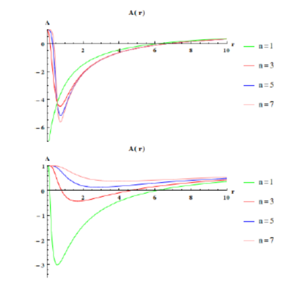
Figure 3: Metric coefficient $A(r)$ for $n=1,3,5,7$. (a) Top: Using $K_{1}$. (b) Bottom: Using $K_{2\text{.}}$

In Fig.3 we showed the profile of the metric coefficient for both kernels, $K_{1}$ at the top and $K_{2}$ at the bottom. The most clear effect imposed by $K_{2}$ is smoothing for $n={1,3,5,7}$ and regularized the profile of $A(r)$ for $n=1$.

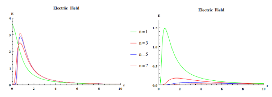
Figure 4: Electric field for $n=1,3,5,7$. (a) Left: Using $K_{1}$. (b) Right: Using $K_{2}$.

We can see the same behaviour in the electric and magnetic field, Fig.4 and Fig.5 comparing $K_{1}$ (left figures) with $K_{2}$ (right figures). In Fig.6 for the density is analogous.

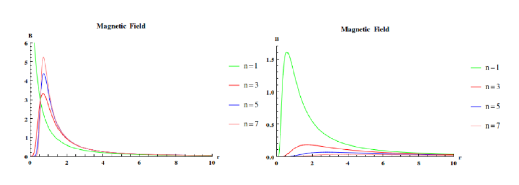
Figure 5: Magnetic field for $n=1,3,5,7$. (a) Left: Using $K_{1}$. (b) Right: Using $K_{2}$.

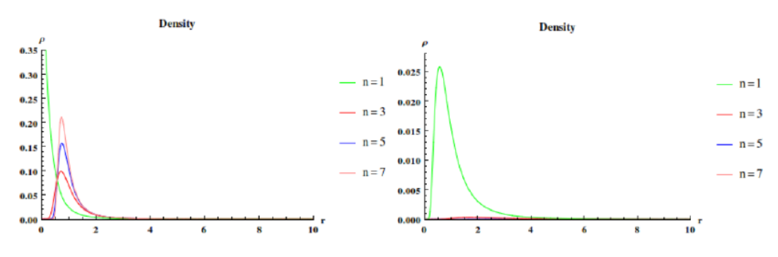
Figure 6: Density for $n=1,3,5,7$. (a) Left: Using $K_{1}$. (b) Right: Using $K_{2}$.

Respect to the accretion velocity, for $K_{1}$ the case $n=1$ is different to the case using $K_{2}$ where all profiles has the same shape with different intensities as shown in Fig.7

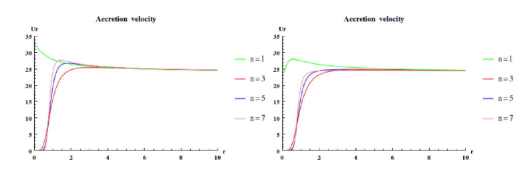
Figure 7: Accretion velocity for $n=1,3,5,7$. (a) Left: Using $K_{1}$. (b) Right: Using $K_{2}$.

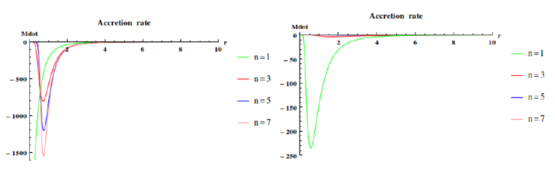
Figure 8: Accretion rate for $n=1,3,5,7$. (a) Left: Using $K_{1}$. (b) Right: Using $K_{2}$.

All the curves present qualitatively the same behaviour except the case $n=1$ using $K_{1}$, this case present accretion for the whole range of $r$, meanwhile the another velocities goes to zero when $r\rightarrow 0$. For $n\neq 1$ due to accretion velocity goes to zero could be interpreted as matter co-rotating near the central object in $r=0$. For $K_{2}$ disappears the divergence for $n=1$ as we expected. In Fig.8 the accretion mass rate is completely consistent with the fact that is related to accretion velocity, where the values changes in the velocity profiles according the changes in the curvature.

V.2 Introducing matter: Comparison for different values of $\omega$

We had set: $A_{4}=10$, $A_{2}=1$, $m=1$, $M=1$, $n=3$, $e=1$, $b=3.8296591$, $A_{0}=2+\omega$ and $a=-0.9$ for all profiles. In order to compare with BJ15 we choose different values of $\omega$ as we can see in Fig.9 and Fig.10.

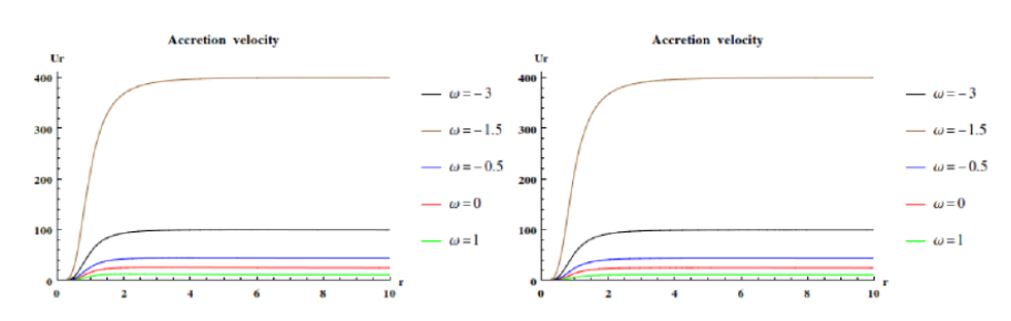
Figure 9: Accretion velocity for different values of $\omega$ Left: Using $K_{1}$. Right: Using $K_{2}$.

The cases where $\omega<0$ corresponds to Dark Matter. The values are chosen in order to compare with BJ15 . In particular, velocity profiles are far from Keplerian profiles as we can expect for galaxy models including Dark Matter qualitatively coherent with observational profiles. Also, as we can see in Fig.10 both kernels, $K_{1}$ and $K_{2}$ gives different accretion rates, however we have similar accretion velocities.

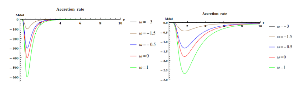
Figure 10: Accretion rate for different values of $\omega$ Left: Using $K_{1}$. Right: Using $K_{2}$.

V.3 BPS condition: the Reissner-Nordström limit

In this section we had set: $A_{4}=10$, $A_{2}=1$, $m=1$, $M=1$, $n=3$, $e=1$, $b=3.8296591$ $\omega=0$ and $a=-0.9$ for all profiles.

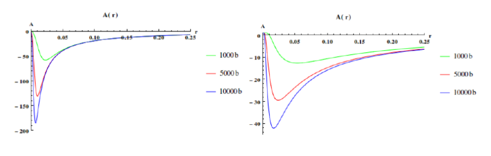
Figure 11: Metric coefficient $A\left(r\right)$ for $\ n=1,3,5,7.$ Left: Using $K_{1}.$ Right: Using $K_{2}$.

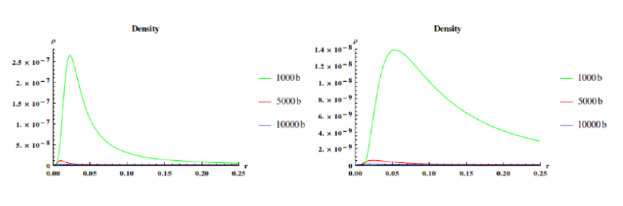
Figure 12: Density for $\ n=1,3,5,7.$ Left: Using $K_{1}.$ Right: Using $K_{2}$.

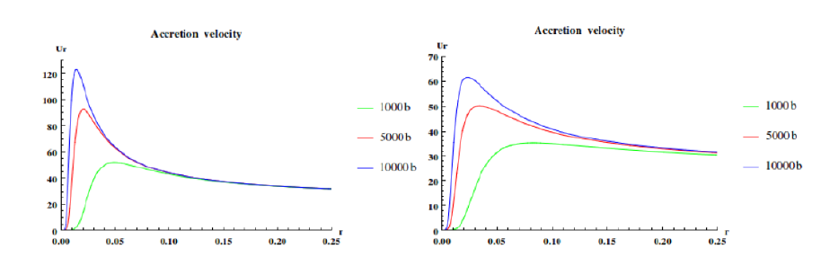
Figure 13: Accretion velocity for $\ n=1,3,5,7.$ Left: Using $K_{1}.$ Right: Using $K_{2}$.

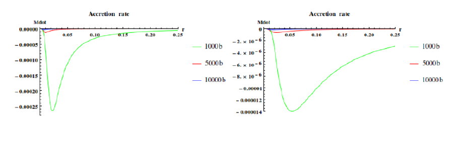
Figure 14: Accretion rate for $\ n=1,3,5,7.$ Left: Using $K_{1}.$ Right: Using $K_{2}$.

As it is known the action of EBI is the basis of the theories of great unification in particular theories containing supersymmetries as a fundamental ingredient. All these theories to be endowed with a high geometric content, such as theory of membranes, matrices and superstrings, which contain a non-linear non-commutative structure and therefore not local. In such theories the minimum energy condition or BPS corresponds to the linear or maxwellian limit, which in the case of Spherical Symmetric Solution (SSS) in theories of EBI are transformed into the solution of Reissner-Nordström (RN) limit. The importance from the astrophysical point of view that we propose here is that, when the condition of regularity is broken that is when one goes to the linear limit, the singularities appear generating the divergences that affect the mechanisms of stability and accretion.

In the case of unified theories as in the case of MacDowell-Mansouri 1979 manso and Cirilo-Lombardo 2017 diego17 , the limit value of the fields of the theory (which plays the role of the arbitrary parameter b in the standard EBI theory) is subject to the curvature and the dynamics of the same physical fields (states) that intervene both in the accretion and in the structure of space-time. This is completely in accordance with the conjecture in MacDowell-Mansouri 1979 and completely tested in Cirilo-Lombardo 2017.

VI Concluding remarks

In this work, we have been involved in the construction of gravastar models inspired in the full exact regular solutions of EBI nonlinear electrodynamics given in DCL and a new one of the Yukawa type. Although in this paper the back-reaction is not included, as is known, by means of a perturbative treatment, the back-reaction can be included in a simple manner with a minimum of modifications in both the Einstein equations and the accretion ones. Spherically symmetric solutions with a regular center (as our case) are stable before disturbancesbr , consequently the methods of treating the back-reaction are always favored in these scenarios Therefore, due to the full regularity in the gravastar models that we constructed, it is not necessary to regain the trouble with all type of spacetime singularities when accretion mechanisms are considered.

We use the proposed framework for the study of spherical accretion onto spherically symmetric compact objects given by Bahamonde and Jamil BJ15 . Despite having been indicated by those authors that the context of their proposal is the most general for spherically symmetric configurations, this proposal is only a rough approximation to the true problem of accretion of compact objects where time-dependent solutions are also necessary for a realistic description of the astrophysical process. We explored various features of our gravastar type solutions in the Bahamonde and Jamil framework considering no matter: e.g. only the selfgravitating nonlinear electromagmnetic configuration and with matter subject to the simplest state equation of type $p(r)=(1+\omega)\rho(r)$. This equation allows to see the behavior, in particular the stability of the solution before the accretion of normal matter and the exotic matter (dark matter) with respect to the values of the parameters chosen for both the particular solution of Cirilo-Lombardo (2005) DCL and the new solution of exponential type (Yukawa).

Concerning the accretion velocity profiles we can see that in the cases with exponential (Yukawa type ) solutions the shape of the curves are more smooth that in the case of the non exponential one DCL . Consequently we can expect that the inclusion in any galactic model of a regular EBI field can explain the several discrepancies between Modified Newtonian Dynamics (MOND) and pure dark matter proposals. If well in the actual research apparently when two modifications of the galaxy rotation curves from both MOND and the addition of Dark Matter change the curves in the desired way solving the troubles (by hand), this modification is only a static solution that works on simple systems. When applied to a more complex system the standard modifications does not solve the entire problem of the mass discrepancy and only manages to reduce the difference. The solution that Dark Matter provides is to add unobservable additional matter to the mass distribution. This idea of extra unseen mass is also supported by gravitational lensing experiments. There have been a number of propositions for the shape of the dark matter distribution, since this is unknown. These different proposals all lead to similar rotation curves with minor differences. Some rise quicker and decrease faster, like the Einasto-B profile, others rise slower but flatten off instead of decreasing, like the Burkert profile. Then, we remark here that in our case precisely the electromagnetic field through the density obtained from the same energy-momentum tensor, is able to show similar profiles to those considered empirically in galactic models of dark matter. Therefore the EBI electromagnetic fields in the context of regular spherically symmetric solutions must be considered together with the other proposals of both MOND and dark matter to solve all the discrepancies.

VII Acknowledgements

We gratefully acknowledge to the Departamento de Física (FCEyN, UBA) and Instituto de Física del Plasma (CONICET-UBA), DC is also grateful to the Consejo Nacional de Investigaciones Científicas y Técnicas and to the Bogoliubov Laboratory of Theoretical Physics, CV is also grateful to the Instituto de Ciencias (UNGS) for their institutional support.

References

- [1] M. Abou-Zeid. Actions for Curved Branes. arXiv High Energy Physics - Theory e-prints, January 2000.
- [2] M. A. Abramowicz, W. Kluzniak, and J.-P. Lasota. No observational proof of the black-hole event-horizon. A&A, 396:L31–L34, December 2002.
- [3] S. Bahamonde and M. Jamil. Accretion processes for general spherically symmetric compact objects. European Physical Journal C, 75:508, October 2015.
- [4] B. M. Barbashov and N. A. Chernikov. Scattering of two plane electromagnetic waves in the non-linear Born-Infeld electrodynamics. Communications in Mathematical Physics, 3:313–322, October 1966.
- [5] B. M. Barbashov and N. A. Chernikov. Solution and Quantization of a Nonlinear Two-dimensional Model for a Born-Infeld Type Field. Soviet Journal of Experimental and Theoretical Physics, 23:861, November 1966.
- [6] N. Bilic, G. B. Tupper, and R. D. Viollier. Born Infeld phantom gravastars. jcap, 2:013, February 2006.
- [7] M. Born. On the Quantum Theory of the Electromagnetic Field. Proceedings of the Royal Society of London Series A, 143:410–437, January 1934.
- [8] M. Born and L. Infeld. Foundations of the new field theory. Proc. Roy. Soc. Lond., A144(852):425–451, 1934.
- [9] K. A. Bronnikov, B. E. Meierovich, and E. R. Podolyak. Global monopole in general relativity. Soviet Journal of Experimental and Theoretical Physics, 95:392–403, September 2002.
- [10] B. M. N. Carter. Stable gravastars with generalized exteriors. Classical and Quantum Gravity, 22:4551–4562, November 2005.
- [11] C. Cattoen, T. Faber, and M. Visser. Gravastars must have anisotropic pressures. Classical and Quantum Gravity, 22:4189–4202, October 2005.
- [12] C. B. M. H. Chirenti and L. Rezzolla. How to tell a gravastar from a black hole. Classical and Quantum Gravity, 24:4191–4206, August 2007.
- [13] D. J. Cirilo Lombardo. New spherically symmetric monopole and regular solutions in Einstein-Born-Infeld theories. Journal of Mathematical Physics, 46(4):042501, April 2005.
- [14] D. J. Cirilo Lombardo. Non-Abelian Born-Infeld action, geometry and supersymmetry. Class. Quant. Grav., 22:4987–5004, 2005.
- [15] D. J. Cirilo-Lombardo. Non-Riemannian geometry, Born-Infeld models and trace free gravitational equations. Journal of High Energy Astrophysics, 16:1–14, December 2017.
- [16] J. Dai, R. G. Leigh, and J. Polchinski. New Connections Between String Theories. Modern Physics Letters A, 4:2073–2083, 1989.
- [17] A. DeBenedictis, D. Horvat, S. Ilijić, S. Kloster, and K. S. Viswanathan. Gravastar solutions with continuous pressures and equation of state. Classical and Quantum Gravity, 23:2303–2316, April 2006.
- [18] M. Demianski. Static electromagnetic geon. Foundations of Physics, 16:187–190, February 1986.
- [19] S. Deser and R. Puzalowski. J. Phys A: Math. and Gen., (13):2501, 1980.
- [20] M. J. Duff and C. J. Isham. Self-duality, helicity and coherent states in non-Abelian gauge theories. Nuclear Physics B, 162:271–284, January 1980.
- [21] D. O. Gómez. Accretion Power in Astrophysics, volume 1. AAABS, 2009.
- [22] T. Harko, Z. Kovács, and F. S. N. Lobo. Can accretion disk properties distinguish gravastars from black holes? Classical and Quantum Gravity, 26(21):215006, November 2009.
- [23] D. Horvat, S. Ilijić, and A. Marunović. Electrically charged gravastar configurations. Classical and Quantum Gravity, 26(2):025003, January 2009.
- [24] F. S. N. Lobo. Stable dark energy stars. Classical and Quantum Gravity, 23:1525–1541, March 2006.
- [25] F. S. N. Lobo and A. V. B. Arellano. Gravastars supported by nonlinear electrodynamics. Classical and Quantum Gravity, 24:1069–1088, March 2007.
- [26] S. W. MacDowell and F. Mansouri. Unified geometric theory of gravity and supergravity. Physical Review Letters, 38:739–742, April 1977.
- [27] P. O. Mazur and E. Mottola. Gravitational vacuum condensate stars. Proceedings of the National Academy of Science, 101:9545–9550, June 2004.
- [28] M. C. Miller. Implications of the gravitational wave event GW150914. General Relativity and Gravitation, 48:95, July 2016.
- [29] J. Plebanski. Lectures in Non-Linear electrodynamics. 1968.
- [30] A. A. Tseytlin. On non-abelian generalisation of the Born-Infeld action in string theory. Nuclear Physics B, 501:41–52, February 1997.
- [31] B. V. Turimov, B. J. Ahmedov, and A. A. Abdujabbarov. Electromagnetic Fields of Slowly Rotating Magnetized Gravastars. Modern Physics Letters A, 24:733–737, 2009.
- [32] N. Uchikata and S. Yoshida. Slowly rotating thin shell gravastars. Classical and Quantum Gravity, 33(2):025005, January 2016.
- [33] M. Visser and D. L. Wiltshire. Stable gravastars an alternative to black holes? Classical and Quantum Gravity, 21:1135–1151, February 2004.
- [34] E. Witten. Small instantons in string theory. Nuclear Physics B, 460:541–559, February 1996.